No-Signalling Assisted Zero-Error Capacity of Quantum Channels
and an
Information Theoretic Interpretation of the Lovász Number

Abstract

We study the one-shot zero-error classical capacity of a quantum channel assisted by quantum no-signalling correlations, and the reverse problem of exact simulation of a prescribed channel by a noiseless classical one. Quantum no-signalling correlations are viewed as two-input and two-output completely positive and trace preserving maps with linear constraints enforcing that the device cannot signal. Both problems lead to simple semidefinite programmes (SDPs) that depend only on the Kraus operator space of the channel. In particular, we show that the zero-error classical simulation cost is precisely the conditional min-entropy of the Choi-Jamiołkowski matrix of the given channel. The zero-error classical capacity is given by a similar-looking but different SDP; the asymptotic zero-error classical capacity is the regularization of this SDP, and in general we do not know of any simple form.

Interestingly however, for the class of classical-quantum channels, we show that the asymptotic capacity is given by a much simpler SDP, which coincides with a semidefinite generalization of the fractional packing number suggested earlier by Aram Harrow. This finally results in an operational interpretation of the celebrated Lovász $\vartheta$ function of a graph as the zero-error classical capacity of the graph assisted by quantum no-signalling correlations, the first information theoretic interpretation of the Lovász number.

I Introduction

We choose as the starting point of the present work the fundamental problem of channel simulation. Roughly speaking, this problem asks when a communication channel ${\cal N}$ from Alice (A) to Bob (B) can be used to simulate another channel ${\cal M}$, also from A to B? KretschmannWerner:tema This problem has many variants according to the resources available to A and B. In particular, the case when A and B can access unlimited amount of shared entanglement has been completely solved. Let $C_{E}({\cal N})$ denote the entanglement-assisted classical capacity of ${\cal N}$ BSST2003 . It was shown that, in the asymptotic setting, to optimally simulate ${\cal M}$, we need to apply ${\cal N}$ at rate $\frac{C_{E}({\cal M})}{C_{E}({\cal N})}$ BDHS+2009 ; QRST-simple . In other words, the entanglement-assisted classical capacity uniquely determines the properties of the channel in the simulation process. Furthermore, even with stronger resources such as no-signalling correlations or feedback, this rate cannot be improved – otherwise we would violate causality, see BDHS+2009 for a discussion.

Here we are interested in the zero-error setting Shannon1956 . It is well known that the zero-error communication problem is extremely difficult, already for classical channels. Indeed, the single-shot zero-error classical communication capability of a classical noisy channel equals the independence number of the (classical) confusability graph induced by the channel, and the latter problem is well-known to be NP-complete. The behaviour of quantum channels in zero-error communication is even more complex as striking effects such as super-activation are possible DS2008 ; Duan2009 ; CCH2009 ; CS2012 . The most general zero-error simulation problem remains wide open. To overcome this difficulty, many variants of this problem have been proposed. The most natural way is to introduce some additional resources and see how this changes the capacity. Indeed, extra resources such as classical feedback Shannon1956 , entanglement Duan2009 ; CLMW2010 ; DSW2010 , and even a small (constant) amount of forward communication CLMW2011 , have been introduced. It has been shown these extra resources can increase the capacity, and generally simplify the problem. In particular, it was shown that even for classical communication channel, shared entanglement can strictly increase the asymptotic zero-error classical capacity LMMO+2012 . However, determining the entanglement-assisted zero-error classical capacity remains an open problem even for classical channels. More powerful resources are actually required in order to simplify the problem. Cubitt et al. CLMW2011 introduced classical no-signalling correlations into the zero-error communication for classical channels, and showed that the well-known fractional packing number of the bipartite graph induced by the channel, gives precisely the zero-error classical capacity of the channel. Previously, it was known by Shannon that this fractional packing number corresponds to the zero-error classical capacity of the channel when assisted with a feedback link from the receiver to the sender and when the unassisted zero-error classical capacity is not vanishing Shannon1956 . For general background on graph theory see Berge , and for “fractional graph theory” the delightful book ScheinermanUllman .

Another major motivation for this work is to further explore the connection between quantum information theory and the so-called “non-commutative graph theory” suggested in DSW2010 . Such a connection has been well-known in classical information theory. In Shannon1956 , Shannon realized that the zero-error capacity of a classical noisy channel only depends on the confusability graph induced by the channel. He further pointed out that in the presence of classical feedback, the zero-error capacity is completely determined by the bipartite graph of possible input-output transitions associated with the channel. Thus it makes sense to talk about the zero-error capacity of a (bipartite) graph. The notion of non-commutative graph naturally occurs when we use quantum channels for zero-error communication. For any quantum channel, the non-commutative graph associated with the channel captures the zero-error communication properties, thus playing a similar role to confusability graph. Most notably, this notion also makes it possible to introduce a quantum Lovász $\vartheta$ function to upper bound the entanglement-assisted zero-error capacity that has properties quite similar to its classical analogue DSW2010 . Very recently, it was shown that the zero-error classical capacity of a quantum channel in the presence of quantum feedback only depends on the Kraus operator space of the channel DSW2013 . In other words, the Kraus operator space plays a role that is quite similar to the bipartite graph. Now it becomes clear that any classical channel induces a bipartite graph as well as a confusability graph, while a quantum channel induces a non-commutative bipartite graph and a non-commutative graph. The new insight is that we can simply regard a non-commutative (bipartite) graph as a high-level abstraction of all underlying quantum channels, and study its information-theoretic properties, not limited to zero-error setting. This leads us to a very general viewpoint: graphs as communication channels. For instance, we can define the entanglement-assisted classical capacity of a non-commutative bipartite graph as the minimum of the entanglement-assisted classical capacity of quantum channels that induce the given Kraus operator space. It was shown that this quantity enjoys a number of interesting properties including additivity under tensor product and an operational interpretation as a sort of entanglement-assisted conclusive capacity of the bipartite graph DSW2013 . It remains a great challenge to find tractable forms of various capacities for non-commutative (bipartite) graphs.

In this paper we consider a more general class of quantum no-signalling correlations described by two-input and two-output quantum channels with the no-signalling constraints. This kind of correlations naturally arises in the study of the relativistic causality of quantum operations BGNP2001 ; ESW2001 ; PHHH2006 ; see also the more recent OCB2012 . Distinguishability of these correlations from an information theoretic viewpoint has also been studied Chiribella2012 . We provide a number of new properties of these correlations, and establish several structural theorems of these correlations. Then we generalize the approach of CLMW2011 to study the zero-error classical capacity of a noisy quantum channel assisted by quantum no-signalling correlations, and the reverse problem of perfect simulation. We show that both problems can be completely solved in the one-shot scenario, revealing some nice structure:

1. The answers are given by semidefinite programmes (SDPs, cf. SDP );

2. At the same time they generalize the results of Cubitt et al. CLMW2011 ;

3. For the simulation, the question is really how to form a constant channel by a convex combination of the one we want to simulate and an arbitrary other quantum channel, and the number of bits needed is just $-\log p$, where $p$ is the probability weight of the target channel in the convex combination (throughout this paper, $\log$ denotes the binary logarithm);

4. For assisted communication, there is an analogous problem of convex-combing a certain channel from B to A which has some kind of orthogonality relation with the given channel from A to B, with another one to form a constant channel. If the target channel has weight $p$, then the number of bits sent is again $-\log p$.

Most interestingly, the solution to the communication problem only depends on the Kraus operator space of the channel, not directly on the channel itself. For the simulation problem, the solution is given by the conditional min-entropy KRS2009 ; Tomamichel-PhD of the channel’s Choi-Jamiołkowski matrix, and is actually additive, thus also gives the asymptotic cost of simulating the channel. If we are interested in simulating the cheapest channel contained in the Kraus operator space, we obtain an SDP in terms of the projection of the Choi-Jamiołkowski matrix. Both the capacity and the simulation SDPs are in general not known to be multiplicative under the tensor product of channels, thus we do not know the optimal asymptotic simulation cost.

We then focus on the asymptotic zero-error classical capacity and simulation cost assisted with quantum no-signalling correlations. This requires determining the asymptotic behaviour of a sequence of SDPs. In general the one-shot solution does not give the asymptotic result, since the corresponding SDP is not multiplicative with respect to the tensor product of channels. A simple formula for the asymptotic channel capacity remains unknown. However, for the special cases of classical-quantum (cq) channels, we find that the zero-error capacity is given by the solution of a rather simple SDP suggested earlier by Harrow as a natural generalization of the classical fractional packing number Harrow2010 , which we call semidefinite packing number. This result has two interesting corollaries. First, it implies that the zero-error classical capacity of cq-channels assisted by quantum no-signalling correlations is additive. Second, and more importantly, we show that for a classical graph $G$, the celebrated Lovász number $\vartheta(G)$ Lovasz1979 , is actually the minimum zero-error classical capacity of any cq-channel that has the given graph as its confusability graph. In other words, Lovász’ $\vartheta$ function is the zero-error classical capacity of a graph assisted by quantum no-signalling correlations. To the best of our knowledge, this is the first information theoretic operational interpretation of the Lovász number since its introduction in 1979. Previously, it was known that it is an upper bound on the entanglement-assisted zero-error classical capacity of a graph Beigi2010 ; DSW2010 . It remains unknown whether the use of quantum no-signalling correlations could be replaced by shared entanglement. The asymptotic simulation cost for Kraus operator spaces associated with cq-channels is rather simpler, and is actually given by the one-shot simulation cost.

Before we proceed to the technical details, it may be helpful to present an overview of our main results. Let ${\cal N}$ be a quantum channel from ${\cal L}(A^{\prime})$ to ${\cal L}(B)$, with a Kraus operator sum representation ${\cal N}(\rho)=\sum_{k}E_{k}\rho E_{k}^{\dagger},$ where $\sum_{k}E_{k}^{\dagger}E_{k}={\openone}_{A^{\prime}}$. Let $K=K({\cal N})=\operatorname{span}\{E_{k}\}$ denote the Kraus operator space of ${\cal N}$. The Choi-Jamiołkowski matrix of ${\cal N}$ is given by $J_{AB}=\sum_{ij}|i\rangle\!\langle j|_{A}\otimes{\cal N}(|i\rangle\!\langle j|_{A^{\prime}})=({\operatorname{id}}_{A}\otimes{\cal N})(|\Phi_{AA^{\prime}}\rangle\!\langle\Phi_{AA^{\prime}}|)$, where $A$ and $A^{\prime}$ are isomorphic Hilbert spaces, $\{|i\rangle\}$ ($\{|j\rangle\}$) is orthonormal basis over $A$ ($A^{\prime}$, resp.), and $|\Phi_{AA^{\prime}}\rangle=\sum_{k}|k_{A}\rangle|k_{A^{\prime}}\rangle$ is the unnormalized maximally entangled state over $A\otimes A^{\prime}$. Recall that $\operatorname{Tr}_{B}J_{AB}={\openone}_{A}$. Let $P_{AB}$ denote the projection onto the support of $J_{AB}$, which is the subspace $({\openone}_{A}\otimes K)|\Phi_{AA^{\prime}}\rangle$, sometimes called the Choi-Jamiołkowski support of $K$ (or of the channel).

It is worth noting that many results below can be defined on any matrix subspace $K$, not just those corresponding to a quantum channel ${\cal N}$. However, we have to make sure that $K$ is actually corresponding to some quantum channel ${\cal N}$. This puts an additional constraint on $K$. More precisely, suppose $K=\operatorname{span}\{E_{k}\}$ for some orthonormal basis $\{E_{k}\}$ such that $\operatorname{Tr}E_{j}^{\dagger}E_{k}=\delta_{jk}$. Then we should be able to find a quantum channel ${\cal N}^{\prime}=\sum_{j}F_{j}\cdot F_{j}^{\dagger}$ such that $F_{j}=\sum_{k}a_{jk}E_{k}$, for some invertible matrix $a=[a_{jk}]$ and $\sum_{j}F_{j}^{\dagger}F_{j}={\openone}_{A^{\prime}}$. This is equivalent to

$$\sum_{kl}r_{kl}E_{k}^{\dagger}E_{l}={\openone}_{A^{\prime}},\text{ where }r_{kl}=\sum_{j}a_{jk}^{*}a_{jl}.$$

If such a positive definite matrix $r=[r_{kl}]$ cannot be found, $K$ will not correspond to a quantum channel (nor any $K^{\otimes n}$ for $n\geq 1$). In this case one might still be able to find $K^{\prime}\subset K$ that is a Kraus operator space for some quantum channel ${\cal N}^{\prime}$. For instance, $K={\rm span}\{{\openone},|0\rangle\!\langle 1|\}$, and $K^{\prime}={\rm span}\{{\openone}\}$. (Note however that $K$ is the limit of the Kraus subspaces of genuine quantum channels, namely amplitude damping channels with damping parameter going to $0$; hence it might still be considered as admissible Kraus space of an infinitesimally amplitude damping channel.) We will, therefore, always assume that $K$ corresponds to some quantum channel ${\cal N}$ such that $K=K({\cal N})$. From now on, any such Kraus operator space $K$ will be alternatively called “non-commutative bipartite graph” – in fact, below we shall argue why it is a natural generalization of bipartite graphs.

Theorem 1

The one-shot zero-error classical capability, (quantified as the largest number of messages), of ${\cal N}$ assisted by quantum no-signalling correlations depends only on the non-commutative graph $K$, and is given by the integer part of the following SDP:

$$\begin{split}\Upsilon({\cal N})&=\Upsilon(K)\\ &=\max\operatorname{Tr}S_{A}\ \text{ s.t. }\ 0\leq E_{AB}\leq S_{A}\otimes{\openone}_{B},\operatorname{Tr}_{A}E_{AB}={\openone}_{B},\operatorname{Tr}P_{AB}(S_{A}\otimes{\openone}_{B}-E_{AB})=0,\end{split}$$

where $P_{AB}$ denotes the projection onto the the subspace $({\openone}\otimes K)|\Phi\rangle$.
Hence we are motivated to call $\Upsilon(K)$ the no-signalling assisted independence number of $K$.

The proof of this theorem will be given in Section III.1, where we also explore other properties of the above SDP. For another direction of investigation, looking at the specific channel ${\cal N}$ with Choi-Jamiołkowski matrix $J$ and trying to minimize the error probability for given number of messages, we refer the reader to the recent and highly relevant work of Leung and Matthews LeungMatthews , where exactly this is done in an environment with free no-signalling resources subject to other semidefinite constraints.

It is evident from this theorem that the one-shot zero-error classical capacity of ${\cal N}$ only depends on the Kraus operator space $K$. That is, any two quantum channels ${\cal N}$ and ${\cal M}$ will have the same capacity if they have the same Kraus operator space. For this reason, we usually use $\Upsilon(K)$ to denote $\Upsilon({\cal N})$. Furthermore, we can talk about the capacity of the Kraus operator space $K$ directly without referring to the underling quantum channel. Notice that a classical channel $N=(X,p(y|x),Y)$ naturally induces a bipartite graph $\Gamma(N)=(X,E,Y)$, where the input and output alphabets $X$ and $Y$ are the two sets of vertices, and $E\subset X\times Y$ is the set of edges such that $(x,y)\in E$ if and only if $p(y|x)>0$. We shall also use the notation $\Gamma(y|x)=1$ if $(x,y)\in E$, and $\Gamma(y|x)=0$ otherwise. In this case, we have

$$K(N)=K(\Gamma)=\operatorname{span}\{|y\rangle\!\langle x|\mathrel{\mathop{\mathchar 58\relax}}p(y|x)>0\},$$

and our notion $K({\cal N})$ generalizes this to arbitrary quantum channels.

Similarly, the simulation cost is given as follows.

Theorem 2

The one-shot zero-error classical simulation cost (quantified as the minimum number of messages) of a quantum channel ${\cal N}$ under quantum no-signalling assistance is given by $\lceil 2^{-H_{\min}(A|B)_{J}}\rceil$. Here, $J_{AB}=({\operatorname{id}}_{A}\otimes{\cal N})\Phi_{AA^{\prime}}$ is the Choi-Jamiołkowski matrix of ${\cal N}$, and $H_{\min}(A|B)_{J}$ is the conditional min-entropy defined as follows KRS2009 ; Tomamichel-PhD :

$$2^{-H_{\min}(A|B)_{J}}=\Sigma({\cal N})=\min\operatorname{Tr}T_{B},\ {\rm s.t.}\ J_{AB}\leq{\openone}_{A}\otimes T_{B}.$$

For example, the asymptotic zero-error classical simulation cost of the cq-channel $0\rightarrow\rho_{0}$ and $1\rightarrow\rho_{1}$, is given by $\log(1+D(\rho_{0},\rho_{1})),$ where $D(\rho_{0},\rho_{1})=\frac{1}{2}\|\rho_{0}-\rho_{1}\|_{1}$ is the trace distance between $\rho_{0}$ and $\rho_{1}$. This gives a new operational interpretation of the trace distance between $\rho_{0}$ and $\rho_{1}$ as the asymptotic exact simulation cost for the above cq-channel.

Since there might be more than one channel with Kraus operator space included in $K$, we are interested in the exact simulation cost of the “cheapest” among these channels. More precisely, the one-shot zero-error classical simulation cost of a Kraus operator space $K$ is defined as

$$\Sigma(K)=\min\{\Sigma({\cal N})\mathrel{\mathop{\mathchar 58\relax}}{\cal N}\text{ is quantum channel and }K({\cal N})<K\},$$

where $K({\cal N})<K$ means that $K({\cal N})$ is a subspace of $K$. Then it follows immediately from Theorem 2 that

Theorem 3

The one-shot zero-error classical simulation cost of a Kraus operator space $K$ under quantum no-signalling assistance is given by the integer ceiling of

$$\Sigma(K)=\min\operatorname{Tr}T_{B}\text{ s.t. }0\leq F_{AB}\leq{\openone}_{A}\otimes T_{B},\ \operatorname{Tr}_{B}F_{AB}={\openone}_{A},\ \operatorname{Tr}F_{AB}({\openone}_{AB}-P_{AB})=0,$$

where $P_{AB}$ is the projection onto the Choi-Jamiołkowski support of $K$.

We will prove these two theorems in Section III.2.

We introduce the asymptotic zero-error channel capacity of $K$ by considering the number of bits that can be communicated over $n$ copies of the channel ${\cal N}$, i.e. ${\cal N}^{\otimes n}$, having Kraus operator space $K^{\otimes n}$, per channel use as $n\rightarrow\infty$; we denote it as $C_{0,{\text{NS}}}(K)$. Likewise, the asymptotic number of bits needed per channel use to simulate ${\cal N}^{\otimes n}$ as $n\rightarrow\infty$, denoted $S_{0,{\text{NS}}}({\cal N})$, and the same minimized over all channels with Kraus operator space $K^{\otimes n}$ (not necessarily product channels!), which we denote $S_{0,{\text{NS}}}(K)$.

From these definitions, it is clear that they are given by the regularizations of the respective one-shot quantities:

$$S_{0,{\text{NS}}}({\cal N}) =-H_{\min}(A|B)_{J},$$ (1)

$$C_{0,{\text{NS}}}(K)=\sup_{n\geq 1}\frac{1}{n}\log\Upsilon\left(K^{\otimes n}\right),\quad S_{0,{\text{NS}}}(K) =\inf_{n\geq 1}\frac{1}{n}\log\Sigma\left(K^{\otimes n}\right),$$ (2)

the first one because $H_{\min}(A|B)$ is additive under tensor products.

So far, we are unable to determine closed formulas for the latter two in general. Interestingly, the special case of $K$ coming from a cq-channel can be solved completely. Note that if $K$ corresponds to a cq-channel ${\cal N}\mathrel{\mathop{\mathchar 58\relax}}i\longmapsto\rho_{i}$, with $P_{i}$ the projection over the support of $\rho_{i}$, then $K$ can be uniquely identified by a set of projections $\{P_{i}\}$ (up to a permutation over inputs). In this case,

$$K=\operatorname{span}\bigl{\{}|i\rangle\!\langle\psi|\mathrel{\mathop{\mathchar 58\relax}}|\psi\rangle\in\operatorname{supp}\,\rho_{i}\bigr{\}},\quad P=\sum_{i}|i\rangle\!\langle i|\otimes P_{i}.$$

Any such Kraus operator space will be called “non-commutative bipartite cq-graph” or simply “cq-graph”.

The case of assisted communication seems very complicated, and most interesting. We show that the zero-error classical capacity of cq-graphs is given by the solution of the following SDP:

$${\operatorname{\sf A}}(K)\mathrel{\mathop{\mathchar 58\relax}}=\max\sum_{i}s_{i}\ {\rm s.t.}~{}0\leq s_{i},\ \sum_{i}s_{i}P_{i}\leq{\openone}.$$ (3)

This number was suggested by Harrow as a natural generalization of the Shannon’s classical fractional packing number Harrow2010 , and we will refer to it as semidefinite (fractional) packing number associated with a set of projections $\{P_{i}\}$.

Our result can be summarized as

Theorem 4

The zero-error classical capacity of a cq-channel ${\cal N}\mathrel{\mathop{\mathchar 58\relax}}i\rightarrow\rho_{i}$ assisted by quantum no-signalling correlations is given by the logarithm of the semidefinite packing number ${\operatorname{\sf A}}(K)$, i.e.,

$$C_{0,{\rm NS}}(K)=\log{\operatorname{\sf A}}(K).$$

To be precise,

$$\frac{1}{\text{\rm poly}(n)}{\operatorname{\sf A}}(K)^{n}\leq\Upsilon\left(K^{\otimes n}\right)\leq{\operatorname{\sf A}}(K)^{n}.$$

The proof of this theorem is given in Section IV.2.

The asymptotic zero-error classical simulation cost for cq-graphs $K$ is relatively easy and straightforward. Indeed, we show that the one-shot zero-error classical simulation cost for cq-channels is multiplicative, i.e.

$$\Sigma(K_{1}\otimes K_{2})=\Sigma(K_{1})\,\Sigma(K_{2}),$$ (4)

for cq-graphs $K_{1}$ and $K_{2}$. The equality is proved by simply combining the sub-multiplicativity of the primal SDP and the super-multiplicativity of the dual problem, and then applying strong duality of SDPs. It readily follows that the asymptotic simulation cost for any Kraus operator $K$ corresponding to a cq-channel is given by the one-shot simulation cost, namely

$$S_{0,{\text{NS}}}(K)=\log\Sigma(K).$$ (5)

It is worth noting that the above equality is valid for many other cases. In particular, it holds when $K$ corresponds to a quantum channel that is an extreme point in the set of all quantum channels. It remains unknown whether this is true for more general $K$.

As an unexpected byproduct of our general analysis we obtain the following. To understand it, note that any cq-channel ${\cal N}\mathrel{\mathop{\mathchar 58\relax}}i\longmapsto\rho_{i}$ naturally induces a confusability graph $G$ on the vertices $i$, by letting $\{i,j\}\in E$ if and only if $\rho_{i}\not\perp\rho_{j}$, i.e. inputs $i$ and $j$ are confusable.

Theorem 5

For any classical graph $G$, the Lovász number $\vartheta(G)$ Lovasz1979 is the minimum zero-error classical capacity assisted by quantum no-signalling correlations of any cq-channel that induces $G$, i.e.

$$\log\vartheta(G)=\min\bigl{\{}C_{0,{\rm NS}}(K)\mathrel{\mathop{\mathchar 58\relax}}K^{\dagger}K<S_{G}\bigr{\}},$$

where the minimization is over cq-graphs $K$ and $S_{G}$ is the non-commutative graph corresponding to $G$ (see Eq. (46) in Section V).

In particular, equality holds for any cq-channel $i\rightarrow|\psi_{i}\rangle\!\langle\psi_{i}|$ such that $\{|\psi_{i}\rangle\}$ is an optimal orthogonal representation for $G$ in the sense of Lovász’ original definition Lovasz1979 .

The above result gives the first clear information theoretic interpretion of the Lovász $\vartheta$ function of a graph $G$, as the zero-error classical capacity of $G$ assisted by quantum no-signalling correlations, in the sense of taking the worst cq-channel with confusability graph $G$. Its proof will be given in Section V.

In Section VI, we provide results which completely characterize the feasibility (i.e., positivity) of zero-error communication with a non-commutative bipartite graph, or a quantum channel, assisted by no-signalling correlations. Finally, in Section VII, we conclude and propose several open problems for further study.

II Structure of quantum no-signalling correlations

II.1 Do quantum no-signalling correlations naturally occur in communication?

We will provide an intuitive explanation for how the quantum no-signalling correlations naturally arise from the information-theoretic viewpoint. Let ${\cal M}$ and ${\cal N}$ be two quantum channels both from A to B, and assume that A and B can access any quantum resources that cannot be used for communicating between them directly. An interesting question is to ask when ${\cal N}$ can exactly simulate ${\cal M}$? This class of resources clearly includes shared entanglement, and actually has some other more important members that are the central interest of this paper. We will derive some general constraints that all these resources should satisfy. Let us start with the one-shot case, that is, A and B can establish quantum channel ${\cal M}$ by using all “allowable resources” and one use of channel ${\cal N}$. We can abstractly represent the whole procedure as in Fig. 1; note that it falls within the formalism of “quantum combs” CD-AP , but as it is a rather special case we can understand it without explicitly invoking that theory.

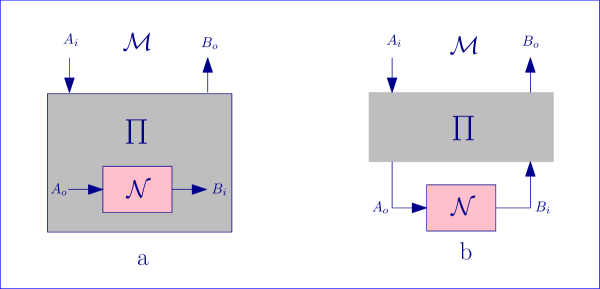
Figure 1: A general simulation network: a). We have abstractly represented the general simulation procedure for implementing a channel ${\cal M}$ using another channel ${\cal N}$ just once, and the correlations between A and B; b). This is just an equivalent way to redraw a), and we have highlighted all correlations between A an B, and their pre- and/or post- processing as $\Pi$.

Here is how this simulation works. First, A performs some pre-processing on the input quantum system $A_{i}$ together with all possible resources at her hand, and outputs quantum system $A_{o}$ as the input of channel ${\cal N}$. The channel ${\cal N}$ then outputs a quantum system $B_{i}$. B will do some post-processing on this system together with all possible resources he has, and finally generates an output $B_{o}$. If we remove ${\cal N}$, we are left with a network with two inputs $A_{i}$ and $B_{i}$, and two outputs $A_{o}$ and $B_{o}$. Clearly this represents all possible pre- and/or post-processing that A and B have done and all resources that are available to A and B. In the framework of quantum mechanics, this network can be formulated as a quantum channel $\Pi$ with two inputs and two outputs. Thus we can redraw the simulation procedure as Fig. 1.b. However, as ${\cal N}$ is the only communicating device from A to B, we must have that $\Pi$ cannot be used to communicate from A to B. Furthermore, the output $A_{o}$ represents the input of A to the channel ${\cal N}$, and thus can be uniquely determined by $A$, but not $B_{i}$, which is the output of ${\cal N}$. We will see this constraint is equivalent to B cannot communicate to A using $\Pi$. These constraints have led us to a fruitful class of resources that A and B could use in communication.

As before, we don’t attempt to solve the most general channel simulation problem. Instead, we will focus on two simpler but most interesting cases: i). ${\cal M}$ is a noiseless classical channel and ${\cal N}$ is the given noisy channel. The optimal solution to this problem will lead us to the notion of zero-error classical capacity of ${\cal N}$; ii). ${\cal N}$ is a noiseless classical channel and ${\cal M}$ is the given noisy channel. The optimal solution will lead us to the notion of zero-error classical simulation cost of ${\cal M}$. In the communication problem, we want to maximize the number of messages we can send exactly by the given channel; while in the simulation problem, we want to minimize the amount of the noiseless classical communication to simulate the given channel. In the rest of this section, we will study the mathematical structures of quantum no-signalling correlations in detail.

II.2 Mathematical definition of quantum no-signalling correlations

As discussed before, quantum no-signalling correlations are linear maps

$$\Pi\mathrel{\mathop{\mathchar 58\relax}}{\cal L}(A_{i})\otimes{\cal L}(B_{i})\rightarrow{\cal L}(A_{o})\otimes{\cal L}(B_{o})$$

with additional constraints. First, $\Pi$ is required to be completely positive (CP) and trace-preserving (TP). This makes $\Pi$ a physically realizable quantum operation. Furthermore, $\Pi$ is A to B no-signalling (A$\not\rightarrow$B). That is, A cannot send classical information to B by using $\Pi$. More precisely, for any density operators $\rho^{(0)}_{A_{i}},\rho^{(1)}_{A_{i}}\in{\cal L}(A_{i})$ and $\sigma_{B_{i}}\in{\cal L}(B_{i})$, we have

$$\operatorname{Tr}_{A_{o}}\Pi(\rho^{(0)}_{A_{i}}\otimes\sigma_{B_{i}})=\operatorname{Tr}_{A_{o}}\Pi(\rho^{(1)}_{A_{i}}\otimes\sigma_{B_{i}}).$$

Or equivalently,

$$\operatorname{Tr}_{A_{o}}\Pi(X_{A_{i}}\otimes Y_{B_{i}})=0\ \forall X,\ Y\text{ s.t. }\operatorname{Tr}X=0.$$

Likewise, $\Pi$ is required to be B to A no-signalling (B$\not\rightarrow$A). That is, B cannot send classical information to A by using $\Pi$. This constraint can be formulated as the following

$$\operatorname{Tr}_{B_{o}}\Pi(X_{A_{i}}\otimes Y_{B_{i}})=0\ \forall X,\ Y\text{ s.t. }\operatorname{Tr}Y=0.$$

Let the Choi-Jamiołkowski matrix of $\Pi$ be

$$\Omega_{A_{i}^{\prime}A_{o}B_{i}^{\prime}B_{o}}=({\operatorname{id}}_{A_{i}^{\prime}}\otimes{\operatorname{id}}_{B_{i}^{\prime}}\otimes\Pi)(\Phi_{A_{i}A_{i}^{\prime}}\otimes\Phi_{B_{i}B_{i}^{\prime}}),$$

where ${\operatorname{id}}_{A_{i}^{\prime}}$ is the identity operator over ${\cal L}(A_{i}^{\prime})$, $\Phi_{A_{i}A_{i}^{\prime}}=|\Phi_{A_{i}A_{i}^{\prime}}\rangle\!\langle\Phi_{A_{i}A_{i}^{\prime}}|$, and $|\Phi_{A_{i}A_{i}^{\prime}}\rangle=\sum_{k}|k_{A_{i}}\rangle|k_{A_{i}^{\prime}}\rangle$ the un-normalized maximally entangled state. We now show that all above constraints on $\Pi$ can be easily reformulated into the semidefinite programming constraints in terms of the Choi-Jamiołkowski matrix $\Omega$. For convenience, we often use unprimed letters such as $A_{i}$ and $B_{i}$ to denote the quantum systems inputting to quantum channels, and the primed letters $A_{i}^{\prime}$ and $B_{i}^{\prime}$ for the reference systems which are isomorphic to $A_{i}$ and $B_{i}$, respectively. The constraints on $\Pi$ can be equivalently formulated in terms of $\Omega$ as follows:

$$\Omega\geq 0, \quad(CP)$$

$$\operatorname{Tr}_{A_{o}B_{o}}\Omega={\openone}_{A_{i}^{\prime}B_{i}^{\prime}}, \quad(TP)$$

$$\operatorname{Tr}_{A_{o}A_{i}^{\prime}}\Omega X_{A_{i}^{\prime}}^{T}=0\ \forall\operatorname{Tr}X=0, \quad({\rm A}\not\rightarrow{\rm B})$$

$$\operatorname{Tr}_{B_{o}B_{i}^{\prime}}\Omega Y_{B_{i}^{\prime}}^{T}=0\ \forall\operatorname{Tr}Y=0, \quad({\rm B}\not\rightarrow{\rm A})$$

where $X$ and $Y$ are arbitrary Hermitian operators, so the transpose is not really necessary. The first two constraints guarantee that $\Omega$ corresponds to a CPTP map $\Pi$, while the latter two make sure that $\Omega$ cannot be used for communicating from A to B and B to A, respectively. Both constraints need only be verified on a Hermitian matrix basis of $A_{i}^{\prime}$, $B_{i}^{\prime}$, respectively.

The key to deriving the above constraints is the following useful fact:

$$X_{A}=\operatorname{Tr}_{A^{\prime}}\Phi_{AA^{\prime}}({\openone}_{A}\otimes{X^{T}_{A^{\prime}}})=\operatorname{Tr}_{A^{\prime}}\Phi_{AA^{\prime}}{X^{T}_{A^{\prime}}},$$

where $A^{\prime}$ is an isomorphic copy of $A$.

It is worth noting that the class of quantum no-signalling correlations is closed under convex combinations. That is, if $\Pi_{0}$ and $\Pi_{1}$ are quantum no-signalling correlations and $0\leq p\leq 1$, then $p\Pi_{0}+(1-p)\Pi_{1}$ are also no-signalling correlations. Furthermore, this class is also stable under the pre- or post-processing by A or B. That is, if $\Pi$ is a no-signalling correlation from ${\cal L}(A_{i}^{\prime}\otimes B_{i}^{\prime})$ to ${\cal L}(A_{o}\otimes B_{o})$. Then $\Pi^{\prime}=({\cal A}_{1}\otimes{\cal B}_{1})\Pi({\cal A}_{0}\otimes{\cal B}_{0})$ is also no-signalling, where ${\cal A}_{0},{\cal A}_{1},{\cal B}_{0},{\cal B}_{1}$ are CPTP maps on suitable Hilbert spaces.

It is instructive to compare the quantum no-signalling correlations and the classical no-signalling correlations. Recall that any classical no-signalling correlations can be described as a classical channel $Q=(X\times Y,Q(ab|xy),A\times B)$ with two classical inputs $x\in X$ and $y\in Y$, and two classical outputs $a\in A$ and $b\in B$, where

$$Q(ab|xy) \geq 0,\ \forall x\in X,y\in Y,a\in A,\ b\in B,$$ (6)

$$\sum_{ab}Q(ab|xy) =1,\ \forall x\in X,\ y\in Y,$$ (7)

$$\sum_{a}Q(ab|xy) =\sum_{a}Q(ab|x^{\prime}y),\ \forall x,x^{\prime}\in X,\ y\in Y,$$ (8)

$$\sum_{b}Q(ab|xy) =\sum_{b}Q(ab|xy^{\prime}),\ \forall x\in X,\ y,y^{\prime}\in Y.$$ (9)

Evidently, $Q$ can also be represented as a quantum channel in the following way

$$Q(\rho)=\sum_{a,b,x,y}Q(ab|xy)|ab\rangle\!\langle xy|\rho|xy\rangle\!\langle ab|.$$

One can easily verify the above constraints are exactly the same as treating $Q$ a quantum no-signalling correlation. From this viewpoint, quantum no-signalling correlations are natural generalizations of their classical correspondings.

Finally, we would like to mention another interesting fact. That is, any two-input and two-output quantum channel $\Pi$ can be reduced to a two-input and two-output classical channel $Q$ that has the same signalling property by simply doing pre- or post-processing, and all inputs and outputs of $Q$ are binary, i.e., if $\Pi$ is A to B (and/or B to A) signalling then $Q$ is also A to B (resp. B to A) signalling. Due to its significance, we formulate it as

Proposition 6

For any CPTP map $\Pi$ from ${\cal L}(A_{i}\otimes B_{i})$ to ${\cal L}(A_{o}\otimes B_{o})$ such that $\Pi$ is B to A (and/or A to B) signalling, one can obtain a classical channel $Q=(X\times Y,Q(ab|xy),A\times B)$ with all $|A|=|B|=|X|=|Y|=2$, by doing suitable local pre- and post-processing on $\Pi$, such that $Q$ is also B to A signalling (resp. A to B).

Proof.

Assume $\Pi$ is both way signalling (the case that it is one-way signalling is similar, and in fact simpler). Then we can find a pair of states $\rho^{(0)}_{A_{i}}$ and $\sigma^{(0)}_{B_{i}}$, such that the following two maps ${\cal A}\mathrel{\mathop{\mathchar 58\relax}}{\cal L}(A_{i})\rightarrow{\cal L}(B_{o})$ and ${\cal B}\mathrel{\mathop{\mathchar 58\relax}}{\cal L}(B_{i})\rightarrow{\cal L}(A_{o})$ are non-constant CPTP maps:

$${\cal A}(\rho_{A_{i}}) =\operatorname{Tr}_{A_{o}}\Pi(\rho_{A_{i}}\otimes\sigma^{(0)}_{B_{i}}),$$

$${\cal B}(\sigma_{B_{i}}) =\operatorname{Tr}_{B_{o}}\Pi(\rho^{(0)}_{A_{i}}\otimes\sigma_{B_{i}}).$$

I.e., we can find another two states $\rho^{(1)}_{A_{i}}$ and $\sigma^{(1)}_{B_{i}}$ such that

$${\cal A}(\rho^{(0)}_{A_{i}})\neq{\cal A}(\rho^{(1)}_{A_{i}}),~{}~{}{\cal B}(\sigma^{(0)}_{B_{i}})\neq{\cal B}(\sigma^{(1)}_{B_{i}}).$$

By Helstrom’s theorem, for any two different quantum states $\{\rho_{0},\rho_{1}\}$, we can find a projective measurement $\{P_{0},P_{1}\}$ to distinguish the given states with equal prior probably with an average success probability

$$p=\frac{1}{2}\operatorname{Tr}\rho_{0}P_{0}+\frac{1}{2}\operatorname{Tr}\rho_{1}P_{1}=\frac{1}{2}+\frac{1}{4}\|\rho_{0}-\rho_{1}\|_{1}>1/2.$$

As a direct consequence, the CPTP map

$${\cal M}(\rho)=(\operatorname{Tr}\rho P_{0})|0\rangle\!\langle 0|+(\operatorname{Tr}\rho P_{1})|1\rangle\!\langle 1|$$

will produce two different classical binary probability distributions ${\cal M}(\rho_{0})$ and ${\cal M}(\rho_{1})$. We will need this fact below.

Let $\bigl{(}P_{A_{o}}^{(0)},P_{A_{o}}^{(1)}\bigr{)}$ and $\bigl{(}Q_{B_{o}}^{(0)},Q_{B_{o}}^{(1)}\bigr{)}$ be the measurements to optimally distinguish $\bigl{\{}{\cal B}(\sigma^{(0)}_{B_{i}}),{\cal B}(\sigma^{(1)}_{B_{i}})\bigr{\}}$ and $\bigl{\{}{\cal A}(\rho^{(0)}_{A_{i}}),{\cal A}(\rho^{(1)}_{A_{i}})\bigr{\}}$, respectively. Then we can define four CPTP maps as follows:

$${\cal A}_{0}(\rho)=(\operatorname{Tr}|0\rangle\!\langle 0|\rho)\rho_{A_{i}}^{(0)}+(\operatorname{Tr}|1\rangle\!\langle 1|\rho)\rho_{A_{i}}^{(1)}, \quad{\cal A}_{1}(\rho)=(\operatorname{Tr}P_{A_{o}}^{(0)}\rho)|0\rangle\!\langle 0|+(\operatorname{Tr}P_{A_{o}}^{(1)}\rho)|1\rangle\!\langle 1|,$$

$${\cal B}_{0}(\sigma)=(\operatorname{Tr}|0\rangle\!\langle 0|\sigma)\sigma_{B_{i}}^{(0)}+(\operatorname{Tr}|1\rangle\!\langle 1|\sigma)\sigma_{B_{i}}^{(1)}, \quad{\cal B}_{1}(\sigma)=(\operatorname{Tr}Q_{B_{o}}^{(0)}\sigma)|0\rangle\!\langle 0|+(\operatorname{Tr}Q_{B_{o}}^{(1)}\sigma)|1\rangle\!\langle 1|.$$

Using these as pre- and post-processing on $\Pi$, we obtain the desired channel

$$Q=({\cal A}_{1}\otimes{\cal B}_{1})\circ\Pi\circ({\cal A}_{0}\otimes{\cal B}_{0}).$$

In $Q$, if B inputs $0$ or $1$, and A inputs $0$, then by the above construction, A must output two binary probability distributions that are different, hence can be used for signalling from B to A. Similarly, if A inputs $0$ or $1$, and B inputs $0$, then B must output another two different binary probability distributions that can be used for signalling from A to B.     $\sqcap$$\sqcup$

II.3 Structure theorems for quantum no-signalling correlations

We will establish several structure theorems regarding quantum no-signalling correlations. Note that $\Pi$ is a two-input and two-output quantum channel. So there are two natural ways to think of $\Pi$ according to the relation between the inputs and outputs. The first way is to partition $\Pi$ as $A_{i}A_{o}\mathrel{\mathop{\mathchar 58\relax}}B_{i}B_{o}$, so the output of $A_{i}$ and $B_{i}$ would be $A_{o}$ and $B_{o}$, respectively; this is perhaps the most standard way. The second way is to focus on the communication between $A$ and $B$ and partition $\Pi$ as $A_{i}B_{o}\mathrel{\mathop{\mathchar 58\relax}}B_{i}A_{o}$. In this case the output of $A_{i}$ and $B_{i}$ will be regarded as $B_{o}$ and $A_{o}$, respectively. This kind of partition is quite useful when we are interested in the communication between $A$ and $B$.

Let us start with the bipartition $A_{i}A_{o}\mathrel{\mathop{\mathchar 58\relax}}B_{i}B_{o}$ of $\Pi$. In this case, we can have a full characterization of no-signalling maps. (Bear in mind that we have assumed $\Pi$ to be a CPTP map in the following discussion).

Proposition 7

Let $\Pi\mathrel{\mathop{\mathchar 58\relax}}{\cal L}(A_{i})\otimes{\cal L}(B_{i})\rightarrow{\cal L}(A_{o})\otimes{\cal L}(B_{o})$ be a bipartite CPTP map with a decomposition $\Pi=\sum_{k}\lambda_{k}{\cal A}_{k}\otimes{\cal B}_{k}$ according to bipartition $A_{i}A_{o}\mathrel{\mathop{\mathchar 58\relax}}B_{i}B_{o}$, where ${\cal A}_{k}\mathrel{\mathop{\mathchar 58\relax}}{\cal L}(A_{i})\rightarrow{\cal L}(A_{o})$, ${\cal B}_{k}\mathrel{\mathop{\mathchar 58\relax}}{\cal L}(B_{i})\rightarrow{\cal L}(B_{o})$, and $\lambda_{k}$ are complex numbers. Then we have the following:

i) $\Pi$ is B to A no-signalling iff ${\cal B}_{k}$ can be chosen as CPTP for any $k$. In this case $\sum_{k}\lambda_{k}{\cal A}_{k}$ will be also CPTP.

ii) $\Pi$ is A to B no-signalling iff ${\cal A}_{k}$ can be chosen as CPTP for any $k$. In this case $\sum_{k}\lambda_{k}{\cal B}_{k}$ will be also CPTP.

iii) $\Pi$ is no-signalling between A and B iff both ${\cal A}_{k}$ and ${\cal B}_{k}$ can be chosen as CPTP maps, $\sum_{k}\lambda_{k}=1$, and $\lambda_{k}$ are real for all $k$.

The most interesting part is item iii). Intuitively, any no-signalling correlation $\Pi$ between A and B can be written as a real affine combination of product CPTP maps ${\cal A}_{k}\otimes{\cal B}_{k}$. The proofs are relatively straightforward and we simply leave them to interested readers as exercises.

Now we turn to the bipartition $A_{i}B_{o}\mathrel{\mathop{\mathchar 58\relax}}B_{i}A_{o}$ of $\Pi$. We don’t have a full characterization of no-signalling correlations in this setting. Nevertheless, a simple but extremely useful class of no-signalling correlations can be constructed using the following facts.

Proposition 8

Let $\Pi\mathrel{\mathop{\mathchar 58\relax}}{\cal L}(A_{i})\otimes{\cal L}(B_{i})\rightarrow{\cal L}(A_{o})\otimes{\cal L}(B_{o})$ be a bipartite CPTP map with a decomposition $\Pi=\sum_{k}\mu_{k}{\cal E}_{k}\otimes{\cal F}_{k}$ according to bipartition $A_{i}B_{o}\mathrel{\mathop{\mathchar 58\relax}}B_{i}A_{o}$, where ${\cal E}_{k}\mathrel{\mathop{\mathchar 58\relax}}{\cal L}(A_{i})\rightarrow{\cal L}(B_{o})$, ${\cal F}_{k}\mathrel{\mathop{\mathchar 58\relax}}{\cal L}(B_{i})\rightarrow{\cal L}(A_{o})$, and $\mu_{k}$ are complex numbers. Then we have the following:

i) If $\sum_{k}\mu_{k}{\cal E}_{k}$ is a constant map and ${\cal F}_{k}$ is TP for any $k$, then $\Pi$ is A to B no-signalling.

ii) If $\sum_{k}\mu_{k}{\cal F}_{k}$ is a constant map and ${\cal E}_{k}$ is TP for any $k$, then $\Pi$ is B to A no-signalling.

iii) If all ${\cal E}_{k}$ and ${\cal F}_{k}$ are TP and both $\sum_{k}\mu_{k}{\cal E}_{k}$ and $\sum_{k}\mu_{k}{\cal F}_{k}$ are constant maps, then $\Pi$ is no-signalling between A and B.

For example, we can choose $\Pi=\sum_{k}\mu_{k}{\cal E}_{k}\otimes{\cal F}_{k}$, where ${\cal E}_{k}$ and ${\cal F}_{k}$ are CPTP maps from ${\cal L}(A_{i})$ to ${\cal L}(B_{o})$ and ${\cal L}(B_{i})$ to ${\cal L}(A_{o})$, respectively, and $\{\mu_{k}\}$ is a probability distribution. If we further have that $\sum_{k}\mu_{k}{\cal E}_{k}$ and $\sum_{k}\mu_{k}{\cal F}_{k}$ are constant maps, then we obtain a no-signalling correlation $\Pi$. Clearly, for any such $\Pi$, neither of $A_{i}$ and $B_{i}$ can send classical information to $A_{o}$ or $B_{o}$. To emphasize this special feature, this class of no-signalling correlations are said to be totally no-signalling. We shall see later even this class of correlations could be very useful in assisting zero-error communication and simulation. In particular, we need the following technical result:

Lemma 9

Let ${\cal E}_{0}$ and ${\cal E}_{1}$ be two CPTP maps from ${\cal L}(A_{i})$ to ${\cal L}(B_{o})$, and let ${\cal F}_{0},{\cal F}_{1}$ be two CP maps from ${\cal L}(B_{i})$ to ${\cal L}(A_{o})$. Furthermore, assume there is unique $0\leq p\leq 1$ such that $p{\cal E}_{0}+(1-p){\cal E}_{1}$ is a constant channel. Then $\Pi=p{\cal E}_{0}\otimes{\cal F}_{0}+(1-p){\cal E}_{1}\otimes{\cal F}_{1}$ is a no-signalling correlation if and only if both ${\cal F}_{0}$ and ${\cal F}_{1}$ are CPTP maps, and $p{\cal F}_{0}+(1-p){\cal F}_{1}$ is a constant map.

Proof.

This can be proven by directly applying the definition of quantum no-signalling correlations. Two key points are: First, the uniqueness of $p$ such that $p{\cal E}_{0}+(1-p){\cal E}_{1}$ is constant; secondly, if ${\cal E}(X)=0$ for any traceless Hermitian operator $X$, ${\cal E}$ is a constant map.     $\sqcap$$\sqcup$

A third result about the structure of no-signalling correlations is the following ESW2001 (see also PHHH2006 for an alternate proof, and Chiribella2012 for more discussions):

Proposition 10

$\Pi$ is B$\not\rightarrow$A iff $\Pi={\cal G}\circ{\cal F}$ for two CPTP maps ${\cal F}\mathrel{\mathop{\mathchar 58\relax}}{\cal L}(A_{i})\rightarrow{\cal L}(A_{o}\otimes R)$ and ${\cal G}\mathrel{\mathop{\mathchar 58\relax}}{\cal L}(B_{i}\otimes R)\rightarrow{\cal L}(B_{o})$, where $R$ is an internal memory.     $\sqcap$$\sqcup$

This result is quite intuitive. It says that in the case that B cannot communicate to A, we can actually have the output of A before we input to B.

II.4 Composing no-signalling correlations with quantum channels

Suppose now we are given a no-signalling map $\Pi\mathrel{\mathop{\mathchar 58\relax}}{\cal L}(A_{i}\otimes B_{i})\rightarrow{\cal L}(A_{o}\otimes B_{o})$ and a CPTP map ${\cal N}\mathrel{\mathop{\mathchar 58\relax}}{\cal L}(A)\rightarrow{\cal L}(B)$. When $A=A_{o}$ and $B=B_{i}$, we can construct a new and unique map ${\cal M}\mathrel{\mathop{\mathchar 58\relax}}{\cal L}(A_{i})\rightarrow{\cal L}(B_{o})$ by feeding the output $A_{o}$ of $\Pi$ into ${\cal N}$, and use the output $B$ of ${\cal N}$ as the input $B_{i}$ to $\Pi$ (refer to Fig. 2). Next we will show how to derive more explicit forms of this map.

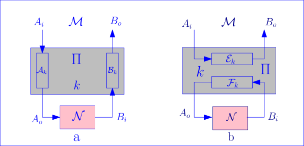
Figure 2: Two different partitions of the input-output registers of $\Pi$

Let us start by considering the partition according to $A_{i}A_{o}\mathrel{\mathop{\mathchar 58\relax}}B_{i}B_{o}$ to look at $\Pi$. If $\Pi$ is of product form ${\cal A}\otimes{\cal B}$ where ${\cal A}\mathrel{\mathop{\mathchar 58\relax}}{\cal L}(A_{i})\rightarrow{\cal L}(A_{o})$ and ${\cal B}\mathrel{\mathop{\mathchar 58\relax}}{\cal L}(B_{i})\rightarrow{\cal L}(B_{o})$, then clearly the composition must be given by ${\cal M}(X)={\cal B}\circ{\cal N}\circ{\cal A}(X)$. We can simply extend this construction to the superpositions of these product maps by linearity. I.e., for a general $\Pi=\sum_{k}{\cal A}_{k}\otimes{\cal B}_{k}$, we define the new map by composing ${\cal N}$ and $\Pi$ as the following

$${\cal M}^{A_{i}\rightarrow B_{o}}=\sum_{k}{\cal B}_{k}^{B_{i}\rightarrow B_{o}}\circ{\cal N}^{A_{o}\rightarrow B_{i}}\circ{\cal A}_{k}^{A_{i}\rightarrow A_{o}},$$ (10)

and this is clearly well-defined.

We can also formulate ${\cal M}$ in another useful way by considering the bipartition $A_{i}B_{o}\mathrel{\mathop{\mathchar 58\relax}}B_{i}A_{o}$. Suppose $\Pi$ is given in the form of $\sum_{k}{\cal E}_{k}\otimes{\cal F}_{k}$ where ${\cal E}_{k}\mathrel{\mathop{\mathchar 58\relax}}{\cal L}(A_{i})\rightarrow{\cal L}(B_{o})$, ${\cal F}_{k}\mathrel{\mathop{\mathchar 58\relax}}{\cal L}(B_{i})\rightarrow{\cal L}(A_{o})$.

Then to compose $\Pi$ and ${\cal N}$, the only thing we need to do is to compose ${\cal N}$ and ${\cal F}_{k}$ directly and take trace. That is, we have

$${\cal M}=\sum_{k}{\cal E}_{k}^{A_{i}\rightarrow B_{o}}\operatorname{Tr}({\cal F}_{k}\circ{\cal N}),$$ (11)

where the trace of super-operator ${\cal F}_{k}\circ{\cal N}$ on ${\cal L}(A_{o})$ is given by

$$\operatorname{Tr}{\cal F}_{k}\circ{\cal N}=\sum_{j}\operatorname{Tr}(C_{j}^{\dagger}({\cal F}_{k}\circ{\cal N})(C_{j}))$$

for any orthonormal basis $\{C_{j}\}$ on ${\cal L}(A_{o})$ in the sense of $\operatorname{Tr}(C_{j}^{\dagger}C_{l})=\delta_{jl}$. This is just the natural generalization of the trace function of the square matrices to super-operators. It is easy to verify that $\operatorname{Tr}({\cal F}\circ{\cal N})=\operatorname{Tr}({\cal N}\circ{\cal F})$ holds for any ${\cal F}$ and ${\cal N}$, and the trace is independent of the choice of the orthonormal basis $\{C_{j}\}$.

For instance, for any bipartite classical channel $Q=(X\times Y,Q(ab|xy),A\times B)$, and another classical channel $N=(A,N(y|a),Y)$, we can easily show that the map $M=(X,M(b|x),B)$ constructed by composing $Q$ and $N$ is given by

$$M(b|x)=\sum_{y,a}Q(ab|xy)N(y|a),$$

which coincides with the discussions in CLMW2011 .

Note that the above two constructions of the map ${\cal M}$ from $\Pi$ and ${\cal N}$ are quite general, and purely mathematical. Indeed, we can form a map ${\cal M}$ from any ${\cal N}$ and $\Pi$. An interesting and important question is to ask whether ${\cal M}$ is a CPTP map when both ${\cal N}$ and $\Pi$ are.

It turns out that whenever ${\cal N}$ and $\Pi$ are CP maps, ${\cal M}$ should also be CP. This fact is actually a simple corollary of the teleportation protocol. Indeed, we can easily see from the Fig. 3 that

$${\cal M}(X_{A_{i}})=\operatorname{Tr}_{BB_{i}^{\prime}}\{[(({\operatorname{id}}_{B_{o}B_{i}^{\prime}}\otimes{\cal N})\circ({\operatorname{id}}_{B_{i}^{\prime}}\otimes\Pi))(X_{A_{i}}\otimes\Phi_{B_{i}B_{i}^{\prime}})]({\openone}_{B_{o}}\otimes\Phi_{BB_{i}^{\prime}})\},$$ (12)

where $A=A_{o}$, and $B$, $B_{i}$, and $B_{i}^{\prime}$ are all isomorphic. The way to get the above equality is to first apply the teleportation protocol to the special case that $\Pi={\cal A}\otimes{\cal B}$, and then extend the result to the general case by linearity. The above expression not only provides a proof for the complete positivity of ${\cal M}$, but also the uniqueness of such ${\cal M}$.

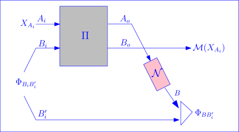
Figure 3: Composing ${\cal N}$ and $\Pi$ from the viewpoint of teleportation.

So we have obtained that for any two maps $\Pi\mathrel{\mathop{\mathchar 58\relax}}{\cal L}(A_{i}\otimes B_{i})\rightarrow{\cal L}(A_{o}\otimes B_{o})$ and ${\cal N}\mathrel{\mathop{\mathchar 58\relax}}{\cal L}(A_{o})\rightarrow{\cal L}(B_{i})$, we can uniquely construct a map ${\cal M}\mathrel{\mathop{\mathchar 58\relax}}{\cal L}(A_{i})\rightarrow{\cal L}(B_{o})$ by composing $\Pi$ and ${\cal N}$, and trace out $A_{o}$ and $B_{i}$. An explicit construction can be equivalently given by any of Eqs. (10), (11), and (12). Furthermore, if $\Pi$ and ${\cal N}$ are CP, so is ${\cal M}$.

To guarantee that ${\cal M}$ is TP, we have to put further constraints on $\Pi$, but not on ${\cal N}$ except that it is an arbitrary CPTP map. We will show that such constraints are precisely the same as the constraints that B to A no-signalling (B$\not\rightarrow$ A).

Proposition 11

Let $\Pi\mathrel{\mathop{\mathchar 58\relax}}{\cal L}(A_{i}\otimes B_{i})\rightarrow{\cal L}(A_{o}\otimes B_{o})$ and ${\cal N}\mathrel{\mathop{\mathchar 58\relax}}{\cal L}(A_{o})\rightarrow{\cal L}(B_{i})$ be two CPTP maps, and let ${\cal M}\mathrel{\mathop{\mathchar 58\relax}}{\cal L}(A_{i})\rightarrow{\cal L}(B_{o})$ be the unique CP constructed by composing $\Pi$ and ${\cal N}$. If $\Pi$ is CPTP and B to A no-signalling, then ${\cal M}$ is also CPTP for any CPTP map ${\cal N}$. Conversely, if ${\cal M}$ is CPTP for any ${\cal N}$, then $\Pi$ has to be B to A no-signalling.

Proof.

The sufficiency is just a direct corollary of item i) of Proposition 7 or Proposition 10. The later actually provides a physical realization of this map ${\cal M}$. This constraint is logically reasonable as B to A no-signalling simply means that the input of the channel ${\cal N}$ cannot depend on its output (otherwise we will have a closed loop, against the causality principle).

Now we will prove that the constraint of no-signalling from B to A is also necessary for ${\cal M}$ to be CPTP for any CPTP ${\cal N}$. Our strategy is to first prove this fact for two-input and two-output binary classical channel $Q$. Then we can apply Proposition 6 for the general case.

We can actually show that if $Q$ is signalling from B to A, and the composition of $Q$ and one-bit noiseless classical channel is not a legal classical channel anymore (the output for some input is not a legal probability distribution).

By contradiction, assume that the composition of $\Pi$ and any CPTP map ${\cal N}$ is always CPTP, but that $\Pi$ is B to A signalling. Applying Proposition 6, we can find a two-input and two-output binary classical channel $Q=(X\times Y,Q(ab|xy),A\times B)$ such that $Q$ is constructed from $\Pi$ by simply performing pre- and/or post-processing such that i) $Q=({\cal A}_{1}\otimes{\cal B}_{1})\circ\Pi\circ({\cal A}_{0}\otimes{\cal B}_{0})$; ii) $Q$ is also B to A signalling; iii) the composition of $Q$ and any classical channel $A$ to $Y$ is also a legal classical channel. We will show such $Q$ does not exist, hence complete the proof. Actually, ii) implies there are $x\in A,a\in A,y,y^{\prime}\in Y$, such that

$$\sum_{b=0}^{1}Q(ab|xy)\neq\sum_{b=0}^{1}Q(ab|xy^{\prime}).$$

w.o.l.g, we can assume $x=0$, $a=0$, $y=0$, and $y^{\prime}=1$. Then the above inequality can be rewritten explicitly as

$$Q(00|00)+Q(01|00)\neq Q(00|01)+Q(01|01).$$

On the other hand, the composition of $Q$ and a one-bit noiseless classical channel $N(y|a)=\delta_{ya}$ is given by

$$M(b|x)=\sum_{ya}Q(ab|xy)N(y|a)=\sum_{a=0}^{1}Q(ab|xa)=Q(0b|x0)+Q(1b|x1).$$

In particular, taking $x=0$ and applying the above inequality, we have

$$\begin{split}\sum_{b=0}^{1}M(b|0)&=Q(00|00)+Q(01|00)+Q(10|01)+Q(11|01)\\ &\neq Q(00|01)+Q(01|01)+Q(10|01)+Q(11|01)=1.\end{split}$$

This contradicts the fact that $M(b|x)$ is a classical channel.     $\sqcap$$\sqcup$

Thus, to guarantee that the composition ${\cal M}$ of a two-input and two-output channel $\Pi$ and any quantum channel from A to B is always a CPTP map, $\Pi$ is only required to be B to A no-signalling. The constraint of no-signalling from A to B is another natural requirement as we have assumed that A cannot communicate to B directly, and the given channel ${\cal N}$ is the only directed resource from A to B we can use. These considerations naturally lead us to quantum no-signalling correlations.

III Semidefinite programmes for zero-error communication
and simulation assisted by quantum no-signalling correlations

III.1 Zero-error assisted communication capacity

For any integer $M$, we denote by $M_{a}$ and $M_{b}$ classical registers with size $M$. We use ${\cal I}_{M}\mathrel{\mathop{\mathchar 58\relax}}M_{a}\rightarrow M_{b}$ to denote the noiseless classical channel that can send $M$ messages from $A$ to $B$, i.e. ${\cal I}_{M}(|m\rangle\!\langle m^{\prime}|_{M_{a}})=\delta_{mm^{\prime}}|m\rangle\!\langle m|_{M_{b}}$, or equivalenyly,

$${\cal I}_{M}(\rho)=\sum_{m=1}^{M}\bigl{(}\operatorname{Tr}\rho|m\rangle\!\langle m|_{M_{a}}\bigr{)}|m\rangle\!\langle m|_{M_{b}}.$$

If a channel ${\cal N}$ can simulate ${\cal I}_{M}$, we say that $M$ messages can be perfectly transmitted by one use of ${\cal N}$. The problem we are interested in is to determine the largest possible $M$, which will be called one-shot zero-error classical transmission capability of ${\cal N}$ assisted with no-signalling correlations. We restate here the result that we will prove in this subsection.

Theorem 1 The one-shot zero-error classical capability (quantified as the largest number of messages) of ${\cal N}$ assisted by quantum no-signalling correlations depends only on the non-commutative graph $K$, and is given by the integer part of the following SDP:

$$\begin{split}\Upsilon({\cal N})&=\Upsilon(K)\\ &=\max\operatorname{Tr}S_{A}\ \text{ s.t. }\ 0\leq E_{AB}\leq S_{A}\otimes{\openone}_{B},\operatorname{Tr}_{A}E_{AB}={\openone}_{B},\operatorname{Tr}P_{AB}(S_{A}\otimes{\openone}_{B}-E_{AB})=0,\end{split}$$

where $P_{AB}$ denotes the projection onto the the subspace $({\openone}\otimes K)|\Phi\rangle$.
Hence we are motivated to call $\Upsilon(K)$ the no-signalling assisted independence number of $K$.

Proof.

To make the indices of the Choi-Jamiołkowski matrices more readable, we reserve the unprimed letters such as $A_{i}$ and $B_{i}$ for the reference systems (thus as the indices of Choi-Jamiołkowski matrices), and use the primed versions $A_{i}^{\prime}$ and $B_{i}^{\prime}$ as the inputs to the quantum channels.

We will use a general no-signalling correlation $\Pi$ with Choi-Jamiołkowski matrix $\Omega$ and the channel ${\cal N}$, to exactly simulate a noiseless classical channel ${\cal I}_{M}$. Our goal is to determine the maximum integer $M$ when such simulation is possible. In this case both $A_{i}^{\prime}=M_{a}^{\prime}$ and $B_{o}=M_{b}$ are classical, and $A_{o}=A^{\prime}$, $B_{i}^{\prime}=B$. We will show that $\Omega$ can be chosen as the following form:

$$\Omega_{M_{a}M_{b}AB}=\frac{1}{M}D_{M_{a}M_{b}}\otimes E_{AB}+\frac{1}{M}({\openone}-D)_{M_{a}M_{b}}\otimes F_{AB},$$ (13)

where $D=\sum_{m}|mm\rangle\!\langle mm|$ is the Choi-Jamiołkowski matrix of the noiseless classical channel ${\cal I}_{M}$, and $E$ and $F$ are positive semidefinite operators. We will show that the no-signalling conditions are translated into

$$\operatorname{Tr}_{A}E_{AB}=\operatorname{Tr}_{A}F_{AB}={\openone}_{B}, \quad({\rm A}\not\rightarrow{\rm B}),$$ (14)

$$\frac{1}{M}E_{AB}+\left(1-\frac{1}{M}\right)F_{AB}=\sigma_{A}\otimes{\openone}_{B}, \quad({\rm B}\not\rightarrow{\rm A}),$$ (15)

with some state $\sigma$. In other words, both $E_{AB}$ and $F_{AB}$ are Choi-Jamiołkowski matrices of channels from ${\cal L}(B)$ to ${\cal L}(A)$ whose weighted sum is equal to a constant channel mapping quantum states in $B$ to a fixed state $\sigma_{A}$.

Let us first have a closer look at the the mathematical structure of $\Omega$. Rewrite $\Omega$ into the following form,

$$\Omega_{M_{a}M_{b}AB}=\frac{1}{M}D_{M_{a}M_{b}}\otimes E_{AB}+\left(1-\frac{1}{M}\right)\tilde{D}_{M_{a}M_{b}}\otimes F_{AB},$$

where $\tilde{D}_{M_{a}M_{b}}=\frac{1}{M-1}({\openone}-D)_{M_{a}M_{b}}$ is the Choi-Jamiołkowski matrix of the classical channel $\widetilde{{\cal I}}_{M}$ that sends each $m$ into a uniform distribution of $m^{\prime}\neq m$. In other words, the no-signalling correlation $\Pi$ should have the following form:

$$\Pi=\frac{1}{M}{\cal I}_{M}\otimes{\cal E}+\left(1-\frac{1}{M}\right)\widetilde{{\cal I}}_{M}\otimes{\cal F},$$ (16)

and ${\cal E}$ and ${\cal F}$ are CP maps from $B$ to $A$ corresponding to Choi-Jamiołkowski matrices $E_{AB}$ and $F_{AB}$, respectively.

Now we can directly apply Lemma 9 to $\Pi$ in Eq. (16) to obtain the no-signalling constraints in Eqs. (14) and (15). First, the constraints for ${\rm A}\not\rightarrow{\rm B}$ are automatically satisfied due to the special forms of ${\cal I}_{M}$ and $\widetilde{{\cal I}}_{M}$, and $p=1/M$ is the unique number such that $\frac{1}{M}{\cal I}_{M}+\left(1-\frac{1}{M}\right)\widetilde{{\cal I}}_{M}$ is constant. The no-signalling constraint ${\rm B}\not\rightarrow{\rm A}$ is equivalent to that ${\cal E}$ and ${\cal F}$ are CPTP maps, and $\frac{1}{M}{\cal E}+\left(1-\frac{1}{M}\right){\cal F}$ is some constant channel.

When composing ${\cal N}$ with $\Pi$ in Eq. (16), we have the following channel

$${\cal M}=\frac{1}{M}{\cal I}_{M}\operatorname{Tr}({\cal N}\circ{\cal E})+\left(1-\frac{1}{M}\right)\widetilde{{\cal I}}_{M}\operatorname{Tr}({\cal N}\circ{\cal F}).$$

The zero-error constraint requires ${\cal M}={\cal I}_{M}$, which is equivalent to $\operatorname{Tr}({\cal N}\circ{\cal F})=0$, or

$$\operatorname{Tr}F_{AB}J_{AB}=0,$$

where $J_{AB}=({\cal N}^{\dagger}\otimes{\operatorname{id}}_{B})(\Phi_{B^{\prime}B})$ is the Choi-Jamiołkowski matrix of ${\cal N}$ (strictly speaking, this is the complex conjugate of the Choi-Jamiołkowski matrix of ${\cal N}$, but this does not make any difference to the problem we are studying).

Since $E_{AB}$ and $F_{AB}$ depend on each other, we can eliminate one of them. For instance, we only keep $E_{AB}$. Then the existence of $F_{AB}$ will be equivalent to

$$\operatorname{Tr}_{A}E_{AB}={\openone}_{B},0\leq E_{AB}\leq M\sigma_{A}\otimes{\openone}_{B},\operatorname{Tr}P_{AB}(M\sigma_{A}\otimes{\openone}_{B}-E_{AB})=0.$$

By absorbing $M$ into $\sigma_{A}$ and introducing $S_{A}=M\sigma_{A}$, we get $M$ as the integer part of

$$\max\operatorname{Tr}S_{A}\text{ s.t. }0\leq E_{AB}\leq S_{A}\otimes{\openone}_{B},\operatorname{Tr}_{A}E_{AB}={\openone}_{B},\ \operatorname{Tr}P_{AB}(S_{A}\otimes{\openone}_{B}-E_{AB})=0,$$ (17)

which ends the proof.     $\sqcap$$\sqcup$

Now we provide a detailed derivation of the form (13) of the no-signalling correlation. Assume the channel is ${\cal N}\mathrel{\mathop{\mathchar 58\relax}}{\cal L}(A)\rightarrow{\cal L}(B^{\prime\prime})$, and the no-signalling correlation we will use is $\Pi\mathrel{\mathop{\mathchar 58\relax}}{\cal L}(M_{a}^{\prime}\otimes B^{\prime})\rightarrow{\cal L}(A\otimes M_{b})$. Suppose we can send $M$ messages exactly by one use of the channel ${\cal N}$ when assisted by $\Pi$. Then we should have (refer to Fig. 3 and note $A_{i}=M_{a}^{\prime}$, $A_{o}=A$, $B=B^{\prime\prime}$, $B_{i}^{\prime}=B$, and $B_{o}=M_{b}$)

$$\operatorname{Tr}_{BB^{\prime\prime}}[\Phi_{BB^{\prime\prime}}(({\cal N}\otimes{\operatorname{id}}_{M_{b}B})\circ(\Pi\otimes{\operatorname{id}}_{B}))(|m\rangle\!\langle m|_{M_{a}^{\prime}}\otimes\Phi_{B^{\prime}B})]=|m\rangle\!\langle m|_{M_{b}}\ \forall m\in\{1,\ldots,M\}.$$ (18)

The Choi-Jamiołkowski matrix of $\Pi$, say $\Omega_{M_{a}M_{b}AB}$, should satisfy the following constraints

$$\Omega_{M_{a}M_{b}AB}\geq 0,\ \operatorname{Tr}_{AM_{b}}\Omega_{M_{a}M_{b}AB}={\openone}_{M_{a}B}.$$

Furthermore, noticing that

$$|m\rangle\!\langle m|_{M_{a}^{\prime}}=\operatorname{Tr}_{M_{a}}(\Phi_{M_{a}^{\prime}M_{a}}({\openone}_{M_{a}^{\prime}}\otimes|m\rangle\!\langle m|_{M_{a}}^{T}))\ \text{and}\ |m\rangle\!\langle m|=|m\rangle\!\langle m|^{T},$$

we have

$$(\Pi\otimes{\operatorname{id}}_{B})(|m\rangle\!\langle m|_{M_{a}^{\prime}}\otimes\Phi_{B^{\prime}B})=\operatorname{Tr}_{M_{a}}(\Omega_{M_{a}M_{b}AB}\cdot(|m\rangle\!\langle m|_{M_{a}}\otimes{\openone}_{M_{b}AB})).$$

Thus the left hand side (l.h.s) of Eq. (18) gives, for all $m\in\{1,\ldots,M\}$,

$$\operatorname{Tr}_{BB^{\prime\prime}M_{a}}[(({\cal N}\otimes{\operatorname{id}}_{M_{a}M_{b}B})\Omega_{M_{a}M_{b}AB})(\Phi_{BB^{\prime\prime}}\otimes|m\rangle\!\langle m|_{M_{a}}\otimes{\openone}_{M_{b}})]=|m\rangle\!\langle m|_{M_{b}}.$$

In other words, for any $m\neq m^{\prime}$, we have

$$\operatorname{Tr}\bigl{(}(({\cal N}\otimes{\operatorname{id}}_{M_{a}M_{b}B})\Omega_{M_{a}M_{b}AB})(\Phi_{BB^{\prime\prime}}\otimes|m\rangle\!\langle m|_{M_{a}}\otimes|m^{\prime}\rangle\!\langle m^{\prime}|_{M_{b}})\bigr{)}=0.$$

The next crucial step is to simplify the form of $\Omega$. We will study all the possible forms of $\Omega$ satisfying the above equation. (Any such operator is said to be feasible). Since both $M_{a}$ and $M_{b}$ are classical registers, we can perform the dephasing operation on them and assume $\Omega$ has the following form

$$\Omega=\sum_{m=1}^{M}\sum_{m^{\prime}=1}^{M}|mm^{\prime}\rangle\!\langle mm^{\prime}|_{M_{a}M_{b}}\otimes\Omega_{AB}^{(mm^{\prime})},$$

where $\Omega_{AB}^{(mm^{\prime})}$ might not be identical for different pairs $(m,m^{\prime})$.

To further simplify the form of $\Omega$, we next exploit the permutation invariance of ${\cal I}_{M}$. More precisely, for any $M\times M$ permutation $\tau\in S_{M}$, if $\Omega_{M_{a}M_{b}AB}$ is feasible, then

$$\Omega_{M_{a}M_{b}AB}^{\prime}=(\tau_{M_{a}}\otimes\tau_{M_{b}}\otimes{\openone}_{AB})\Omega_{M_{a}M_{b}AB}(\tau_{M_{a}}\otimes\tau_{M_{b}}\otimes{\openone}_{AB})^{\dagger}$$

is also feasible. Furthermore, if $\Omega^{\prime}$ and $\Omega^{\prime\prime}$ are feasible, so is any convex combination $\lambda\Omega^{\prime}+(1-\lambda)\Omega^{\prime\prime}$ for $0\leq\lambda\leq 1$. With these two observations, from any feasible $\Omega$ that has been dephased, we can always construct a new feasible $\tilde{\Omega}$ by performing the following twirling operation

$$\tilde{\Omega}_{M_{a}M_{b}AB}=\frac{1}{M!}\sum_{\tau\in S_{M}}(\tau_{M_{a}}\otimes\tau_{M_{b}}\otimes{\openone}_{AB})\Omega_{M_{a}M_{b}AB}(\tau_{M_{a}}\otimes\tau_{M_{b}}\otimes{\openone}_{AB})^{\dagger}.$$

By applying Schur’s Lemma to the symmetry group $\{\tau_{M_{a}}\otimes\tau_{M_{b}}\mathrel{\mathop{\mathchar 58\relax}}\tau\in S_{M}\}$, we can see that $\tilde{\Omega}$ can be chosen as the following form

$$\tilde{\Omega}_{M_{a}M_{b}AB}=\sum_{m}|mm\rangle\!\langle mm|_{M_{a}M_{b}}\otimes\Omega_{AB}^{=}+\sum_{m\neq m^{\prime}}|mm^{\prime}\rangle\!\langle mm^{\prime}|\otimes\Omega_{AB}^{\neq},$$

which has exactly the same form as Eq. (13).

The SDP characterization of Theorem 1,

$$\begin{split}\Upsilon(K)&=\max\operatorname{Tr}S_{A}\ \text{ s.t. }\ 0\leq E_{AB}\leq S_{A}\otimes{\openone}_{B},\\ &\phantom{=\max\operatorname{Tr}S_{A}\text{ s.t. }}\operatorname{Tr}_{A}E_{AB}={\openone}_{B},\\ &\phantom{=\max\operatorname{Tr}S_{A}\text{ s.t. }}\operatorname{Tr}P_{AB}(S_{A}\otimes{\openone}_{B}-E_{AB})=0,\end{split}$$ (19)

has a dual. It is given by

$$\begin{split}\Upsilon(K)&=\min\operatorname{Tr}T_{B}\ \text{ s.t. }\ z\geq 0,\ W_{AB}\geq 0,\\ &\phantom{=\min\operatorname{Tr}T_{B}\text{ s.t. }}zP_{AB}-W_{AB}\leq{\openone}_{A}\otimes T_{B},\\ &\phantom{=\min\operatorname{Tr}T_{B}\text{ s.t. }}\operatorname{Tr}_{B}(zP-W)_{AB}={\openone}_{A}\\ &=\min\operatorname{Tr}T_{B}\ \text{ s.t. }\ F_{AB}\leq{\openone}_{A}\otimes T_{B},\\ &\phantom{=\min\operatorname{Tr}T_{B}\text{ s.t. }}\operatorname{Tr}_{B}F_{AB}={\openone}_{A},\\ &\phantom{=\min\operatorname{Tr}T_{B}\text{ s.t. }}({\openone}-P)_{AB}F_{AB}({\openone}-P)_{AB}\leq 0,\end{split}$$ (20)

which can be derived by the usual means; by strong duality, which applies here, the values of both the primal and the dual SDP coincide.

For an easy example of the evaluation of these SDPs, $\Upsilon(\Delta_{\ell})=\ell$ for the cq-graph $\Delta_{\ell}$ of the noiseless classical channel ${\cal I}_{\ell}$ of $\ell$ symbols. The Kraus operator space of the noiseless $\ell$-level quantum channel ${\operatorname{id}}_{\ell}$ is ${{\mathbb{C}}}{\openone}$, and has $\Upsilon({{\mathbb{C}}}{\openone})=\ell^{2}$.

Remark  By inspection of the primal SDP, for any $K_{1}$ and $K_{2}$, $\Upsilon(K_{1}\otimes K_{2})\geq\Upsilon(K_{1})\Upsilon(K_{2})$, because the tensor product of feasible solutions of the SDP (19) is feasible for $K_{1}\otimes K_{2}$. In particular, $\Upsilon(K\otimes\Delta_{\ell})\geq\ell\,\Upsilon(K)$. We do not know whether equality holds here (sometimes it does); the most natural way for proving this would be to use the dual SDP (20), but to use it to show “$\leq$” by tensoring together dual feasible solutions would require that $T\geq 0$.

Leaving this aside, this last observation is why $\Upsilon(K)$ is rightfully called the no-signalling assisted independence number, and not its integer part. Indeed, the number of messages we can send via $K\otimes\Delta_{\ell}$ is $\lfloor\Upsilon(K\otimes\Delta_{\ell})\rfloor>\ell\lfloor\Upsilon(K)\rfloor$, for non-integer $\Upsilon(K)$ and sufficiently large $\ell$.     $\sqcap$$\sqcup$

III.2 Zero-error assisted simulation cost

For convenience we restate here the two theorems already announced in the introduction.

Theorem 2 The one-shot zero-error classical simulation cost (quantified as the minimum number of messages) of a quantum channel ${\cal N}$ under quantum no-signalling assistance is given by $\lceil 2^{-H_{\min}(A|B)_{J}}\rceil$. Here, Here, $J_{AB}=({\operatorname{id}}_{A}\otimes{\cal N})\Phi_{AA^{\prime}}$ is the Choi-Jamiołkowski matrix of ${\cal N}$, and $H_{\min}(A|B)_{J}$ is the conditional min-entropy defined as follows KRS2009 ; Tomamichel-PhD :

$$2^{-H_{\min}(A|B)_{J}}=\Sigma({\cal N})=\min\operatorname{Tr}T_{B},\ {\rm s.t.}\ J_{AB}\leq{\openone}_{A}\otimes T_{B}.$$

Theorem 3 The one-shot zero-error classical simulation cost of a Kraus operator space $K$ under quantum no-signalling assistance is given by the integer ceiling of

$$\Sigma(K)=\min\operatorname{Tr}T_{B}\text{ s.t. }0\leq F_{AB}\leq{\openone}_{A}\otimes T_{B},\ \operatorname{Tr}_{B}F_{AB}={\openone}_{A},\ \operatorname{Tr}F_{AB}({\openone}_{AB}-P_{AB})=0,$$

where $P_{AB}$ denotes the projection onto the subspace $({\openone}\otimes K)|\Phi\rangle$.

Proof.

In this case we have $A_{o}=M_{a}$ and $B_{i}=M_{b}$ are classical, $A_{i}=A$, $B_{o}=B$. We will show that w.l.o.g.

$$\Omega_{ABM_{a}M_{b}}=\frac{1}{M}E_{AB}\otimes D_{M_{a}M_{b}}+\left(1-\frac{1}{M}\right)F_{AB}\otimes\tilde{D}_{M_{a}M_{b}},$$ (21)

with positive semidefinite $E_{AB}$ and $F_{AB}$. Then according to Lemma 9, the no-signalling conditions are equivalent to

$$\operatorname{Tr}_{B}E_{AB}=\operatorname{Tr}_{B}F_{AB} ={\openone}_{A},$$

$$\frac{1}{M}E_{AB}+\left(1-\frac{1}{M}\right)F_{AB} ={\openone}_{A}\otimes\gamma_{B},$$

for a state $\gamma$.

Now, there are two variants of the problem. First, to simulate the precise channel ${\cal N}$, $E_{AB}$ has to be equal to $J_{AB}$. By identifying $T_{B}=M\gamma_{B}$ and eliminating $F_{AB}$, we get the solution for the minimal $M$ as smallest integer

$$\geq 2^{-H_{\min}(A|B)_{J}}=\min\operatorname{Tr}T_{B}\text{ s.t. }J_{AB}\leq{\openone}_{A}\otimes T_{B},$$

proving Theorem 2. The latter is then also asymptotic cost of simulating many copies of $N$ because the conditional min-entropy is additive, Eq. (1).

Furthermore, to simulate the “cheapest” ${\cal N}$ with Choi-Jamiołkowski matrix supporting on $P_{AB}$, we get

$$\min\operatorname{Tr}T_{B}\text{ s.t. }0\leq F_{AB}\leq{\openone}_{A}\otimes T_{B},\ \operatorname{Tr}_{B}F_{AB}={\openone}_{A},\ \operatorname{Tr}F_{AB}({\openone}_{AB}-P_{AB})=0,$$

which is the claim of Theorem 3.     $\sqcap$$\sqcup$

Now we provide a more detailed derivation of the form of no-signalling correlations. Suppose we can use a noiseless classical channel ${\cal I}_{M}$ to simulate a quantum channel ${\cal N}\mathrel{\mathop{\mathchar 58\relax}}{\cal L}(A^{\prime})\rightarrow{\cal L}(B)$. The no-signalling correlation we will use is $\Pi\mathrel{\mathop{\mathchar 58\relax}}{\cal L}(A^{\prime}\otimes M_{b}^{\prime})\rightarrow{\cal L}(M_{a}\otimes B)$. Then we have

$${\cal N}(\rho_{A^{\prime}})=\sum_{m=1}^{M}\operatorname{Tr}_{M_{a}}[(|m\rangle\!\langle m|_{M_{a}}\otimes{\openone}_{B_{o}})\Pi(\rho_{A^{\prime}}\otimes|m\rangle\!\langle m|_{M_{b}^{\prime}})].$$

Denote the Choi-Jamiołkowski matrix of $\Pi$ as

$$\Omega_{M_{a}M_{b}AB}=({\operatorname{id}}_{M_{b}A}\otimes\Pi)(\Phi_{M_{b}M_{b}^{\prime}}\otimes\Phi_{AA^{\prime}}).$$

Thus the Choi-Jamiołkowski matrix of ${\cal N}$ is given by

$$J_{AB}=({\operatorname{id}}_{A}\otimes{\cal N})(\Phi_{AA^{\prime}}) =\sum_{m}\operatorname{Tr}_{M_{a}}[|m\rangle\!\langle m|_{M_{a}}({\operatorname{id}}\otimes\Pi)(\Phi_{AA^{\prime}}\otimes|m\rangle\!\langle m|_{M_{b}^{\prime}})]$$

$$=\sum_{m}\operatorname{Tr}_{M_{a}M_{b}}[|mm\rangle\!\langle mm|_{M_{a}M_{b}}\Omega_{M_{a}M_{b}AB}]$$

$$=\operatorname{Tr}_{M_{a}M_{b}}D_{M_{a}M_{b}}\Omega_{M_{a}M_{b}AB},$$

where $D_{M_{a}M_{b}}=\sum_{m}|mm\rangle\!\langle mm|_{M_{a}M_{b}}$ is the Choi-Jamiołkowski matrix of the noiseless classical channel ${{\cal I}}_{M}$, as before.

In summary, to simulate ${\cal N}$ exactly, we have

$$J_{AB}=\operatorname{Tr}_{M_{a}M_{b}}D_{M_{a}M_{b}}\Omega_{ABM_{a}M_{b}}\text{ s.t. }\Omega\geq 0,\ \operatorname{Tr}_{M_{a}B}\Omega={\openone}_{AM_{b}},$$

and the no-signalling constraints on $\Omega$.

By dephasing and twirling classical registers $M_{a}$ and $M_{b}$ (refer to the case of zero-error communication), we can choose w.l.o.g $\Omega_{M_{a}M_{b}AB}$ to have the form in Eq. (21).

We end this subsection, like the previous one, recording the primal and dual SDP form of $\Sigma(K)$, again equal by strong duality:

$$\begin{split}\Sigma(K)&=\min\operatorname{Tr}T_{B}\ \text{ s.t. }\ 0\leq F_{AB}\leq{\openone}_{A}\otimes T_{B},\\ &\phantom{=\min\operatorname{Tr}T_{B}\text{ s.t. }}\operatorname{Tr}_{B}F_{AB}={\openone}_{A},\\ &\phantom{=\min\operatorname{Tr}T_{B}\text{ s.t. }}\operatorname{Tr}({\openone}-P)_{AB}F_{AB}=0.\end{split}$$ (22)

Its dual SDP is

$$\begin{split}\Sigma(K)&=\max\operatorname{Tr}S_{A}\ \text{ s.t. }\ 0\leq E_{AB},\ \operatorname{Tr}_{A}E_{AB}={\openone}_{B},\\ &\phantom{=\max\operatorname{Tr}S_{A}\text{ s.t. }}P_{AB}(S_{A}\otimes{\openone}_{B}-E_{AB})P_{AB}\leq 0.\end{split}$$ (23)

Remark  Just as for the no-signalling assisted independence number $\Upsilon(K)$, $\Sigma(\Delta_{\ell})=\ell$ and hence $\Sigma(K\otimes\Delta_{\ell})\leq\ell\,\Sigma(K)$. For cq-graphs $K$ we can say a bit more: since $\Delta_{\ell}$ is a cq-graph, too, we find $\Sigma(K\otimes\Delta_{\ell})=\ell\,\Sigma(K)$, by Proposition 18 in Section IV.3 below.     $\sqcap$$\sqcup$

IV Towards asymptotic capacity and cost

For a classical channel with bipartite graph $\Gamma$, such that

$$K=\operatorname{span}\{|y\rangle\!\langle x|\mathrel{\mathop{\mathchar 58\relax}}(x,y)\text{ edge in }\Gamma\}$$

is a special type of cq-graph, it was shown in CLMW2011 that

$$C_{0,{\text{NS}}}(K)=S_{0,{\text{NS}}}(K)=\log{\operatorname{\sf A}}(K)=\log\alpha^{*}(\Gamma),$$

where $\alpha^{*}(\Gamma)$ is the fractional packing number Shannon1956 (which is equal to its fractional covering number):

$$\begin{split}\alpha^{*}(\Gamma)&=\max\sum_{x}p_{x}\ \text{ s.t. }\ \ \sum_{x}p_{x}\Gamma(y|x)\leq 1~{}\forall y,\ 0\leq p_{x}\leq 1~{}\forall x\ ,\\ &=\min\sum_{j}q_{j}\ \text{ s.t. }\ \ \sum_{y}q_{y}\Gamma(y|x)\geq 1~{}\forall x,\ \ q_{y}\geq 1~{}\forall y.\end{split}$$ (24)

In fact, there it was shown (and one can check immediately from Theorems 1 and 3) that in this case

$$\Upsilon(K)=\Sigma(K)={\operatorname{\sf A}}(K)=\alpha^{*}(\Gamma).$$

Furthermore, to attain the simulation cost $S_{0,{\text{NS}}}({\cal N})$, as well as $S_{0,{\text{NS}}}(K)$, asymptotically no non-local resources beyond shared randomness are necessary CLMW2011 . We will see in the following that quantum channels exhibit more complexity. Indeed, while $2^{-H_{\min}(A|B)_{J}}$ is clearly multiplicative in the channel (or equivalently in $J$), cf. KRS2009 ; Tomamichel-PhD , and $\alpha^{*}(\Gamma)$ is well-known to be multiplicative under direct products of graphs, cf. CLMW2011 , by contrast $\Upsilon$ and $\Sigma$ are only super- and sub-multiplicative, respectively:

$$\Upsilon(K_{1}\otimes K_{2}) \geq\Upsilon(K_{1})\Upsilon(K_{2}),$$

$$\Sigma(K_{1}\otimes K_{2}) \leq\Sigma(K_{1})\Sigma(K_{2}).$$

We know that the first inequality can be strict (see subsection IV.4 below), and suspect that the second can be strict, too. Thus we are facing a regularization issue to compute the zero-error capacity and the zero-error simulation cost, assisted by no-signalling correlations:

$$C_{0,{\text{NS}}}(K) =\lim_{n\rightarrow\infty}\frac{1}{n}\log\Upsilon(K^{\otimes n})=\sup_{n}\frac{1}{n}\log\Upsilon(K^{\otimes n}),$$

$$S_{0,{\text{NS}}}(K) =\lim_{n\rightarrow\infty}\frac{1}{n}\log\Sigma(K^{\otimes n})=\inf_{n}\frac{1}{n}\log\Sigma(K^{\otimes n}).$$

A standard causality argument, together with entanglement-assisted coding for the simulation of quantum channels BSST2003 , implies also

$$C_{0,{\text{NS}}}(K)\leq C_{\min{\rm E}}(K)\leq S_{0,{\text{NS}}}(K),$$ (25)

where $C_{\min{\rm E}}(K)$ is the minimum of the entanglement-assisted classical capacity of quantum channels ${\cal N}$ such that $K({\cal N})<K$, i.e., $K({\cal N})$ is a subspace of $K$. With the quantum mutual information $I(\rho;{\cal N})\mathrel{\mathop{\mathchar 58\relax}}=I(A\mathrel{\mathop{\mathchar 58\relax}}B)_{\sigma}$ of the state $\sigma^{AB}=({\operatorname{id}}\otimes{\cal N})\phi_{\rho}$, where $\phi_{\rho}$ is a purification of $\rho$:

$$\begin{split}C_{\min{\rm E}}(K)&=\min C_{\rm E}({\cal N})\text{ s.t. }K({\cal N})<K\\ &=\min_{{\cal N}\text{ s.t.}\atop{\cal K}({\cal N})<K}\max_{\rho}\ \ \,I(\rho;{\cal N})\\ &=\ \ \,\max_{\rho}\min_{{\cal N}\text{ s.t.}\atop{\cal K}({\cal N})<K}I(\rho;{\cal N}),\end{split}$$ (26)

where the last equality follows from the Sion’s minimax theorem Sion:minimax . For more properties, including the above minimax formulas, and an operational interpretation of $C_{\min{\rm E}}(K)$ as the entanglement-assisted capacity of $K$ (i.e. the maximum rate of block codings adapted simultaneously to all channels ${\cal N}^{(n)}$ such that $K({\cal N}^{(n)})<K^{\otimes n}$), we refer the reader to DSW2013 .

To put better and easier to use bounds on $C_{0,{\text{NS}}}$ and $S_{0,{\text{NS}}}$, we introduce the semidefinite packing number:

$$\begin{split}{\operatorname{\sf A}}(K)&=\max\operatorname{Tr}S_{A}\ \text{ s.t. }\ 0\leq S_{A},\ \operatorname{Tr}_{A}P_{AB}(S_{A}\otimes{\openone}_{B})\leq{\openone}_{B}\\ &=\min\operatorname{Tr}T_{B}\ \text{ s.t. }\ 0\leq T_{B},\ \operatorname{Tr}_{B}P_{AB}({\openone}_{A}\otimes T_{B})\geq{\openone}_{A},\end{split}$$ (27)

which we have given in primal and dual form; this generalizes the form given in Eq. (3) for cq-graphs. It was suggested to us in the past by Aram Harrow Harrow2010 for its nice mathematical properties.

A slightly modified and more symmetric form is given by

$$\begin{split}\widetilde{{\operatorname{\sf A}}}(K)&=\max\operatorname{Tr}S_{A}\ \text{ s.t. }\ 0\leq S_{A},\ \operatorname{Tr}_{A}P_{AB}(S_{A}\otimes{\openone}_{B})P_{AB}\leq{\openone}_{B}\\ &=\min\operatorname{Tr}T_{B}\ \text{ s.t. }\ 0\leq T_{B},\ \operatorname{Tr}_{B}P_{AB}({\openone}_{A}\otimes T_{B})P_{AB}\geq{\openone}_{A},\end{split}$$ (28)

again both in primal and dual form.

From these it is straightforward to see that ${\operatorname{\sf A}}(K)$ and $\widetilde{{\operatorname{\sf A}}}(K)$ are both sub- and super-multiplicative, and so

$${\operatorname{\sf A}}(K_{1}\otimes K_{2}) ={\operatorname{\sf A}}(K_{1}){\operatorname{\sf A}}(K_{2}),$$

$$\widetilde{{\operatorname{\sf A}}}(K_{1}\otimes K_{2}) =\widetilde{{\operatorname{\sf A}}}(K_{1})\widetilde{{\operatorname{\sf A}}}(K_{2}).$$

Both definitions reduce to the familiar notion of fractional packing number $\alpha^{*}(\Gamma)$ when $K$ is associated to a bipartite graph $\Gamma$, coming from a classical channel ${\cal N}$. Furthermore, ${\operatorname{\sf A}}(K)$ and $\widetilde{{\operatorname{\sf A}}}(K)$ are equal for cq-graphs. However, we will see later that in general they are different.

IV.1 Revised semidefinite packing number and simulation

Proposition 12

For any non-commutative bipartite graph $K<{\cal L}(A\rightarrow B)$,

$$\Sigma(K)\geq\widetilde{{\operatorname{\sf A}}}(K).$$

Consequently, $S_{0,{\rm NS}}(K)\geq\log\widetilde{{\operatorname{\sf A}}}(K)$.

Proof.

From the SDP (22) for $\Sigma(K)$, we get operators $T_{B}$ and $F_{AB}$ such that $0\leq F_{AB}\leq{\openone}_{A}\otimes T_{B}$, with $\operatorname{Tr}_{B}F_{AB}={\openone}_{A}$ and $F_{AB}({\openone}-P)_{AB}=0$. Hence $P_{AB}({\openone}_{A}\otimes T_{B})P_{AB}\geq P_{AB}F_{AB}P_{AB}=F_{AB}$ and so

$$\operatorname{Tr}_{B}P_{AB}({\openone}_{A}\otimes T_{B})P_{AB}\geq\operatorname{Tr}_{B}F_{AB}={\openone}_{A},$$

i.e. $T$ is feasible for the dual formulation of $\widetilde{{\operatorname{\sf A}}}(K)$, hence the result follows.     $\sqcap$$\sqcup$

Below we will see that this bound (both in its one-shot and regularized form) is in general strict, indeed already for cq-channels it is not a strict equality.

IV.2 Asymptotic assisted zero-error capacity of cq-graphs

We do not know whether $\Upsilon(K)$ is in general related to ${\operatorname{\sf A}}(K)$, but we will show bounds in either direction for cq-channels.

Suppose that the cq-channel ${\cal N}$ acts as $|i\rangle\!\langle i|\longmapsto\rho_{i}$, with support $K_{i}$ and support projection $P_{i}$ of $\rho_{i}$. Then, the non-commutative bipartite graph $K$ associated with ${\cal N}$ is given by $K=\sum_{i}|i\rangle\otimes K_{i}$, and the projection for the Choi-Jamiołkowski matrix is $P=\sum_{i}|i\rangle\!\langle i|^{A}\otimes P_{i}^{B}$. The SDP (19) easily simplifies to

$$\begin{split}\Upsilon(K)&=\max\sum_{i}s_{i}\ \text{ s.t. }\ 0\leq s_{i},\ 0\leq R_{i}\leq s_{i}({\openone}-P_{i}),\\ &\phantom{=\max\sum_{i}s_{i}\ \text{ s.t. }}\sum_{i}(s_{i}P_{i}+R_{i})={\openone}.\end{split}$$ (29)

The semidefinite packing number (27), on the other hand, simplifies to

$${\operatorname{\sf A}}(K)=\max\sum_{i}s_{i}\ \text{ s.t. }\ 0\leq s_{i},\ \sum_{i}s_{i}P_{i}\leq{\openone}.$$ (30)

As this is an SDP relaxation of the problem (29), we obtain:

Lemma 13

For a non-commutative bipartite cq-graph $K<{\cal L}(A\rightarrow B)$,

$$\Upsilon(K)\leq{\operatorname{\sf A}}(K).$$

Consequently, $C_{0,{\rm NS}}(K)\leq\log{\operatorname{\sf A}}(K)$.     $\sqcap$$\sqcup$

In general, $\Upsilon(K)$ can be strictly smaller than ${\operatorname{\sf A}}(K)$, see Subsection IV.4 below, but we shall prove equality for the regularization, by exhibiting a lower bound

$$\Upsilon(K^{\otimes n})\geq n^{-O(1)}{\operatorname{\sf A}}(K^{\otimes n})=n^{-O(1)}{\operatorname{\sf A}}(K)^{n}.$$

The way to do this is to take a feasible solution $s_{i}$ of the SDP (30); w.l.o.g. its value $\sum_{i}s_{i}>1$, otherwise the above statement is trivial. On strings $\underline{i}=i_{1}\ldots i_{n}$ of length $n$ this gives a feasible solution $s_{\underline{i}}=s_{i_{1}}\cdots s_{i_{n}}$ for $K^{\otimes n}$, with value

$$\sum_{\underline{i}}s_{\underline{i}}=\left(\sum_{i}s_{i}\right)^{n}.$$

Now for $a$ different symbols $i=1,\ldots,a$ there are at most $(n+1)^{a}$ many types of strings, hence there is one type $\tau$ such that

$$\sum_{\underline{i}\in\tau}s_{\underline{i}}\geq(n+1)^{-a}\left(\sum_{i}s_{i}\right)^{n}.$$

Restricting the input of the channel to $\underline{i}\in\tau$ (while the output is still $B^{n}$), we thus loose only a polynomial factor of the semidefinite packing number. What we gain is that the inputs are all of the same type, which means that the output projectors $P_{\underline{i}}=P_{i_{1}}\otimes\cdots\otimes P_{i_{n}}$ are related to each other by unitaries $U^{\pi}$ permuting the $n$ $B$-systems. Note that then also all of the $s_{\underline{i}}$ on the left hand side above are the same, say $s_{\tau}$, and hence the left hand side is $s_{\tau}\,|\tau|$.

Abstractly, we are thus in the following situation: Assume that there exists a transitive group action by unitary conjugation on the $P_{i}$, i.e. we have a finite group $G$ acting transitively on the labels $i$ (running over a set of size $N$), and a unitary representation $U^{g}$, such that $P_{i^{g}}=(U^{g})^{\dagger}P_{i}U^{g}$ for $g\in G$. In other words, the entire set of $\{P_{i}\}$ is the orbit $\left\{(U^{g})^{\dagger}P_{0}U^{g}\right\}$ of a fiducial element $P_{0}$ under the group action. Then we can twirl the SDP (30) and w.l.o.g. assume that all $s_{i}$ are identical to $s$, so the constraint reduces to $s\sum_{i}P_{i}\leq{\openone}$, meaning that the largest admissible $s$ is $\left\|\sum_{i}P_{i}\right\|_{\infty}^{-1}$, and the semidefinite packing number ${\operatorname{\sf A}}(K)=sN=\left\|\frac{1}{N}\sum_{i}P_{i}\right\|_{\infty}^{-1}$.

From this we see that the representation theory of $U^{g}$ has a bearing on the semidefinite packing number ${\operatorname{\sf A}}(K)$; cf. FH1991 for some basic facts that we shall invoke in the following. Indeed, it also governs $\Upsilon(K)$ since we can do the same twirling operation and find that in the SDP (29) we have w.l.o.g. that all $s_{i}$ are equal to the same $s$, but also that for $P_{j}=(U^{g})^{\dagger}P_{i}U^{g}$, w.l.o.g. $R_{j}=(U^{g})^{\dagger}R_{i}U^{g}$. In particular, in this case

$$\begin{split}\Upsilon(K)&=\max sN\ \text{ s.t. }\ 0\leq s,\ 0\leq R_{0}\leq s({\openone}-P_{0}),\\ &\phantom{=\max sN\text{ s.t. }}\frac{1}{|G|}\sum_{g}(U^{g})^{\dagger}(sP_{0}+R_{0})U^{g}=\frac{1}{N}{\openone}.\end{split}$$ (31)

Let us be a little more explicit in the reduction of the SDP (29) to the above SDP: Let $s$ and $R_{0}$ be feasible as above, and denote by $G_{0}$ the subgroup of $G$ leaving $0$ invariant, $G_{0}=\{g\in G\mathrel{\mathop{\mathchar 58\relax}}0^{g}=0\}$. By Lagrange’s Theorem, $N=|G/G_{0}|$. Then,

$$\overline{R}_{0}\mathrel{\mathop{\mathchar 58\relax}}=\frac{1}{|G_{0}|}\sum_{g\in G_{0}}(U^{g})^{\dagger}R_{0}U^{g}$$

is also feasible with the same $s$, using $(U^{g})^{\dagger}P_{0}U^{g}=P_{0}$ for all $g\in G_{0}$. Letting $\overline{R}_{i}\mathrel{\mathop{\mathchar 58\relax}}=(U^{g})^{\dagger}\overline{R}_{0}U^{g}$ for any $g$ such that $i=0^{g}$, and $s_{i}=s$, then yields a feasible solution for (29) – and this is well-defined. Thus $\Upsilon(K)$ is not smaller than the above SDP. In the other direction, let $s_{i}$ and $R_{i}$ be feasible for (29), i.e. $0\leq R_{i}\leq s_{i}({\openone}-P_{i})$. Letting $\overline{s}=\frac{1}{N}\sum_{i}s_{i}$ and

$$\overline{R}_{0}\mathrel{\mathop{\mathchar 58\relax}}=\frac{1}{G}\sum_{g\in G}U^{g}R_{0^{g}}(U^{g})^{\dagger}$$

yields a feasible solution for (31).

If the representation $U^{g}$ happens to be irreducible, we are lucky because then the group average in the second line in Eq. (31) is automatically proportional to the identity, by Schur’s Lemma. Hence the optimal choice is $R_{0}=R_{i}=0$ and we find $\Upsilon(K)={\operatorname{\sf A}}(K)$. In general this won’t be the case, but if the representation $U^{g}$ is “not too far” from being irreducible, in a sense made precise in the following proposition, then $\Upsilon(K)$ is not too much smaller than ${\operatorname{\sf A}}(K)$:

Proposition 14

For a set of projections $P_{i}$ on $B$ with a transitive group action by conjugation under $U^{g}$, let

$$B=\bigoplus_{\lambda}{\cal Q}_{\lambda}\otimes{\cal R}_{\lambda}$$

be the isotypical decomposition of $B$ into irreps ${\cal Q}_{\lambda}$ of $U^{g}$, with multiplicity spaces ${\cal R}_{\lambda}$. Denote the number of terms $\lambda$ by $L$, and the largest occurring multiplicity by $M=\max_{\lambda}|{\cal R}_{\lambda}|$. Then, for the corresponding cq-graph $K$,

$$\Upsilon(K)\geq\frac{1}{4L^{2}M^{9/2}}{\operatorname{\sf A}}(K),$$

if ${\operatorname{\sf A}}(K)\geq 64L^{6}M^{14}$.

Proof.

Assume that we have a feasible $s^{*}$ for ${\operatorname{\sf A}}(K)$ such that $s^{*}N\geq 64L^{6}M^{14}$.

Our point of departure is the SDP (31): for given $s\geq 0$ and $R_{0}\geq 0$, Schur’s Lemma tells us

$$\frac{1}{|G|}\sum_{g}(U^{g})^{\dagger}(sP_{0}+R_{0})U^{g}=\frac{1}{N}\sum_{\lambda}Q_{\lambda}\otimes\zeta_{\lambda},$$

where $Q_{\lambda}$ is the projection onto the irrep ${\cal Q}_{\lambda}$, $\zeta_{\lambda}$ is a semidefinite operator on ${\cal R}_{\lambda}$. Feasibility of $s$ and $R_{0}$ (to be precise: the equality constraints) is equivalent to $\zeta_{\lambda}=\Pi_{\lambda}$, the projection onto ${\cal R}_{\lambda}$, for all $\lambda$.

Now, for each $\lambda$ choose an orthogonal basis $\{Z^{(\lambda)}_{\mu}\}$ of Hermitians over ${\cal R}_{\lambda}$, with $Z^{(\lambda)}_{0}=\frac{1}{\operatorname{Tr}\Pi_{\lambda}}\Pi_{\lambda}$ and $\|Z^{(\lambda)}_{\mu}\|_{2}=1$ for $\mu\neq 0$. Then the $\frac{1}{\operatorname{Tr}Q_{\lambda}}Q_{\lambda}\otimes Z^{(\lambda)}_{\mu}$ form a basis of the $U^{g}$-invariant operators, hence our SDP can be rephrased as

$$\begin{split}\Upsilon(K)&=\max sN\ \text{ s.t. }\ 0\leq s,\ 0\leq R_{0}\leq s({\openone}-P_{0}),\\ &\phantom{=\max sN\text{ s.t. }}\forall\lambda\,\mu\quad\operatorname{Tr}\,(sP_{0}+R_{0})\!\left(\frac{Q_{\lambda}}{\operatorname{Tr}Q_{\lambda}}\otimes Z^{(\lambda)}_{\mu}\right)=\frac{1}{N}\delta_{\mu 0}.\end{split}$$ (32)

Notice that here, the semidefinite constraints on $R_{0}$ leave quite some room, whereas we have “only” $LM^{2}$ linear conditions to satisfy. Given $s^{*}$ satisfying the constraint of ${\operatorname{\sf A}}(K)$, our strategy now will be to show that we can construct a $0\leq R_{0}\leq\frac{2\beta}{N}({\openone}-P_{0})$ such that the above equations are true with $s=s^{*}$ on the left hand side, and with a factor $\beta$ on the right hand side. We will choose $\beta=4L^{2}M^{9/2}$ and thus there is a feasible solution with $s=s^{*}/\beta$ to (32), hence $\Upsilon(K)\geq s^{*}N/\beta$ as claimed.

In detail, introduce a new variable $X\geq 0$, with

$$R_{0}=\frac{\beta}{N}({\openone}-P_{0})X({\openone}-P_{0}),$$

which makes sure that $R_{0}$ is automatically supported on the orthogonal complement of $P_{0}$. Rewrite the equations

$$\operatorname{Tr}\,(s^{*}P_{0}+R_{0})\!\left(\frac{Q_{\lambda}}{\operatorname{Tr}Q_{\lambda}}\otimes Z^{(\lambda)}_{\mu}\right)=\frac{\beta}{N}\delta_{\mu 0}$$

in terms of $X$, introducing the notation

$$C_{\lambda\mu}=\frac{1}{\operatorname{Tr}Q_{\lambda}}Q_{\lambda}\otimes Z^{(\lambda)}_{\mu},\quad D_{\lambda\mu}=({\openone}-P_{0})C_{\lambda\mu}({\openone}-P_{0}).$$

This gives, noting $\operatorname{Tr}P_{0}C_{\lambda\mu}=\operatorname{Tr}P_{i}C_{\lambda\mu}$ for all $i$ because of the $U^{g}$ invariance of $C_{\lambda\mu}$,

$$\begin{split}\operatorname{Tr}XD_{\lambda\mu}&=\delta_{\mu 0}-\frac{1}{\beta}\operatorname{Tr}\,s^{*}NP_{0}C_{\lambda\mu}\\ &=\delta_{\mu 0}-\frac{1}{\beta}\operatorname{Tr}\left(\sum_{i}s^{*}P_{i}\right)C_{\lambda\mu}\\ &=\mathrel{\mathop{\mathchar 58\relax}}\delta_{\mu 0}-\frac{1}{\beta}t_{\lambda\mu}.\end{split}$$ (33)

What we need of the coefficients $t_{\lambda\mu}$ is that they cannot be too large: from $0\leq\sum_{i}s^{*}P_{i}\leq{\openone}$ we get

$$|t_{\lambda\mu}|\leq\|C_{\lambda\mu}\|_{1}=\|Z^{(\lambda)}_{\mu}\|_{1}\leq\sqrt{M}.$$ (34)

Our goal will be to find a “nice” dual set $\{\widehat{D}_{\lambda\mu}\}$ to the $\{D_{\lambda\mu}\}$, i.e. $\operatorname{Tr}D_{\lambda\mu}\widehat{D}_{\lambda^{\prime}\mu^{\prime}}=\delta_{\lambda\lambda^{\prime}}\delta_{\mu\mu^{\prime}}$, with which we can write a solution $X=\sum_{\lambda\mu}\left(\delta_{\mu 0}-\frac{1}{\beta}t_{\lambda\mu}\right)\widehat{D}_{\lambda\mu}$. To this end, we construct first the dual set $\widehat{C}_{\lambda\mu}$ of the $\{C_{\lambda_{\mu}}\}$, which is easy:

$$\widehat{C}_{\lambda\mu}=Q_{\lambda}\otimes\widehat{Z}^{(\lambda)}_{\mu}=\begin{cases}Q_{\lambda}\otimes\Pi_{\lambda}&\text{ for }\mu=0,\\ Q_{\lambda}\otimes Z^{(\lambda)}_{\mu}&\text{ for }\mu\neq 0,\end{cases}$$

so that indeed $\operatorname{Tr}C_{\lambda\mu}\widehat{C}_{\lambda^{\prime}\mu^{\prime}}=\delta_{\lambda\lambda^{\prime}}\delta_{\mu\mu^{\prime}}$. Now, consider the $LM^{2}\times LM^{2}$-matrix $T$,

$$\begin{split}T_{\lambda\mu,\lambda^{\prime}\mu^{\prime}}&=\operatorname{Tr}D_{\lambda\mu}\widehat{C}_{\lambda^{\prime}\mu^{\prime}}\\ &=\operatorname{Tr}({\openone}-P_{0})C_{\lambda\mu}({\openone}-P_{0})\widehat{C}_{\lambda^{\prime}\mu^{\prime}}\\ &=\delta_{\lambda\lambda^{\prime}}\delta_{\mu\mu^{\prime}}-\Delta_{\lambda\mu,\lambda^{\prime}\mu^{\prime}},\end{split}$$

with the deviation

$$\Delta_{\lambda\mu,\lambda^{\prime}\mu^{\prime}}=\operatorname{Tr}P_{0}C_{\lambda\mu}({\openone}-P_{0})\widehat{C}_{\lambda^{\prime}\mu^{\prime}}+\operatorname{Tr}C_{\lambda\mu}P_{0}\widehat{C}_{\lambda^{\prime}\mu^{\prime}}.$$

Here,

$$\begin{split}|\Delta_{\lambda\mu,\lambda^{\prime}\mu^{\prime}}|&\leq 2\|P_{0}C_{\lambda\mu}\|_{1}\|\widehat{C}_{\lambda^{\prime}\mu^{\prime}}\|_{\infty}\leq 2\|P_{0}C_{\lambda\mu}\|_{1}\\ &=2\bigl{\|}P_{0}|C_{\lambda\mu}|\bigr{\|}_{1}\\ &\leq 2\sqrt{\operatorname{Tr}P_{0}|C_{\lambda\mu}|}\sqrt{\|C_{\lambda\mu}\|_{1}},\end{split}$$

using $\|\widehat{C}_{\lambda^{\prime}\mu^{\prime}}\|_{\infty}\leq 1$, the unitary invariance of the trace norm, and Lemma 15 below. Since $|C_{\lambda\mu}|=\frac{1}{\operatorname{Tr}Q_{\lambda}}Q_{\lambda}\otimes\bigl{|}Z^{(\lambda)}_{\mu}\bigr{|}$ is invariant under the action of $U^{g}$, we have $\operatorname{Tr}P_{0}|C_{\lambda\mu}|=\operatorname{Tr}P_{i}|C_{\lambda\mu}|$ for all $i$, and using $\sum_{i}s^{*}P_{i}\leq{\openone}$ we get

$$|\Delta_{\lambda\mu,\lambda^{\prime}\mu^{\prime}}|\leq 2\sqrt{\frac{1}{s^{*}N}\|C_{\lambda\mu}\|_{1}^{2}}\leq 2\sqrt{M}(s^{*}N)^{-1/2}.$$ (35)

With this we get that

$$\begin{split}\|T-{\openone}\|_{\infty}\leq\|T-{\openone}\|_{2}&=\sqrt{\sum_{\lambda\mu\lambda^{\prime}\mu^{\prime}}|\Delta_{\lambda\mu,\lambda^{\prime}\mu^{\prime}}|^{2}}\\ &\leq\sqrt{L^{2}M^{4}4M(s^{*}N)^{-1}}\leq\frac{1}{\beta},\end{split}$$ (36)

if $s^{*}N\geq 4\beta^{2}L^{2}M^{5}$. Assuming $\beta\geq 2$ (which will be the case with our later choice), we thus know that $T$ is invertible; in fact, we have $T={\openone}-\Delta$ with $\|\Delta\|\leq\frac{1}{\beta}\leq\frac{1}{2}$, hence $T^{-1}=\sum_{k=0}^{\infty}\Delta^{k}$ and so

$$\left\|T^{-1}-{\openone}\right\|_{\infty}=\left\|\sum_{k=1}^{\infty}\Delta^{k}\right\|_{\infty}\leq\sum_{k=1}^{\infty}\|\Delta\|_{\infty}^{k}=\frac{1}{\beta-1}\leq\frac{2}{\beta}.$$

I.e., writing $T^{-1}={\openone}+\widetilde{\Delta}_{\lambda\mu,\lambda^{\prime}\mu^{\prime}}$ we get

$$|\widetilde{\Delta}_{\lambda\mu,\lambda^{\prime}\mu^{\prime}}|\leq\|\widetilde{\Delta}\|_{\infty}\leq\frac{2}{\beta}.$$ (37)

The invertibility of $T$ implies that there is a dual set to $\{D_{\lambda\mu}\}$ in $\operatorname{span}\{\widehat{C}_{\lambda\mu}\}$. Indeed, from the definition of $T_{\lambda\mu,\lambda^{\prime}\mu^{\prime}}$ and the dual sets,

$$\widehat{C}_{\lambda^{\prime}\mu^{\prime}} =\sum_{\lambda\mu}T_{\lambda\mu,\lambda^{\prime}\mu^{\prime}}\widehat{D}_{\lambda\mu},\ \text{ which can be rewritten as}$$

$$\widehat{D}_{\lambda\mu} =\sum_{\lambda^{\prime}\mu^{\prime}}(T^{-1})_{\lambda^{\prime}\mu^{\prime},\lambda\mu}\widehat{C}_{\lambda^{\prime}\mu^{\prime}}.$$

Now we can finally write down our candidate solution to Eqs. (33):

$$\begin{split}X&=\sum_{\lambda\mu}\left(\delta_{\mu 0}-\frac{1}{\beta}t_{\lambda\mu}\right)\widehat{D}_{\lambda\mu}\\ &=\sum_{\lambda\mu}\left(\delta_{\mu 0}-\frac{1}{\beta}t_{\lambda\mu}\right)\sum_{\lambda^{\prime}\mu^{\prime}}(T^{-1})_{\lambda^{\prime}\mu^{\prime},\lambda\mu}\widehat{C}_{\lambda^{\prime}\mu^{\prime}}\\ &=\sum_{\lambda}\widehat{C}_{\lambda 0}-\frac{1}{\beta}\sum_{\lambda\mu}t_{\lambda\mu}\sum_{\lambda^{\prime}\mu^{\prime}}(T^{-1})_{\lambda^{\prime}\mu^{\prime},\lambda\mu}\widehat{C}_{\lambda^{\prime}\mu^{\prime}}+\sum_{\lambda\lambda^{\prime}\mu^{\prime}}\widetilde{\Delta}_{\lambda^{\prime}\mu^{\prime},\lambda 0}\widehat{C}_{\lambda^{\prime}\mu^{\prime}}\\ &={\openone}+\text{Rest}.\end{split}$$

The remainder term “Rest” can be bounded as follows:

$$\begin{split}\|\text{Rest}\|_{\infty}&\leq\frac{1}{\beta}\sum_{\lambda\mu\lambda^{\prime}\mu^{\prime}}2\sqrt{M}+\sum_{\lambda\lambda^{\prime}\mu^{\prime}}\frac{2}{\beta}\\ &=\frac{2}{\beta}\left(L^{2}M^{9/2}+L^{2}M^{2}\right)\leq\frac{4}{\beta}L^{2}M^{9/2},\end{split}$$

using Eqs. (34) and (37). Thus we find $\|\text{Rest}\|_{\infty}\leq 1$ if $\beta\geq 4L^{2}M^{9/2}$ and $s^{*}N\geq 4\beta^{2}L^{2}M^{5}\geq 64L^{6}M^{14}$. In this case, $0\leq X\leq 2$ and we can wrap things up: $R_{0}\mathrel{\mathop{\mathchar 58\relax}}=\frac{\beta}{N}({\openone}-P_{0})X({\openone}-P_{0})$ satisfies

$$0\leq R_{0}\leq\frac{2\beta}{N}(1-P_{0})\leq s^{*}({\openone}-P_{0}),$$

as well as

$$\frac{1}{|G|}\sum_{g\in G}(U^{g})^{\dagger}(s^{*}P_{0}+R_{0})U^{g}=\frac{\beta}{N}{\openone}.$$

I.e., we get a feasible solution $\sum_{i}\left(\frac{s^{*}}{\beta}P_{i}+\frac{1}{\beta}R_{i}\right)={\openone}$ for $\Upsilon(K)$.     $\sqcap$$\sqcup$

Lemma 15

Let $\rho$ be a state and $P$ a projection in a Hilbert space ${\cal H}$. Then,

$$\operatorname{Tr}\rho P\leq\|\rho P\|_{1}\leq\sqrt{\operatorname{Tr}\rho P}.$$

More generally, for $X\geq 0$ and a POVM element $0\leq E\leq{\openone}$,

$$\operatorname{Tr}XE\leq\|XE\|_{1}\leq\sqrt{\operatorname{Tr}X}\sqrt{\operatorname{Tr}XE}.$$

Proof.

We start with the first chain of inequalities. The left hand one follows directly from the definition of the trace norm. For the right hand one, choose a purification of $\rho=\operatorname{Tr}_{{\cal H}^{\prime}}|\psi\rangle\!\langle\psi|$ on ${\cal H}\otimes{\cal H}^{\prime}$. Now, $\|\rho P\|_{1}=\operatorname{Tr}\sqrt{P\rho^{2}P}$ and $\rho P=\operatorname{Tr}_{{\cal H}^{\prime}}|\psi\rangle\!\langle\psi|(P\otimes{\openone})$. Thus, by the monotonicity of the trace norm under partial trace,

$$\begin{split}\|\rho\Pi\|_{1}&\leq\bigl{\|}|\psi\rangle\!\langle\psi|(P\otimes{\openone})\bigr{\|}_{1}\\ &=\operatorname{Tr}\sqrt{(P\otimes{\openone})|\psi\rangle\!\langle\psi|(P\otimes{\openone})}\\ &=\sqrt{\operatorname{Tr}|\psi\rangle\!\langle\psi|(P\otimes{\openone})}\\ &=\sqrt{\operatorname{Tr}\rho P}.\end{split}$$

The second chain is homogenous in $X$, so we may w.l.o.g. assume that $\operatorname{Tr}X=1$, i.e. $X=\rho$ is a state. For a general POVM element $E$ there is an embedding $U$ of the Hilbert space ${\cal H}$ into a larger Hilbert space ${\cal H}_{0}$ and a projection $P$ in ${\cal H}_{0}$ such that $E=U^{\dagger}PU$. Then, $\operatorname{Tr}\rho E\leq\|\rho E\|_{1}$ as before by the definition of the trace norm, and using the invariance of the trace number under unitaries and the first part,

$$\|\rho E\|_{1}=\|\rho U^{\dagger}PU\|_{1}=\|U\rho U^{\dagger}P\|_{1}\leq\sqrt{\operatorname{Tr}U\rho U^{\dagger}P}=\sqrt{\operatorname{Tr}\rho E},$$

which concludes the proof.     $\sqcap$$\sqcup$

For the permutation action of $S_{n}$ on $B^{n}$, the irreps $\lambda$ are labelled by Young diagrams with at most $b=|B|$ rows, hence $L\leq(n+1)^{b}$, and it is well-known that $M\leq(n+b)^{\frac{1}{2}b^{2}}$ (Harrow2005, , Sec. 6.2), Christandl2006 ; Hayashi2002 . Thus the previous proposition yields directly the following result, observing that $L$ and $M$ are polynomially bounded in $n$, whilst ${\operatorname{\sf A}}(K^{\otimes n})={\operatorname{\sf A}}(K)^{n}$ grows exponentially.

Proposition 16

Let $K$ be a non-commutative bipartite cq-graph with $a=|A|$ inputs and output dimension $b=|B|$. Then for sufficiently large $n$,

$$\Upsilon(K^{\otimes n})\geq\frac{1}{4(n+1)^{a+2b}(n+b)^{9b^{2}/4}}{\operatorname{\sf A}}(K)^{n}.$$

Consequently, $C_{0,{\rm NS}}(K)=\log{\operatorname{\sf A}}(K)$.     $\sqcap$$\sqcup$

Lemma 13 and Proposition 16 together prove Theorem 4.

Corollary 17

For any two non-commutative bipartite cq-graphs $K_{1}$ and $K_{2}$, $C_{0,{\rm NS}}(K_{1}\otimes K_{2})=C_{0,{\rm NS}}(K_{1})+C_{0,{\rm NS}}(K_{2})$.     $\sqcap$$\sqcup$

IV.3 Asymptotic assisted zero-error simulation cost of cq-graphs

Here we study the asymptotic zero-error simulation cost of a non-commutative bipartite cq-graph $K=\sum_{i}|i\rangle\otimes K_{i}$, where the subspace $K_{i}$ is the support of the projection $P_{i}$. Thus, $P=\sum_{i}|i\rangle\!\langle i|^{A}\otimes P_{i}^{B}$ and the SDP (22) easily simplifies to

$$\begin{split}\Sigma(K)=\min\operatorname{Tr}T\ \text{ s.t. }\ T\geq F_{i},\ 0\leq F_{i}\leq P_{i},\ \operatorname{Tr}F_{i}=1.\end{split}$$ (38)

Similarly, the dual SDP (23) simplifies to

$$\Sigma(K)=\max\sum_{i}s_{i}\ \text{ s.t. }\ s_{i}P_{i}\leq P_{i}E_{i}P_{i},0\leq E_{i},\ \sum_{i}E_{i}={\openone}.$$ (39)

Proposition 18

For non-commutative bipartite cq-graphs $K$, $\Sigma(K)$ is multiplicative under tensor products, i.e.

$$\Sigma(K_{1}\otimes K_{2})=\Sigma(K_{1})\Sigma(K_{2}),$$

where $K_{1}$ and $K_{2}$ are arbitrary non-commutative bipartite cq-graphs.

Proof.

The sub-multiplicativity of $\Sigma(K)$ is evident from (38). We will show that the super-multiplicativity follows from the dual SDP (39). Indeed, let $K_{1}$ and $K_{2}$ correspond to $\{P_{i}\}$ and $\{Q_{j}\}$, respectively, and assume that $(s_{i},E_{i})$ and $(t_{j},F_{j})$ are optimal solutions to $\Sigma(K_{1})$ and $\Sigma(K_{2})$ in dual SDPs, respectively. Then we have

$$s_{i}=\lambda_{\min}(P_{i}E_{i}P_{i}),\ \text{with}\ \sum_{i}E_{i}={\openone}_{1},\ E_{i}\geq 0,\ \text{and}\ \Sigma(K_{1})=\sum_{i}s_{i}.$$

where $\lambda_{\min}(\cdot)$ denotes the minimal eigenvalue of the linear operator $P_{i}E_{i}P_{i}$ in the support of $P_{i}$. Similarly, we have

$$t_{j}=\lambda_{\min}(Q_{j}F_{j}Q_{j}),\ \text{with}\ \sum_{j}F_{j}={\openone}_{2},\ F_{j}\geq 0,\ \text{and}\ \Sigma(K_{2})=\sum_{j}t_{j}.$$

Clearly, we have

$$s_{i}t_{j}=\lambda_{\min}\bigl{(}(P_{i}\otimes Q_{j})(E_{i}\otimes F_{j})(P_{i}\otimes Q_{j})\bigr{)},\ \text{and}\ \sum_{ij}E_{i}\otimes F_{j}={\openone}_{1}\otimes{\openone}_{2},\ \text{and}\ E_{i}\otimes F_{j}\geq 0.$$

So $(s_{i}t_{j},E_{i}\otimes F_{j})$ is a feasible solution to the dual SDP for $\Sigma(K_{1}\otimes K_{2})$. Since the dual SDP takes maximization, we have

$$\Sigma(K_{1}\otimes K_{2})\geq\sum_{ij}s_{i}t_{j}=\Biggl{(}\sum_{i}s_{i}\Biggr{)}\!\Biggl{(}\sum_{j}t_{j}\Biggr{)}=\Sigma(K_{1})\Sigma(K_{2}).$$

$\sqcap$$\sqcup$

From the above result we can read off directly

Theorem 19

For any non-commutative bipartite cq-graph $K<{\cal L}(A\rightarrow B)$,

$$S_{0,{\text{NS}}}(K)=\log\Sigma(K).$$

In fact,

$$S_{0,{\text{NS}}}(K_{1}\otimes K_{2})=S_{0,{\text{NS}}}(K_{1})+S_{0,{\text{NS}}}(K_{2}),$$

for any two non-commutative bipartite cq-graphs $K_{1}$ and $K_{2}$.     $\sqcap$$\sqcup$

This theorem motivates us to call $\Sigma(K)$ the semidefinite covering number, at least for cq-graphs $K$, in analogy to a result from CLMW2010 which states that the zero-error simulation rate of a bipartite graph is given by its fractional packing number. Note however that while fractional packing and fractional covering number are dual linear programmes and yield the same value, the semidefinite versions ${\operatorname{\sf A}}(K)\geq\Sigma(K)$ are in general distinct; already in the following Subsection IV.4 we will see a simple example for strict inequality.

For general non-commutative bipartite graph $K$, we do not know whether the one-shot simulation cost also gives the asymptotic simulation cost. However, this is true when $K={\rm span}\{E_{i}\}$ corresponds to an extremal channel ${\cal N}(\rho)=\sum_{i}E_{i}\rho E_{i}^{\dagger}$, which is well-known to be equivalent to the set of linear operators $\{E_{i}^{\dagger}E_{j}\}$ being linearly independent Choi-extremal . Actually, in this case, there can only be a unique channel ${\cal N}$ such that $K=K({\cal N})$, and furthermore, a unique channel ${\cal N}^{\otimes n}$ such that $K^{\otimes n}=K({\cal N}^{\otimes n})$. Hence

$$\Sigma(K^{\otimes n})=\Sigma({\cal N}^{\otimes n})=\Sigma({\cal N})^{n}=\Sigma(K)^{n}.$$

Thus we have the following result:

Theorem 20

Let $K={\rm span}\{E_{i}\}$ be an extremal non-commutative bipartite graph in the sense that $\{E_{i}^{\dagger}E_{j}\}$ is linearly independent. Then

$$S_{0,{\rm NS}}(K)=\log\Sigma(K)=-H_{\min}(A|B)_{J},$$

for the Choi-Jamiołkowski state of the unique channel ${\cal N}$ with $K({\cal N})<K$. Furthermore,

$$S_{0,{\rm NS}}(K_{1}\otimes K_{2})=S_{0,{\rm NS}}(K_{1})+S_{0,{\rm NS}}(K_{2}),$$

if both $K_{1}$ and $K_{2}$ are extremal non-commutative bipartite graphs.     $\sqcap$$\sqcup$

The fact that the set of extremal non-commutative bipartite graphs has a one-to-one correspondence to the set of extremal quantum channels has greatly simplified the simulation problem. How to use this property to simplify the assisted-communication problem is still unclear.

IV.4 Example: Non-commutative bipartite cq-graphs with two output states

Here we will examine our above findings of one-shot and asymptotic capacities and simulation costs for the simplest possible cq-channel, which has only two inputs and two pure output states $P_{i}=|\psi_{i}\rangle\!\langle\psi_{i}|$, w.l.o.g.

$$|\psi_{0}\rangle =\alpha|0\rangle+\beta|1\rangle,$$

$$|\psi_{1}\rangle =\alpha|0\rangle-\beta|1\rangle,$$

with $\alpha\geq\beta=\sqrt{1-\alpha^{2}}$. In fact, we shall assume $\alpha>\beta>0$ since the two equality cases are trivial (noiseless classical channel and completely noisy channel, respectively). Note $|\langle\psi_{0}|\psi_{1}\rangle|=\alpha^{2}-\beta^{2}=2\alpha^{2}-1$; the non-commutative bipartite cq-graph $K={\rm span}\{|\psi_{0}\rangle\!\langle 0|,|\psi_{1}\rangle\!\langle 1|\}$. We can work out all the optimization problems introduced before:

$$\Upsilon(K) =1,$$ (40)

$$\Upsilon(K\otimes K) \geq\frac{1}{\alpha^{4}+\beta^{4}},~{}\mbox{if}~{}|\langle\psi_{0}|\psi_{1}\rangle|\leq\frac{1}{\sqrt{2}},$$ (41)

$$\Upsilon(K^{\otimes n}) \geq\frac{1}{\alpha^{2n}+\beta^{2n}}\geq\frac{1}{2\alpha^{2n}}\ \text{ for sufficiently large }n,$$ (42)

$${\operatorname{\sf A}}(K) =\frac{1}{\alpha^{2}}=\frac{2}{1+|\langle\psi_{0}|\psi_{1}\rangle|},$$ (43)

$$C_{\min{\rm E}}(K) =H(\alpha^{2},\beta^{2}),$$ (44)

$$S_{0,{\text{NS}}}(K) =\Sigma(K)=1+\frac{1}{2}\|P_{0}-P_{1}\|_{1}=1+2\alpha\beta.$$ (45)

Eq. (42) directly gives us $C_{0,{\text{NS}}}(K)=\log{1}/{\alpha^{2}}.$ Since the signal ensemble is symmetric under the Pauli $Z$ unitary (which exchanges two output states), it is easy to evaluate ${\operatorname{\sf A}}(K)=1/\alpha^{2}$, Eq. (43). Also $C_{\min{\rm E}}(K)$ is easy to compute, yielding Eq. (44). For pure state cq-channels ${\cal N}$, by dephasing the input of any channel with Kraus operators in $K=\operatorname{span}\{|\psi_{i}\rangle\!\langle i|\mathrel{\mathop{\mathchar 58\relax}}i=0,1\}$, we get a simulation of ${\cal N}$ itself, hence

$$\Sigma(K)=1+\frac{1}{2}\|\psi_{0}-\psi_{1}\|_{1}=1+2\alpha\beta,$$

proving Eq. (45). Noticing that ${\cal N}$ is the unique extremal channel in $K$, we can also apply Theorem 20 to obtain Eqs. (44) and (45) directly.

So we have

$$\begin{split}C_{0,{\text{NS}}}(K)=\log{\operatorname{\sf A}}(K)&=\log\frac{2}{1+|\langle\psi_{0}|\psi_{1}\rangle|}\\ &\leq H\left(\frac{1+|\langle\psi_{0}|\psi_{1}\rangle|}{2},\frac{1-|\langle\psi_{0}|\psi_{1}\rangle|}{2}\right)=C_{\min{\rm E}}(K)\\ &\leq\log\left(1+\frac{1}{2}\|\psi_{0}-\psi_{1}\|_{1}\right)=S_{0,{\text{NS}}}(K),\end{split}$$

and both inequalities become strict when $0<|\langle\psi_{0}|\psi_{1}\rangle|<1$ (refer to Fig. 4).

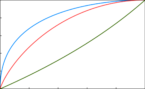
Figure 4: Comparison between $C_{0,{\text{NS}}}$ (green), $C_{\min{\rm E}}$ (red) and $S_{0,{\text{NS}}}$ (blue) for the cq-channel of two pure states, as a function of $0\leq\beta^{2}\leq\frac{1}{2}$.

The largest effort goes into calculating or bounding the numbers $\Upsilon(K^{\otimes n})$ in Eq. (42). In this case we can obtain much better lower bounds (only at most one bit less than optimal value by $n$ uses) compared to Theorem 4.

One copy $n=1$: Let $Q_{i}={\openone}-P_{i}$ be the projection orthogonal to $P_{i}$ (which is rank-one), so that $R_{i}=r_{i}Q_{i}$ with a number $r_{i}\leq s_{i}$. Because of the $Z$-symmetry,

$$ZP_{0}Z=P_{1},ZQ_{0}Z=Q_{1}.$$

We can symmetrize any solution and assume $s_{0}=s_{1}=s$ and $r_{0}=r_{1}=r$. Then the normalization condition reads

$$=s(P_{0}+P_{1})+r(Q_{0}+Q_{1})$$

$$=s(\alpha^{2}|0\rangle\!\langle 0|+\beta^{2}|1\rangle\!\langle 1|)+r(\beta^{2}|0\rangle\!\langle 0|+\alpha^{2}|1\rangle\!\langle 1|),$$

which implies $r=s=1/2$. Hence the maximum value of $\Upsilon(K)=1$.

Many copies $n>1$: In this case it is difficult to find the optimum, but it is enough that we show the achievability of $1/(\alpha^{2n}+\beta^{2n})$ for sufficiently large $n$. Note that this already implies that the SDP for the zero-error number of messages is not multiplicative! Somehow, what’s happening is that the normalization condition of $\sum_{i}(s_{i}P_{i}+R_{i})={\openone}$ is a non-trivial constraint because $R_{i}$ has to be supported on the orthogonal complement of $P_{i}$; this hurts us in the case $n=1$. Now in the case of many copies, $P_{i}$ is a tensor product of single-system projections, hence the orthogonal complement is asymptotically dominating. We have seen how these considerations help in understanding the general case.

We have $2^{n}$ states $P_{i^{n}}=P_{i_{1}}\otimes P_{i_{2}}\otimes\cdots\otimes P_{i_{n}}$, indexed by $n$-bit strings $i^{n}$, which are related by qubit-wise $Z$-symmetry:

$$P_{i^{n}}=Z^{i^{n}}P_{0^{n}}Z^{i^{n}},$$

which motivates that we find $R_{0^{n}}$ (orthogonal to $P_{0^{n}}$) and define

$$R_{i^{n}}\mathrel{\mathop{\mathchar 58\relax}}=Z^{i^{n}}R_{0^{n}}Z^{i^{n}}.$$

Let

$$P^{(n)}_{w}=\sum_{wt(i^{n})=w}|i^{n}\rangle\!\langle i^{n}|,~{}|\Phi_{w}^{(n)}\rangle={n\choose w}^{-1/2}\sum_{wt(i^{n})=w}|i^{n}\rangle,~{}0\leq w\leq n,$$

where $wt(i^{n})$ is the weight (the number of $1$’s) of the $n$-bit string $i^{n}$. We also denote

$$Q_{w}^{(n)}=P^{(n)}_{w}-|\Phi_{w}^{(n)}\rangle\!\langle\Phi_{w}^{(n)}|,$$

which is always a projection for $1\leq w\leq n-1$ and vanishing for $w=0,n$.

For $|\psi_{0}\rangle=\alpha|0\rangle+\beta|1\rangle$, we have

$$|\psi_{0}\rangle^{\otimes n}=\sum_{w=0}^{n}x_{w}|\Phi_{w}^{(n)}\rangle,~{}x_{w}={n\choose w}^{1/2}\alpha^{n-w}\beta^{w}.$$

Clearly

$$Q_{w}^{(n)}|\psi_{0}\rangle^{\otimes n}=0~{}\mbox{and}~{}Q_{w}^{(n)}|\psi_{0}^{\perp}\rangle^{\otimes n}=0,~{}1\leq w\leq n-1$$

for $|\psi_{0}^{\perp}\rangle=\beta|0\rangle-\alpha|1\rangle$.

Now we set all $s_{i^{n}}$ equal to $s$, and propose the following ansatz

$$R_{0^{n}}=s(|\psi_{0}^{\perp}\rangle\!\langle\psi_{0}^{\perp}|)^{\otimes n}+\sum_{w=1}^{n-1}c_{w}Q_{w}^{(n)},$$

where $s$ and $c_{w}$ are non-negative eigenvalues to be determined. Note that $R_{0^{n}}$ is automatically supported on the orthogonal complement of $P_{0^{n}}$.

We need

$$\sum_{i^{n}}(sP_{i^{n}}+R_{i^{n}})={\openone}_{2^{n}},$$

or equivalently,

$$\sum_{i^{n}}Z^{i^{n}}(s(|\psi_{0}\rangle\!\langle\psi_{0}|)^{\otimes n}+s(|\psi_{0}^{\perp}\rangle\!\langle\psi_{0}^{\perp}|)^{\otimes n}+\sum_{w=1}^{n-1}c_{w}Q_{w}^{(n)})Z^{i^{n}}={\openone}_{2^{n}},~{}~{}~{}(*)$$

Using the $Z^{n}$ symmetry, we can calculate

$$\sum_{i^{n}}Z^{i^{n}}(|\psi_{0}\rangle\!\langle\psi_{0}|)^{\otimes n}Z^{i^{n}}=2^{n}\sum_{w=0}^{n}\alpha^{2n-2w}\beta^{2w}P_{w}^{(n)}.$$

Similarly

$$\sum_{i^{n}}Z^{i^{n}}(|\psi_{0}^{\perp}\rangle\!\langle\psi_{0}^{\perp}|)^{\otimes n}Z^{i^{n}}=2^{n}\sum_{w=0}^{n}\alpha^{2w}\beta^{2n-2w}P_{w}^{(n)},$$

and

$$\sum_{i^{n}}Z^{i^{n}}Q_{w}^{(n)}Z^{i^{n}}=2^{n}(1-{n\choose w}^{-1})P_{w}^{(n)}.$$

Applying the property that $\sum_{w=0}^{n}P_{w}^{(n)}={\openone}_{2^{n}}$, we can see that (*) is equivalent to

$$2^{n}s(\alpha^{2n}+\beta^{2n})=1,$$

and

$$2^{n}c_{w}(1-{n\choose w}^{-1})+2^{n}s(\alpha^{2w}\beta^{2n-2w}+\alpha^{2n-2w}\beta^{2w})=1,~{}1\leq w\leq n-1.$$

Then

$$s=2^{-n}(\alpha^{2n}+\beta^{2n})^{-1},~{}\mbox{and}~{}c_{w}=(1-{n\choose w}^{-1})^{-1}s(\alpha^{2n}+\beta^{2n}-\alpha^{2w}\beta^{2n-2w}-\alpha^{2n-2w}\beta^{2w})),1\leq w\leq n-1.$$

We need $R_{0^{n}}\leq s({\openone}_{2^{n}}-P_{0^{n}})$, which is equivalent to $c_{w}\leq s$, or

$$(1-{n\choose w}^{-1})^{-1}\cdot(\alpha^{2n}+\beta^{2n}-\alpha^{2w}\beta^{2n-2w}-\alpha^{2n-2w}\beta^{2w}))\leq 1.$$

The first term of the left hand side (LHS) of the above inequality achieves the maximum when $w=1$, and the second term of the LHS reaches the maximum when $w=\frac{n}{2}$. So we only need

$$(1-{n\choose 1}^{-1})^{-1}(\alpha^{n}-\beta^{n})^{2}\leq 1,$$

or

$$\alpha^{n}-\beta^{n}\leq\sqrt{\frac{n-1}{n}},$$

which is always satisfied when $n$ is large enough. Note that when $n=2$, we have

$$\alpha^{2}-\beta^{2}=|\langle\psi_{0}|\psi_{1}\rangle|\leq\sqrt{\frac{1}{2}}.$$

The above constraint is tight in the sense $\Upsilon(K\otimes K)\geq{1}/(\alpha^{4}+\beta^{4})$ if $|\langle\psi_{0}|\psi_{1}\rangle|\leq\sqrt{\frac{1}{2}}$; otherwise $\Upsilon(K\otimes K)=1$. More precisely, we have $\Upsilon(K\otimes K)=\frac{4}{3}$ when $|\langle\psi_{0}|\psi_{1}\rangle|\leq\sqrt{\frac{1}{2}}$, and $\Upsilon(K\otimes K)>{1}/{(\alpha^{4}+\beta^{4})}$ when $|\langle\psi_{0}|\psi_{1}\rangle|<\sqrt{\frac{1}{2}}$.     $\sqcap$$\sqcup$

Let us consider now the more general case with two output states $\rho_{0}$ and $\rho_{1}$ with projections $P_{0}$ and $P_{1}$, respectively. Denote

$$F_{\max}(\rho_{0},\rho_{1})=F_{\max}(P_{0},P_{1})\mathrel{\mathop{\mathchar 58\relax}}=\max\{|\langle\psi_{0}|\psi_{1}\rangle|\mathrel{\mathop{\mathchar 58\relax}}\psi_{i}\in K_{i},i=0,1\}.$$

$F_{\max}(\rho_{0},\rho_{1})$ is known as the maximal fidelity between $\rho_{0}$ and $\rho_{1}$, but depends only on their supports $K_{0}$ and $K_{1}$. A key property of the maximal fidelity is the following DFY2009 :

Proposition 21

There exists a CPTP map ${\cal T}$ such that ${\cal T}(\rho_{0})=\psi_{0}$ and ${\cal T}(\rho_{1})=\psi_{1}$ if and only if $F_{\max}(\rho_{0},\rho_{1})\leq|\langle\psi_{0}|\psi_{1}\rangle|$.     $\sqcap$$\sqcup$

Applying this result, we can show that the case of two general output states $\rho_{0}$ and $\rho_{1}$ is simply equivalent to the case of two pure output states $\psi_{0}$ and $\psi_{1}$ such that $|\langle\psi_{0}|\psi_{1}\rangle|=F_{\max}(\rho_{0},\rho_{1})$. Thus we have

$$C_{0,{\text{NS}}}(K) =\log{\operatorname{\sf A}}(K)=\log\frac{2}{1+F_{\max}},$$

$$C_{\min{\rm E}}(K) =H\left(\frac{1+F_{\max}}{2},\frac{1-F_{\max}}{2}\right),$$

$$S_{0,{\text{NS}}}(K) =\log\Sigma(K)=1+\sqrt{1-F_{\max}^{2}}.$$

V An operational interpretation of the Lovász number

As we have seen, different non-commutative bipartite graphs $K$, even cq-graphs, having the same confusability graph $G$, can have different assisted zero-error capacity $C_{0,{\text{NS}}}(K)$ and simulation cost $S_{0,{\text{NS}}}(K)$; c.f. the last subsection IV.4 in the previous section.

A classical undirected graph is given by $G=(V,E)$, where $V=\{1,...,n\}$ is the set of vertices, and $E\subset V\times V$ is the set of edges. As shown in previous work DSW2010 , $G$ is naturally associated with a non-commutative graph, denoted $S_{G}$, via the following way:

$$S_{G}={\rm span}\{|i\rangle\!\langle j|\mathrel{\mathop{\mathchar 58\relax}}i\sim j\},$$ (46)

where $i\sim j$ means confusability: $i=j$ or $\{i,j\}\in E$ is an edge of the graph Lovasz1979 .

Hence the questions we are facing are the maximum and minimum $C_{0,{\text{NS}}}(K)$ and $S_{0,{\text{NS}}}(K)$ over all cq-graphs $K$ with $K^{\dagger}K<S_{G}$. While the maximum is clearly $\log|B|$ for both quantities, the minima turn out to be much more interesting. We restate here the main result we will go on to prove in this section.

Theorem 5 For any classical graph $G$, the Lovász number $\vartheta(G)$ is the minimum zero-error classical capacity assisted by quantum no-signalling correlations of any cq-channels that have $G$ as non-commutative graph, i.e.

$$\log\vartheta(G)=\min\bigl{\{}C_{0,{\rm NS}}(K)\mathrel{\mathop{\mathchar 58\relax}}K^{\dagger}K<S_{G}\bigr{\}},$$

where the minimization is over cq-graphs $K$.
In particular, equality holds for any cq-channel $i\rightarrow|\psi_{i}\rangle\!\langle\psi_{i}|$ such that $\{|\psi_{i}\rangle\}$ is an optimal orthogonal representation for $G$ in the sense of Lovász’ original definition Lovasz1979 .

The proof of this result is achieved by combining two facts about the semidefinite packing number for cq-channels: 1) ${\operatorname{\sf A}}(K)$ gives the zero-error classical capacity assisted with no-signaling correlations for a cq-channel; 2) the Lovász number $\vartheta(G)$ of a graph is given by the minimization of ${\operatorname{\sf A}}(K)$ for all non-commutative bipartite graph $K$ that generate the same confusability graph $G$. The first fact has been proven in Theorem 16, so we focus on the second for the rest of the section.

Let $K=\operatorname{span}\{E_{i}\mathrel{\mathop{\mathchar 58\relax}}1\leq i\leq n\}$ be a Kraus operator space with $\operatorname{Tr}(E_{i}^{\dagger}E_{j})=\delta_{ij}$, and let $|\Phi\rangle=\sum_{i=1}^{d}|i\rangle|i\rangle$ be the non-normalized maximally entangled state. Then $P$, the projection on the support of the Choi-Jamiołkowski state, can be written as

$$P_{AB}=\sum_{i=1}^{n}({\openone}\otimes E_{i})|\Phi\rangle\!\langle\Phi|({\openone}\otimes E_{i})^{\dagger}.$$ (47)

We can rewrite the semidefinite packing number ${\operatorname{\sf A}}(K)$ using these Kraus operators $\{E_{i}\}$:

$${\operatorname{\sf A}}(K)=\max\operatorname{Tr}R\ \text{s.t. }\ \sum_{i=1}^{n}E_{i}RE_{i}^{\dagger}\leq{\openone}_{B},\ R\geq 0.$$ (48)

Note that $\{E_{i}\}$ spans a valid Kraus operator space of a quantum channel. So $\sum_{i}E_{i}^{\dagger}E_{i}>0$ (positive definite). The dual SDP is

$${\operatorname{\sf A}}(K)=\min\operatorname{Tr}T\ \text{ s.t. }\ \sum_{i=1}^{n}E_{i}^{\dagger}TE_{i}\geq{\openone}_{A},\ T\geq 0,$$ (49)

and we can easily verify that both the primal and the dual are strictly feasible by choosing $R=0$ and $T=\lambda{\openone}_{B}$ (here $\lambda>0$ is sufficiently large), respectively. Hence strong duality holds.

We will start by deriving some minimax representations of ${\operatorname{\sf A}}(K)$. Let us introduce

$$\widehat{{\operatorname{\sf A}}}(K)\mathrel{\mathop{\mathchar 58\relax}}=\min_{\rho}\lambda_{\max}({\cal N}(\rho)) =\min_{\rho}\max_{\sigma}\operatorname{Tr}({\cal N}(\rho)\sigma)$$

$$=\max_{\sigma}\min_{\rho}\operatorname{Tr}({\cal N}^{\dagger}(\sigma)\rho)$$

$$=\max_{\sigma}\lambda_{\min}\bigl{(}{\cal N}^{\dagger}(\sigma)\bigr{)}.$$

where $\lambda_{\max}(T)$ and $\lambda_{\min}(T)$ represent the maximal and the minimal eigenvalues of a Hermitian operator $T$, respectively, and ${\cal N}(\rho)=\sum_{i}E_{i}\rho E_{i}^{\dagger}$, ${\cal N}^{\dagger}(\sigma)=\sum_{i}E_{i}^{\dagger}\sigma E_{i}$ are CP maps (but not necessarily trace or unit preserving); $\rho$ and $\sigma$ range over all density operators, i.e. $\rho,\sigma\geq 0$ and $\operatorname{Tr}\rho=\operatorname{Tr}\sigma=1$.

In the second and the fourth equalities above, we have employed the following well-known characterizations:

$$\lambda_{\max}(T)=\max_{\rho}\operatorname{Tr}\rho T\ \text{and}\ \lambda_{\min}(T)=\min_{\sigma}\operatorname{Tr}\sigma T.$$

In the third equality we have employed the obvious equality $\operatorname{Tr}({\cal N}(\rho)\sigma)=\operatorname{Tr}(\rho N^{\dagger}(\sigma))$, and von Neumann’s minimax theorem Sion:minimax , since $\operatorname{Tr}{\cal N}(\rho)\sigma$ is a linear function with respect to $\rho$ and $\sigma$, and $\rho$ and $\sigma$ range over convex compact sets.

Lemma 22

Under the above definitions,

$${\operatorname{\sf A}}(K)=\frac{1}{\widehat{{\operatorname{\sf A}}}(K)},$$

for any non-commutative bipartite graph $K$.

Proof.

Suppose that ${\operatorname{\sf A}}(K)=\operatorname{Tr}R_{0}$ for some $R_{0}\geq 0$. Let us construct a density operator $\rho_{0}=\frac{R_{0}}{\operatorname{Tr}R_{0}}$. By the assumption $\sum_{i}E_{i}R_{0}E_{i}^{\dagger}\leq{\openone}_{B}$, we have

$$\sum_{i}E_{i}\rho_{0}E_{i}^{\dagger}\leq\frac{1}{\operatorname{Tr}R_{0}}{\openone}_{B},$$

or equivalently

$${\cal N}(\rho_{0})\leq\frac{1}{{\operatorname{\sf A}}(K)}{\openone}_{B}.$$

By the definition of $\widehat{{\operatorname{\sf A}}}(K)$, we have

$$\widehat{{\operatorname{\sf A}}}(K)\leq\lambda_{\max}({\cal N}(\rho_{0}))\leq\frac{1}{{\operatorname{\sf A}}(K)}.$$

Conversely, suppose that $\widehat{{\operatorname{\sf A}}}(K)=\lambda_{\max}({\cal N}(\rho_{0}))$ for some density operator $\rho_{0}$. Then we have ${\cal N}(\rho_{0})\leq\widehat{{\operatorname{\sf A}}}(K){\openone}_{B}$, and thus

$${\cal N}\bigl{(}\rho_{0}/\widehat{{\operatorname{\sf A}}}(K)\bigr{)}\leq{\openone}_{B}.$$

That means $\rho_{0}/\widehat{{\operatorname{\sf A}}}(K)$ is a feasible solution of the SDP defining the semidefinite packing number. By the definition of ${\operatorname{\sf A}}(K)$, we know that

$${\operatorname{\sf A}}(K)\geq\operatorname{Tr}\rho_{0}/\widehat{{\operatorname{\sf A}}}(K)=\frac{1}{\widehat{{\operatorname{\sf A}}}(K)},$$

concluding the proof.     $\sqcap$$\sqcup$

Focussing on the special class of cq-channels, which are in some sense the direct quantum generalizations of classical channels, we are now ready for

Proof of Theorem 5  Let $K$ correspond to a cq-channel $i\mapsto\rho_{i}$, and let $P_{i}$ be the projection on the support of quantum states $\rho_{i}$. It will be more convenient to study $\widehat{{\operatorname{\sf A}}}(K)$ instead of ${\operatorname{\sf A}}(K)$. Actually, applying the above minimax representation to this special case, we have

$$\widehat{{\operatorname{\sf A}}}(K)=\min_{\{t_{i}\}}\max_{\sigma}\operatorname{Tr}\sigma\left(\sum_{i}t_{i}P_{i}\right)=\max_{\sigma}\min_{\{t_{i}\}}\operatorname{Tr}\sigma\left(\sum_{i}t_{i}P_{i}\right)=\max_{\sigma}\min_{i}\operatorname{Tr}\sigma P_{i},$$

where $\{t_{i}\}$ ranges over probability distributions, and $\sigma$ ranges over density operators. The right-most expression motivates us to introduce some notations.

By definition, $\{P_{i}\}$ is an orthogonal representation (OR) of the confusability graph $G$ induced by the cq-channel. The value of an OR $\{P_{i}\}$ is defined as follows:

$$\eta(\{P_{i}\})=\max_{\sigma}\min_{i}\operatorname{Tr}P_{i}\sigma.$$

We introduce the following function of a graph $G$,

$$\eta(G)=\max_{\{P_{i}\}}\eta(\{P_{i}\}),$$

where the maximization ranges over all possible ORs of $G$. Clearly, if we require that an OR consists of only rank-one projections and $\sigma$ takes only rank-one projection, then $\eta(G)=\vartheta(G)^{-1}$, the reciprocal of the Lovász number of $G$ Lovasz1979 . It has been shown in CSW2010 that even allowing $P_{i}$ to be general projection but $\sigma$ to be rank-one projection, there is no difference between $\eta(G)$ and $\vartheta(G)^{-1}$. However, if $\sigma$ is a mixed state, we can only have $\eta(G)\geq\vartheta(G)^{-1}$. Interestingly, we can show that equality does hold. In fact, it is evident that if $\{P_{i}\}$ is an OR for a graph $G$, then $\{P_{i}\otimes{\openone}_{B}\}$ remains an OR for the same graph, where $B$ is any auxiliary system. Now the value of $\{P_{i}\}$ with respect to general mixed states, is the same as the value of $\{P_{i}\otimes{\openone}_{B}\}$ with respect to pure states. That is,

$$\max_{\sigma}\min_{i}\operatorname{Tr}P_{i}\sigma=\max_{\Psi}\min_{i}\operatorname{Tr}((P_{i}\otimes{\openone}_{B})|\Psi_{AB}\rangle\langle\Psi_{AB}|),$$

where $\sigma=\operatorname{Tr}_{B}|\Psi_{AB}\rangle\langle\Psi_{AB}|$. The above equality follows directly from the fact that

$$\operatorname{Tr}P_{i}\sigma=\operatorname{Tr}((P_{i}\otimes{\openone}_{B})|\Psi_{AB}\rangle\langle\Psi_{AB}|),$$

where $|\Psi_{AB}\rangle$ is any purification of $\sigma$.

Summarizing, we have

$$\min_{K}{\operatorname{\sf A}}(K)=\min_{K}\frac{1}{\widehat{{\operatorname{\sf A}}}(K)}=\frac{1}{\eta(G)}=\vartheta(G),$$

and we are done.     $\sqcap$$\sqcup$

As a final comment on the above proof, note that for a fixed OR $\{P_{i}\}$, we cannot always choose the optimal handle $\sigma$ as a pure state– the restriction to rank-one projectors and pure state handle only emerges as we optimize over both elements.

We would like to interpret Theorem 5 to say intuitively that the zero-error capacity of a graph $G$ assisted by no-signalling correlations is $\vartheta(G)$. The problematic part of such a manner of speaking is that there are many cq-graphs $K$ with the same confusability graph $G$, but the no-signalling assisted capacity may vary with these $K$.

However, note that for any (finite) family of cq-graphs $K^{(\alpha)}$ such that ${K^{(\alpha)}}^{\dagger}K^{(\alpha)}=S_{G}$, $K^{(\alpha)}=\sum_{i}|i\rangle\otimes K_{i}^{(\alpha)}$, we can construct a cq-graph $K$ that “dominates” all of the $K^{(\alpha)}$ in the sense that any no-signalling assisted code for $K$ can be used directly for $K^{(\alpha)}$ because actually $K^{(\alpha)}<K$:

$$K=\sum_{i}|i\rangle\otimes K_{i},\quad K_{i}=\bigoplus_{\alpha}K_{i}^{(\alpha)}.$$

By going from direct sums to direct integrals, we can thus construct a universal cq-graph

$$\widetilde{K}(G)=\sum_{i}|i\rangle\otimes\widetilde{K}_{i}$$

which dominates all $K^{(\alpha)}$ with confusability graph $G$, in fact contains them up to isomorphism. Any no-signalling assisted code for this object will deal in particular with every eligible channel simultaneously. The only caveat is that the $\widetilde{K}_{i}$ are subspaces in an a priori infinite dimensional Hilbert space, and all of our proofs (in particular that of Theorem 4) require finite dimension as a technical condition. We conjecture however that the capacity result of Theorem 4 still holds in that setting.

Minimum simulation cost of a confusability graph. Just as we were looking at the smallest zero-error capacity over all cq-channels with a given confusability graph $G$ in this section, we can study the minimum simulation cost over all cq-graphs $K$ with $K^{\dagger}K<S_{G}$. To be precise, we are interested in

$$\Sigma(G)\mathrel{\mathop{\mathchar 58\relax}}=\inf\{\Sigma(K)\mathrel{\mathop{\mathchar 58\relax}}K\text{ cq-graph with }K^{\dagger}K<S_{G}\},$$

and the asymptotic simulation cost (regularization)

$$S_{0,{\text{NS}}}(G)\mathrel{\mathop{\mathchar 58\relax}}=\lim_{n\rightarrow\infty}\frac{1}{n}\log\Sigma(G^{n}),$$

where $G^{n}=G\times\cdots\times G$ denotes the $n$-fold strong graph product. The latter limit exists and equals the infimum because evidently $\log\Sigma(G\times H)\leq\log\Sigma(G)+\log\Sigma(H)$.

For a cq-graph $K$, we have

$$\log{\operatorname{\sf A}}(K)\leq C_{\min E}(K)\leq\log\Sigma(K),$$ (50)

in fact for every eligible cq-channel ${\cal N}$ with non-commutative bipartite graph $K$,

$$\log{\operatorname{\sf A}}(K)\leq C({\cal N})=C_{E}({\cal N})\leq\log\Sigma({\cal N}).$$

The reason is that $\log{\operatorname{\sf A}}(K)=C_{0,{\text{NS}}}(K)$ is the zero-error capacity assisted by no-signalling correlations (Theorem 4); while $C_{E}({\cal N})=C({\cal N})$ is the Holevo (small-error) capacity, which is the same as the entanglement-assisted capacity for cq-channels and which is not increased by any other available no-signalling resources because of the Quantum Reverse Shannon Theorem BDHS+2009 ; QRST-simple ; and $\log\Sigma({\cal N})=-H_{\min}(X|B)_{J}$ is the perfect simulation cost of the channel when assisted by no-signalling resources, with the Choi-Jamiołkowski matrix $J=\sum_{i}|i\rangle\!\langle i|\otimes P_{i}$, Eq. (5).

In Eq. (50), $C_{\rm\min E}(K)=C_{\min}(K)$ because $K$ is a cq-graph, so we only need to consider cq-channels ${\cal N}\mathrel{\mathop{\mathchar 58\relax}}i\mapsto\rho_{i}$ in the minimization, for which

$$C_{\rm E}({\cal N})=C({\cal N})=\max_{P_{X}}I(X\mathrel{\mathop{\mathchar 58\relax}}B)=\max_{P_{X}}S\left(\sum_{i}P_{X}(i)\rho_{i}\right)-\sum_{i}P_{X}(i)S(\rho_{i}).$$

Letting now

$$C_{\min}(G)\mathrel{\mathop{\mathchar 58\relax}}=\inf\{C_{\min}(K)\mathrel{\mathop{\mathchar 58\relax}}K\text{ cq-graph with }K^{\dagger}K<S_{G}\},$$

we then have the following additivity result.

Lemma 23

For any two graphs $G$ and $H$,

$$C_{\min}(G\times H)=C_{\min}(G)+C_{\min}(H).$$

Proof.

The subadditivity, $C_{\min}(G\times H)\leq C_{\min}(G)+C_{\min}(H)$, is evident from the definition, because if $K^{\dagger}K<S_{G}$ and $L^{\dagger}L<S_{H}$, then $(K\otimes L)^{\dagger}(K\otimes L)<S_{G\times H}$.

It remains to show the opposite inequality “$\geq$”. This relies crucially on the minimax identity

$$C_{\min}(G)=\inf_{{\cal N}}\max_{P_{X}}I(X\mathrel{\mathop{\mathchar 58\relax}}B)=\max_{P_{X}}\inf_{{\cal N}}I(X\mathrel{\mathop{\mathchar 58\relax}}B),$$ (51)

where the maximum is over probability distributions $P_{X}$ and the infimum is over cq-channels ${\cal N}$ with confusability graph contained in $G$. This is a special case of Sion’s minimax theorem Sion:minimax , since the Holevo mutual information is well-known to be concave in $P_{X}$ and convex in ${\cal N}$, while the domain of $P_{X}$ is the convex compact simplex of finite probability distributions and the domain of ${\cal N}$ is an infinite-dimensional convex set.

Now, for a cq-channel ${\cal N}\mathrel{\mathop{\mathchar 58\relax}}ij\mapsto\rho_{ij}$ with confusability graph contained in $G\times H$, and an arbitrary distribution $P_{XY}$ of the two input variables $X$ and $Y$, we have

$$I(XY\mathrel{\mathop{\mathchar 58\relax}}B)=I(X\mathrel{\mathop{\mathchar 58\relax}}B)+I(Y\mathrel{\mathop{\mathchar 58\relax}}B|X)=I(X\mathrel{\mathop{\mathchar 58\relax}}B)+\sum_{i}P_{X}(i)I(Y\mathrel{\mathop{\mathchar 58\relax}}B|X=i).$$ (52)

Here, the first term refers to the cq-channel

$$\overline{{\cal N}}\mathrel{\mathop{\mathchar 58\relax}}i\mapsto\overline{\rho}_{i}=\sum_{j}P_{Y|X}(j|i)\rho_{ij},$$

while the $i$-th summand in the second term sum refers to the cq-channel

$${\cal N}_{i}\mathrel{\mathop{\mathchar 58\relax}}j\mapsto\rho_{ij}.$$

Note that $\overline{{\cal N}}$ is eligible for $G$ (since $i\not\sim i^{\prime}$ implies $ij\not\sim i^{\prime}j^{\prime}$ for all $j,j^{\prime}$, hence $\rho_{ij}\perp\rho_{i^{\prime}j^{\prime}}$), while similarly for all $i$, ${\cal N}_{i}$ is eligible for $H$. Thus, in Eq. (52), we can take the infimum over eligible cq-channels, to obtain

$$\inf_{{\cal N}}I(XY\mathrel{\mathop{\mathchar 58\relax}}B)\geq\inf_{{\cal M}_{1}}I(X\mathrel{\mathop{\mathchar 58\relax}}C_{1})+\inf_{{\cal M}_{2}}I(Y\mathrel{\mathop{\mathchar 58\relax}}C_{2})=\inf_{{\cal M}_{1},{\cal M}_{2}}I(X^{\prime}Y^{\prime}\mathrel{\mathop{\mathchar 58\relax}}C_{1}C_{2}),$$

where the minimizations are over cq-channels ${\cal N}$ eligible for $G\times H$, ${\cal M}_{1}$ eligible for $G$ and ${\cal M}_{2}$ eligible for $H$, whereas $X^{\prime}$ and $Y^{\prime}$ are independent copies of $X$ and $Y$, i.e. they are jointly distributed according to $P_{X}\times P_{Y}$. Now, taking the maximum over distributions $P_{XY}$ completes the proof because of the minimax formula (51).     $\sqcap$$\sqcup$

As a corollary, we get the following chain of inequalities:

$$\log\vartheta(G)\leq C_{\min}(G)\leq S_{0,{\text{NS}}}(G)\leq\log\Sigma(G)\leq\log\alpha^{*}(G).$$ (53)

Note that it may be true that $S_{0,{\text{NS}}}(G)=\log\Sigma(G)$, but to prove this we would need to show the additivity relation $\log\Sigma(G\times H)=\log\Sigma(G)+\log\Sigma(H)$, which remains unknown. Another observation is that if in the respective minimizations, the channels are restricted to classical channels, then the results of CLMW2011 show that

$$\min_{K}\log{\operatorname{\sf A}}(K)=\min_{{\cal N}}C({\cal N})=\min_{{\cal N}}\Sigma({\cal N})=\log\alpha^{*}(G).$$

We now demonstrate by example that the rightmost inequality in (53) can be strict, when quantum channels are considered. Namely, for even $n$ let $G=\overline{H_{n}}$ the complement of the Hadamard graph $H_{n}$, whose vertices are the vectors $\{\pm 1\}^{n}$ and two vectors $v,w$ are adjacent in $H_{n}$ if and only if they are orthogonal in the Euclidean sense, $v^{\top}w=0$. In other words, the cq-channel ${\cal N}\mathrel{\mathop{\mathchar 58\relax}}v\mapsto\frac{1}{n}|v\rangle\!\langle v|$ has confusability graph $G$. Since the output dimension is $n$, we see from this that $\Sigma(G)\leq\Sigma({\cal N})\leq n$, which happens to coincide with the Lovász number, $\vartheta(G)=n$, hence $\log\vartheta(G)=C_{\min}(G)=S_{0,{\text{NS}}}(G)=\log\Sigma(G)=\log n$. On the other hand, the clique number of $G$ is known to be upper bounded $\omega(G)\leq 1.99^{n}$ FranklRoedl , hence $\alpha^{*}(G)\geq\frac{|G|}{\omega(G)}\geq 1.005^{n}$, meaning $\log\alpha^{*}(G)\geq\Omega(n)$.

We think that also the leftmost inequality in (53) can be strict. But although the pentagon $G=C_{5}$ seems to be a candidate, for which we conjecture (based on some ad hoc calculations) that $C_{\min}(G)=S_{0,{\text{NS}}}(G)=\log\Sigma(G)=\log\alpha^{*}(G)=\log\frac{5}{2}$, whereas $\log\vartheta(G)=\frac{1}{2}\log 5$, a rigorous proof of this has so far eluded us.

Whether the other two inequalities can be strict remains an open question.

VI Feasibility of zero-error communication via general non-commutative bipartite graph assisted by quantum no-signalling correlations

Given a non-commutative bipartite graph $K$, it is important to know when $K$ is able to send classical information exactly in the presence of quantum no-signalling correlations. It turns out that these channels can be precisely characterized; we will start with cq-graphs.

Theorem 24

Let $K$ be a non-commutative bipartite cq-graph specified by a set of projections $\{P_{i}\mathrel{\mathop{\mathchar 58\relax}}1\leq i\leq n\}$ with supports $K_{i}=\operatorname{supp}P_{i}$. Then the following are equivalent:

1. $C_{0,{\rm NS}}(K)>0$;

2. ${\operatorname{\sf A}}(K)>1$;

3. $\bigcap_{i}K_{i}=\{0\}$.

Proof.

The equivalence of i) and ii) follows directly from Proposition 16.

The equivalence of ii) and iii) is only a simple application of the SDP of ${\operatorname{\sf A}}(K)$ for bipartite cq-graphs. First, we show that iii) implies ii). By contradiction, assume that the intersection of supports of $P_{i}$ is empty while ${\operatorname{\sf A}}(K)=1$. Recall that the dual SDP of ${\operatorname{\sf A}}(K)$ is given by

$${\operatorname{\sf A}}(K)=\min\operatorname{Tr}T\ \text{ s.t. }\ \operatorname{Tr}P_{i}T\geq 1,\ T\geq 0,1\leq i\leq n.$$

Then ${\operatorname{\sf A}}(K)=1$ implies that we can find $T_{0}\geq 0$ such that $\operatorname{Tr}T_{0}=1$ and $\operatorname{Tr}P_{i}T_{0}\geq 1$ for any $i$. Clearly $T_{0}$ is a density operator, and we should have $\operatorname{Tr}P_{i}T_{0}=1$ for any $i$. The only possibility is that $T_{0}$ is in the intersection of the supports of $P_{i}$, which is a contradiction. Now we turn to show that ii) implies iii). Again by contradiction, assume that ${\operatorname{\sf A}}(K)>1$ while the intersection of supports is nonempty. Then we can find a pure state $|\psi\rangle$ from the intersection such that $P_{i}\geq|\psi\rangle\!\langle\psi|$. So

$${\openone}\geq\sum_{i}s_{i}P_{i}\geq\left(\sum_{i}s_{i}\right)|\psi\rangle\!\langle\psi|,$$

thus any feasible solution should have $\sum_{i}s_{i}\leq 1$, which indeed implies that ${\operatorname{\sf A}}(K)=1$.     $\sqcap$$\sqcup$

Theorem 25

Let $K$ be a non-commutative bipartite graph with Choi-Jamiołkowski projection $P_{AB}$, and let $Q_{AB}={\openone}_{AB}-P_{AB}$ be the orthogonal complement of $P_{AB}$. Then the following are equivalent:

1. $C_{0,{\rm NS}}(K)>0$;

2. ${\operatorname{\sf A}}(K)>1$;

3. $\operatorname{Tr}_{A}P_{AB}<d_{A}{\openone}_{B}$;

4. $\operatorname{Tr}_{A}Q_{AB}$ is positive definite.

As a matter of fact, we have

$$C_{0,{\rm NS}}(K)\geq\log\frac{d_{A}}{\|\operatorname{Tr}_{A}P_{AB}\|_{\infty}}\quad\text{and}\quad{\operatorname{\sf A}}(K)\geq\frac{d_{A}}{\|\operatorname{Tr}_{A}P_{AB}\|_{\infty}}.$$

Proof.

The meaning of i) and ii) are very clear, while iii) and iv) need some explanation.

Essentially, iv) means we can find a CP map from $B$ to $A$ with Choi-Jamiołkowski matrix $V_{AB}$ supporting on some subset of $Q_{AB}$. Note that in the one-shot SDP formulation of $\Upsilon(K)$, we need $V_{AB}$ to be a CPTP map. However, the trace-preserving condition is not necessary for asymptotic case but only $\operatorname{Tr}_{A}V_{AB}$ is positive definite, which is the most nontrivial part of this theorem.

iii) is directly equivalent to iv) as we have $P_{AB}+Q_{AB}={\openone}_{AB}$, hence

$$\operatorname{Tr}_{A}P_{AB}+\operatorname{Tr}_{A}Q_{AB}=d_{A}{\openone}_{B}.$$

In the following we only focus on i), ii), and iii). The equivalence of ii) and iii) is straightforward, simply noticing that ${\openone}_{A}/\|P_{B}\|_{\infty}$ is a feasible solution to the primal SDP for ${\operatorname{\sf A}}(K)$, where $P_{B}=\operatorname{Tr}_{A}P_{AB}$.

The equivalence of i) and iii) is much more difficult and non-trivial. In the following we want to explain a little bit more about this equivalence as there are some tricky points.

First, let’s see how to use iii) to derive i). We can apply the standard super-dense coding protocol, and obtain a cq-channel with $d_{A}^{2}$ outputs $\{(U_{m}\otimes{\openone}_{B})J_{AB}(U_{m}\otimes{\openone}_{B})^{\dagger}\}$, and the projections are given by $\{(U_{m}\otimes{\openone}_{B})P_{AB}(U_{m}\otimes{\openone}_{B})^{\dagger}\}$, where $U_{m}$ are generalized Pauli matrices acting on $A$. So we can compute the semidefinite packing number as

$$\frac{d_{A}^{2}}{\sum_{m=1}^{d_{A}^{2}}(U_{m}\otimes{\openone}_{B})P_{AB}(U_{m}\otimes{\openone}_{B})^{\dagger}}=\frac{d_{A}}{\|P_{B}\|_{\infty}}.$$ (54)

This is also the zero-error no-signalling assisted classical capacity of this cq-channel. Noticing that when $P_{B}<d_{A}{\openone}_{B}$ strictly holds, the right-hand side of the above equation is strictly larger than $1$.

The fact that i) implies iii) can be proven by contradiction together with the one-shot SDP formulation for $\Upsilon(K)$. Assume i) holds but $Q_{B}$ does not have full rank. Then we can find a non-zero vector $|x\rangle_{B}$ such that $Q_{B}|x\rangle=0$. Or equivalently, $Q_{AB}({\openone}_{A}\otimes|x\rangle\!\langle x|_{B})=0$.

i) means for some $n>1$ we have $\Upsilon(K^{\otimes n})>1$. By the one-shot SDP formulation of $\Upsilon(K^{\otimes n})$, we can find positive semidefinite operators $S_{A^{n}}$ and $E_{A^{n}B^{n}}$, such that

$$\operatorname{Tr}S_{A^{n}}>1,S_{A^{n}}\otimes{\openone}_{B^{n}}\geq E_{A^{n}B^{n}}\geq 0,\operatorname{Tr}_{A^{n}}E_{A^{n}B^{n}}={\openone}_{B^{n}},\ \text{and}\ \operatorname{Tr}P_{AB}^{\otimes n}(S_{A^{n}}\otimes{\openone}_{B^{n}}-E_{A^{n}B^{n}})=0.$$

So we can find $F_{A^{n}B^{n}}=S_{A^{n}}\otimes{\openone}_{B^{n}}-E_{A^{n}B^{n}}$ with $\operatorname{Tr}_{A^{n}}F_{A^{n}B^{n}}=(\operatorname{Tr}S-1){\openone}_{B^{n}}$, with full rank. On the other hand, we also have $F_{A^{n}B^{n}}$ supported on ${\openone}_{A^{n}B^{n}}-P_{AB}^{\otimes n}$, and the later is the summation of product terms such as $P_{AB}\otimes Q_{AB}\otimes\cdots\otimes P_{AB}$, containing at least one factor $Q_{AB}$ each. So we have

$$F_{A^{n}B^{n}}({\openone}_{A^{n}}\otimes|x\rangle\!\langle x|^{\otimes n}_{B^{n}})=0,$$

which immediately implies that $F_{B^{n}}=\operatorname{Tr}_{A^{n}}F_{A^{n}B^{n}}$ is vanishing on the product vector $|x\rangle^{\otimes n}_{B^{n}}$, contradicting the fact that $F_{B}$ has full rank.     $\sqcap$$\sqcup$

The simple bound $\frac{d_{A}}{\|\operatorname{Tr}_{A}P_{AB}\|_{\infty}}$ is very interesting, and in some important cases it is tight, such as the cq-channels with symmetric outputs, and the class of Pauli channels. It would be interesting to know whether this kind of “entanglement-assisted coding” could provide a possible way to resolve our puzzle between $C_{0,{\text{NS}}}(K)$ and ${\operatorname{\sf A}}(K)$, eventually.

VII Conclusion and open problems

We have shown that there is a meaningful theory of zero-error communication via quantum channels when assisted by quantum no-signalling correlations.

In the terminology of non-commutative graph theory, both the one-shot zero-error classical capacity and simulation cost for non-commutative bipartite graphs assisted by quantum no-signalling correlations have been formulated into feasible SDPs. The asymptotic problems for non-commutative bipartite cq-graphs have also been successfully solved, where the capacity turns out to involve a nontrivial regularization of super-multiplicative SDPs, which nevertheless leads to another SDP, the semidefinite packing number. We found analogously that the zero-error simulation cost of a cq-graph is given by a semidefinite covering number, which in contrast to the classical case is in general larger than the packing number.

The zero-error classical capacity of a classical graph assisted by quantum no-signalling correlations is given precisely by the celebrated Lovász number. For the most general non-commutative bipartite graphs, we are able to provide a necessary and sufficient condition for when these graphs have positive zero-error classical capacity assisted with quantum no-signalling correlations

We know rather little about the asymptotic capacity and simulation cost for non-commutative bipartite graphs that are not classical-quantum, however. A very interesting candidate is the non-commutative bipartite graph $K(r)=\operatorname{span}\{E_{0},E_{1}\}$ associated with the amplitude damping channel ${\cal N}=\sum_{i=0}^{1}E_{i}\cdot E_{i}^{\dagger}$ , with $E_{0}=|0\rangle\!\langle 0|+\sqrt{1-r}|1\rangle\!\langle 1|$, $E_{1}=\sqrt{r}|0\rangle\!\langle 1|$ and $0\leq r\leq 1$. The extremes $r=0$ and $r=1$ correspond to the noiseless qubit channel and a constant channel, respectively, and are trivial; we will hence assume $0<r<1$. This channel is quite interesting because it gives a separation between the semidefinite packing number and the modified version, and other quantities. It is also interesting because there is only one unique channel ${\cal N}_{r}$ which has $K(r)$ as the Kraus operator space. Actually it is a non-unital extreme point of the convex set of CPTP maps. This channel is also able to communicate classical information without error when assisted with no-signalling correlations. By applying the above super-dense coding bound, we have

$$C_{0,{\text{NS}}}(K_{r})\geq\log\frac{4-2r}{3-r}.$$

By some routine calculation, we can show that the semidefinite packing number is ${\operatorname{\sf A}}(K_{r})=2-r$, the revised version $\widetilde{{\operatorname{\sf A}}}(K_{r})=(2-r)^{2}$, and

$$C_{\min{\rm E}}(K_{r})=\max_{0\leq p\leq 1}H_{2}(p)+H_{2}(rp)-H_{2}((1-r)p),$$

where $H_{2}(x)=-x\log x-(1-x)\log(1-x)$ is the binary entropy. Clearly, $C_{\min{\rm E}}(K_{0.5})=1$, while $\widetilde{{\operatorname{\sf A}}}(K_{0.5})=2.25>2$. This means that the revised semidefinite packing number cannot be equal to the zero-error classical capacity assisted by quantum no-signalling correlations. Whether the original form has the same problem remains unknown.

There are many other interesting open problems, of which we highlight a few here. First, it would be very interesting to explore the mathematical structures of quantum no-signalling correlations in greater detail, and to characterize quantitatively how much non-locality is contained in a quantum no-signalling correlation.

Second, it is of great importance to solve the general asymptotic capacity and cheapest simulation problems in the zero-error setting when assisted with quantum no-signalling correlations. In particular, are there examples of strict sub-multiplicativity of $\Sigma(K)$?

The third problem of great interest is to explore the relationship between the quantum Lovász $\vartheta$ function introduced in Ref. DSW2010 for a non-commutative graph $S$, and the zero-error classical capacity of this non-commutative graph assisted with quantum no-signalling correlations, i.e. of Kraus operator spaces $K$ with $K^{\dagger}K<S$. Likewise, what is the minimum simulation cost $\Sigma(K)$ or $S_{0,\text{NS}}(K)$ over all such $K$? This latter is open already for a classical graph $G$ and cq-graphs $K$ with confusability graph $G$, see the end of section V. In any case, it seems that $\Sigma(G)$ and $2^{C_{\min}(G)}$ are two new interesting, multiplicative graph parameters, different from both $\vartheta(G)$ and $\alpha^{*}(G)$.

Fourth: Are no-signalling correlations really necessary to achieve the asymptotic simulation cost $S_{0,{\text{NS}}}(K)$, or is perhaps entanglement enough? The motivation for this question comes from CLMW2011 where it was shown that for classical channels, optimal asymptotic simulation is possible using only shared randomness, no other non-local resources are needed. A nice test case for this question is provided by cq-graphs, for which it is easy to see that $S_{0,{\text{NS}}}(K)\leq\log|B|$. On the other hand, the entanglement-assisted simulation of cq-channels, also known as remote state preparation Lo ; rsp is far harder to understand. Indeed, for generic channels the best known protocol requires $2\log|B|$ bits of communication, which is the communication cost of teleportation tele ; Lo .

Fifth, which no-signalling resources are actually required to achieve the asymptotic zero-error capacity $C_{0,{\text{NS}}}(K)$? This seems an innocuous question – after all, for each channel the SDP $\Upsilon(K)$ tells us precisely which no-signalling correlation achieves the maximum. But looking at the case of classical channels and bipartite graphs CLMW2010 , in the light of a classical result of Elias Elias:list , shows that there only a very specific resource is required, which is universal for all channels. Namely, according to (Elias:list, , Prop. 4), a list size-$L$ list code for a bipartite graph $\Gamma$ can achieve a rate $R=\left(1-\frac{1}{L}\right)\log\alpha^{*}(\Gamma)-O\left(\frac{1}{L}\right)$, which is arbitrarily close to $\log\alpha^{*}(\Gamma)$ for sufficiently large $L$. Using such a code, Alice can send a message $i$ out of $M=\lfloor 2^{nR}\rfloor$ over $n$ uses of the channel, and Bob will end up with a list, i.e. a subset $I\subset 2^{[M]}$ of $|I|=L$ possible messages such that $i\in I$. To resolve the remaining ambiguity, Alice and Bob now require a no-signalling resource $S_{{M\choose L}}=S(\alpha\beta|iI)$ that we call subset correlation, defined for $i\in[M]$, $I\in{[M]\choose L}$, $t,u\in[L]$, with

$$S(tu|iI)=\begin{cases}\frac{1}{L}&\text{ if }i=i_{s}\in I=\{i_{1}<\ldots<i_{L}\}\ \&{}\ u-t=s\mod L,\\ \frac{1}{L}&\text{ if }i=i_{s}\in I=\{i_{1}<\ldots<i_{L}\}\ \&{}\ u-t\neq s\mod L,\\ \frac{1}{L^{2}}&\text{ if }i\not\in I.\end{cases}$$

Alice will input $i$ into the box, Bob the set $I$, and then Alice will send her output $t$ to Bob; since $i\in I$, Bob knows that he can recover the index $s$ of $i=i_{s}\in I=\{i_{1}<\ldots<i_{L}\}$ as $u-t\mod L$. Do these or other universal quantum no-signalling correlations allow to achieve the $C_{0,{\text{NS}}}(K)$ (or at least $\log{\operatorname{\sf A}}(K)$ for cq-graphs)?

Finally, in LaiDuan-theta , the observation was made that the optimal orthogonal representation of a graph $G$ in the sense of Lovász (see Theorem 5) seems to satisfy $\Upsilon(K)=\vartheta(G)$, which was confirmed by direct calculation for several graph families. If this held in general, it would mean that $\vartheta(G)$ can in a certain sense be achieved by a single channel use, rather than requiring a many-copy limit.

- (1) D. Kretschmann, R. F. Werner, “Tema con variazioni: quantum channel capacity”, New J. Phys. 6:26 (2004).
- (2) C. H. Bennett, P. W. Shor, J. A. Smolin, A. V. Thapliyal, “Entanglement-assisted capacity of a quantum channel and the reverse Shannon theorem”, IEEE Trans. Inf. Theory 48(10):2637-2655 (2002).
- (3) C. H. Bennett, I. Devetak, A. W. Harrow, P. W. Shor, A. Winter, “The Quantum Reverse Shannon Theorem and Resource Tradeoffs for Simulating Quantum Channels”, IEEE Trans. Inf. Theory 60(3):2926-2959 (2014); arXiv[quant-ph]:0912.5537.
- (4) M. Berta, M. Christandl, R. Renner, “The Quantum Reverse Shannon Theorem Based on One-Shot Information Theory”, Commun. Math. Phys. 306(3):579-615 (2011).
- (5) C. E. Shannon, “The zero-error capacity of a noisy channel”, IRE Trans. Inf. Theory 2(3):8-19 (1956).
- (6) R. Duan, Y. Shi, “Entanglement between two uses of a noisy multipartite quantum channel enables perfect transmission of classical information”, Phys. Rev. Lett. 101:020501 (2008).
- (7) R. Duan, “Super-activation of zero-error capacity of noisy quantum channels”, arXiv[quant-ph]:0906.2526 (2009).
- (8) T. S. Cubitt, J. Chen, A. W. Harrow, “Superactivation of the asymptotic zero-error classical capacity of a quantum channel”, IEEE Trans. Inf. Theory 57(12):8114-8126 (2011). arXiv[quant-ph]:0906.2547.
- (9) T. S. Cubitt, G. Smith, “An extreme form of super-activation for quantum zero-error capacities”, IEEE Trans. Inf. Theory 58(3):1953-1961 (2012).
- (10) T. S. Cubitt, D. Leung, W. Matthews, A. Winter, “Improving zero-error classical communication with entanglement”, Phys. Rev. Lett. 104:230503 (2010).
- (11) R. Duan, S. Severini, A. Winter, “Zero-error communication via quantum channels, non-commutative graphs and a quantum Lovász number”, IEEE Trans. Inf. Theory 59(2):1164-1174 (2013). arXiv[quant-ph]:1002.2514.
- (12) T. S. Cubitt, D. Leung, W. Matthews, A. Winter, “Zero-error channel capacity and simulation assisted by non-local correlations”, IEEE Trans. Inf. Theory 57(8):5509-5523 (2011).
- (13) C. Berge, Graphs and Hypergraphs, North-Holland (Elsevier), Amsterdam, 1973.
- (14) E. R. Scheinerman, D. H. Ullman, Fractional Graph Theory: A Rational Approach to the Theory of Graphs, Vol. 46 of Wiley Series in Discrete Mathematics and Optimization, John Wiley & Sons, 1997.
- (15) D. Leung, L. Mančinska, W. Matthews, M. Ozols, A. Roy, “Entanglement can increase asymptotic rates of zero-error classical communication over classical channels”, Commun. Math. Phys. 311:97-111 (2012).
- (16) R. Duan, S. Severini, A. Winter, “On zero-error communication via quantum channels in the presence of noiseless feedback”, arXiv[quant-ph]:1502.02987 (2015).
- (17) D. Beckman, D. Gottesman, M. A. Nielsen, J. Preskill, “Causal and localizable quantum operations”, Phys. Rev. A 64:052309 (2001).
- (18) T. Eggeling, D. Schlingemann, R. F. Werner, “Semicausal operations are semilocalizable”, Europhys. Lett. 57(6):782-788 (2002).
- (19) M. Piani, M. Horodecki, P. Horodecki, R. Horodecki, “Properties of quantum nonsignaling boxes”, Phys. Rev. A 74:012305 (2006).
- (20) O. Oreshkov, F. Costa, Č. Brukner, “Quantum correlations with no causal order”, Nature Comm. 3(10):1092 (2012).
- (21) G. Chiribella, “Perfect discrimination of non-signalling channels via quantum superposition of causal structures”, Phys. Rev. A 86:040301 (R) (2012).
- (22) L. Vandenberghe, S. Boyd, “Semidefinite Programming”, SIAM Rev. 38(1):49-95 (1996).
- (23) D. Leung, W. Matthews, “On the power of PPT-preserving and non-signalling codes”, arXiv[quant-ph]:1406.7142 (2014).
- (24) R. König, R. Renner, C. Schaffner,“The operational meaning of min- and max-entropy”, IEEE Trans. Inf. Theory 55(9):4337-4347 (2009).
- (25) M. Tomamichel, A Framework for Non-Asymptotic Quantum Information Theory, PhD thesis, ETH Zürich, 2012, arXiv[quant-ph]:1203.2142 (2012).
- (26) A. Harrow, personal communication (December 2011).
- (27) L. Lovász, “On the Shannon capacity of a graph”, IEEE Trans. Inf. Theory 25(1):1-7 (1979).
- (28) G. Chiribella, G. M. D’Ariano, P. Perinotti, “Quantum Circuit Architecture”, Phys. Rev. Lett. 101:060401 (2008).
- (29) S. Beigi, “Entanglement-assisted zero-error capacity is upper bounded by the Lovász theta function”, Phys. Rev. A 82:010303(R) (2010).
- (30) W. Fulton, J. Harris, Representation Theory: A First Course, Springer Verlag, Berlin Heidelberg New York, 1991.
- (31) A. W. Harrow, Applications of Coherent Classical Communication and the Schur transform to quantum information theory, PhD thesis, MIT, 2005.
- (32) M. Christandl, The Structure of Bipartite Quantum States — Insights from Group Theory and Cryptography, PhD thesis, University of Cambridge, 2006. arXiv:quant-ph/0604183.
- (33) M. Hayashi, “Exponents of quantum fixed-length pure state source coding”, arXiv:quant-ph/0202002 (2002).
- (34) M.-D. Choi, “Completely Positive Linear Maps on Complex Matrices”, Lin. Alg. Appl. 10(3):285-290 (1975).
- (35) R. Duan, Y. Feng, M. Ying, “Perfect distinguishability of quantum operations”, Phys. Rev. Lett. 103:210501 (2009).
- (36) M. Sion, “On General Minimax Theorems”, Pacific J. Math. 8(1):171-176 (1958).
- (37) P. Frankl, V. Rödl, “Forbidden Intersections”, Trans. Amer. Math. Soc. 300(1):259-286 (1987).
- (38) A. Cabello, S. Severini, A. Winter, “(Non-)Contextuality of Physical Theories as an Axiom”, arXiv[quant-ph]:1010.2163 (2010).
- (39) H.-K. Lo, “Classical-communication cost in distributed quantum-information processing: A generalization of quantum-communication complexity”, Phys. Rev. A 62:012313 (2000).
- (40) C. H. Bennett, D. P. DiVincenzo, P. W. Shor, J. A. Smolin, B. M. Terhal, W. K. Wootters, “Remote State Preparation”, Phys. Rev. Lett. 87:077902 (2001).
- (41) C. H. Bennett, G. Brassard, C. Crépeau, R. Jozsa, A. Peres, W. K. Wootters, “Teleporting an Unknown Quantum State via Dual Classical and Einstein-Podolsky-Rosen Channels”, Phys. Rev. Lett. 70(13):1895-1899 (1993).
- (42) P. Elias, “Zero Error Capacity Under List Decoding”, IEEE Trans. Inf. Theory 34(5):1070-1074 (1987).
- (43) C.-Y. Lai, R. Duan, “On the One-Shot Zero-Error Classical Capacity of Classical-Quantum Channels Assisted by Quantum Non-signalling Correlations”, arXiv[quant-ph]:1504.06046 (2015).