Qualitative Analysis of POMDPs with Temporal Logic Specifications for Robotics Applications¹

Abstract

We consider partially observable Markov decision processes (POMDPs), that are a standard framework for robotics applications to model uncertainties present in the real world, with temporal logic specifications. All temporal logic specifications in linear-time temporal logic (LTL) can be expressed as parity objectives. We study the qualitative analysis problem for POMDPs with parity objectives that asks whether there is a controller (policy) to ensure that the objective holds with probability $1$ (almost-surely). While the qualitative analysis of POMDPs with parity objectives is undecidable, recent results show that when restricted to finite-memory policies the problem is EXPTIME-complete. While the problem is intractable in theory, we present a practical approach to solve the qualitative analysis problem. We designed several heuristics to deal with the exponential complexity, and have used our implementation on a number of well-known POMDP examples for robotics applications. Our results provide the first practical approach to solve the qualitative analysis of robot motion planning with LTL properties in the presence of uncertainty.

I Introduction

POMDPs and robotics tasks. Discrete-time Markov decision processes (MDPs) are standard models for probabilistic systems with both probabilistic and nondeterministic behavior [17, 12]: nondeterminism represents the freedom of the controller (such as controller for robot motion planning) to choose a control action, while the probabilistic component of the behavior describes the response to control actions. In discrete-time partially observable MDPs (POMDPs) the state space is partitioned according to observations that the controller can observe, i.e., given the current state, the controller can only view the observation of the state (the partition the state belongs to), but not the precise state [23]. Accounting for uncertainty is a challenging problem for robot motion planning [32], and POMDPs provide the appropriate mathematical framework to model a wide variety of problems in the presence of uncertainty, including several complex robotics tasks such as grasping [18], navigation [27], and exploration [30]. The analysis of POMDPs has traditionally focused on finite-horizon objectives [23] (where the problem is PSPACE-complete) or discounted reward objectives [31, 21]. While the analysis problem for POMDPs is intractable in theory, and was only applicable to relatively small problems, a practical approach for POMDPs with discounted reward and finite-horizon objectives that scales to interesting applications in robotics was considered in [14].

Temporal logic properties. While finite-horizon and discounted reward objectives represent an important class of stochastic optimization problems, several problems in robotics require a different form of specification, namely, temporal logic specifications. In a temporal logic specification, the objective (or the goal for the control) is specified in terms of a linear-time temporal logic (LTL) formula that expresses the desired set of paths in the POMDP. While the applicability of temporal logic in robotics was advocated already in [1], more concretely it was shown in [11] that LTL provides the mathematical framework to express properties such as motion sequencing, synchronization, and temporal ordering of different motions. The analysis of (perfect-observation) continuous time systems (such as hybrid systems) with temporal logic specifications for robotics tasks have been considered in several works [10, 16].

POMDPs with parity objectives: Analysis problems. POMDPs with discounted reward (or finite-horizon) objectives do not provide the framework to express properties like temporal ordering of events (which is conveniently expressed in the temporal logic framework). On the other hand, perfect-observation continuous time systems do not provide the appropriate framework to model uncertainties (in contrast uncertainties are naturally modeled as partial observation in POMDPs). Thus POMDPs with temporal logic specifications expressed in LTL is a very relevant and general framework for robotics applications which we consider in this work. Every LTL formula can be converted into a deterministic parity automaton [28], and hence we focus on POMDPs with parity objectives. In a parity objective, every state of the POMDP is labeled by a non-negative integer priority and the goal is to ensure that the minimum priority visited infinitely often is even. The analysis problem of POMDPs with parity objectives can be classified as follows: (1) the qualitative analysis asks whether the objective can be ensured with probability 1 (almost-sure satisfaction); and (2) the quantitative analysis asks whether the objective can be ensured with probability at least $\lambda\in(0,1)$. The qualitative analysis is especially important for the following reasons: first, since probability 1 satisfaction of an objective is the strongest form of satisfaction, almost-sure satisfaction provides the strongest guarantee to satisfy the objective; and second, the qualitative analysis is robust with respect to modeling errors in the transition probabilities. For details of significance and importance of the qualitative analysis problem for MDPs and POMDPS see [4, 5] (also see Remark 2 in Appendix).

Previous results. It follows from [2] that the qualitative-analysis problem is undecidable for POMDPs with parity objectives. However, recently in [4] it was shown that when restricted to finite-state controllers, the qualitative-analysis problem for POMDPs with parity objectives is EXPTIME-complete. In most practical applications, the controller must be a finite-state one to be implementable. Thus for all practical purposes the relevant question is the existence of finite-state controllers. However, the quantitative analysis problem for POMDPs with parity objectives is undecidable even when restricted to finite-state controllers [24, 4].

Our contributions. In this work we present a practical approach to solve POMDPs with parity objectives, that given a POMDP and a parity objective, decides whether there exists a finite-state controller that ensures almost-sure winning satisfaction. If such a controller exists, our algorithm outputs a witness controller. While the problem we consider is EXPTIME-complete [4] and hence intractable in theory, we developed a number of heuristics (practical approaches) over the exponential-time algorithm proposed in [4]. Our heuristics enabled us to deal with the exponential complexity of several practical examples relevant to robotics applications. We implemented our approach and ran our implementation on a number of POMDPs collected throughout the literature with temporal logic properties to express classical specifications required for robot motion planning. Our results show that all the examples can be solved quite efficiently, and our implementation could solve the representative large POMDP examples of [14, 22] with the classical temporal logic specifications for robotics applications.

Related work. POMDPs with discounted reward (or finite-horizon) objectives [21, 31] have been studied deeply in the literature and also applied in robotics tasks [14, 20, 19]. On the other hand, analysis of continuous time stochastic systems with temporal logic properties for robotics applications have also been considered [10, 16]. The works of [11, 15, 8] consider partial-observation models, but not POMDPs, for robotics tasks. However, the general model of POMDPs with temporal logic properties for robotics tasks was not considered before, and we provide the first practical approach for qualitative analysis of POMDPs with temporal logic properties.

II Definitions

Given a finite set $X$, we denote by $\mathcal{P}(X)$ the set of subsets of $X$, i.e., $\mathcal{P}(X)$ is the power set of $X$. A probability distribution $f$ on a finite set $X$ is a function $f:X\to[0,1]$ such that $\sum_{x\in X}f(x)=1$, and we denote by $\mathcal{D}(X)$ the set of all probability distributions on $X$. For $f\in\mathcal{D}(X)$ we denote by $\mathrm{Supp}(f)=\{x\in X\mid f(x)>0\}$ the support of $f$.

POMDPs. A discrete-time partially observable Markov decision process (POMDP) is modeled as a tuple $G=(\mathcal{S},\mathcal{A},\mathcal{T},\mathcal{Z},\mathcal{O},s_{0})$ where: (i) $\mathcal{S}$ is a finite set of states; (ii) $\mathcal{A}$ is a finite alphabet of actions; (iii) $\mathcal{T}:\mathcal{S}\times\mathcal{A}\rightarrow\mathcal{D}(\mathcal{S})$ is a probabilistic transition function that given a state $s$ and an action $a\in\mathcal{A}$ gives the probability distribution over the successor states, i.e., $\mathcal{T}(s,a)(s^{\prime})$ denotes the transition probability from state $s$ to state $s^{\prime}$ given action $a$; (iv) $\mathcal{Z}$ is a finite set of observations; (v) $\mathcal{O}:S\rightarrow\mathcal{Z}$ is a deterministic observation function that maps every state to an observation; and (vi) $s_{0}$ is the initial state. For more general types of the observation function see Remark 1 in the Appendix.

Plays and belief-supports. A play in a POMDP is an infinite sequence $(s_{0},a_{0},s_{1},a_{1},\ldots)$ such that for all $i\geq 0$ we have $\mathcal{T}(s_{i},a_{i})(s_{i+1})>0$. We write $\Omega$ for the set of all plays. For a finite prefix $w\in(\mathcal{S}\cdot\mathcal{A})^{*}\cdot\mathcal{S}$ of a play, we denote by $\mathsf{Last}(w)$ the last state of $w$. For a finite prefix $w=(s_{0},a_{0},s_{1},a_{1},\ldots,s_{n})$ we denote by $\mathcal{O}(w)=(\mathcal{O}(s_{0}),a_{0},\mathcal{O}(s_{1}),a_{1},\ldots,\mathcal{O}(s_{n}))$ the observation and action sequence associated with $w$. For a finite sequence $\rho=(z_{0},a_{0},z_{1},a_{1},\ldots,z_{n})$ of observations and actions, the belief-support $\mathcal{B}(\rho)$ after the prefix $\rho$ is the set of states in which a finite prefix of a play is with positive probability after the sequence $\rho$ of observations and actions, i.e., $\mathcal{B}(\rho)=\{s_{n}=\mathsf{Last}(w)\mid w=(s_{0},a_{0},s_{1},a_{1},\ldots,s_{n}),w\text{ is a prefix of a play, and for all }0\leq i\leq n.\;\mathcal{O}(s_{i})=z_{i}\}$.

Policies. A policy is a recipe to extend prefixes of plays and is a function $\sigma:(S\cdot A)^{*}\cdot S\to\mathcal{D}(A)$ that given a finite history (i.e., a finite prefix of a play) selects a probability distribution over the actions. Since we consider POMDPs, policies are observation-based, i.e., for all histories $w=(s_{0},a_{0},s_{1},a_{1},\ldots,a_{n-1},s_{n})$ and $w^{\prime}=(s_{0}^{\prime},a_{0},s_{1}^{\prime},a_{1},\ldots,a_{n-1},s_{n}^{\prime})$ such that for all $0\leq i\leq n$ we have $\mathcal{O}(s_{i})=\mathcal{O}(s_{i}^{\prime})$ (i.e., $\mathcal{O}(w)=\mathcal{O}(w^{\prime})$), we must have $\sigma(w)=\sigma(w^{\prime})$. In other words, if the observation sequence is the same, then the policy cannot distinguish between the prefixes and must play the same. We now present an equivalent definition of observation-based policies such that the memory of the policy is explicitly specified, and will be required to present finite-memory policies.

Policies with memory and finite-memory policies A policy with memory is a tuple $\sigma=(\sigma_{u},\sigma_{n},M,m_{0})$ where: (i) (Memory set). $M$ is a denumerable set (finite or infinite) of memory elements (or memory states). (ii) (Action selection function). The function $\sigma_{n}:M\rightarrow\mathcal{D}(\mathcal{A})$ is the next action selection function that given the current memory state gives the probability distribution over actions. (iii) (Memory update function). The function $\sigma_{u}:M\times\mathcal{Z}\times\mathcal{A}\rightarrow\mathcal{D}(M)$ is the memory update function that given the current memory state, the current observation and action, updates the memory state probabilistically. (iv) (Initial memory). The memory state $m_{0}\in M$ is the initial memory state. A policy is a finite-memory policy if the set $M$ of memory elements is finite. A policy is memoryless if the set of memory elements $M$ contains a single memory element.

Objectives. An objective specifies the desired set of paths (or behaviors) in a POMDP. A common approach to specify objectives is using LTL formulas [9], and LTL formulas can express all commonly used specifications in practice. We first give some informal examples of objectives used in the literature [11, 26, 6], and we use the following notation for LTL temporal operators such as eventually ($\lozenge\,$), always ($\square\,$), next ($\bigcirc\,$) and until ($\mathcal{U}\,$).

• Liveness objective: Given a set of goal states $T\subseteq\mathcal{S}$, the liveness objective is to reach the goal states (in LTL notation $\lozenge\,T$).

• Safety: Given a set of safe states $L\subseteq\mathcal{S}$, the objective is to stay in the safe states (in LTL notation $\square\,L$).

• Reach a goal while avoiding obstacles: The objective generalizes the previous two objectives and is defined by a set of obstacles $O_{1},O_{2},\ldots,O_{n}$, where every obstacle $O_{i}$ for $1\leq i\leq n$ is defined by a set of states $O_{i}\subseteq\mathcal{S}$, and a set of goal states $T\subseteq\mathcal{S}$, the objective is to reach the goal states while avoiding all the obstacles (in LTL notation $\neg(O_{1}\vee O_{2}\ldots\vee O_{n})\mathcal{U}\,T$).

• Sequencing and Coverage: Given a sequence of locations $S_{1},S_{2},\ldots,S_{n}$ where every location $S_{i}$ for $1\leq i\leq n$ is given by a set of states $S_{i}\subseteq\mathcal{S}$, the sequencing objective is to visit all the locations in the given order (in LTL notation $\lozenge\,(S_{1}\wedge\lozenge\,(S_{2}\wedge\lozenge\,(\ldots(\lozenge\,S_{n})))$). The coverage objective is to visit all the locations in any order (in LTL notation $\lozenge\,S_{1}\wedge\lozenge\,S_{2}\wedge\ldots\wedge\lozenge\,S_{n}$).

• Recurrence: Given a set of states $S\subseteq\mathcal{S}$, the objective is to visit the set of states $S$ infinitely often (in LTL notation $\square\,\lozenge\,S$).

Parity objectives. We will focus on POMDPs with parity objectives, since every LTL formula can be translated to a deterministic parity automaton [28, 25]. Given a POMDP, an LTL formula, and an equivalent deterministic parity automaton for the formula, the synchronous product of the POMDP and the automaton gives us a POMDP with a parity objective. For all the above objectives mentioned, the translation to parity objectives is simple and straightforward.

• Parity objectives: Given a priority function $p:\mathcal{S}\rightarrow\mathbb{N}$ assigning every state a non-negative priority. A play $\rho=(s_{0},a_{0},s_{1},a_{1},s_{2},a_{2},\ldots)$ is winning (i.e., satisfies the parity objective) if the minimum priority appearing infinitely often in the play is even.

• coBüchi objectives: The coBüchi objectives are a special case of parity objectives, where the priority function assigns only values $1$ and $2$.

We consider the special case of coBüchi objectives because our algorithmic analysis will reduce POMDPs with parity objectives to POMDPs with coBüchi objectives.

Qualitative analysis. Given a policy $\sigma$, let $\mathbb{P}_{s_{0}}^{\sigma}(\cdot)$ denote the probability measure obtained by fixing the policy in the POMDP [33]. A policy $\sigma$ is almost-sure winning for a parity objective $\varphi$ if $\mathbb{P}_{s_{0}}^{\sigma}(\varphi)=1$. The qualitative analysis problem given a POMDP and a parity objective asks for the existence of an almost-sure winning policy. For significance of qualitative analysis see Remark 2 in Appendix.

III Existing Results

We first summarize the existing results.

Previous results. The qualitative analysis of POMDPs with parity objectives is undecidable [2]; and the problem is EXPTIME-complete when restricted to the practical case of finite-memory policies [4]. It was also shown in [4] that the traditional approach of subset construction does not provide an algorithmic solution for the problem. The quantitative analysis problem of POMDPs with parity objectives is undecidable even for finite-memory policies [24, 4].

Algorithm from [4]. We now summarize the key ideas of the algorithm for qualitative analysis with finite-memory policies presented in [4].

Step 1: Reduction to coBüchi objectives. The results of [4] present a polynomial-time reduction from POMDPs with parity objectives to POMDPs with coBüchi objectives for qualitative analysis under finite-memory policies.

Step 2: Solving POMDPs with coBüchi objectives. The main algorithmic result of [4] is solving the qualitative analysis problem for POMDPs with coBüchi objectives. The key proof shows that if there exists a finite-memory almost-sure winning policy, then there exists a projected policy $\sigma=(\sigma_{u},\sigma_{n},M,m_{0})$ that is also almost-sure winning and the projected policy requires at most $2^{6\cdot|\mathcal{S}|}$ memory states, i.e., $M\leq 2^{6\cdot|\mathcal{S}|}$. The fact that given a POMDP there exists a bound on the number of memory elements required by an almost-sure winning policy already establishes the decidability result. Another consequence of the result is that projected policies are sufficient for almost-sure winning in POMDPs. The knowledge of the memory elements, the structure of memory-update function $\sigma_{u}$, and the action-selection function $\sigma_{n}$ are crucial for the last step of the algorithm and our results. The key components of the projected policy memory elements $M$ are as follows: (i) The first component is the belief-support, i.e., the subset of states in which the POMDP is with positive probability. (ii) The second component (namely $\mathsf{BoolRec}$) denotes whether a state and the current memory is recurrent or not, i.e., if reached, will be almost-surely visited infinitely often. (iii) Finally, the third component (namely $\mathsf{SetRec}$) stores a mapping from the states of the POMDP to the priority set of the reachable recurrent classes. The memory elements $m\in M$ will be written as follows: $m=(Y,B,L)$, where $Y\subseteq\mathcal{S}$ is the belief-support component, $B:\mathcal{S}\rightarrow\{0,1\}$ is the $\mathsf{BoolRec}$ component, and the $\mathsf{SetRec}$ component is $L:\mathcal{S}\rightarrow\mathcal{P}(\mathcal{P}(D))$, where $D\subseteq\mathbb{N}$ is the set of priorities used by the parity objective, in particular for coBüchi objectives we have $D=\{1,2\}$.

Step 3: Solving synchronized product. It follows from the previous steps that the qualitative analysis of POMDPs reduces to the problem of deciding whether in a given POMDP $G$ with a coBüchi objective exists a projected almost-sure winning policy. The final algorithmic idea is to construct an exponential POMDP, called belief-observation POMDP $\widehat{G}$, which intuitively is a synchronized product of the original POMDP and the most general projected policy. Intuitively, the advantage of considering the synchronized product is that the memory elements of the projected policy are already present in the state space of the POMDP $\widehat{G}$. It follows that if there exists a projected almost-sure winning policy in the POMDP, then there exists a memoryless almost-sure winning policy in the synchronized product POMDP, and vice versa. Finally, to decide whether there exists a memoryless almost-sure winning policy in the belief-observation POMDP $\widehat{G}$ can be solved in polynomial time.

IV Practical Approaches and Heuristics

In this section we present the key ideas and heuristics that allowed efficient implementation of the algorithmic ideas of [4]. Step 1 and Step 3 of the algorithmic ideas of [4] are polynomial time and we have implemented the algorithms proposed in [4]. Step 2 of the algorithmic ideas of [4] is exponential and posed the main challenge for efficient implementation. We employed several heuristics to make Step 2 practical and we describe them below.

Heuristics. Our heuristics are based on ideas to reduce the number of memory elements $M$ required by the projected policy. As the projected policy plays in a structured way, we exploit the structure to reduce its size employing the following heuristics.

1. The first heuristic reduces the size of the memory set $M$ of the projected policy. Intuitively, instead of storing the mappings $\mathsf{BoolRec}$ and $\mathsf{SetRec}$ for every state $s\in\mathcal{S}$ of the POMDP, we store the mappings restricted to the current belief-support, i.e., given a memory element $m=(Y,B,L)$ we consider the $\mathsf{BoolRec}$ component $B$ to be of type $B:Y\rightarrow\{0,1\}$, similarly for the $\mathsf{SetRec}$ component $L$ we restrict the domain of the function to $Y$, i.e., we have $L:Y\rightarrow\mathcal{P}(\mathcal{P}(D))$ ($D$ denotes the set of priorities). Intuitively, for all states that are not in the belief-support $Y$, the probability of being in them is $0$. Therefore, the information stored about these states is not relevant for the projected policy. The size of the current belief-support is often significantly smaller than the number of states, as the size of the belief-support is bounded by the size of the largest observation in the POMDP, i.e., the size of the belief-support is bounded by $\max_{z\in\mathcal{Z}}|\mathcal{O}^{-1}(z)|$. It follows, that it also improves the theoretical bound on the size of the belief-observation POMDP presented in [4].

2. The second reduction in memory relies on the following intuition: given a memory element $m=(Y,B,L)$ by the first heuristic we store the mappings only for the states of the current belief-support $Y$, and the belief-support represents exactly the states that the POMDP is in with positive probability. An important property of the projected policy is that the $\mathsf{SetRec}$ function $L:S\rightarrow\mathcal{P}(\mathcal{P}(D))$ corresponds to the priority set of reachable recurrent classes. Intuitively, for every state $s\in Y$, we have that every reachable recurrent class of the projected policy from state $s$ and memory $m$ will have the priority set of its states $U$ in $L(s)$, and for every priority set in $U\in L(s)$, there exists a recurrent class with a priority set $U$, that is reachable with positive probability. Therefore, all the reachable recurrent classes according to the $\mathsf{SetRec}$ mapping are reached with positive probability with the projected policy. As the projected policy is almost-sure winning it follows that all the reachable recurrent classes must also be winning. Since the objective in the POMDP $\widehat{G}$ is a coBüchi objective, we have that a winning recurrent class must consist only of coBüchi states (only states with priority $2$). Therefore, we can restrict the the range of the $\mathsf{SetRec}$ mapping to a singleton $\{\{2\}\}$. It follows that we do not have to consider the $\mathsf{SetRec}$ component of the projected policy at all.

The main contribution of the above two ideas is that the running time is no longer exponential in the number of the states of the POMDP, but rather in the largest belief-support reachable. Since in many practical cases, the largest belief-support reachable is quite small, our heuristics on top of the algorithmic ideas of [4] provide an efficient solution for several examples (as illustrated in Section V).

V Case Studies

We implemented all the algorithmic ideas of [4] along with the improvements as described in Section IV. Our implementation is in Java, and we have tested it on a number of well-known examples from the literature. The computer we used is equipped with 8GB of memory and a quad-core i7 2.0 GHz CPU. Detailed descriptions of all our examples are provided in the Appendix (we present succinct descriptions below).

Space Shuttle. The space shuttle example was originally introduced in [7], and it models a simple space shuttle that delivers supplies to two space stations. There are three actions that can be chosen: go-forward, turn-around, and backup. The goal is to visit the two stations delivering goods infinitely often and avoid bumps (trying to go forward when facing a station). The docking is simulated by backing up into the station. The parity objective has 3 priorities and is as follows: traveling through the space has priority 3, delivering goods to the station that was not visited has priority 2, and bumping has priority 1. Therefore, the objective is to control the shuttle in a way that it delivers supplies to both stations infinitely often, while bumping into the space station only finitely often. The POMDP corresponding to the one introduced in [7] has $11$ states. Along with the original POMDP of [7] we also consider two variants with $13$ and $15$ states, respectively, that intuitively increases the distance to travel between the stations, and this affects the amount of uncertainty in the system and leads to larger belief-support sets (and hence longer running times). The POMDPs after the coBüchi reduction have $23$, $27$, and $31$ states, respectively, and were solved in $0.07$, $0.24$, and $1.01$ seconds, respectively.

Cheese Maze [22]. The problem is given by a maze modeled as a POMDP. The movement in the POMDP is deterministic in all four directions – north, south, east, and west. Movements that attempt to move outside of the maze have no effect on the position. The observations correspond to what would be seen in all four directions immediately adjacent to the location. Some of the states are marked as goal states and some are marked as bad states. Whenever a goal state is visited the game is restarted. The objective is to visit the goal states infinitely often while the bad states should be visited only finitely often. The original maze introduced in [22] has $11$ states. We also consider extensions of the maze POMDP that has $23$ states. Depending on the amount of uncertainty about the current position after restarting the game we have three variants, namely, easy, medium, and hard, for both sizes of the maze. The number of states the POMDPs have after the coBüchi reduction is $23$ and $47$ states, respectively and all the cases were solved in less than $7$ seconds.

Grid. The example is based on a problem introduced in [22] and consists of a grid of locations. As in the previous example some of the locations are goal locations and some are marked as bad locations. Whenever a goal location is reached the game is restarted to the initial state. The objective is to visit the goal locations infinitely often while visiting the bad locations only finitely often. In the very first step the placement of the goal and bad states is done probabilistically and does not change during the play. The goal is to learn the maze while being partially informed about its surroundings. We consider five variants that differ in size, i.e., the grid $4\times 4$ is has 33 states, $5\times 5$ has 51 states, $6\times 6$ has $73$ states, $7\times 7$ has 99 states, and $8\times 8$ has $129$ states. After the coBüchi reduction the POMDPs have $67$, $103$, $147$, $199$, and $259$ states, respectively. All the variants were solved in less than $6$ seconds.

RockSample problems. We consider a modification of the RockSample problem introduced in [29] and used later in [3]. It is a scalable problem that models rover science exploration. The rover is equipped with a limited amount of fuel and can increase the amount of fuel only by sampling rocks in the immediate area. The positions of the rover and the rocks are known, but only some of the rocks can increase the amount of fuel; we will call these rocks good. The type of the rock is not known to the rover, until the rock is sampled. Once a good rock is used to increase the amount of fuel, it becomes temporarily a bad rock until all other good rocks are sampled. We consider variants with different maximum capacity of the rover’s fuel tank. An instance of the RockSample problem is parametrized with two parameters $[n,k]$: map size $n\times n$ and $k$ rocks is described as RockSample[n,k]. The POMDP model of RockSample[n,k] is as follows: The state space is the cross product of $2k+1+c$ features: $\mathit{Position}=\{(1,1),(1,2),...,(n,n)\}$, $2*k$ binary features $\mathit{RockType}_{i}=\{\mathit{Good},\mathit{Bad}\}$ that indicate which of the rocks are good and which rocks are temporarily not able to increase the amount of fuel, and $c$ is the amount of fuel remaining in the fuel tank. There are four observations: the unique observation for the initial state, two observations to denote whether the rock that is sampled is good or bad, and the last observation is for all the remaining states. After the coBüchi reduction the POMDPs have $1025$, $1281$, $3137$, and $3921$ states, respectively. All the variants were solved in less than $15$ seconds.

Hallway problems. We consider two versions of the Hallway problems introduced in [22] and used later in [31, 29, 3]. The idea behind both of the Hallway problems, is that there is an agent wandering around an office building. It is assumed that the locations have been discretized so that there are a finite number of locations where the agent could be. The agent has a small finite set of actions it can take, but these only succeed with some probability. Additionally, the agent is equipped with very short range sensors to provide it only with information about whether it is adjacent to a wall. The sensors can ”see” in four directions: forward, left, right, and backward. Note that these observations are relative to the current orientation of the agent (N, E, S, W). In these problems the location in the building and the agent’s current orientation comprise the states. There are four dedicated areas in the office, denoted by letters $A$, $B$, $C$, and $D$. We consider four objectives in both the Hallway problems:

• Liveness: requires that the $D$-labeled area is reached.

• Sequencing and avoiding obstacles: requires that first the $A$-labeled area is visited, followed by the $B$-labeled area and finally the $D$-labeled area is visited while avoiding the $C$-labeled area.

• Coverage: requires that the $A$, $B$, and $C$-labeled areas are all visited in any order.

• Recurrence: requires that both the $A$ and $C$-labeled areas are visited infinitely often.

• Recurrence and avoidance: requires that both $A$ and $D$-labeled areas are visited infinitely often, while visiting $B$ and $C$-labeled states only finitely many times.

The size of the POMDPs for the smaller Hallway problem depends on the objective and has up to 453 states. In the Hallway 2 problem the POMDPs have up to $709$ states. All the variants were solved in less than $21$ seconds.

Maze navigation problems. We consider three variants of the mazes introduced in [14]. Intuitively, the robot navigates itself in a grid discretization of a 2D world. The robot can choose from four noise free actions north, east, south, and west. In every maze there are $4$ highlighted areas that are labeled with letters $A$, $B$, $C$, and $D$. The objectives for the robot are the same as in the case of the Hallway problems. The state space of the problem consists of the possible grid locations times the number of states of the parity automaton that specifies the objective. The robot moves from the unique initial states uniformly at random under all actions to all the locations labeled with ”+”. Beside the highlighted areas, the robot does not receive any feedback from the maze. In locations where the robot attempts to move outside of the maze or in the wall, the position of the robot remains unchanged. We consider the same objectives as in the case of the Hallway problems. The sizes of the models go up to $641$ states, and all the variants were solved in less than $12$ minutes.

	Time	$|\mathcal{S}|$	$|\mathcal{S}|$ after the reduction
Space Shuttle: (3 act., 7 obs.)
small	0.07s	11	23
medium	0.24s	13	27
large	1.01s	15	31
Small Cheese maze: (4 act., 7 obs.)
easy	0.03s	11	23
medium	0.05s	11	23
hard	0.07s	11	23
Large Cheese maze: (4 act., 7 obs.)
easy	0.22s	23	47
medium	0.72s	23	47
hard	6.63s	23	47
Grid: (4 act., 6 obs.)
$4\times 4$	0.69s	33	67
$5\times 5$	1.37s	51	103
$6\times 6$	2.16s	73	147
$7\times 7$	3.94s	99	199
$8\times 8$	5.89s	129	259
RS[4,2]: (4 act., 4 obs.)
Capacity 3	0.46s	1025	1025
Capacity 4	1.00s	1281	1281
RS[4,3]: (4 act., 4 obs.)
Capacity 3	8.70s	3137	3137
Capacity 4	14.98s	3921	3921
Hallway: (3 act., 16 obs.)
Liveness	0.73s	120	121
Seq. and avoid. obstacles	1.89s	276	277
Coverage	2.48s	453	454
Recurrence	1.18s	185	186
Rec. and avoid.	5.04s	180	361
Hallway 2: (3 act., 19 obs.)
Liveness	1.18s	184	185
Seq. and avoid. obstacles	2.53s	436	437
Coverage	4.98s	709	710
Recurrence	1.99s	281	282
Rec. and avoid.	20.02s	276	553
Maze A: (4 act., 6 obs.)
Liveness	23.03s	169	170
Seq. and avoid. obstacles	66.24s	371	372
Coverage	58.50s	573	574
Recurrence	33.57s	267	268
Rec. and avoid.	608.25s	263	527
Maze B: (4 act., 6 obs.)
Liveness	16.18s	154	155
Seq. and avoid. obstacles	103.17s	380	381
Coverage	84.19s	641	642
Recurrence	24.68s	254	255
Rec. and avoid.	668.17s	258	517
Maze C: (4 act., 6 obs.)
Liveness	1.12s	110	111
Seq. and avoid. obstacles	1.56s	267	268
Coverage	1.44s	439	440
Recurrence	0.84s	200	201
Rec. and avoid.	1.24s	116	233

TABLE I: Obtained Results

We summarize the obtained results in Table I. For every POMDP we show the running time of our tool in seconds, the number of states of the POMDP, and finally the number of states of the POMDP after the reduction to a coBüchi objective.

Effectiveness of the heuristics. It follows from [4] that for solving POMDPs even subset construction is not enough. Hence without the proposed heuristics, at least an exponential subset construction is required (and even more), while explicit subset construction is prohibitive in all our examples. Thus if we turn-off our heuristics, then the implementation does not work at all on the examples.

VI Conclusion and Discussion

In this work we present the first practical approach for qualitative analysis of POMDPs with temporal logic properties, and show that our implementation can handle representative POMDPs that are relevant for robotics applications. A possible direction of future work would be to consider quantitative analysis: though the quantitative analysis problem is undecidable in general, an interesting question is to study subclass and design heuristics to solve relevant practical cases of quantitative analysis of POMDPs with temporal logic properties.

The heuristics we propose exploit the fact that in many case studies where POMDPs are used, the uncertainty in the knowledge is quite small (i.e., formally the belief-support sets are small). While for perfect-information MDPs efficient (polynomial-time) algorithms are known, our heuristics show that if the belief-support sets are small (i.e., the uncertainty in knowledge is small), then even POMDPs with parity objectives with a small number of priorities can be solved efficiently. The limiting factor of our heuristics is that if the belief-support sets are large, then due to exponential construction our algorithms will be inefficient in practice. An interesting direction of future work would be consider methods such as abstractions for POMDPs [13] and combine them with our heuristics to solve large scale POMDPs with a huge amount of uncertainty.

Appendix A Appendix

We present two remarks, the first remark considers more general types of the observation function in POMDPs. The second remark comments on the significance of qualitative analysis.

Remark 1 (Observations)

We remark about two other general cases of observations.

1. Multiple observations: We consider observation function that assigns an observation to every state. In general the observation function $\mathcal{O}:\mathcal{S}\rightarrow 2^{\mathcal{Z}}\setminus\emptyset$ may assign multiple observations to a single state. In that case we consider the set of observations as $\mathcal{Z}^{\prime}=2^{\mathcal{Z}}\setminus\emptyset$ and consider the mapping that assigns to every state an observation from $\mathcal{Z}^{\prime}$ and reduce to our model.

2. Probabilistic observations: Given a POMDP $G=(\mathcal{S},\mathcal{A},\mathcal{T},\mathcal{Z},\mathcal{O},s_{0})$, another type of the observation function $\mathcal{O}$ considered in the literature is of type $\mathcal{S}\times\mathcal{A}\rightarrow\mathcal{D}(\mathcal{Z})$, i.e., the state and the action gives a probability distribution over the set of observations $\mathcal{Z}$. We show how to transform the POMDP $G$ into an equivalent POMDP $G^{\prime}$ where the observation function is deterministic and defined on states, i.e., of type $\mathcal{S}\rightarrow\mathcal{Z}$ as in our definitions. We construct the equivalent POMDP $G^{\prime}=(\mathcal{S}^{\prime},\mathcal{A},\mathcal{T}^{\prime},\mathcal{Z},\mathcal{O}^{\prime},s_{0}^{\prime})$ as follows: (i) the new state space is $\mathcal{S}^{\prime}=\mathcal{S}\times\mathcal{Z}$; (ii) the transition function $\mathcal{T}^{\prime}$ given a state $(s,z)\in\mathcal{S}^{\prime}$ and an action $a$ is as follows $\mathcal{T}^{\prime}((s,z),a)(s^{\prime},z^{\prime})=\mathcal{T}(s,a)(s^{\prime})\cdot\mathcal{O}(s^{\prime},a)(z^{\prime})$; and (iii) the deterministic observation function for a state $(s,z)\in\mathcal{S}^{\prime}$ is defined as $\mathcal{O}^{\prime}((s,z))=z$. Informally, the probabilistic aspect of the observation function is captured in the transition function, and by enlarging the state space by constructing a product with the observations, we obtain a deterministic observation function only on states.

Thus both the above general cases of observation function can be reduced to observation mapping that deterministically assigns an observation to a state, and we consider such observation mapping which greatly simplifies the notation.

Remark 2 (Significance of qualitative analysis.)

The qualitative analysis problem is important and significant for the following reasons. First, under finite-memory policies, while the quantitative analysis is undecidable, the qualitative analysis is decidable. Second, the qualitative analysis (winning with probability 1) provides the strongest form of guarantee to satisfy an objective. Finally, the qualitative analysis problem is robust with respect to modeling errors in the probability of the transition function. This is because once a finite-memory policy is fixed, we obtain a Markov chain, and the qualitative analysis of Markov chains only depends on the graph structure of the Markov chain and not the precise probabilities. Thus even if the probabilities are not accurately modeled, but the support of the transition function does not change, then the solution of qualitative analysis does not change either, i.e., the answer of the qualitative analysis is robust with respect to modeling errors in precise transition probabilities. For more details regarding significance of qualitative analysis see [4, 5].

Appendix B Appendix - Examples

B-A Example - Space Shuttle

The space shuttle example originally comes from [7], and along with the original POMDP we also consider slight variants of the model presented in [22]. We will describe the easiest variant of the problem, the remaining variants will be described in the end of the example. It models a simple space shuttle docking problem, where the shuttle must dock by backing up into one of the two space stations. The goal is to visit both stations infinitely often. Figure 1 originally comes from [22] and shows a schematic representation of the model. The left most and right most states in Figure 1 are the docking stations, the most recently visited docking station is labeled with MRV, and the least recently visited docking station is labeled with LRV. The property of the model is that whenever a LRV station is visited it automatically changes its state to MRV. Both of the actions go forward and turn around are deterministic.

States: There are $11$ states in the POMDP, corresponding to the position of the shuttle: 0 - docked in LRV; 1 - just outside space station MRV, front of ship facing station; 2 - space, facing MRV; 3 - just outside space station LRV, back of ship facing station; 4 - just outside space station MRV, back of ship facing station; 5 - space, facing LRV; 6 - just outside space station LRV, front of ship facing station; 7 - docked in MRV, the initial state; 8 - successful delivery; 9 - bump into LRV; 10 - bump into MRV.

Observations: There are $7$ observations corresponding to what can be seen from the shuttle: o0 see LRV forward, o1, see MRV forward, o2 docked in MRV, o3 see nothing, o4 docked in LRV, o5 bumping into a docking station, and finally o6 is observed upon a successful delivery.

Actions: There are three actions that can be chosen: go forward (f), turn around (a), and backup (b).

Transition relation: If the shuttle is facing a station (states 1 and 6) the backup action succeeds only with probability $0.3$, has no effect with probability $0.4$, and with probability $0.3$ acts like a turn around action. Whenever in space (states 2 and 5) the backup actions succeeds with probability $0.8$, has no effect with probability $0.1$, and with the remaining probability $0.1$ has the same effect as an combination of turning around and a backup action. Finally, when the shuttle is adjacent to a station and facing away (states 3 and 4), it has a probability of $0.7$ of actually docking to a station, and with the remaining probability $0.3$ has no effect. In the remaining states 8, 9, and 10 the action effect is deterministic.

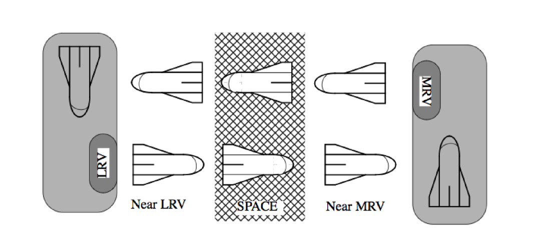
Figure 1: Space shuttle docking problem

Objective. The parity objective of the model is defined by the priority assignment function as follows: all states from 1 to 7 have priority $3$; the state 8 which represents a successful delivery into a least recently visited station, has priority $2$. Whenever the shuttle is facing a station, it should try to backup into the station as trying to move forward results into a bump into a station represented with states 9 and 10 with priority $1$. Therefore, the objective can be intuitively explained as trying to visit both of the stations infinitely often, while trying to bump only finitely often with probability $1$.

The input file for the POMDP can be downloaded here http://pub.ist.ac.at/pps/examples/Space_shuttle_small.txt. The more complex variants of this model differ in the number of states that are required to travel through the space, and therefore have higher uncertainty about the position of the shuttle.

B-B Example - Cheese Maze

The maze is shown in Figure 2 is introduced in [22]. We will describe only the smallest variant in detail. The goal of the player is to reach a goal state while trying to avoid poison in bad states. The player is only partially informed, its observation corresponds to what would be seen in all four directions immediately adjacent to the location. After the goal state is reached the player is respawned with positive probability in multiple states of the maze and the game is restarted.

States: There are $11$ states in the POMDP that are illustrated on Figure 2. The game starts in state 6. The poison is placed in states 8 and 9, and 10 is the goal state.

Observations: There are $7$ observations corresponding to what would be seen in all four directions immediately adjacent to the location, i.e., states 5, 6, and 7 do have the same observation. The observations are as follows: o0, the walls are NW; o1, the walls are NS; o2, the wall is N; o3, the walls are NE; o4, the walls are WE; o5, a poisoned state; and o6, the goal state.

Actions: There are four actions available corresponding to the movement in the four compass directions (north n, east e, south s, west w).

Transition relation: Actions that attempt to move outside of the maze have no effect on the position. The rest of the moves is deterministic in all $4$ actions.

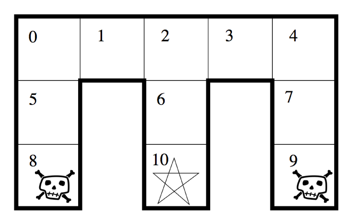
Figure 2: Cheese maze problem

Objective: The objective is to visit the goal state 10 infinitely often, while getting poisoned in states 8 and 9 only finitely often. This is encoded as a parity objective with 3 priorities. State 10 has priority 2, states 8 and 9 have priority 1, and every other state has priority 3. Whenever the goal state is reached, the maze is restarted with probability $1/3$ to state 0, with probability $1/3$ to state 2, and with probability $1/3$ to state 4 in the easiest variant of the problem.

The other variants are medium and difficult, and differ in the number of states the maze can restart to, intuitively increasing the uncertainty in the POMDP and also result into longer running times. We also consider a more difficult setting of the problem by constructing an intermediate and large size mazes with more states but based on the same principle. The input file for the POMDP can be downloaded here http://pub.ist.ac.at/pps/examples/Small_cheese_maze_easy.txt.

B-C Example - Grid

We will describe only the grid $4\times 4$, the other larger variants of the grid only differ in size. The problem consists of a $4$ by $4$ grid of locations. There is a single goal state, and multiple trap states that are placed beforehand but not known to the player. Whenever a goal state is reached the game is restarted. The goal of the player is to learn the position of the traps and visit the goal infinitely often, while visiting the trap state only finitely often with probability $1$.

States: There are $33$ states in the POMDP. The uncertainty about the placement of the traps is modeled by two grids of states $4\times 4$ and an additional initial state start that has transition to both of the grids. The coding of the states is as follows, the state ijk corresponds to a state in the $i$-th copy, $j$-th row, and $k$-th column. The goal state in each grid is the lower right corner, i.e., state 033 and 133 (rows and columns are numbered $0$-$3$).

Figure 3: Trap placement

Observations: There are $4$ observations, the initial state has observation o0, the trap states have observation o2, the goal state has observation o3, and all the remaining states have observation o1.

Actions: As in the previous example, there are $4$ actions available corresponding to the movement in the four compass directions (north n, east e, south s, west w).

Transition relation: The initial state of the POMDP is the state start, no matter what action is played the next state is with probability $0.5$ the upper left corner in one of the grids, and with the remaining probability the upper left corner of the second grid. In the grid all the actions are deterministic and attempts to move outside of the grid have no effect on the position. Whenever a goal state is reached the game is restarted the the upper left corner of the same grid (the trap states stay in the same position).

Objective: The objective is to learn in which grids the player is and as in the previous examples try to reach the goal state infinitely often while visiting the trap states only finitely often with probability $1$. This is encoded as a parity objective with $3$ priorities, the goal state has priority $2$, the trap states have priority $1$, and all the remaining states have priority $3$.

The placement of the trap states we have considered for the $4\times 4$ grid is depicted on Figure 3. The other variants differ in the size of the grid and placements of the trap states. The input file for the POMDP can be downloaded here http://pub.ist.ac.at/pps/examples/4x4_grid.txt.

B-D RockSample problems.

We consider a modification of the RockSample problem introduced in [29] and used later in [3]. It is a scalable problem that models rover science exploration. The rover is equipped with a limited amount of fuel and can increase the amount of fuel by sampling rocks in the immediate area. The positions of the rover and the rocks are known, but only some of the rocks can increase the amount of fuel; we will call these rocks good. The type of the rock is not known to the rover, until the rock is sampled. Once a good rock is used to increase the amount of fuel, it becomes temporarily a bad rock until all other good rocks are sampled. We consider variants with different maximum capacity of the rover’s fuel tank. An instance of the RockSample problem is parametrized with two parameters $[n,k]$: map size $n\times n$ and $k$ rocks is described as RockSample[n,k]. The POMDP model of RockSample[n,k] is as follows:

States: The state space is the cross product of $2k+1+c$ features: $\mathit{Position}=\{(1,1),(1,2),...,(n,n)\}$, $2*k$ binary features $\mathit{RockType}_{i}=\{\mathit{Good},\mathit{Bad}\}$ that indicate which of the rocks are good and which rocks are temporarily not able to increase the amount of fuel, and $c$ is the amount of fuel remaining in the fuel tank.

Observations: There are four observations: the unique observation for the initial state, two observations to denote whether the rock that is sampled is good or bad. The last observation is for all the remaining states.

Actions: The rover can select four actions: $\{N,S,E,W\}$.

Transition relation: All the actions are deterministic single-step motion actions. A rock is sampled whenever the rock is at the rover’s current location.

Objective: If the rock is good, the fuel amount is increased to the maximum capacity and the rock becomes temporarily bad. Every state of the POMDP has priority $2$ with the following two exceptions:

• In a state where the rover samples a bad rock (also temporarily bad rocks) the priority $1$.

• In a state where the fuel amount decreases to $0$ the priority is also 1.

The instance RS[4,2] (resp. RS[4,3]) is depicted on Figure 5 (resp. Figure 5), the arrow indicates the initial position of the rover and the filled rectangles denote the fixed positions of the rocks. A variant of the input file for the POMDP can be downloaded here http://pub.ist.ac.at/pps/examples/RS4_2_3.txt.

Figure 4: RS[4,2]

Figure 5: RS[4,3]

B-E Hallway problems.

We consider two versions of the Hallway problems introduced in [22] and used later in [31, 29, 3]. The basic idea behind both of the Hallway problems, is that there is an agent wandering around an office building. It is assumed that the locations have been discretized so there are a finite number of locations where the agent could be. The agent has a small finite set of actions it can take, but these only succeed with some probability. In these problems the location in the building and the agent’s current orientation comprise the states. The smaller Hallway POMDP is depicted in Figure LABEL:fig:hallway1 and the larger Hallway POMDP is depicted in Figure LABEL:fig:hallway2. We will describe the smaller problem Hallway in more detail:

Figure 6: Hallway POMDP

States: There are $15$ locations in the office times the four possible orientations together with an auxiliary starting and loosing state is $62$. All the objectives are expressed as deterministic parity automata. The final size of the POMDP $62$ multiplied by the number of states of the parity automaton.

Observations: the agent is equipped with very short range sensors to provide it only with information about whether it is adjacent to a wall. The sensors can ”see” in four directions: forward, left, right, and backward. It is important to note that these observations are relative to the current orientation of the agent (N, E, S, W).

Figure 7: Hallway 2 POMDP

Actions: There are three actions that can be chosen: forward, turn-left, and turn-right.

Transition relation: The agent starts with uniform probability in the states labeled with the + symbol in any of the four possible orientations. The actions that can be chosen consists of movements: forward, turn-left, and turn-right. All the available actions succeed with probability $0.8$ and with probability $0.2$ the state is not changed. In states where moving forward is impossible the probability mass for the impossible next state is collapsed into the probability of not changing the state.

Objective: There are four dedicated areas in the office, denoted by letters A,B,C, and D. We consider four objectives in both the Hallway problems:

• Liveness: requires that the $D$-labeled state is reached. The automaton consists of $2$ states.

• Sequencing and avoiding obstacles: requires that first the $A$-labeled state is visited, followed by the $B$-labeled state and finally the $D$-labeled state is visited while avoiding the $C$-labeled state. The automaton consists of $5$ states.

• Coverage: requires that the $A$, $B$, and $C$-labeled states are all visited in any order. The automaton consists of $8$ states.

• Recurrence: requires that both the $A$ and $C$-labeled states are visited infinitely often. The automaton consists of $4$ states.

• Recurrence and avoidance: requires that both $A$ and $D$-labeled states are visited infinitely often, while visiting $B$ and $C$-labeled states only finitely many times. The automaton consists of $5$ states.

A variant of the input file of the POMDP can be downloaded here http://pub.ist.ac.at/pps/examples/hallwayLiv.txt.

B-F Maze navigation problems.

We consider three variants of the mazes introduced in [14]. Intuitively, the robot navigates itself in a grid discretization of a 2D world. The robot can choose from four noise free actions north, east, south, and west. In every maze there are $4$ highlighted regions that are labeled with letters $A$, $B$, $C$, and $D$. The objective for the robot is given as a deterministic parity automaton, as in the case of Hallway problems. We describe fully Maze A, the other problems differ only in the structure of the maze:

Figure 8: POMDP Maze A

Figure 9: POMDP Maze B

States: The state space of Maze A consists of $84$ possible grid locations times the number of states of the parity automaton that defines the objective. The robot moves from the unique initial states uniformly at random under all actions in all the locations labeled with ”+”.

Observations: The highlighted regions are observable to the robot, otherwise the robot does not receive any feedback from the maze.

Actions: There are four actions that can be chosen: $\{N,S,E,W\}$.

Transition relation: All the available actions succeed with probability $1$. In states where robot attempts to move outside of the maze or in the wall the position of the robot remains unchanged.

Figure 10: POMDP Maze C

Objective: We consider the same objectives as in the case of the Hallway problems:

• Liveness: requires that the $D$-labeled state is reached. The automaton consists of $2$ states.

• Sequencing and avoiding obstacles: requires that first the $A$-labeled state is visited, followed by the $B$-labeled state and finally the $D$-labeled state is visited while avoiding the $C$-labeled state. The automaton consists of $5$ states.

• Coverage: requires that the $A$, $B$, and $C$-labeled states are all visited in any order. The automaton consists of $8$ states.

• Recurrence: requires that both the $A$ and $C$-labeled states are visited infinitely often. The automaton consists of $4$ states.

• Recurrence and avoidance: requires that both $A$ and $D$-labeled states are visited infinitely often, while visiting $B$ and $C$-labeled states only finitely many times. The automaton consists of $5$ states.

A variant of the input file of the POMDP can be downloaded here http://pub.ist.ac.at/pps/examples/mazeALiv.txt.

References

- [1] M. Antoniotti and B. Mishra. Discrete event models + temporal logic = supervisory controller: Automatic synthesis of locomotion controllers. In ICRA. IEEE, 1995.
- [2] C. Baier, M. Größer, and N. Bertrand. Probabilistic omega-automata. J. ACM, 59(1), 2012.
- [3] B. Bonet and H. Geffner. Solving POMDPs: RTDP-Bel vs. point-based algorithms. In IJCAI, 2009.
- [4] K. Chatterjee, M. Chmelik, and M. Tracol. What is Decidable about Partially Observable Markov Decision Processes with omega-Regular Objectives. In CSL, 2013.
- [5] K. Chatterjee, M. Henzinger, M. Joglekar, and N. Shah. Symbolic algorithms for qualitative analysis of Markov decision processes with Büchi objectives. FMSD, 2013.
- [6] Y. Chen, J. Tumová, and C. Belta. LTL robot motion control based on automata learning of environmental dynamics. In ICRA. IEEE, 2012.
- [7] L. Chrisman. Reinforcement learning with perceptual aliasing: The perceptual distinctions approach. In AAAI. Citeseer, 1992.
- [8] I. Cizelj and C. Belta. Control of noisy differential-drive vehicles from time-bounded temporal logic specifications. In ICRA, 2013.
- [9] E.M. Clarke, O. Grumberg, and D. Peled. Model checking. MIT press, 1999.
- [10] G.E. Fainekos, H. Kress-Gazit, and G.J. Pappas. Hybrid controllers for path planning: A temporal logic approach. In CDC-ECC. IEEE, 2005.
- [11] G.E. Fainekos, H. Kress-Gazit, and G.J. Pappas. Temporal logic motion planning for mobile robots. In ICRA. IEEE, 2005.
- [12] J. Filar and K. Vrieze. Competitive Markov Decision Processes. Springer-Verlag, 1997.
- [13] J. Fu, R. Dimitrova, and U. Topcu. Abstractions and sensor design in partial-information, reactive controller synthesis. In American Control Conference (ACC), pages 2297–2304. IEEE, 2014.
- [14] D. Grady, M. Moll, and L.E. Kavraki. Automated Model Approximation for Robotic Navigation with POMDPs. In ICRA. IEEE, 2013.
- [15] M. Guo, K.H. Johansson, and D.V. Dimarogonas. Revising motion planning under linear temporal logic specifications in partially known workspaces. In ICRA, 2013.
- [16] T.A. Henzinger, P.H. Ho, and H. Wong-Toi. HyTech: A model checker for hybrid systems. In CAV. Springer, 1997.
- [17] H. Howard. Dynamic Programming and Markov Processes. MIT Press, 1960.
- [18] K. Hsiao, L.P. Kaelbling, and T. Lozano-Perez. Grasping POMDPs. In ICRA. IEEE, 2007.
- [19] L. P. Kaelbling, M. L. Littman, and A. R. Cassandra. Planning and acting in partially observable stochastic domains. AI, 1998.
- [20] H. Kress-Gazit, G. E. Fainekos, and G. J. Pappas. Temporal-logic-based reactive mission and motion planning. IEEE Transactions on Robotics, 2009.
- [21] H. Kurniawati, D. Hsu, and W.S. Lee. SARSOP: Efficient point-based POMDP planning by approximating optimally reachable belief spaces. In Robotics: Science and Systems, 2008.
- [22] M. L. Littman, A. R. Cassandra, and L. P. Kaelbling. Learning policies for partially observable environments: Scaling up. In ICML. Citeseer, 1995.
- [23] C. H. Papadimitriou and J. N. Tsitsiklis. The complexity of Markov decision processes. Mathematics of Operations Research, 1987.
- [24] A. Paz. Introduction to probabilistic automata. Academic Press, 1971.
- [25] N. Piterman. From nondeterministic Buchi and Streett automata to deterministic parity automata. In LICS. IEEE, 2006.
- [26] V. Raman, N. Piterman, and H. Kress-Gazit. Provably correct continuous control for high-level robot behaviors with actions of arbitrary execution durations. In ICRA, 2013.
- [27] N. Roy, W. Burgard, D. Fox, and S. Thrun. Coastal navigation-mobile robot navigation with uncertainty in dynamic environments. In ICRA. IEEE, 1999.
- [28] Shmuel Safra. On the complexity of -automata. In FOCS. IEEE, 1988.
- [29] T. Smith and R. Simmons. Heuristic search value iteration for POMDPs. In UAI. AUAI Press, 2004.
- [30] T. Smith and R. Simmons. Point-Based POMDP Algorithms: Improved Analysis and Implementation. In UAI. AUAI Press, 2005.
- [31] M.T.J. Spaan. A point-based POMDP algorithm for robot planning. In ICRA. IEEE, 2004.
- [32] S. Thrun, W. Burgard, and D. Fox. Probabilistic robotics. MIT Press, 2005.
- [33] M. Y. Vardi. Automatic verification of probabilistic concurrent finite-state systems. In FOCS. IEEE, 1985.