Periodic orbit analysis for the deterministic path-preference traffic flow cellular automaton

Yoichi Nakata ynakata@ms.u-tokyo.ac.jp Isotope Science Center, the University of Tokyo, 2-11-16 Yayoi, Bunkyo-ku, Tokyo 113-0032, Japan    Yoshihiro Ohta Institute of Biology and Mathematics (iBMath), Interdisciplinary Center of Mathematical Sciences, Graduate School of Mathematical Sciences, the University of Tokyo, 3-8-1 Komaba, Meguro-ku, Tokyo 153-8914, Japan    Sigeo Ihara Institute of Biology and Mathematics (iBMath), Interdisciplinary Center of Mathematical Sciences, Graduate School of Mathematical Sciences, the University of Tokyo, 3-8-1 Komaba, Meguro-ku, Tokyo 153-8914, Japan Research Center for Advanced Science and Technology, the University of Tokyo, 4-6-1 Komaba, Meguro-ku, Tokyo 153-8904, Japan
Abstract

The path-preference traffic flow cellular automaton is suggested to model the dynamics of transcription. The main difference from the simple traffic flow model is that it contains another preferential paths at some sites. In this paper, we propose an exact analysis for the simplest version of this model. We find that the number of particles is dominant to the dynamics of this cellular automaton and observed that there are not only expected phase shift but also several gaps as the number of particles increases. By considering the behavior of periodic orbits, we also determine the point where such gaps in the flow appear and the exact value of the flow.

Cellular Automaton, Traffic Jams
pacs:
89.40.-a, 45.70.Vn, 05.45.-a, 47.54.-r, 87.16.A-, 87.15.hj, 47.63.-b

I Introduction

Discrete dynamical systems with discrete dependent variables are called cellular automata. They contain very rich structures and are applied to various area even if they have simple time evolution rules. Elementary Cellular Automaton (ECA) is one of good examples. This system consists on a sequence of sites and each site can take only two values and the time evolution of a site is defined only by the nearest neighbor sites Wolfram . However, the ECA forms interesting time-space patterns and similar dynamics appears in various fields (for instance BelitskyFerrari ).

The asymmetric simple exclusive process (ASEP) is a stochastic cellular automaton on one dimensional and originally presented as a model representing the dynamics of ribosomes in translation on RNA MacDonaldGibbsPipkin , which is currently famous as the cellular automaton model representing the dynamics of traffic flow Derrida . The model restricting the direction of the movement in the ASEP is called the TASEP and the deterministic version of the TASEP is the ECA rule 184, which is directly related to the differential equation expressing car traffics through the limiting procedure called “ultradiscretization” TokihiroTakahashiMatsukidairaSatsuma .

It is known that several phases exist in the states of the TASEP after a sufficient time has passed and such phases depend on the parameters of the system. In that of the ECA 184, there are two phases where particles move freely or make a traffic jam and it is known that the density of particles determines the phases SchadschneiderSchreckenberg .

The path-preference cellular automaton model proposed by one of the authors and Nishiyama et al. should be interpreted as a model introducing a shortcut (or branching and jointing) for the TASEP and to explain the behavior of RNA Polymerase II in the transcription dynamics of eucaryotes OhtaNishiyama . Shortcuts mean that RNAPII will skip over the tracks that should be inherently due to the spatial proximity of the DNA placed in the high dimensional space and diffusion effect. Regulating the expression of function by the spatial structure of DNA has been actively studied particularly in recent yearsCook ; PapantonisLarkinWadaOhtaIharaKodamaCook ; FraserBickmore . On the other hand, to express transcription dynamics, several cellular automata model of RNAPII dynamics have been presented OhtaKodamaIhara ; TripathiChowdhury ; TripathiSchutzChowdhury . Therefore, this model is a cellular automaton model to describe the dynamics of RNAPII in the three dimensional space. In this paper, we deal with a deterministic version of this model (i.e. an extension of ECA 184).

The existence of such shortcuts make the behavior of the system even more complicated and interesting. Numerical simulation confirms that discontinuous change in flow rate occurs by changing the number of particles, which is a major difference from the behavior of the ECA 184 BrankovPeshevaBunzarova ; Negami . Our target is to reveal the reason of such a phenomenon.

In this paper, we focus on periodic orbits of this system. For such periodic orbits, the flow rate can be computed exactly and we confirmed that it agrees with the numerical simulation. Furthermore, we find that the discontinuous change in the flow rate is due to transition to another class of periodic orbits by breaking the condition where the periodic orbit should hold.

Different from the ECA 184, orbits are found to be possibly attracted by different types of periodic orbits for some configurations even when the number of particles is the same. Although these orbits are unstable by the perturbations such as slightly altering the configuration of the particles, we have constructed a method to construct the trajectory. Furthermore, we have calculated the values such as the flow rate and the period of the orbit and discussed the conditions where such periodic orbits hold.

Conventionally, analysis using a statistical physics model has been actively performed for such a model TannaiNishinari . We however propose the analysis by focusing on the orbit itself. In the analysis, we focus on the specific pattern through which orbits must pass, which is considered as an analogue of the Poincaré section in the dynamical system theory.

II Path-preference cellular automaton model

II.1 Modeling

We first define the model which we deal with. This model is a special case of the path-preference cellular automaton model OhtaNishiyama .

The model is an extension of the ECA Rule 184. That is, basically the system consists of a finite amount of the sequence of boxes and a finite amount of balls and a box can contain at most one ball. A ball moves to the next box if there are no other balls. One time step evolution of this system is done when all ball move or stay. The destination of the ball at the last site is the first one, which means the periodic boundary condition. We denote the number of boxes and balls as N𝑁N and M𝑀M, respectively and assign the number for each box in a sequential order. However, at some sites the balls can also jump to the remote sites, not only the next sites. We denote ϵksubscriptitalic-ϵ𝑘\epsilon_{k} as the site number of such a site and ιksubscript𝜄𝑘\iota_{k} as that of jump destination sites from ϵksubscriptitalic-ϵ𝑘\epsilon_{k}-th site. We also assume that ϵksubscriptitalic-ϵ𝑘\epsilon_{k} and ιksubscript𝜄𝑘\iota_{k} have the relation:

1ιK<ϵ1<<ι1<ϵ2<<ι2<<ϵK<<N,1subscript𝜄𝐾subscriptitalic-ϵ1much-less-thansubscript𝜄1subscriptitalic-ϵ2much-less-thansubscript𝜄2subscriptitalic-ϵ𝐾much-less-than𝑁1\leq\iota_{K}<\epsilon_{1}<<\iota_{1}<\epsilon_{2}<<\iota_{2}<\ldots<\epsilon_{K}<<N,

where x<<ymuch-less-than𝑥𝑦x<<y means yx2𝑦𝑥2y-x\geq 2. We can set ιK=1subscript𝜄𝐾1\iota_{K}=1 without loss of generality because of the periodic boundary condition.

By setting these bifurcations, there are possibilities such that a ball can go to several destination and several balls are going to the same site at some time. For such cases, we introduce the following rules:

  • The ball at ϵksubscriptitalic-ϵ𝑘\epsilon_{k}-th box jumps to ιksubscript𝜄𝑘\iota_{k}-th one when there are no balls at ιksubscript𝜄𝑘\iota_{k}-th (even if there is a ball at ιk1subscript𝜄𝑘1\iota_{k}-1-th).

  • The ball at (ιk1)subscript𝜄𝑘1(\iota_{k}-1)-th box moves to ιksubscript𝜄𝑘\iota_{k}-th one only when there are no balls at ιksubscript𝜄𝑘\iota_{k}-th and ϵksubscriptitalic-ϵ𝑘\epsilon_{k}-th.

Refer to caption
Figure 1: The ball at ϵksubscriptitalic-ϵ𝑘\epsilon_{k}-th site jumps to ιksubscript𝜄𝑘\iota_{k}-th site if there are no balls and the ball at (ιk1)subscript𝜄𝑘1(\iota_{k}-1)-th box cannot move to the next if a ball jumps to there.
Refer to caption
Figure 2: The ball at ϵksubscriptitalic-ϵ𝑘\epsilon_{k}-th site jumps to the next if there is a ball at ιksubscript𝜄𝑘\iota_{k}-th and there are no balls at the next site.

This rule indicates that we set a priority for balls jumping via shortcut. We call this rule “jump priority”. Inversely, we can also set the priority for balls moving to next sites. We call this rule “move priority”. In this paper, we employ jump priority just because of the mathematical symmetry described as follows but not to reflect the real dynamics which the original model tends to represent.

With the definitions above, let us introduce the mathematical expression of the time evolution rule of this system. We set ujtsubscriptsuperscript𝑢𝑡𝑗u^{t}_{j} the number of balls (which takes 00 or 111) at the j𝑗j-th site in time t𝑡t and f(k,l)𝑓𝑘𝑙f(k,l) the number of transiting balls from k𝑘k-th site to l𝑙l-th. Hereafter, we use the letter j𝑗j for indicating the site number. Due to the time evolution rule, the movement of a ball to the next site is expressed as

f(j,j+1)=min(ujt,1uj+1t)𝑓𝑗𝑗1subscriptsuperscript𝑢𝑡𝑗1subscriptsuperscript𝑢𝑡𝑗1f(j,j+1)=\min(u^{t}_{j},1-u^{t}_{j+1}) (1)

for jϵk𝑗subscriptitalic-ϵ𝑘j\neq\epsilon_{k} (k=1,2,,K𝑘12𝐾k=1,2,\ldots,K).

Since we introduce the jump priority rule, the number of jumping balls from ϵksubscriptitalic-ϵ𝑘\epsilon_{k}-th to ιksubscript𝜄𝑘\iota_{k}-th is

f(ϵk,ιk)=min(uϵkt,1uιkt).𝑓subscriptitalic-ϵ𝑘subscript𝜄𝑘subscriptsuperscript𝑢𝑡subscriptitalic-ϵ𝑘1subscriptsuperscript𝑢𝑡subscript𝜄𝑘f(\epsilon_{k},\iota_{k})=\min(u^{t}_{\epsilon_{k}},1-u^{t}_{\iota_{k}}). (2)

In the case f(ϵk,ιk)=1𝑓subscriptitalic-ϵ𝑘subscript𝜄𝑘1f(\epsilon_{k},\iota_{k})=1, those of moving balls are written in

f(ϵk,ϵk+1)=0𝑓subscriptitalic-ϵ𝑘subscriptitalic-ϵ𝑘10\displaystyle f(\epsilon_{k},\epsilon_{k}+1)=0 (3)
f(ιk1,ιk)=0𝑓subscript𝜄𝑘1subscript𝜄𝑘0\displaystyle f(\iota_{k}-1,\iota_{k})=0 (4)

and in the case f(ϵk,ιk)=0𝑓subscriptitalic-ϵ𝑘subscript𝜄𝑘0f(\epsilon_{k},\iota_{k})=0,

f(ϵk,ϵk)=min(uϵkt,1uϵk+1t)𝑓subscriptitalic-ϵ𝑘subscriptitalic-ϵ𝑘subscriptsuperscript𝑢𝑡subscriptitalic-ϵ𝑘1subscriptsuperscript𝑢𝑡subscriptitalic-ϵ𝑘1\displaystyle f(\epsilon_{k},\epsilon_{k})=\min(u^{t}_{\epsilon_{k}},1-u^{t}_{\epsilon_{k}+1}) (5)
f(ιk1,ιk)=min(uιk1t,1uιkt).𝑓subscript𝜄𝑘1subscript𝜄𝑘subscriptsuperscript𝑢𝑡subscript𝜄𝑘11subscriptsuperscript𝑢𝑡subscript𝜄𝑘\displaystyle f(\iota_{k}-1,\iota_{k})=\min(u^{t}_{\iota_{k}-1},1-u^{t}_{\iota_{k}}). (6)

Here, we consider the modulo of N𝑁N for the index of the site number.

Then, we obtain the time evolution rule:

uϵkt+1=uϵkt+f(ϵk1,ϵk)f(ϵk,ιk+1)f(ϵk,ϵk+1)subscriptsuperscript𝑢𝑡1subscriptitalic-ϵ𝑘subscriptsuperscript𝑢𝑡subscriptitalic-ϵ𝑘𝑓subscriptitalic-ϵ𝑘1subscriptitalic-ϵ𝑘𝑓subscriptitalic-ϵ𝑘subscript𝜄𝑘1𝑓subscriptitalic-ϵ𝑘subscriptitalic-ϵ𝑘1\displaystyle u^{t+1}_{\epsilon_{k}}=u^{t}_{\epsilon_{k}}+f(\epsilon_{k}-1,\epsilon_{k})-f(\epsilon_{k},\iota_{k}+1)-f(\epsilon_{k},\epsilon_{k}+1) (7)
uιkt+1=uιkt+f(ιk1,ιk)+f(ϵk,ιk)f(ιk,ιk+1)subscriptsuperscript𝑢𝑡1subscript𝜄𝑘subscriptsuperscript𝑢𝑡subscript𝜄𝑘𝑓subscript𝜄𝑘1subscript𝜄𝑘𝑓subscriptitalic-ϵ𝑘subscript𝜄𝑘𝑓subscript𝜄𝑘subscript𝜄𝑘1\displaystyle u^{t+1}_{\iota_{k}}=u^{t}_{\iota_{k}}+f(\iota_{k}-1,\iota_{k})+f(\epsilon_{k},\iota_{k})-f(\iota_{k},\iota_{k}+1) (8)

for k=1,,K𝑘1𝐾k=1,\ldots,K and

ujt+1=ujt+f(j1,j)f(j,j+1).subscriptsuperscript𝑢𝑡1𝑗subscriptsuperscript𝑢𝑡𝑗𝑓𝑗1𝑗𝑓𝑗𝑗1u^{t+1}_{j}=u^{t}_{j}+f(j-1,j)-f(j,j+1). (9)

for other sites.

By adding this formula for j=1,,N𝑗1𝑁j=1,\ldots,N, one has j=1Nujt+1=j=1Nujtsuperscriptsubscript𝑗1𝑁subscriptsuperscript𝑢𝑡1𝑗superscriptsubscript𝑗1𝑁subscriptsuperscript𝑢𝑡𝑗\sum_{j=1}^{N}u^{t+1}_{j}=\sum_{j=1}^{N}u^{t}_{j}, which means the conservation law of the total number of balls. Furthermore, when introducing a new dependent variable vjt:=1ujtassignsubscriptsuperscript𝑣𝑡𝑗1subscriptsuperscript𝑢𝑡𝑗v^{t}_{j}:=1-u^{t}_{j}, the time evolution rule of vjtsubscriptsuperscript𝑣𝑡𝑗v^{t}_{j} is the same as that of ujtsubscriptsuperscript𝑢𝑡𝑗u^{t}_{j} under the replacement jj𝑗𝑗j\to-j, which means that the dynamics is the same under the inverted direction when interchanging empty sites and occupied ones. Such a good symmetry does not hold if one sets the move priority rule.

Since this model is deterministic and the states are finite amount, an orbit which starts from an arbitrary initial state is finally attracted by a periodic orbit (the steady states are regarded as the periodic orbits with period 1), which should be called as the limit cycle.

III Analysis of the simplest case: K=1𝐾1K=1

We first consider the simplest case K=1𝐾1K=1. In this case, the site where a ball can shortcut is only j=ϵ1𝑗subscriptitalic-ϵ1j=\epsilon_{1} and the destination site is j=ι1=1𝑗subscript𝜄11j=\iota_{1}=1. We call the sites from j=1𝑗1j=1 to j=ϵ1𝑗subscriptitalic-ϵ1j=\epsilon_{1} the main region and those from j=ϵ1+1𝑗subscriptitalic-ϵ11j=\epsilon_{1}+1 to j=N𝑗𝑁j=N the skipped region. We also define Nmsubscript𝑁𝑚N_{m} and Nssubscript𝑁𝑠N_{s} as the length of the main region and that of the skipped region, respectively.

III.1 Aspect of the system

We first consider the behavior of this system by focusing on the number of balls M𝑀M. In the case that M𝑀M are sufficiently small, all balls are finally trapped by the main region once they arrived there for most of initial values (See Fig. 3). Such behavior can be kept while MNm/2𝑀subscript𝑁𝑚2M\leq N_{m}/2. If M>Nm/2𝑀subscript𝑁𝑚2M>N_{m}/2, the main region cannot hold all balls and overflowed ones are emitted to the skipped region. In other words, the traffic on the main region is always optimized for maximizing its flow efficiency. In particular, if Nmsubscript𝑁𝑚N_{m} is even, balls in the main region generate a closed flow which prohibits other balls to join and those in the skipped region never come back to the main region and finally cause the unsolvable traffic jam at the end of the skipped region. If Nmsubscript𝑁𝑚N_{m} is odd, there is at least one area which satisfies ujt=0subscriptsuperscript𝑢𝑡𝑗0u^{t}_{j}=0 and uj+1t=0subscriptsuperscript𝑢𝑡𝑗10u^{t}_{j+1}=0 in the main region for any limit cycles. At space-time pattern, this area looks like a notch, which permits the balls at the skipped region to move back to the main region and helps the dynamics be richer. In this paper, we mainly consider the case Nmsubscript𝑁𝑚N_{m} is odd.

Refer to caption
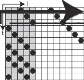
Figure 3: An example of general orbits for Nm=5subscript𝑁𝑚5N_{m}=5, Ns=8subscript𝑁𝑠8N_{s}=8, M=2𝑀2M=2. The sites of the main region are gray-meshed.

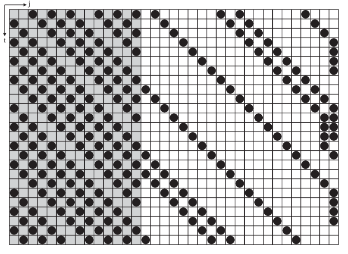
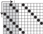
The limit cycles starting from most of the initial states have certain behaviors determined by the number of balls M𝑀M. However, some limit cycles starting from some special initial states show behaviors out from them. For example, in the time space pattern in Fig. 4, one ball is not trapped by the main region and goes around the skipped region even if the system satisfies MNm/2𝑀subscript𝑁𝑚2M\leq N_{m}/2. Such orbits occur because the configurations are well balanced and are easily attracted by other orbits with a little perturbation such as shifting one of balls to the neighbor empty site. We call these unstable orbits “special periodic orbits” and we call the orbits which are started from most of initial states and robust for little perturbation as “general periodic orbits”.
Refer to caption
Figure 4: An example of special periodic orbits. The system parameters are the same as those in Fig. 3.

III.2 Analysis focusing on flow

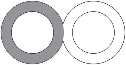
The value “flow”, which is defined as the number of moving balls per a site, is a powerful tool for analyzing the behavior of the general traffic models. However, it is not naively applicable for this model because there is an ambiguity of the distance for the jump. If one wants to match a model with experiments, we should take this distance properly. For example, it should be 111 for the figure of 8-shape form like Fig. 5 and it is taken as the length of the hurdled intron in the original path-preference model. In this paper, we consider the flow of each region instead of the flow of whole the system to focus on mathematical properties. We also ignore the movement between two regions. Then, we define Jmsubscript𝐽𝑚J_{m} and Jssubscript𝐽𝑠J_{s} as the flow of the main region and the skipped one respectively, which are written in

Jm=Jm(t):=1Nm1j=1Nm1f(j,j+1)subscript𝐽𝑚subscript𝐽𝑚𝑡assign1subscript𝑁𝑚1superscriptsubscript𝑗1subscript𝑁𝑚1𝑓𝑗𝑗1\displaystyle J_{m}=J_{m}(t):=\frac{1}{N_{m}-1}\sum_{j=1}^{N_{m}-1}f(j,j+1) (10)
Js=Js(t):=1Ns1j=Nm+1N1f(j,j+1).subscript𝐽𝑠subscript𝐽𝑠𝑡assign1subscript𝑁𝑠1superscriptsubscript𝑗subscript𝑁𝑚1𝑁1𝑓𝑗𝑗1\displaystyle J_{s}=J_{s}(t):=\frac{1}{N_{s}-1}\sum_{j=N_{m}+1}^{N-1}f(j,j+1). (11)

We also define the time average of value X𝑋X(=Jm,Jsabsentsubscript𝐽𝑚subscript𝐽𝑠=J_{m},J_{s}) by

X=limT1Tt=0T1X(t).delimited-⟨⟩𝑋subscript𝑇1𝑇superscriptsubscript𝑡0𝑇1𝑋𝑡\displaystyle\langle X\rangle=\lim_{T\to\infty}\frac{1}{T}\sum_{t=0}^{T-1}X(t). (12)

Now, remember that arbitrary orbit is attracted by a periodic orbit. By defining the period of the orbit as T𝑇T, one can rewrite

X=1Tt=t0t0+T1X(t)delimited-⟨⟩𝑋1𝑇superscriptsubscript𝑡subscript𝑡0subscript𝑡0𝑇1𝑋𝑡\displaystyle\langle X\rangle=\frac{1}{T}\sum_{t=t_{0}}^{t_{0}+T-1}X(t) (13)

for sufficiently large t0subscript𝑡0t_{0}. We note that the period depends of the initial states, i.e. T=T({uj0}j=1N)𝑇𝑇superscriptsubscriptsubscriptsuperscript𝑢0𝑗𝑗1𝑁T=T(\{u^{0}_{j}\}_{j=1}^{N}).

Refer to caption
Figure 5: An expression of one main and skipped regions model.
Refer to caption
Figure 6: The graph of the flow in the main region Jmdelimited-⟨⟩subscript𝐽𝑚\langle J_{m}\rangle for several initial state for each M𝑀M where Nm=301subscript𝑁𝑚301N_{m}=301 and Ns=700subscript𝑁𝑠700N_{s}=700.
Refer to caption
Figure 7: The graph of the flow in the skipped region Jsdelimited-⟨⟩subscript𝐽𝑠\langle J_{s}\rangle for several initial state for each M𝑀M where Nm=301subscript𝑁𝑚301N_{m}=301 and Ns=700subscript𝑁𝑠700N_{s}=700.

FIG. 7 and 7 are graphs relating between the flow Jmdelimited-⟨⟩subscript𝐽𝑚\langle J_{m}\rangle, Jsdelimited-⟨⟩subscript𝐽𝑠\langle J_{s}\rangle and the number of balls M𝑀M for fixed Nmsubscript𝑁𝑚N_{m} and Nssubscript𝑁𝑠N_{s} (we consider several initial states for each M𝑀M). One can find that not only phase shift around M=Nm/2𝑀subscript𝑁𝑚2M=N_{m}/2 discussed above but also several non-continuous gaps appear in the flow in the skipped region. One can also observe that the flow in the skipped region can take several value for some M𝑀M. We note that the graph is symmetric with M=N/2𝑀𝑁2M=N/2 because of the symmetry due to the jump priority time evolution rule. To discuss the reason of such phenomena including the exact point of gaps and the flow of each part, we focus on several representative periodic orbits.


III.3 Periodic orbit: class 1-0

We first consider the case where N𝑁N is even and M=N/2𝑀𝑁2M=N/2 (i.e. Nssubscript𝑁𝑠N_{s} is odd because we assume that Nmsubscript𝑁𝑚N_{m} is odd). In this case, arbitrary orbits are finally attracted by the limit cycle ujt=t+jsubscriptsuperscript𝑢𝑡𝑗𝑡𝑗u^{t}_{j}=t+j (mod 2mod2\mathrm{mod}\ 2) with period 222 and its time-space pattern forms a checkerboard one. The exact flow is

Jm=Js=12.delimited-⟨⟩subscript𝐽𝑚delimited-⟨⟩subscript𝐽𝑠12\langle J_{m}\rangle=\langle J_{s}\rangle=\frac{1}{2}. (14)

III.4 Periodic orbit: class 1-1

We next consider the case M<N/2𝑀𝑁2M<N/2, where the several sequential empty boxes appear in the limit cycles. We first focus attention on specific patterns in the skipped region of which one ball and one empty box appear alternately. We call such patterns “clusters”. Observation shows that there is a pair of sequential empty sites in the main region in most of time steps. We call such sites “notch”. The notch goes around in the main region.

The dynamics of periodic orbits are controlled by the number of clusters and the dynamics of the notch. We first consider the case that the limit cycle contains only one notch and one cluster.

We pay attention to the time when the notch is the top of the main region. We assume that the initial state is ujt=1subscriptsuperscript𝑢𝑡𝑗1u^{t}_{j}=1 (j=3,5,,2M3,2M1𝑗352𝑀32𝑀1j=3,5,\ldots,2M-3,2M-1) and ujt=0subscriptsuperscript𝑢𝑡𝑗0u^{t}_{j}=0 otherwise. The time when the head of the cluster arrives at the end is t0:=N2M1assignsubscript𝑡0𝑁2𝑀1t_{0}:=N-2M-1. While balls and empty boxes appears alternatively at the last site of the main region in time evolution, the balls in the skipped region can go back to the main region. Then, when the top of the cluster in the skipped region, it makes traffic jam until the notch arrives the last site of the main region. We define this time as t1:=Ne1assignsubscript𝑡1subscript𝑁𝑒1t_{1}:=N_{e}-1. In this case, one has the relation: t0t1subscript𝑡0subscript𝑡1t_{0}\leq t_{1}.

When the notch arrives there, the balls in the cluster go back to the main region. Next, when this ball arrives at the top of the main region, a ball is at the end of the main region and it cannot go to the top. Then, it is bumped out to the skipped region. In the next time, neither j=0𝑗0j=0 nor j=Ne𝑗subscript𝑁𝑒j=N_{e} is occupied. Then, a ball of the cluster goes back again. These processes repeated until all of the balls of the cluster go back to the main region. After all balls go back, there appears a new notch in the top and a ball in the end can go around in the main region again.

The number of emitted balls from the main region is the same as the number of balls existing in the skipped region for the initial state. Then, the state of the system when a new notch are created is nothing but the initial state. The time it takes for the balls making a jam to start going back to the main region and finish it is 2{M(Ne1)/2}2𝑀subscript𝑁𝑒122\{M-(N_{e}-1)/2\}. Therefore, the period of this orbit is T=t1+2{M(Ne1)/2}+1=2M+1𝑇subscript𝑡12𝑀subscript𝑁𝑒1212𝑀1T=t_{1}+2\{M-(N_{e}-1)/2\}+1=2M+1.

Now, the number of balls emitted to the skipped region per a period Q𝑄Q is the same as that in the skipped region at the initial state and written in

Q=MNe12.𝑄𝑀subscript𝑁𝑒12Q=M-\frac{N_{e}-1}{2}. (15)

The balls in the skipped region goes around this region just one time per a period. Then, the sum of the flow for whole the skipped region and a period is expressed as:

t=t0t0+T1j=Nm+1N1f(j,j+1)=Q(Ns1).superscriptsubscript𝑡subscript𝑡0subscript𝑡0𝑇1superscriptsubscript𝑗subscript𝑁𝑚1𝑁1𝑓𝑗𝑗1𝑄subscript𝑁𝑠1\sum_{t=t_{0}}^{t_{0}+T-1}\sum_{j=N_{m}+1}^{N-1}f(j,j+1)=Q(N_{s}-1). (16)

Then, the time average of the flow at the skipped region is expressed as

Js=1Tt=t0t0+T11Ns1j=Nm+1N1f(j,j+1)=QT=2MNe+12(2M+1)delimited-⟨⟩subscript𝐽𝑠1𝑇superscriptsubscript𝑡subscript𝑡0subscript𝑡0𝑇11subscript𝑁𝑠1superscriptsubscript𝑗subscript𝑁𝑚1𝑁1𝑓𝑗𝑗1𝑄𝑇2𝑀subscript𝑁𝑒122𝑀1\displaystyle\langle J_{s}\rangle=\frac{1}{T}\sum_{t=t_{0}}^{t_{0}+T-1}\frac{1}{N_{s}-1}\sum_{j=N_{m}+1}^{N-1}f(j,j+1)=\frac{Q}{T}=\frac{2M-N_{e}+1}{2(2M+1)} (17)

and the similar discussion yields the exact value of the flow at the main region by

Jm=2M2(2M+1).delimited-⟨⟩subscript𝐽𝑚2𝑀22𝑀1\langle J_{m}\rangle=\frac{2M}{2(2M+1)}. (18)

The condition t0t1subscript𝑡0subscript𝑡1t_{0}\geq t_{1} is written in

Ni2M,subscript𝑁𝑖2𝑀\frac{N_{i}}{2}\geq M, (19)

which is the necessary condition where orbits can be attracted this limit cycle.

The flow of this mode corresponds the connected component of the graph which is the nearest to M=N/2𝑀𝑁2M=N/2.

Refer to caption
Figure 8: An orbit of limit cycle class 1-1 for 111 period. The parameters are Ne=15subscript𝑁𝑒15N_{e}=15, Ni=36subscript𝑁𝑖36N_{i}=36, M=20𝑀20M=20.

III.5 Periodic orbit: class 1-2

If t1<t0subscript𝑡1subscript𝑡0t_{1}<t_{0}, the head of the cluster at the the skipped region does not reach to the end at t=t0𝑡subscript𝑡0t=t_{0}. Then, the notch once goes back to the top of the main region and moves to the end again. The time when it arrives at the end again is at t1=2Ne+1subscriptsuperscript𝑡12subscript𝑁𝑒1t^{\prime}_{1}=2N_{e}+1. If t1t0subscriptsuperscript𝑡1subscript𝑡0t^{\prime}_{1}\geq t_{0}, the balls of the cluster move back to the main region at t=t1+2𝑡subscriptsuperscript𝑡12t=t^{\prime}_{1}+2 and by the same discussion as above, the period is T=2M+Ne+1𝑇2𝑀subscript𝑁𝑒1T=2M+N_{e}+1 and the number of balls emitted to the skipped region per a period Q=MNe12𝑄𝑀subscript𝑁𝑒12Q=M-\frac{N_{e}-1}{2}. Therefore, the flow of each region is written in

Js=QT=2MNe+12(2M+Ne+1)delimited-⟨⟩subscript𝐽𝑠𝑄𝑇2𝑀subscript𝑁𝑒122𝑀subscript𝑁𝑒1\displaystyle\langle J_{s}\rangle=\frac{Q}{T}=\frac{2M-N_{e}+1}{2(2M+N_{e}+1)} (20)
Jm=2M+Ne12(2M+Ne+1)delimited-⟨⟩subscript𝐽𝑚2𝑀subscript𝑁𝑒122𝑀subscript𝑁𝑒1\displaystyle\langle J_{m}\rangle=\frac{2M+N_{e}-1}{2(2M+N_{e}+1)} (21)

and the condition t1t0>t1subscriptsuperscript𝑡1subscript𝑡0subscript𝑡1t^{\prime}_{1}\geq t_{0}>t_{1} is

NiNe2M<Ni2.subscript𝑁𝑖subscript𝑁𝑒2𝑀subscript𝑁𝑖2\frac{N_{i}-N_{e}}{2}\leq M<\frac{N_{i}}{2}. (22)

We next consider the initial state ujt=1subscriptsuperscript𝑢𝑡𝑗1u^{t}_{j}=1 (j=3,5,,Ne,Ne+2,,2m1+Ne2,2m1+Ne,2m1+2Ne+2,,2m1+2m2+2Ne𝑗35subscript𝑁𝑒subscript𝑁𝑒22subscript𝑚1subscript𝑁𝑒22subscript𝑚1subscript𝑁𝑒2subscript𝑚12subscript𝑁𝑒22subscript𝑚12subscript𝑚22subscript𝑁𝑒j=3,5,\ldots,N_{e},N_{e}+2,\ldots,2m_{1}+N_{e}-2,2m_{1}+N_{e},2m_{1}+2N_{e}+2,\ldots,2m_{1}+2m_{2}+2N_{e}) and ujt=0subscriptsuperscript𝑢𝑡𝑗0u^{t}_{j}=0 for other sites, where m1subscript𝑚1m_{1} and m2subscript𝑚2m_{2} are positive number satisfying m1+m2+(Ne1)/2=Msubscript𝑚1subscript𝑚2subscript𝑁𝑒12𝑀m_{1}+m_{2}+(N_{e}-1)/2=M. In this initial state, there are two clusters with m1subscript𝑚1m_{1} and m2subscript𝑚2m_{2} balls respectively in the skipped region. The head of the top cluster arrives at j=N𝑗𝑁j=N in t0=N2m12m22Ne1subscript𝑡0𝑁2subscript𝑚12subscript𝑚22subscript𝑁𝑒1t_{0}=N-2m_{1}-2m_{2}-2N_{e}-1 and the notch arrives at t1=Ne1subscript𝑡1subscript𝑁𝑒1t_{1}=N_{e}-1. If t0<t1subscript𝑡0subscript𝑡1t_{0}<t_{1}, by the same discussion as above, the head block of the skipped region moves to the main region and m2subscript𝑚2m_{2} balls of the main region are emitted to the skipped region. Then after passing t=2m2+t0+1𝑡2subscript𝑚2subscript𝑡01t=2m_{2}+t_{0}+1, the state is ujt=1subscriptsuperscript𝑢𝑡𝑗1u^{t}_{j}=1 (j=3,5,,Ne,Ne+2,,2m2+Ne2,2m2+Ne,2m2+2Ne+2,,2m2+2m1+2Ne𝑗35subscript𝑁𝑒subscript𝑁𝑒22subscript𝑚2subscript𝑁𝑒22subscript𝑚2subscript𝑁𝑒2subscript𝑚22subscript𝑁𝑒22subscript𝑚22subscript𝑚12subscript𝑁𝑒j=3,5,\ldots,N_{e},N_{e}+2,\ldots,2m_{2}+N_{e}-2,2m_{2}+N_{e},2m_{2}+2N_{e}+2,\ldots,2m_{2}+2m_{1}+2N_{e}) and ujt=0subscriptsuperscript𝑢𝑡𝑗0u^{t}_{j}=0 for other sites, which is the same as the initial state by interchanging m1subscript𝑚1m_{1} and m2subscript𝑚2m_{2}. Then, by repeating this procedure again, we can show that the orbit is periodic with period T=2M+Ne+1𝑇2𝑀subscript𝑁𝑒1T=2M+N_{e}+1 and the flow is

Js=m1+m2T=2MNe+12(2M+Ne+1)delimited-⟨⟩subscript𝐽𝑠subscript𝑚1subscript𝑚2𝑇2𝑀subscript𝑁𝑒122𝑀subscript𝑁𝑒1\displaystyle\langle J_{s}\rangle=\frac{m_{1}+m_{2}}{T}=\frac{2M-N_{e}+1}{2(2M+N_{e}+1)} (23)
Jm=2M+Ne12(2M+Ne+1).delimited-⟨⟩subscript𝐽𝑚2𝑀subscript𝑁𝑒122𝑀subscript𝑁𝑒1\displaystyle\langle J_{m}\rangle=\frac{2M+N_{e}-1}{2(2M+N_{e}+1)}. (24)

The condition where this periodic orbit holds is:

  • the time when the top cluster arrives at the end of the skipped region is earlier than that when the notch arrives at the end of the main region.

  • the time when all of the balls of the top cluster have gone back to the main region is earlier than the time when the second top cluster arrives at the end of the skipped region.

The first condition is N(2m1+2m2+2Ne)Ne1𝑁2subscript𝑚12subscript𝑚22subscript𝑁𝑒subscript𝑁𝑒1N-(2m_{1}+2m_{2}+2N_{e})\leq N_{e}-1, which is equivalent to (NiNe)/2Msubscript𝑁𝑖subscript𝑁𝑒2𝑀(N_{i}-N_{e})/2\leq M and the second condition is Ne+1+2m2+1N(2m1+2Ne)subscript𝑁𝑒12subscript𝑚21𝑁2subscript𝑚12subscript𝑁𝑒N_{e}+1+2m_{2}+1\leq N-(2m_{1}+2N_{e}), which is equivalent to M(Ni1)/2𝑀subscript𝑁𝑖12M\leq(N_{i}-1)/2 by virtue of the discussion in the previous section. Then, we obtain the condition:

NiNe2M<Ni2.subscript𝑁𝑖subscript𝑁𝑒2𝑀subscript𝑁𝑖2\frac{N_{i}-N_{e}}{2}\leq M<\frac{N_{i}}{2}. (25)

The flow rates and condition are the same as (20), (21) and (22). Then, we found that these two orbits belong to the same class. Indeed, the first orbit is considered as one of the second type of orbits by setting m2=0subscript𝑚20m_{2}=0. We note that the real period is the half of T𝑇T if m1=m2subscript𝑚1subscript𝑚2m_{1}=m_{2}. However, the flow does not change because we double-count both the balls and periods.
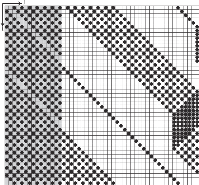
Refer to caption
Figure 9: An orbit of limit cycle class 1-2 for 111 period. The parameters are Ne=15subscript𝑁𝑒15N_{e}=15, Ni=36subscript𝑁𝑖36N_{i}=36, M=15𝑀15M=15.

III.6 Periodic orbit: class 1-γ𝛾\gamma

By generalizing the discussion in the previous section, we can show that the initial state ujt=1subscriptsuperscript𝑢𝑡𝑗1u^{t}_{j}=1 (j=3,5,,Ne,Ne+2,,2m1+Ne,2m1+2Ne+2,,2m1+2m2+2Ne,,2m1++2mγ+γNe+2,,2m1++2mγ+γNe𝑗35subscript𝑁𝑒subscript𝑁𝑒22subscript𝑚1subscript𝑁𝑒2subscript𝑚12subscript𝑁𝑒22subscript𝑚12subscript𝑚22subscript𝑁𝑒2subscript𝑚12subscript𝑚𝛾𝛾subscript𝑁𝑒22subscript𝑚12subscript𝑚𝛾𝛾subscript𝑁𝑒j=3,5,\ldots,N_{e},N_{e}+2,\ldots,2m_{1}+N_{e},2m_{1}+2N_{e}+2,\ldots,2m_{1}+2m_{2}+2N_{e},\ldots,2m_{1}+\ldots+2m_{\gamma}+\gamma N_{e}+2,\ldots,2m_{1}+\ldots+2m_{\gamma}+\gamma N_{e}) and ujt=0subscriptsuperscript𝑢𝑡𝑗0u^{t}_{j}=0 for other sites yields the periodic orbit whose properties are

T=2M+(γ1)Ne+1𝑇2𝑀𝛾1subscript𝑁𝑒1\displaystyle T=2M+(\gamma-1)N_{e}+1 (26)
Ji=2MNe+12(2M+(γ1)Ne+1)delimited-⟨⟩subscript𝐽𝑖2𝑀subscript𝑁𝑒122𝑀𝛾1subscript𝑁𝑒1\displaystyle\langle J_{i}\rangle=\frac{2M-N_{e}+1}{2(2M+(\gamma-1)N_{e}+1)} (27)
Je=2M+(γ1)(Ne1)2(2M+(γ1)Ne+1)delimited-⟨⟩subscript𝐽𝑒2𝑀𝛾1subscript𝑁𝑒122𝑀𝛾1subscript𝑁𝑒1\displaystyle\langle J_{e}\rangle=\frac{2M+(\gamma-1)(N_{e}-1)}{2(2M+(\gamma-1)N_{e}+1)} (28)

for γ>0𝛾0\gamma>0 and the necessary condition to attract this limit cycle is

Ni(γ1)Ne2M<Ni(γ2)Ne2subscript𝑁𝑖𝛾1subscript𝑁𝑒2𝑀subscript𝑁𝑖𝛾2subscript𝑁𝑒2\frac{N_{i}-(\gamma-1)N_{e}}{2}\leq M<\frac{N_{i}-(\gamma-2)N_{e}}{2} (29)

while M>Ne/2𝑀subscript𝑁𝑒2M>N_{e}/2. Here, we stress that these conditions are disjoint and cover all MN/2𝑀𝑁2M\leq N/2, i.e., this class of limit cycles is uniquely determined by the number of balls if the initial state is general.

It should be noted that these formulae of flow depend only on the number of balls and clusters and the length of the main region but not the length of the skipped region and the condition depends only on them but not the detail of each cluster.

Fig. 10 shows an example of the flow of each region versus the number of balls. We can observe that most of points are on the dashed curve which is depicted from the formula (20). This means that the orbits providing these values are general ones.

Refer to caption
Figure 10: A part of the graph of the flow in the skipped region for Nm=301subscript𝑁𝑚301N_{m}=301, Ns=700subscript𝑁𝑠700N_{s}=700. The dashed curve is depicted by the formula (20). Points are numerically calculated by definition (13).

We mention that the total number of the balls which are bumped to the skipped region in a period is Q=(2MNe+1)/2𝑄2𝑀subscript𝑁𝑒12Q=(2M-N_{e}+1)/2, which is not depend on the mode and continuous by the number of balls. The value which changes discontinuously by the number of balls is period, which is depend on the mode. This is the reason why the flow changes discontinuously.

In the last of this section, we note that by setting γ=0𝛾0\gamma=0, the flow is equal to (14). However, the period is 2MNe+12𝑀subscript𝑁𝑒12M-N_{e}+1, which is equal to twice of the number of balls in the skipped region. The real period 222 is trivially an aliquot of this system period but this is a little interesting result.

III.7 Special periodic orbits
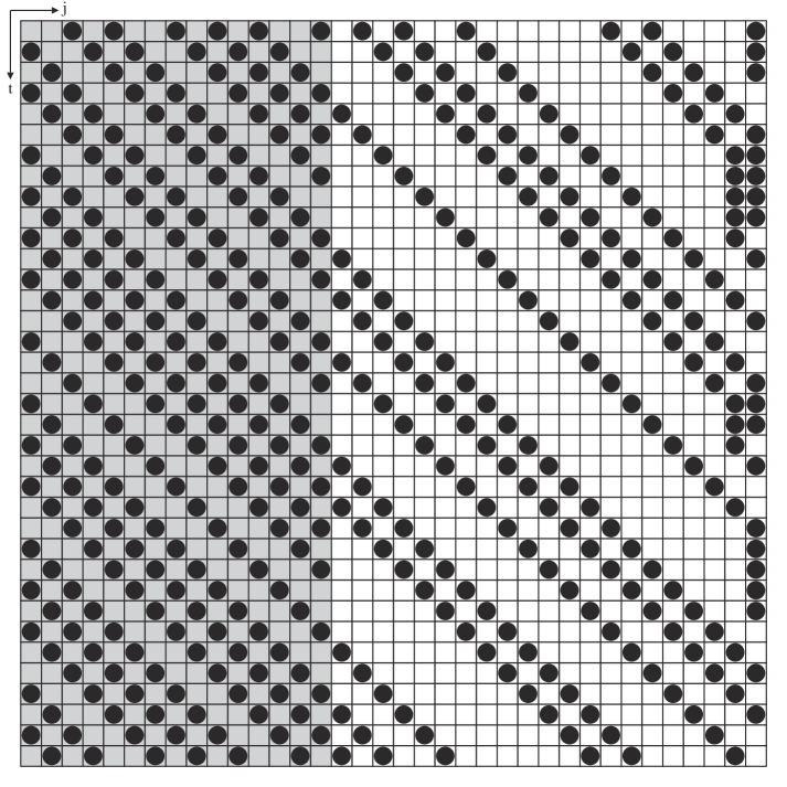
Refer to caption
Figure 11: An example of special periodic orbits. The parameters are Ne=15subscript𝑁𝑒15N_{e}=15, Ni=21subscript𝑁𝑖21N_{i}=21, M=12𝑀12M=12. The period of this limit cycle is 363636 though that of general limit cycles should be 252525. We also note that the general limit cycles also exist for this parameter.

Next we consider special periodic orbits. The observation of such orbits (See Figure 11) reveals that there are several notches in the main region, which is the major difference from the general periodic orbits. Obviously, the parity of the number of notches and Nesubscript𝑁𝑒N_{e} are the same.

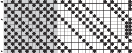
To analyze such orbits, we introduce snapshots of the orbit when a notch arrives at the top of the main region (See Fig. 12). From these snapshots, we can set α𝛼\alpha as the number of notches in the main region and γ𝛾\gamma as the number of clusters in the skipped region. We also let nisubscript𝑛𝑖n_{i} be the number of balls between i𝑖i-th and i+1𝑖1i+1-th notches for i=1,,α1𝑖1𝛼1i=1,\ldots,\alpha-1 and nαsubscript𝑛𝛼n_{\alpha} be that between α𝛼\alpha-th notch and the first interval in the skipped region, misubscript𝑚𝑖m_{i} be the number of balls of the i𝑖i-th cluster (which is the same in the last section) and lisubscript𝑙𝑖l_{i} be the length of the intervals between i𝑖i-th cluster in the skipped region and i+1𝑖1i+1-th one (See Figure 13). We note that balls in the nαsubscript𝑛𝛼n_{\alpha} and m1subscript𝑚1m_{1} are double-counted because it is convenient. After time evolutions, we can take the next snapshot and define {nj}subscriptsuperscript𝑛𝑗\{n^{\prime}_{j}\}, {mi}subscriptsuperscript𝑚𝑖\{m^{\prime}_{i}\} and {li}subscriptsuperscript𝑙𝑖\{l^{\prime}_{i}\} by the similar way.

Refer to caption
Refer to caption
Figure 12: We take snapshots for star marked states and consider the relation between snapshots.
Refer to caption
Figure 13: The definition of m𝑚m, n𝑛n. We count n𝑛n and m𝑚m for the number of balls and l𝑙l the number of empty boxes. In this case, the data are α=3𝛼3\alpha=3, γ=4𝛾4\gamma=4 and (n1,n2,n3;m1,m2,m3,m4;l1,l2,l3)=(2,3,3;2,1,2,1;2,6,4)subscript𝑛1subscript𝑛2subscript𝑛3subscript𝑚1subscript𝑚2subscript𝑚3subscript𝑚4subscript𝑙1subscript𝑙2subscript𝑙32332121264(n_{1},n_{2},n_{3};m_{1},m_{2},m_{3},m_{4};l_{1},l_{2},l_{3})=(2,3,3;2,1,2,1;2,6,4).

These variables satisfy the relation:

i=1αnim1=Neα2superscriptsubscript𝑖1𝛼subscript𝑛𝑖subscript𝑚1subscript𝑁𝑒𝛼2\displaystyle\sum_{i=1}^{\alpha}n_{i}-m_{1}=\frac{N_{e}-\alpha}{2} (30)
i=1γmi=MNeα2superscriptsubscript𝑖1𝛾subscript𝑚𝑖𝑀subscript𝑁𝑒𝛼2\displaystyle\sum_{i=1}^{\gamma}m_{i}=M-\frac{N_{e}-\alpha}{2} (31)

and the parities of α𝛼\alpha and Nesubscript𝑁𝑒N_{e} are the same.

We next consider the relationship between (n,m,l)𝑛𝑚𝑙(n,m,l) and (n,m,l)superscript𝑛superscript𝑚superscript𝑙(n^{\prime},m^{\prime},l^{\prime}). Now, we assume that the number of the notches and that of the clusters are preserved, i.e., there are no collision of clusters or no resolution of notches (we discuss the conditions later).

Since the clusters which are not last of each region are just traveling and make no collision, they just shift the order in the next snapshot. Then, we only focus on the last clusters. By the same discussion in the previous section, the last cluster in the main region separates balls staying around the main region and a new cluster in the skipped region and staying balls and the last cluster in the skipped region join together. The joining cluster of the skipped region push out the same amount of balls to the skipped region. The intervals between the currently last cluster at the skipped region and the newly generated cluster is determined by the number of going around balls of the top cluster in the main region and the next notch. Therefore, the relationship between (n,m,l)𝑛𝑚𝑙(n,m,l) and (n,m,l)superscript𝑛superscript𝑚superscript𝑙(n^{\prime},m^{\prime},l^{\prime}) expressed as:

n1=nαm1+mγsubscriptsuperscript𝑛1subscript𝑛𝛼subscript𝑚1subscript𝑚𝛾\displaystyle n^{\prime}_{1}=n_{\alpha}-m_{1}+m_{\gamma} (32)
ni=ni1subscriptsuperscript𝑛𝑖subscript𝑛𝑖1\displaystyle n^{\prime}_{i}=n_{i-1} (33)
m1=mγsubscriptsuperscript𝑚1subscript𝑚𝛾\displaystyle m^{\prime}_{1}=m_{\gamma} (34)
mi=mi1subscriptsuperscript𝑚𝑖subscript𝑚𝑖1\displaystyle m^{\prime}_{i}=m_{i-1} (35)
l1=2(nαm1)+2subscriptsuperscript𝑙12subscript𝑛𝛼subscript𝑚12\displaystyle l^{\prime}_{1}=2(n_{\alpha}-m_{1})+2 (36)
li=li1subscriptsuperscript𝑙𝑖subscript𝑙𝑖1\displaystyle l^{\prime}_{i}=l_{i-1} (37)

We define this update map from (n;m)𝑛𝑚(n;m) to (n;m)superscript𝑛superscript𝑚(n^{\prime};m^{\prime}) as F𝐹F, i.e., (n;m)=F(n;m)superscript𝑛superscript𝑚𝐹𝑛𝑚(n^{\prime};m^{\prime})=F(n;m), which is a linear one and its matrix representation is written in

(n1n2nα1nαm1m2mγ1mγ)=(1111111111)(n1n2nα1nαm1m2mγ1mγ).subscriptsuperscript𝑛1subscriptsuperscript𝑛2subscriptsuperscript𝑛𝛼1subscriptsuperscript𝑛𝛼missing-subexpressionsubscriptsuperscript𝑚1subscriptsuperscript𝑚2subscriptsuperscript𝑚𝛾1subscriptsuperscript𝑚𝛾missing-subexpressionmissing-subexpressionmissing-subexpressionmissing-subexpression11missing-subexpressionmissing-subexpressionmissing-subexpression11missing-subexpressionmissing-subexpressionmissing-subexpressionmissing-subexpressionmissing-subexpressionmissing-subexpressionmissing-subexpressionmissing-subexpressionmissing-subexpressionmissing-subexpressionmissing-subexpressionmissing-subexpressionmissing-subexpressionmissing-subexpressionmissing-subexpressionmissing-subexpressionmissing-subexpressionmissing-subexpressionmissing-subexpressionmissing-subexpression1missing-subexpressionmissing-subexpressionmissing-subexpressionmissing-subexpressionmissing-subexpressionmissing-subexpressionmissing-subexpressionmissing-subexpressionmissing-subexpressionmissing-subexpression1missing-subexpressionmissing-subexpressionmissing-subexpressionmissing-subexpressionmissing-subexpressionmissing-subexpressionmissing-subexpressionmissing-subexpressionmissing-subexpressionmissing-subexpressionmissing-subexpressionmissing-subexpressionmissing-subexpressionmissing-subexpressionmissing-subexpressionmissing-subexpressionmissing-subexpressionmissing-subexpressionmissing-subexpressionmissing-subexpressionmissing-subexpressionmissing-subexpressionmissing-subexpressionmissing-subexpressionmissing-subexpression1missing-subexpressionmissing-subexpressionmissing-subexpressionmissing-subexpressionmissing-subexpression1missing-subexpressionmissing-subexpressionmissing-subexpressionmissing-subexpressionmissing-subexpressionmissing-subexpressionmissing-subexpressionmissing-subexpressionmissing-subexpressionmissing-subexpressionmissing-subexpressionmissing-subexpressionmissing-subexpressionmissing-subexpressionmissing-subexpressionmissing-subexpressionmissing-subexpressionmissing-subexpressionmissing-subexpressionmissing-subexpression1missing-subexpressionmissing-subexpressionmissing-subexpressionmissing-subexpressionmissing-subexpressionmissing-subexpressionmissing-subexpressionmissing-subexpressionmissing-subexpressionmissing-subexpression1missing-subexpressionsubscript𝑛1subscript𝑛2subscript𝑛𝛼1subscript𝑛𝛼missing-subexpressionsubscript𝑚1subscript𝑚2subscript𝑚𝛾1subscript𝑚𝛾\left(\begin{array}[]{c}n^{\prime}_{1}\\ n^{\prime}_{2}\\ \vdots\\ n^{\prime}_{\alpha-1}\\ n^{\prime}_{\alpha}\\ \hline\cr m^{\prime}_{1}\\ m^{\prime}_{2}\\ \vdots\\ m^{\prime}_{\gamma-1}\\ m^{\prime}_{\gamma}\end{array}\right)=\left(\begin{array}[]{ccccc|ccccc}&&&&1&-1&&&&1\\ 1&&&&&&&&&\\ &\ddots&&&&&&&&\\ &&1&&&&&&&\\ &&&1&&&&&&\\ \hline\cr&&&&&&&&&1\\ &&&&&1&&&&\\ &&&&&&\ddots&&&\\ &&&&&&&1&&\\ &&&&&&&&1&\end{array}\right)\left(\begin{array}[]{c}n_{1}\\ n_{2}\\ \vdots\\ n_{\alpha-1}\\ n_{\alpha}\\ \hline\cr m_{1}\\ m_{2}\\ \vdots\\ m_{\gamma-1}\\ m_{\gamma}\end{array}\right). (38)

The eigenvalues of this matrix are e2πiμ/αsuperscript𝑒2𝜋𝑖𝜇𝛼e^{2\pi i\mu/\alpha} (μ=0,1,,α𝜇01𝛼\mu=0,1,\ldots,\alpha) and e2πiν/γsuperscript𝑒2𝜋𝑖𝜈𝛾e^{2\pi i\nu/\gamma} (ν=0,1,,γ𝜈01𝛾\nu=0,1,\ldots,\gamma).

If α𝛼\alpha and γ𝛾\gamma are co-prime, this matrix has eigenvalue 111 with algebraic multiplicity 222 but the dimension of corresponding eigenspace is also 222, that is, arbitrary initial states is decomposed by linear combination of the eigenvector. Then, by applying this map αγ𝛼𝛾\alpha\gamma times, the data finally become the same as the initial data, which is consistent with the periodicity of the system.

However, if α𝛼\alpha and γ𝛾\gamma are not co-prime, e2πiv/qsuperscript𝑒2𝜋𝑖𝑣𝑞e^{2\pi iv/q} (v=1,2,,q1𝑣12𝑞1v=1,2,\ldots,q-1) are also eigenvalues with multiplicity 222 but the dimension of the eigenspace is 1, where q=gcd(α,γ)𝑞𝛼𝛾q=\gcd(\alpha,\gamma). Then, there can be an initial state which is not expressed as a linear combination of the eigenvectors. If we take such an initial state, the system seems to behave not periodic and the data (n;m)𝑛𝑚(n;m) seem to grow as polynomial order with oscillation. However, the conditions to preserve the form of cluster break after several steps. Then, we do not consider such cases. The condition which an initial state is expressed as a linear combination of the eigenvectors is written in

m1+m1+q++m1+(d1)q=m2+m2+q++m2+(d1)q==mq+m2q++mdqsubscript𝑚1subscript𝑚1𝑞subscript𝑚1𝑑1𝑞subscript𝑚2subscript𝑚2𝑞subscript𝑚2𝑑1𝑞subscript𝑚𝑞subscript𝑚2𝑞subscript𝑚𝑑𝑞\displaystyle m_{1}+m_{1+q}+\ldots+m_{1+(d-1)q}=m_{2}+m_{2+q}+\ldots+m_{2+(d-1)q}=\ldots=m_{q}+m_{2q}+\ldots+m_{dq} (39)

where d=γ/q𝑑𝛾𝑞d=\gamma/q.


We now consider the conditions to preserve the form of clusters which is assumed in this discussion. It is required that the all clusters are in the system. Then, the one has:

1+i=1γ(2mi1)+i=1γ1liNi.1superscriptsubscript𝑖1𝛾2subscript𝑚𝑖1superscriptsubscript𝑖1𝛾1subscript𝑙𝑖subscript𝑁𝑖1+\sum_{i=1}^{\gamma}(2m_{i}-1)+\sum_{i=1}^{\gamma-1}l_{i}\leq N_{i}. (40)

Similarly to the discussion in the previous section, we next consider characteristic time which determines the behavior of the system:

  1. 1.

    The top cluster at the skipped region arrives at the last site of the skipped region:

    t0=Ns(1+i=1γ(2mi1)+i=1γ1li).subscript𝑡0subscript𝑁𝑠1superscriptsubscript𝑖1𝛾2subscript𝑚𝑖1superscriptsubscript𝑖1𝛾1subscript𝑙𝑖t_{0}=N_{s}-\left(1+\sum_{i=1}^{\gamma}(2m_{i}-1)+\sum_{i=1}^{\gamma-1}l_{i}\right). (41)
  2. 2.

    The top notch arrives at the last site of the main region:

    t1=2(nαm1)1.subscript𝑡12subscript𝑛𝛼subscript𝑚11t_{1}=2(n_{\alpha}-m_{1})-1. (42)
  3. 3.

    All the balls of the top cluster go back to the main region:

    t2=t1+2mγ1=2nα2.subscript𝑡2subscript𝑡12subscript𝑚𝛾12subscript𝑛𝛼2t_{2}=t_{1}+2m_{\gamma}-1=2n_{\alpha}-2. (43)
  4. 4.

    The second top cluster arrives at the last site of the skipped region:

    t3=Ns(1+i=1γ1(2mi1)+i=1γ2li).subscript𝑡3subscript𝑁𝑠1superscriptsubscript𝑖1𝛾12subscript𝑚𝑖1superscriptsubscript𝑖1𝛾2subscript𝑙𝑖t_{3}=N_{s}-\left(1+\sum_{i=1}^{\gamma-1}(2m_{i}-1)+\sum_{i=1}^{\gamma-2}l_{i}\right). (44)
  5. 5.

    The second notch arrives at the last of the main region:

    t4=2(nαm1+nα1).subscript𝑡42subscript𝑛𝛼subscript𝑚1subscript𝑛𝛼1t_{4}=2(n_{\alpha}-m_{1}+n_{\alpha-1}). (45)

To preserve the number of the notches and the clusters, this characteristic time must satisfy the relation (0)t0t1<t2<t3t4(0\leq)t_{0}\leq t_{1}<t_{2}<t_{3}\leq t_{4}. If not, the shape of the orbit is finally broken. For example, if t1<t0subscript𝑡1subscript𝑡0t_{1}<t_{0}, we have to add the cluster with length 0 like that in subsection E, if t4<t3subscript𝑡4subscript𝑡3t_{4}<t_{3}, notches finally resolve and if t5<t3subscript𝑡5subscript𝑡3t_{5}<t_{3}, the second top cluster catches up the top one before it goes to main region and two clusters coalesce.

However, these conditions guarantee only the existence of the next data and we need to check that the new data also satisfy those conditions again to construct periodic orbits. Repeating this procedure at most αγ𝛼𝛾\alpha\gamma times, we can check that the given initial data generate the periodic orbit.


To calculate the period and the flow, we consider the values=0αγ1n1(s)superscriptsubscript𝑠0𝛼𝛾1subscriptsuperscript𝑛𝑠1\sum_{s=0}^{\alpha\gamma-1}n^{(s)}_{1}, where (n(0);m(0))superscript𝑛0superscript𝑚0(n^{(0)};m^{(0)}) is the initial data (n;m)𝑛𝑚(n;m) and (n(s),m(s))=F(n(s1),m(s1))superscript𝑛𝑠superscript𝑚𝑠𝐹superscript𝑛𝑠1superscript𝑚𝑠1(n^{(s)},m^{(s)})=F(n^{(s-1)},m^{(s-1)}) recursively. By virtue of the rule (33) and (30):

s=0α1n1(s)mγα+2=s=0α1n1+s(α1)mγα+2=Neα2,superscriptsubscript𝑠0𝛼1subscriptsuperscript𝑛𝑠1subscript𝑚𝛾𝛼2superscriptsubscript𝑠0𝛼1subscriptsuperscript𝑛𝛼11𝑠subscript𝑚𝛾𝛼2subscript𝑁𝑒𝛼2\displaystyle\sum_{s=0}^{\alpha-1}n^{(s)}_{1}-m_{\gamma-\alpha+2}=\sum_{s=0}^{\alpha-1}n^{(\alpha-1)}_{1+s}-m_{\gamma-\alpha+2}=\frac{N_{e}-\alpha}{2}, (46)

we obtain

s=0αγ1n1(s)=r=0γ1(s=0α1n1(rα+s))=r=0γ1(s=0α1n1+s(rα))=r=0γ1(Neα2+mγrα+2),superscriptsubscript𝑠0𝛼𝛾1subscriptsuperscript𝑛𝑠1superscriptsubscript𝑟0𝛾1superscriptsubscript𝑠0𝛼1subscriptsuperscript𝑛𝑟𝛼𝑠1superscriptsubscript𝑟0𝛾1superscriptsubscript𝑠0𝛼1subscriptsuperscript𝑛𝑟𝛼1𝑠superscriptsubscript𝑟0𝛾1subscript𝑁𝑒𝛼2subscript𝑚𝛾𝑟𝛼2\displaystyle\sum_{s=0}^{\alpha\gamma-1}n^{(s)}_{1}=\sum_{r=0}^{\gamma-1}\left(\sum_{s=0}^{\alpha-1}n^{(r\alpha+s)}_{1}\right)=\sum_{r=0}^{\gamma-1}\left(\sum_{s=0}^{\alpha-1}n^{(r\alpha)}_{1+s}\right)=\sum_{r=0}^{\gamma-1}\left(\frac{N_{e}-\alpha}{2}+m_{\gamma-r\alpha+2}\right), (47)

where the index of m𝑚m takes modulo of γ𝛾\gamma. If γ𝛾\gamma and α𝛼\alpha are co-prime, γrα+2𝛾𝑟𝛼2\gamma-r\alpha+2 (r=0,1,,γ1𝑟01𝛾1r=0,1,\ldots,\gamma-1) runs on all of 1,2,,γ12𝛾1,2,\ldots,\gamma just at once. If not, γrα+2𝛾𝑟𝛼2\gamma-r\alpha+2 (r=0,1,,γ1𝑟01𝛾1r=0,1,\ldots,\gamma-1) runs on γq+2,γ2q+2,,γdq+2𝛾𝑞2𝛾2𝑞2𝛾𝑑𝑞2\gamma-q+2,\gamma-2q+2,\ldots,\gamma-dq+2 at q𝑞q times, where gcd(α,γ)=q𝛼𝛾𝑞\gcd(\alpha,\gamma)=q and d=γ/q𝑑𝛾𝑞d=\gamma/q. However, by virtue of the condition (39), finally for both cases, one has

r=0γ1mγrα+2=i=1γmi=MNeα2superscriptsubscript𝑟0𝛾1subscript𝑚𝛾𝑟𝛼2superscriptsubscript𝑖1𝛾subscript𝑚𝑖𝑀subscript𝑁𝑒𝛼2\sum_{r=0}^{\gamma-1}m_{\gamma-r\alpha+2}=\sum_{i=1}^{\gamma}m_{i}=M-\frac{N_{e}-\alpha}{2} (48)

and

s=0αγ1n1(s)=γNeα2+MNeα2=2M+(γ1)(Neα)2.superscriptsubscript𝑠0𝛼𝛾1subscriptsuperscript𝑛𝑠1𝛾subscript𝑁𝑒𝛼2𝑀subscript𝑁𝑒𝛼22𝑀𝛾1subscript𝑁𝑒𝛼2\displaystyle\sum_{s=0}^{\alpha\gamma-1}n^{(s)}_{1}=\gamma\frac{N_{e}-\alpha}{2}+M-\frac{N_{e}-\alpha}{2}=\frac{2M+(\gamma-1)(N_{e}-\alpha)}{2}. (49)

The period of the oribit is calculated by summing the time to transit each snapshot. By virtue of the similar discussion in the section C, the time to transit from the initial state to the next state satisfying u0t=u1t=0subscriptsuperscript𝑢𝑡0subscriptsuperscript𝑢𝑡10u^{t}_{0}=u^{t}_{1}=0 is 2n1+12subscript𝑛112n_{1}+1. Then, if gcd(α,γ)=1𝛼𝛾1\gcd(\alpha,\gamma)=1, the period is

T=s=0αγ1(2n1(s)+1).𝑇superscriptsubscript𝑠0𝛼𝛾12subscriptsuperscript𝑛𝑠11T=\sum_{s=0}^{\alpha\gamma-1}(2n^{(s)}_{1}+1). (50)

and due to (49), the period of this orbit is expressed as

T=2M+(γ1)Ne+α𝑇2𝑀𝛾1subscript𝑁𝑒𝛼T=2M+(\gamma-1)N_{e}+\alpha (51)

In the case of gcd(α,γ)=q>1𝛼𝛾𝑞1\gcd(\alpha,\gamma)=q>1, the real period of this system obtained by T/q𝑇𝑞T/q because the same snapshot update repeats just q𝑞q times.

The flow is also calculated by summing the number of emitted balls from the main region to the skipped region for transitioning each snapshot and dividing this sum by the period and finally written in

Js=s=0αγ1m1(s)T=α(2MNe+α)2(2M+(γ1)Ne+α)delimited-⟨⟩subscript𝐽𝑠superscriptsubscript𝑠0𝛼𝛾1subscriptsuperscript𝑚𝑠1𝑇𝛼2𝑀subscript𝑁𝑒𝛼22𝑀𝛾1subscript𝑁𝑒𝛼\displaystyle\langle J_{s}\rangle=\frac{\sum_{s=0}^{\alpha\gamma-1}m^{(s)}_{1}}{T}=\frac{\alpha(2M-N_{e}+\alpha)}{2(2M+(\gamma-1)N_{e}+\alpha)} (52)
Jm=s=0αγ1n1(s)T=2M+(γ1)(Neα)2(2M+(γ1)Ne+α),delimited-⟨⟩subscript𝐽𝑚superscriptsubscript𝑠0𝛼𝛾1subscriptsuperscript𝑛𝑠1𝑇2𝑀𝛾1subscript𝑁𝑒𝛼22𝑀𝛾1subscript𝑁𝑒𝛼\displaystyle\langle J_{m}\rangle=\frac{\sum_{s=0}^{\alpha\gamma-1}n^{(s)}_{1}}{T}=\frac{2M+(\gamma-1)(N_{e}-\alpha)}{2(2M+(\gamma-1)N_{e}+\alpha)}, (53)

which agrees the result of the numerical simulation. These formulae of the flow preserves even if the real period is shorter.

The formulae of the flow depends only on the number of balls, clusters and notches and the length of the main region, similarly to those in the last section. However, the condition depends on the detail of the data.

FIG 14 is partially magnified of FIG 7. The dashed line is the theoretical value of the flow of general periodic orbits and several points are out of this curve, which corresponds the special periodic orbits. The dotted line is that of the special periodic orbits for α=3𝛼3\alpha=3 and γ=7𝛾7\gamma=7. Therefore, we can confirm that those exceptional data correspond the special periodic orbits with 3 notches and 7 clusters.

Refer to caption
Figure 14: A part of the graph of the flow in the skipped region for Nm=301subscript𝑁𝑚301N_{m}=301, Ns=700subscript𝑁𝑠700N_{s}=700. The dashed curve are by (52) for α=3𝛼3\alpha=3, γ=7𝛾7\gamma=7.

The result in this section are finally reduced to that in the previous section when setting α=1𝛼1\alpha=1.

We can also apply this approach when Nmsubscript𝑁𝑚N_{m} is even. In this case, the balls in the skipped region can go back to the main region differently from the general orbit (See Fig. 15). The limit cycle where the balls at the skipped region creates jams and never go back to main region is considered as that in the case α=0𝛼0\alpha=0.

Refer to caption
Figure 15: An example of special limit cycles for the even length main region. The system parameters are Ne=14subscript𝑁𝑒14N_{e}=14, Ni=21subscript𝑁𝑖21N_{i}=21, M=10𝑀10M=10.

The evolution rule of data n𝑛n and m𝑚m also holds even if some of n𝑛n and m𝑚m take 00. However, the correspondence between the state ujtsubscriptsuperscript𝑢𝑡𝑗u^{t}_{j} and the data becomes more complicated for such cases. For example, the initial state in the Figure 4 seems to have 2 notches and 1 cluster but α=3𝛼3\alpha=3 and γ=5𝛾5\gamma=5 (under this settings, the evolution of the system is well explained). The relation (36) helps to obtain the real number of the notches and clusters. If the real length of interval between two clusters is different from the length obtained from (36), there is the position where null clusters should be inserted.

IV Dynamics with several skipped regions

Our approach in the previous section is also applicable to analyze periodic orbits for the system for K2𝐾2K\geq 2 (i.e. with several jumping sites). Observing the dynamics of orbits shows that we set the sites from ιk1subscript𝜄𝑘1\iota_{k-1}-th to ϵksubscriptitalic-ϵ𝑘\epsilon_{k}-th one as k𝑘k-th main region and from (ϵk+1)subscriptitalic-ϵ𝑘1(\epsilon_{k}+1)-th to (ιk1)subscript𝜄𝑘1(\iota_{k}-1)-th as k𝑘k-th skipped region for 1kK1𝑘𝐾1\leq k\leq K which is similar to the case of K=1𝐾1K=1. This means that there are several main and skipped regions. We note that the number of main regions and skipped regions are trivially the same. In fact, the topology of the path for this system is depicted in FIG. 16 and the system consists on one main region and two detours in mid-course of the main region.

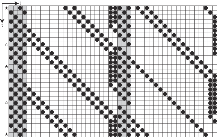
Refer to caption
Figure 16: A topological representation of two main and skipped region system.
Refer to caption
Figure 17: An example of periodic orbits for two main and skipped regions. The time when the notch arrived at the top of the first main region is filled-star marked and that when the notch arrived at the top of the second is outline-star marked.

Let us construct the general periodic orbits. Similarly to the discussion in the last section, we focus on the behavior of the notch and take snapshots of orbits when it arrives at the top of each main region and we consider the mappings for transition between these snapshots. For example, in the case of K=2𝐾2K=2, we take two types of snapshots of an orbit (See figure 17). We define n𝑛n as the number of balls forming the cluster in the main region and misubscript𝑚𝑖m_{i} as that forming i𝑖i-th cluster in the first skipped region and μisubscript𝜇𝑖\mu_{i} as that forming i𝑖i-th cluster in the second skipped region. (See Figures 18 and 19)

Refer to caption
Figure 18: Definition of the data for the filled-star marked states. In this example, the data is (n;m1,m2;μ1,μ2)=(4;1,2;1,3)𝑛subscript𝑚1subscript𝑚2subscript𝜇1subscript𝜇241213(n;m_{1},m_{2};\mu_{1},\mu_{2})=(4;1,2;1,3).
Refer to caption
Figure 19: Definition of the data for the outline-star marked states. In this example, the data is (n;m1,m2;μ1,μ2)=(5;2,1;1,3)superscript𝑛subscriptsuperscript𝑚1subscriptsuperscript𝑚2subscriptsuperscript𝜇1subscriptsuperscript𝜇252113(n^{\prime};m^{\prime}_{1},m^{\prime}_{2};\mu^{\prime}_{1},\mu^{\prime}_{2})=(5;2,1;1,3).

If the initial data (n;m1,,mγ;μ1,,μγ)𝑛subscript𝑚1subscript𝑚𝛾subscript𝜇1subscript𝜇superscript𝛾(n;m_{1},\ldots,m_{\gamma};\mu_{1},\ldots,\mu_{\gamma^{\prime}}) is given, the data (n;m1,,mγ;μ1,,μγ)superscript𝑛subscriptsuperscript𝑚1subscriptsuperscript𝑚𝛾subscriptsuperscript𝜇1subscriptsuperscript𝜇superscript𝛾(n^{\prime};m^{\prime}_{1},\ldots,m^{\prime}_{\gamma};\mu^{\prime}_{1},\ldots,\mu^{\prime}_{\gamma^{\prime}}) is expressed as

(nm1m2mγ1mγμ1μ2μγ1μγ)=(11111111111)(nm1m2mγ1mγμ1μ2μγ1μγ).superscript𝑛missing-subexpressionsubscriptsuperscript𝑚1subscriptsuperscript𝑚2subscriptsuperscript𝑚𝛾1subscriptsuperscript𝑚𝛾missing-subexpressionsubscriptsuperscript𝜇1subscriptsuperscript𝜇2subscriptsuperscript𝜇superscript𝛾1subscriptsuperscript𝜇superscript𝛾1missing-subexpressionmissing-subexpressionmissing-subexpressionmissing-subexpression11missing-subexpressionmissing-subexpressionmissing-subexpressionmissing-subexpressionmissing-subexpressionmissing-subexpressionmissing-subexpressionmissing-subexpressionmissing-subexpressionmissing-subexpressionmissing-subexpressionmissing-subexpressionmissing-subexpressionmissing-subexpressionmissing-subexpressionmissing-subexpression1missing-subexpressionmissing-subexpressionmissing-subexpressionmissing-subexpressionmissing-subexpressionmissing-subexpressionmissing-subexpressionmissing-subexpressionmissing-subexpressionmissing-subexpressionmissing-subexpression1missing-subexpressionmissing-subexpressionmissing-subexpressionmissing-subexpressionmissing-subexpressionmissing-subexpressionmissing-subexpressionmissing-subexpressionmissing-subexpressionmissing-subexpressionmissing-subexpressionmissing-subexpressionmissing-subexpressionmissing-subexpressionmissing-subexpressionmissing-subexpressionmissing-subexpressionmissing-subexpressionmissing-subexpressionmissing-subexpressionmissing-subexpressionmissing-subexpression1missing-subexpressionmissing-subexpressionmissing-subexpressionmissing-subexpressionmissing-subexpressionmissing-subexpressionmissing-subexpressionmissing-subexpressionmissing-subexpressionmissing-subexpressionmissing-subexpression1missing-subexpressionmissing-subexpressionmissing-subexpressionmissing-subexpressionmissing-subexpressionmissing-subexpressionmissing-subexpressionmissing-subexpressionmissing-subexpressionmissing-subexpressionmissing-subexpressionmissing-subexpressionmissing-subexpressionmissing-subexpressionmissing-subexpressionmissing-subexpressionmissing-subexpressionmissing-subexpressionmissing-subexpressionmissing-subexpressionmissing-subexpressionmissing-subexpressionmissing-subexpressionmissing-subexpressionmissing-subexpressionmissing-subexpression1missing-subexpressionmissing-subexpressionmissing-subexpressionmissing-subexpressionmissing-subexpressionmissing-subexpression1missing-subexpressionmissing-subexpressionmissing-subexpressionmissing-subexpressionmissing-subexpressionmissing-subexpressionmissing-subexpressionmissing-subexpressionmissing-subexpressionmissing-subexpressionmissing-subexpressionmissing-subexpressionmissing-subexpressionmissing-subexpressionmissing-subexpressionmissing-subexpressionmissing-subexpressionmissing-subexpressionmissing-subexpressionmissing-subexpressionmissing-subexpressionmissing-subexpression1missing-subexpressionmissing-subexpressionmissing-subexpressionmissing-subexpressionmissing-subexpressionmissing-subexpressionmissing-subexpressionmissing-subexpressionmissing-subexpressionmissing-subexpressionmissing-subexpression1missing-subexpression𝑛missing-subexpressionsubscript𝑚1subscript𝑚2subscript𝑚𝛾1subscript𝑚𝛾missing-subexpressionsubscript𝜇1subscript𝜇2subscript𝜇superscript𝛾1subscript𝜇superscript𝛾\left(\begin{array}[]{c}n^{\prime}\\ \hline\cr m^{\prime}_{1}\\ m^{\prime}_{2}\\ \vdots\\ m^{\prime}_{\gamma-1}\\ m^{\prime}_{\gamma}\\ \hline\cr\mu^{\prime}_{1}\\ \mu^{\prime}_{2}\\ \vdots\\ \mu^{\prime}_{\gamma^{\prime}-1}\\ \mu^{\prime}_{\gamma^{\prime}}\end{array}\right)=\left(\begin{array}[]{c|ccccc|ccccc}1&&&&&1&-1&&&&\\ \hline\cr&1&&&&&&&&&\\ &&1&&&&&&&&\\ &&&\ddots&&&&&&&\\ &&&&1&&&&&&\\ &&&&&1&&&&&\\ \hline\cr&&&&&&&&&&1\\ &&&&&&1&&&&\\ &&&&&&&\ddots&&&\\ &&&&&&&&1&&\\ &&&&&&&&&1&\end{array}\right)\left(\begin{array}[]{c}n\\ \hline\cr m_{1}\\ m_{2}\\ \vdots\\ m_{\gamma-1}\\ m_{\gamma}\\ \hline\cr\mu_{1}\\ \mu_{2}\\ \vdots\\ \mu_{\gamma^{\prime}-1}\\ \mu_{\gamma^{\prime}}\end{array}\right). (54)

Let the data when the notch which departed from the second main region arrives at the first main region be (n~;m~1,,m~γ;μ~1,,μ~γ)~𝑛subscript~𝑚1subscript~𝑚𝛾subscript~𝜇1subscript~𝜇superscript𝛾(\tilde{n};\tilde{m}_{1},\ldots,\tilde{m}_{\gamma};\tilde{\mu}_{1},\ldots,\tilde{\mu}_{\gamma^{\prime}}) and the relation between these data and (n;m1,,mγ;μ1,,μγ)superscript𝑛subscriptsuperscript𝑚1subscriptsuperscript𝑚𝛾subscriptsuperscript𝜇1subscriptsuperscript𝜇superscript𝛾(n^{\prime};m^{\prime}_{1},\ldots,m^{\prime}_{\gamma};\mu^{\prime}_{1},\ldots,\mu^{\prime}_{\gamma^{\prime}}) is written in

(n~m~1m~2m~γ1m~γμ~1μ~2μ~γ1μ~γ)=(11111111111)(nm1m2mγ1mγμ1μ2μγ1μγ).~𝑛missing-subexpressionsubscript~𝑚1subscript~𝑚2subscript~𝑚𝛾1subscript~𝑚𝛾missing-subexpressionsubscript~𝜇1subscript~𝜇2subscript~𝜇superscript𝛾1subscript~𝜇superscript𝛾11missing-subexpressionmissing-subexpressionmissing-subexpressionmissing-subexpressionmissing-subexpressionmissing-subexpressionmissing-subexpressionmissing-subexpression1missing-subexpressionmissing-subexpressionmissing-subexpressionmissing-subexpressionmissing-subexpressionmissing-subexpressionmissing-subexpressionmissing-subexpressionmissing-subexpressionmissing-subexpressionmissing-subexpressionmissing-subexpressionmissing-subexpressionmissing-subexpressionmissing-subexpressionmissing-subexpression1missing-subexpressionmissing-subexpressionmissing-subexpressionmissing-subexpressionmissing-subexpressionmissing-subexpression1missing-subexpressionmissing-subexpressionmissing-subexpressionmissing-subexpressionmissing-subexpressionmissing-subexpressionmissing-subexpressionmissing-subexpressionmissing-subexpressionmissing-subexpressionmissing-subexpressionmissing-subexpressionmissing-subexpressionmissing-subexpressionmissing-subexpressionmissing-subexpressionmissing-subexpressionmissing-subexpressionmissing-subexpressionmissing-subexpressionmissing-subexpressionmissing-subexpression1missing-subexpressionmissing-subexpressionmissing-subexpressionmissing-subexpressionmissing-subexpressionmissing-subexpressionmissing-subexpressionmissing-subexpressionmissing-subexpressionmissing-subexpressionmissing-subexpression1missing-subexpressionmissing-subexpressionmissing-subexpressionmissing-subexpressionmissing-subexpressionmissing-subexpressionmissing-subexpressionmissing-subexpressionmissing-subexpressionmissing-subexpressionmissing-subexpressionmissing-subexpressionmissing-subexpressionmissing-subexpressionmissing-subexpressionmissing-subexpressionmissing-subexpressionmissing-subexpressionmissing-subexpressionmissing-subexpressionmissing-subexpressionmissing-subexpressionmissing-subexpression1missing-subexpressionmissing-subexpressionmissing-subexpressionmissing-subexpressionmissing-subexpressionmissing-subexpressionmissing-subexpressionmissing-subexpressionmissing-subexpressionmissing-subexpressionmissing-subexpression1missing-subexpressionmissing-subexpressionmissing-subexpressionmissing-subexpressionmissing-subexpressionmissing-subexpressionmissing-subexpressionmissing-subexpressionmissing-subexpressionmissing-subexpressionmissing-subexpressionmissing-subexpressionmissing-subexpressionmissing-subexpressionmissing-subexpressionmissing-subexpressionmissing-subexpressionmissing-subexpressionmissing-subexpressionmissing-subexpressionmissing-subexpressionmissing-subexpression1missing-subexpressionmissing-subexpressionmissing-subexpressionmissing-subexpressionmissing-subexpressionmissing-subexpressionmissing-subexpressionmissing-subexpressionmissing-subexpressionmissing-subexpressionmissing-subexpression1superscript𝑛missing-subexpressionsubscriptsuperscript𝑚1subscriptsuperscript𝑚2subscriptsuperscript𝑚𝛾1subscriptsuperscript𝑚𝛾missing-subexpressionsubscriptsuperscript𝜇1subscriptsuperscript𝜇2subscriptsuperscript𝜇superscript𝛾1subscriptsuperscript𝜇superscript𝛾\left(\begin{array}[]{c}\tilde{n}\\ \hline\cr\tilde{m}_{1}\\ \tilde{m}_{2}\\ \vdots\\ \tilde{m}_{\gamma-1}\\ \tilde{m}_{\gamma}\\ \hline\cr\tilde{\mu}_{1}\\ \tilde{\mu}_{2}\\ \vdots\\ \tilde{\mu}_{\gamma^{\prime}-1}\\ \tilde{\mu}_{\gamma^{\prime}}\end{array}\right)=\left(\begin{array}[]{c|ccccc|ccccc}1&-1&&&&&&&&&1\\ \hline\cr&&&&&1&&&&&\\ &1&&&&&&&&&\\ &&\ddots&&&&&&&&\\ &&&1&&&&&&&\\ &&&&1&&&&&&\\ \hline\cr&&&&&&1&&&&\\ &&&&&&&1&&&\\ &&&&&&&&\ddots&&\\ &&&&&&&&&1&\\ &&&&&&&&&&1\end{array}\right)\left(\begin{array}[]{c}n^{\prime}\\ \hline\cr m^{\prime}_{1}\\ m^{\prime}_{2}\\ \vdots\\ m^{\prime}_{\gamma-1}\\ m^{\prime}_{\gamma}\\ \hline\cr\mu^{\prime}_{1}\\ \mu^{\prime}_{2}\\ \vdots\\ \mu^{\prime}_{\gamma^{\prime}-1}\\ \mu^{\prime}_{\gamma^{\prime}}\end{array}\right). (55)

Then, when the notch comes back to the top of the first main region again, the matrix representation of the update of m𝑚m and n𝑛n is written in the product of two matrices representations expressed as

(n~m~1m~2m~γ1m~γμ~1μ~2μ~γ1μ~γ)=(11111111111)(nm1m2mγ1mγμ1μ2μγ1μγ)~𝑛missing-subexpressionsubscript~𝑚1subscript~𝑚2subscript~𝑚𝛾1subscript~𝑚𝛾missing-subexpressionsubscript~𝜇1subscript~𝜇2subscript~𝜇superscript𝛾1subscript~𝜇superscript𝛾11missing-subexpressionmissing-subexpressionmissing-subexpression1missing-subexpressionmissing-subexpressionmissing-subexpressionmissing-subexpressionmissing-subexpressionmissing-subexpressionmissing-subexpressionmissing-subexpressionmissing-subexpressionmissing-subexpressionmissing-subexpressionmissing-subexpressionmissing-subexpressionmissing-subexpressionmissing-subexpressionmissing-subexpressionmissing-subexpressionmissing-subexpressionmissing-subexpressionmissing-subexpressionmissing-subexpression1missing-subexpressionmissing-subexpressionmissing-subexpressionmissing-subexpressionmissing-subexpressionmissing-subexpression1missing-subexpressionmissing-subexpressionmissing-subexpressionmissing-subexpressionmissing-subexpressionmissing-subexpressionmissing-subexpressionmissing-subexpressionmissing-subexpressionmissing-subexpressionmissing-subexpressionmissing-subexpressionmissing-subexpressionmissing-subexpressionmissing-subexpressionmissing-subexpressionmissing-subexpressionmissing-subexpressionmissing-subexpressionmissing-subexpressionmissing-subexpressionmissing-subexpression1missing-subexpressionmissing-subexpressionmissing-subexpressionmissing-subexpressionmissing-subexpressionmissing-subexpressionmissing-subexpressionmissing-subexpressionmissing-subexpressionmissing-subexpressionmissing-subexpression1missing-subexpressionmissing-subexpressionmissing-subexpressionmissing-subexpressionmissing-subexpressionmissing-subexpressionmissing-subexpressionmissing-subexpressionmissing-subexpressionmissing-subexpressionmissing-subexpressionmissing-subexpressionmissing-subexpressionmissing-subexpressionmissing-subexpressionmissing-subexpressionmissing-subexpressionmissing-subexpressionmissing-subexpressionmissing-subexpressionmissing-subexpressionmissing-subexpressionmissing-subexpressionmissing-subexpressionmissing-subexpressionmissing-subexpressionmissing-subexpression1missing-subexpressionmissing-subexpressionmissing-subexpressionmissing-subexpressionmissing-subexpressionmissing-subexpression1missing-subexpressionmissing-subexpressionmissing-subexpressionmissing-subexpressionmissing-subexpressionmissing-subexpressionmissing-subexpressionmissing-subexpressionmissing-subexpressionmissing-subexpressionmissing-subexpressionmissing-subexpressionmissing-subexpressionmissing-subexpressionmissing-subexpressionmissing-subexpressionmissing-subexpressionmissing-subexpressionmissing-subexpressionmissing-subexpressionmissing-subexpressionmissing-subexpression1missing-subexpressionmissing-subexpressionmissing-subexpressionmissing-subexpressionmissing-subexpressionmissing-subexpressionmissing-subexpressionmissing-subexpressionmissing-subexpressionmissing-subexpressionmissing-subexpression1missing-subexpression𝑛missing-subexpressionsubscript𝑚1subscript𝑚2subscript𝑚𝛾1subscript𝑚𝛾missing-subexpressionsubscript𝜇1subscript𝜇2subscript𝜇superscript𝛾1subscript𝜇superscript𝛾\left(\begin{array}[]{c}\tilde{n}\\ \hline\cr\tilde{m}_{1}\\ \tilde{m}_{2}\\ \vdots\\ \tilde{m}_{\gamma-1}\\ \tilde{m}_{\gamma}\\ \hline\cr\tilde{\mu}_{1}\\ \tilde{\mu}_{2}\\ \vdots\\ \tilde{\mu}_{\gamma^{\prime}-1}\\ \tilde{\mu}_{\gamma^{\prime}}\end{array}\right)=\left(\begin{array}[]{c|ccccc|ccccc}1&-1&&&&1&&&&&\\ \hline\cr&&&&&1&&&&&\\ &1&&&&&&&&&\\ &&\ddots&&&&&&&&\\ &&&1&&&&&&&\\ &&&&1&&&&&&\\ \hline\cr&&&&&&&&&&1\\ &&&&&&1&&&&\\ &&&&&&&\ddots&&&\\ &&&&&&&&1&&\\ &&&&&&&&&1&\end{array}\right)\left(\begin{array}[]{c}n\\ \hline\cr m_{1}\\ m_{2}\\ \vdots\\ m_{\gamma-1}\\ m_{\gamma}\\ \hline\cr\mu_{1}\\ \mu_{2}\\ \vdots\\ \mu_{\gamma^{\prime}-1}\\ \mu_{\gamma^{\prime}}\end{array}\right) (56)

The eigenvalues of this matrix are all roots of unity and the dimension of each eigenspace is equal to its algebraic multiplicity.

By virtue of the similar approach in the previous sections, we can also obtain the flow and period of these periodic orbits and the condition that orbits hold. However, differently from the case K=1𝐾1K=1, the flow depends on the length of the skipped regions and the detail of the data. Furthermore, we observed that there is a possibility that two general periodic orbits co-exists (See Fig. 20).
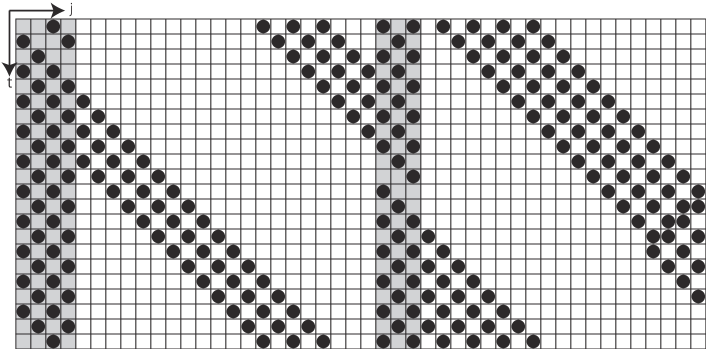
Refer to caption
Figure 20: Another example of periodic orbits for two main and skipped regions. The system parameters and the number of balls are the same as those of Fig. 17 and only one notch appears in the main region. However, the number of clusters are different.

This approach is difficult to be applied for special periodic orbits for which there appear several clusters in the main region because the notch affecting the dynamics depends on the initial state and it is difficult to determine such a notch. We believe that this difficulty is the equivalent as to analyze the orbit directly.

V Concluding Remarks

In this paper, we considered the dynamics for the simplified version of the path-preference model. We discuss the property for a class of limit cycles, which are raised by general initial states, for example, the conditions of system parameters where the orbit is attracted by one of them and the exact value of the flow in each part which depend only on the length of each part and the number of balls.

We pay attention the state where the notch in the main region is at the top. That is, we focus on the subset of states S0={u{0,1}Nu0=u1=0}subscript𝑆0conditional-set𝑢superscript01𝑁subscript𝑢0subscript𝑢10S_{0}=\{u\in\{0,1\}^{N}\mid u_{0}=u_{1}=0\} and express the change of the state between two states which an orbit started from the intersection with S0subscript𝑆0S_{0} and the next intersection after this orbit departed from S0subscript𝑆0S_{0} to understand the behavior of the orbit. This is nothing but the cellular automaton analogue of the idea of Poincaré section and Poincaré map in the continuous time dynamical systems.

Generally, it is difficult to apply the concept of Poincaré section to discrete dynamical systems naively because the orbit is discrete. However, in cellular automata, dependent variables are also discrete. Therefore, the analogue of the section can be defined naturally because there is a case where a discrete analogue of continuity of orbits can be defined naturally.

We set the time evolution rule of the system deterministic and containing a symmetry. Due to such settings, we have to mention that the behavior of orbits becomes different by the parity for the length of the main region. Therefore, it is hard to say that our analysis result can apply directly to that of the real dynamics for living systems. However, by customizing the settings of this system, we can consider other cellular automaton models as the variations to weaken such a parity and it is expected that the dynamics of these models can apply to analysis for real dynamics.

For example, let us introduce the move prior rule which is described in Section 2. The flow does not seem to change discontinuously by the number of balls in the numerical simulation. However, the dynamics is more complex than that of the jump prior rule. There is a limit cycle with ten billion order period for Nm=30subscript𝑁𝑚30N_{m}=30 and Ns=71subscript𝑁𝑠71N_{s}=71. To take such a long period, the dynamics contains some complicated structures.

Refer to caption
Figure 21: The graph of the flow in the skipped region Jsdelimited-⟨⟩subscript𝐽𝑠\langle J_{s}\rangle for the move prior rule path-preference cellular automaton where Nm=301subscript𝑁𝑚301N_{m}=301 and Ns=700subscript𝑁𝑠700N_{s}=700.

We can also introduce some stochastic factors for this model. The most famous one is in the moving process to the next site. However, we consider the case where the ball at the end of the main region jumps to the top of it or moves to the top of the skipped region stochastically. In this case, the flow loses discontinuousness for the number of balls. If jump probablity p=0𝑝0p=0, the dynamics is nothing but that of the TASEP and if 0<p<10𝑝10<p<1, the dynamics behaves intermediate one between the TASEP (p=0𝑝0p=0) and that described mainly in this paper (p=1𝑝1p=1). However, the analysis for this model is further difficult problem because we cannot introduce the mean field approximation method like that of the ASEP and Statistical dynamics methods require sufficient length of the system to ignore the effect of special sites, for example, bifurcating or confluence ones.

Acknowledgements

We would like to thank Professor Tetsuji Tokihiro and Professor Youichiro Wada for helpful comments. This research is supported by Platform for Dynamic Approaches to Living System (the Platform Project for Supporting in Drug Discovery and Life Science Research) from the Ministry of Education, Culture, Sports, Science (MEXT) and Technology, Japan, and Japan Agency for Medical Research and Development (AMED). This work is also partially supported by the JPSJ KAKENHI Grant Number 17K14199.

References

  • [1] S. Wolfram, A New Kind of Science (Wolfram Media, Champaign, IL, 2002).
  • [2] V. Belitsky and P. A. Ferrari, P. A. J Stat Phys 80, 517 (1995).
  • [3] C. Macdonald, J. Gibbs and A. Pipkin, Biopolymers 6, 1 (1968).
  • [4] B. Derrida, Phys. Rep. 301, 65 (1998).
  • [5] T. Tokihiro, D. Takahashi, J. Matsukidaira, and J. Satsuma, Phys. Rev. Lett., 76:3247–3250, 1996.
  • [6] A. Schadschneider and M. Schreckenberg, J. Phys. A: Math Gen., 26, L679 (1993).
  • [7] Y. Ohta, A. Nishiyama, et al., Phys. Rev. E, 86, 021918 (2012).
  • [8] P. R. Cook, Principles of Nuclear Structure and Function (Wiley-Liss, New York, 2001).
  • [9] A. Papantonis, J. D. Larkin, Y. Wada, Y. Ohta, S. Ihara, T. Kodama and P. R. Cook, PLoS Biol., 8, e1000419 (2010).
  • [10] P. Fraser and W. Bickmore, Nature (London) 447, 413 (2007).
  • [11] Y. Ohta, T. Kodama and S. Ihara, Phys. Rev. E 84, 041922 (2011).
  • [12] T. Tripathi and D. Chowdhury, Phys. Rev. E 77, 011921 (2008).
  • [13] T. Tripathi, G. M. Schüz and D. Chowdhury, J. Stat. Mech: Theo. Exper. (2009) P08018.
  • [14] J. G. Brankov, N. C. Pesheva and N. Zh. Bunzarova, arXiv:0803.2625
  • [15] H. Negami, private communication.
  • [16] T. Tannai and K. Nishinari J. Cell. Autom. 11, 363–375 (2016).