Conjugacies provided by fractal transformations I : Conjugate measures, Hilbert spaces, orthogonal expansions, and flows, on self-referential spaces.

Abstract.

Theorems and explicit examples are used to show how transformations between self-similar sets (general sense) may be continuous almost everywhere with respect to stationary measures on the sets and may be used to carry well known flows and spectral analysis over from familiar settings to new ones. The focus of this work is on a number of surprising applications including (i) what we call fractal Fourier analysis, in which the graphs of the basis functions are Cantor sets, being discontinuous at a countable dense set of points, yet have very good approximation properties; (ii) Lebesgue measure-preserving flows, on polygonal laminas, whose wave-fronts are fractals. The key idea is to exploit fractal transformations to provide unitary transformations between Hilbert spaces defined on attractors of iterated function systems. Some of the examples relate to work of Oxtoby and Ulam concerning ergodic flows on regions bounded by polygons.

1. Introduction

In this paper we provide results and explicit examples to show how transformations between some fractals, and other self-referential sets, may both be continuous almost everywhere and map well-known flows and spectral analysis from familiar settings to new ones. Our focus is on a number of surprising applications including: (i) what we call ”fractal Fourier analysis”, in which the basis functions are discontinuous at a countable dense set of points of a real interval, yet have good approximation properties; (ii) Lebesgue measure-preserving flows on tori whose wave-fronts are fractal curves.

The key idea is to exploit fractal transformations to provide unitary transformations between Hilbert spaces defined on attractors of iterated function systems. Some of our examples relate to the work of Oxtoby and Ulam [22], concerning ergodic flows on real geometrical domains.

Let $A_{F}$ and $A_{G}$ be non-overlapping attractors of two contractive iterated function systems (IFSs), $F$ and $G$ respectively. We give conditions under which the fractal transformation $T_{FG}:A_{F}\rightarrow A_{G}$ (defined in Section 2) is measureable and continuous almost everywhere with respect to any stationary measure $\mu_{F}$ (defined in Section 2). We show that $T_{FG}$ yields an isometry $U_{FG}:\mathcal{L}^{2}(A_{F},\mu_{F})\rightarrow\mathcal{L}^{2}(A_{G},\mu_{G}))$, where $\mu_{F}$ and $\mu_{G}$ are a corresponding pair of stationary measures. If $L_{F}:D_{F}\subset\mathcal{L}^{2}(A_{F},\mu_{F})\rightarrow\mathcal{L}^{2}(A_{F},\mu_{F})$ is a linear operator with dense domain $D_{F},$ then

$$L_{G}:=U_{FG}L_{F}U_{GF}$$

is a linear operator on $\mathcal{L}^{2}(A_{G},\mu_{G})$ with dense domain $T_{FG}(D_{F})$. If $L_{F}$ is self-adjoint, then so is $L_{G}$. In some cases $\mu_{F}$ is Lebesgue measure on a subset of $\mathbb{R}^{n}$ such as line segment, a filled triangle, or a cube; and in other cases it a uniform measure on a fractal such as a Sierpinski triangle. In these cases, familiar differential and integral equations, including those associated with Laplacians on post critically finite (p.c.f.) fractals [19, 28], can be transformed to yield interesting counterparts on other (not necessarily p.c.f.) fractals.

By way of examples (i) we introduce what we call ”fractal Fourier analysis”, in which the basis functions are discontinuous at a countable dense set of points, yet have good approximation properties including overcoming the edge-effect problem that besets standard Fourier approximation; and (ii) we introduce and exemplify certain flows on self-similar sets, we provide rough versions of flows on tori, and we exhibit the solution of a heat equation on a rough filled triangle, with Dirichlet boundary conditions.

2. Fractal transformations and invariant measures

This section introduces some essential concepts that run throughout the paper, including the invariant measure of an IFS with probabilities, called a $p$-measure, and fractal transformations from the attractor of one IFS to the attractor of another. The main result of this section are Theorem 2.1 which states that if an attractor is not equal to its dynamical boundary, then all $p$-measures of the critical set, the dynamical boundary, and the forward orbit of overlap set under the IFS (which we call the inner boundary), are zero; and Theorem 2.3 which states that a fractal transformation between non-overlapping attractors is measurable and continuous almost everywhere with respect to every $p$-measure, and that a such a fractal transformation is $p$-measure preserving.

2.1. Non-Overlapping Attractors and Fractal Transformations

The purpose of this subsection is to define the central notions of non-overlapping attractor and fractal transformation from one attractor to another.

Let $\mathbb{N=\{}1,2,3,...\}$ and $\mathbb{N}_{0}=\{0,1,2,...\}$. Throughout this paper we restrict attention to iterated function systems (IFSs) of the form

$$F=\{X;f_{1},f_{2},...,f_{N}\}$$

where $N\in\mathbb{N}$ is fixed, $X$ is a complete metric space, and $f_{i}:X\rightarrow X$ is a contraction for all $i\in I:=\{1,2,...,N\}$. By contraction we mean there is $\lambda\in[0,1)$, such that $d_{\mathbb{X}}(f_{i}(x),f_{i}(y))\leq\lambda d_{\mathbb{X}}(x,y)$ for all $x,y\in X$, for all $i\in I$.

Define $F^{-1}:2^{A}\rightarrow 2^{A}$ and $F:2^{A}\rightarrow 2^{A}$ by

$$F^{-1}(U)=\cup_{i=1}^{N}f_{i}^{-1}(U)\text{ and }F(U)=\cup_{i=1}^{N}f_{i}(U)\text{,}$$

for all $U\subset A$, where $f_{i}^{-1}(U)=\{x\in A:f_{i}(x)\in U\}$, and $f_{i}(U)=\{f_{i}(x)\in A:x\in U\}$. Let $F^{-k}$ mean $F^{-1}$ composed with itself $k$ times, let $F^{k}$ mean $F$ composed with itself $k$ times, for all $k\in\mathbb{N}$, and let $F^{0}=F^{-0}=I$.

If ${\mathbb{H}}(X)$ denotes the collection of nonempty compact subsets of $X$, then the classical Hutchinson operator $F\,:\,{\mathbb{H}}(X)\rightarrow{\mathbb{H}}(X)$ is just the operator $F$ above restricted to ${\mathbb{H}}(X)$. According to the basic theory of contractive IFSs as developed in [17], there is unique attractor $A\subset X$ of $F$. That is, $A\$is the unique nonempty compact subset of $X$ such that

$$A=F(A)\text{.}$$

The attractor $A$ has the property

$$A=\lim_{k\rightarrow\infty}F^{k}(S),$$

where convergence is with respect to the Hausdorff metric and is independent of $S\in{\mathbb{H}}(X)$.

Since, in this paper, we are only interested in $A$ itself, henceforth let $X=A$. Moreover, throughout this paper the following assumptions are made:

• $F=\{A;f_{1},f_{2},...,f_{N}\}$ is an IFS with attractor $A$ and such that each of its functions is a contraction and is a homeomorphism onto its image.

(Note that, under these assumptions, $f_{i}^{-1}(S):=\{a\in A:f_{i}(a)\in S\}=f_{i}^{-1}($ $f_{i}(A)\cap S)$ for all $i$, for all $S\subset A$.)

Let $I=\{1,2,\dots,N\}$, and let $I^{\infty}$, referred to as the code space, be the set of all infinite sequences $\theta=\theta_{1}\theta_{2}\theta_{3}\cdots$ with elements from $I$. The shift operator $S:I^{\infty}\rightarrow I^{\infty}$ is defined by $S(\theta_{1}\theta_{2}\theta_{3}\cdots)=\theta_{2}\theta_{3}\theta_{4}\cdots$. Define a metric $d$ on $I^{\infty}=\{1,2,...,N\}^{\infty}$ so that, for $\theta,\sigma\in I^{\infty}$ with $\theta\neq\sigma$, the distance $d(\theta,\sigma)=2^{-k}$, where $k$ is the least integer such that $\sigma_{k}\neq\theta_{k}$. The pair $(I^{\infty},d)$ is a compact metric space.

Definition 2.1.

The coding map, $\pi:I^{\infty}\rightarrow A$ is defined by

$$\pi(\sigma)=\lim_{k\rightarrow\infty}f_{\sigma_{1}}\circ f_{\sigma_{2}}\circ...\circ f_{\sigma_{k}}(a)\text{,}$$

for any fixed $a\in A$, for all $\sigma=\sigma_{1}\sigma_{2}...\in I^{\infty}$.

Under the assumption that the IFS is contractive, it is well known that the limit is a single point, independent of $a\in A$, convergence is uniform over $I^{\infty}$, and $\pi$ is continuous and onto.

Example 2.1 (The code space IFS).

The IFS $Z=\{I^{\infty};\,s_{1},s_{2},\dots,s_{N}\}$, where $s_{i}:I^{\infty}\rightarrow I^{\infty}$ is defined by $s_{i}(\sigma)=i\,\sigma$, satisfies all the conditions. In particular, the contraction constant for all $i$ is $\lambda=\frac{1}{2}$. In this case $\pi$ is the identity map on $I^{\infty}$.

Definition 2.2.

Define the critical set of $A$ (w.r.t. $F$) to be

$$C=\bigcup\limits_{i\neq j}f_{i}(A)\cap f_{j}(A)\text{.}$$

Let $\overline{U}$ be the closure of $U\subset A$.

Definition 2.3.

Define the dynamical boundary of $A$ (w.r.t. $F$) to be

$$\partial A=\overline{\bigcup\limits_{k=1}^{\infty}F^{-k}(C)}.$$

The notion of the dynamical boundary was introduced by Morán [20], in the context of similitudes on $\mathbb{R}^{n}$. In general, $\partial A$ is not equal to the topological boundary of $A$ (see Example 2.2).

Definition 2.4.

For the IFS $F$, we define the inner boundary of the attractor $A$ (w.r.t. $F$) to be

$$\widehat{C}=\bigcup_{k\in\mathbb{N}_{0}}F^{k}(C).$$

The inner boundary of $A$ is the set of points with more than one address: a proof of the following proposition appears in [18].

Proposition 2.1.

$\widehat{C}=\{x\,:\,|\pi^{-1}(x)|\neq 1\}$.

Definition 2.5.

Define $A_{F}$ to be non-overlapping (w.r.t. $F$) when

$$A\neq\partial A\text{.}$$

Example 2.2.

Let $F=\{[0,1];\,f_{1},f_{2}\}$, where the metric on the unit interval $[0,1]$ is the Euclidean metric. Note that the topological boundary of $[0,1]$ is empty; every point in $[0,1]$ lies in its interior. If $f_{1}(x)=\frac{1}{2}\,x,\,f_{2}(x)=\frac{1}{2}\,x+\frac{1}{2}$, then the dynamical boundary of the attractor $A=[0,1]$ is $\partial A=\{0,1\}$. In this case, by definition, $A$ is non-overlapping. On the other hand, if $f_{1}(x)=\frac{2}{3}\,x,\,f_{2}(x)=\frac{2}{3}\,x+\frac{1}{3}$, then again $A=[0,1]$, but $\partial A=[0,1]$. In this case $A$ is overlapping.

We are going to need the following topological lemma, which generalizes a result in [13]. A point $\omega\in I^{\infty}$ is called disjunctive if $\left\{S^{k}\omega:k\in\mathbb{N}\right\}$ is dense in $I^{\infty}$.

Lemma 2.1.

Let $F=\{A;f_{1},f_{2},...,f_{N}\}$ be an IFS with attractor $A$, and let $\omega\in I^{\infty}$ be disjunctive. We have $\pi(\omega)\in A\backslash\partial A$ if and only if $A\backslash\partial A\neq\emptyset$.

Proof.

We begin with two observations. (i)The set $\partial A$ is closed and $F^{-1}(\partial A)\subset\partial A$. Hence, if $\theta\in I^{\infty}$ obeys $\pi(\theta)\in\partial A$, then $\pi(S\theta)\in\partial A$, whence $\pi(S^{k}\theta)\in\partial A$ for all $k\in\mathbb{N}_{0}$, whence $\overline{\{\pi(S^{k}\theta)\}_{k=0}^{\infty}}\subset\partial A$. (ii) If $\omega\in I^{\infty}$ is disjunctive, then, using the continuity of $\pi$, $\overline{\{\pi(S^{k}\omega)\}_{k=0}^{\infty}}=A$.

Let $\omega\in I^{\infty}$ be disjunctive.

($\Rightarrow$)Suppose that $\pi(\omega)\in A\backslash\partial A$. Then $A\backslash\partial A\neq\emptyset$.

($\Leftarrow$)Suppose that $A\backslash\partial A\neq\emptyset$. If $\pi(\omega)\in$ $\partial A$, it follows that $S^{k}\omega\in\partial A$ for all $k$, so by (i) and (ii), $A=\overline{\{\pi(S^{k}\omega)\}_{k=0}^{\infty}}\subset\partial A$; but $\partial A\subset A,$ so $A=\partial A;$ hence $A\backslash\partial A=\emptyset$, which is not possible, so $\pi(\omega)\in A\backslash\partial A$. ∎

The code space $I^{\infty}$ is equipped with the lexicographical ordering, so that $\theta>\sigma$ means $\theta\neq\sigma$ and $\theta_{k}>\sigma_{k}$ where $k$ is the least index such that $\theta_{k}\neq\sigma_{k}$. Here $1>2>3\cdots>N-1>N$.

Definition 2.6.

A section of the coding map $\pi:I^{\infty}\rightarrow A$ is a map $\tau:A\rightarrow I^{\infty}$ such that $\pi\circ\tau$ is the identity. In other words $\tau$ is a map that assigns to each point in $A$ an address in the code space. The top section of $\pi:I^{\infty}\rightarrow A$ is the map $\tau:A\rightarrow I^{\infty}$ given by

$$\tau(x)=\max\pi^{-1}(x)$$

for all $x\in A$, where the maximum is with respect to the lexicographic ordering. The value $\tau(x)$ is well-defined because $\pi^{-1}(x)$ is a closed subset of $I^{\infty}$.

The top section is forward shift invariant in the sense that $S(\tau(A))=\tau(A)$. See [9] for a classification, in terms of masks, of all shift invariant sections, namely sections such that $S(\tau(A))\subset\tau(A)$.

Definition 2.7.

Let $A_{F}$ and $A_{G}$ be the attractors, respectively, of IFSs $F=\{A_{F};f_{1},f_{2},...,f_{N}\}$ and $G=\{A_{G};g_{1},g_{2},...,g_{N}\}$ with the same number of functions. The fractal transformations $T_{FG}:A_{F}\rightarrow A_{G}$ and $T_{GF}:A_{G}\rightarrow A_{F}$ are defined (see for example [4, 8]) to be

$$T_{FG}=\pi_{G}\circ\tau_{F}\qquad\text{ and }\qquad T_{GF}=\pi_{F}\circ\tau_{G},$$

where $\tau$ is the top section. If $T_{FG}$ is a homeomorphism, then it is called a fractal homeomorphism, and in this case $T_{GF}=(T_{FG})^{-1}$.

A more general notion of fractal transformation is similarly defined by taking $\tau$ to be any shift invariant section; see [9]. The following simple proposition is useful. It is well-known, see for example [6, Theorem 1] and [8], for references and subtler results.

Proposition 2.2.

Let IFS $F$ be a non-overlapping with attractor $A$, and let $P_{F}=\{\pi^{-1}(x)\,:\,x\in A\}$, which is a partition of the code space $I^{\infty}$. For two non-overlapping IFSs $F$ and $G$, and fractal transformation $T_{FG}$, if $P_{F}=P_{G}$, then $T_{FG}$ is a homeomorphism.

2.2. Invariant Measures on the Attractor of an IFS

In this subsection we recall the definition of the invariant measures on an IFS with probabilities, also called $p$-measures, and determine that the dynamical boundary of the attractor $A$ and a certain subset of $A$ associated with the critical set of $A$, that we call the inner boundary, have measure zero.

Definition 2.8.

Let $p=(p_{1},p_{2},...,p_{N})$ satisfy $p_{1}+p_{2}+...+p_{N}=1$ and $p_{i}>0$ for $i=1,2,...,N$. Such a positive $N$-tuple $P$ will be referred to as a probability vector. It is well known that there is a unique normalized positive Borel measures $\mu$ supported on $A$ and invariant under $F$ in the sense that

(2.1) $$\mu(B)=\sum_{i=1}^{N}p_{i}\,\mu(f_{i}^{-1}(B))$$

for all Borel subsets $B$ of $X$. We call $\mu$ the invariant measure of $F$ corresponding to the probability vector $p$ and refer to it as the $p$-measure (w.r.t. $F$). To emphasize the dependence on $p$, we may write $\mu_{p}$ in place of $\mu$.

Example 2.3.

This is a continuation of Example 2.1, where $Z=\{I^{\infty};\,s_{1},s_{2},\dots,s_{N}\}$. For a probability vector $p=(p_{1},p_{2},...,p_{N})$, the corresponding $p$-measure is the Bernoulli measure $\nu_{p}$ where

$$\nu_{p}\left([\sigma_{1}\,\sigma_{2}\cdots\sigma_{n}]\right)=\prod_{i=1}^{n}p_{\sigma_{i}},$$

where $[\sigma_{1}\,\sigma_{2}\cdots\sigma_{n}]:=\{\omega\in I^{\infty}:$ $\omega_{i}=\sigma_{i}$ for $i=1,2,..,N\}$ denotes a cylinder set, the collection of which generate the sigma algebra of Borel sets of $I^{\infty}$.

The following known result, see for example [15, statement and proof of Theorem 9.3], is relevent to the present work.

Proposition 2.3.

If $F$ consists of similitudes with scaling ratio of $f_{i}$ equal to $c_{i}<1$, and obeys the open set condition, and if the probabilities are chosen such that $p_{i}=c_{i}^{D}$, where $D$ is the Hausdorff dimension of $A$, then $\mu_{p}$ is equal to the Hausdorff measure on $A$.

The Hausdorff measure prescribed in Proposition 2.3 is sometimes referred to as the uniform measure on the attractor.

The following result is proved in [17].

Lemma 2.2.

If $F$ is an IFS with probability vector $p$, corresponding invariant measure $\mu_{p}$, and $Z$ is the IFS of Example 2.1 with the same probability vector $p$ and corresponding invariant measure $\nu_{p}$, then

$$\mu_{p}(B)=\nu_{p}(\pi_{F}^{-1}(B)$$

for all Borel sets $B$.

The following theorem relates the topological concept of non-overlapping to the $p$-measures of the dynamical boundary and the inner boundary. It can be viewed as an extension of a result of Bandt and Graf [2], who show that the Hausdorff measure of the critical set of the attractor of an IFS of similitudes in $\mathbb{R}^{n},$ that obeys the OSC, is zero.

Theorem 2.1.

Let $F=\{A;f_{1},f_{2},...,f_{N}\}$ be an IFS (with probabilities $p$) with attractor $A$, invariant measure $\mu_{p},$ dynamical boundary $\partial A,$ and inner boundary $\widehat{C}$. Let $\mu_{p}$ be an invariant measure for $F$. If $A$ is non-overlapping then, for all probability vectors $p$,

(i) $\mu_{p}(A\backslash\partial A)=1$;

(ii)$\ \mu_{p}(\widehat{C})=0$.

Proof.

To simplify notation let $p$ be any probability vector, let $\mu=\mu_{p}$, and let $v=v_{p}$, the $p$-measure on $I^{\infty}$ introduced in Examples 2.1 and 2.3.

Proof of (i): Let $D\subset I^{\infty}$ be the set of disjunctive points. If $A$ is non-overlapping then, by Lemma 2.1, $\pi(D)\subset A\backslash\partial A$.

Hence

$$1\geq\mu(A\backslash\partial A)\geq\mu(\pi(D))=v(D)=1\text{,}$$

where we have used Lemma 2.2 and the fact that $v(D)=1$ (for all vectors $p$), see [25].

Proof of (ii): Let $C$ be the critical set of $A$. It follows from (1) that $\mu(F^{-1}(C))=0$ and therefore $\mu(f_{i}^{-1}(C))=0$ for all $i$. By the invariance property

$$\mu(C)=\sum\limits_{i=1}^{N}p_{i}\mu(f_{i}^{-1}(C))=0.$$

Now, for each $j$,

$$\mu(f_{j}(C)) =\sum\limits_{i=1}^{N}p_{i}\mu(f_{i}^{-1}(f_{j}(C)))=p_{j}\mu(C)+\sum\limits_{i\neq j}p_{j}\mu(f_{i}^{-1}(f_{j}(C)))$$

$$=\sum\limits_{i\neq j}p_{j}\mu(f_{i}^{-1}(f_{j}(C)))\leq\sum\limits_{i\neq j}p_{j}\mu(f_{i}^{-1}(C))=0,$$

the inequality for the following reason: since $f_{i}^{-1}(S)=$ $f_{i}^{-1}(f_{i}(A)\cap S)$, for all $S\subset A$, we have that $f_{i}^{-1}(f_{j}(C))\subset f_{i}^{-1}\left(f_{i}(A)\cap f_{j}(A)\right)\subset f_{i}^{-1}(C)$, and the last equality because $\mu(f_{i}^{-1}(C)=0$. Since this is true for all $i$, we have $\mu(F(C))=0$. Induction can now be used, similarly, to show that $\mu(F^{k}(C))=0$ for all $k\in\mathbb{N}_{0}$. This suffices to prove (2) in the statement of the theorem. ∎

Remark 2.1.

By Theorem 2.1, the definition of non-overlapping, i.e., $\partial A\neq A$, is independent of the probability vector $p$. Also, if an IFS is non-overlapping, then whether or not $\mu_{p}(C)=0$ is independent of $p$. Also, if

(2.2) $$\overline{\bigcup\limits_{k=1}^{\infty}F^{-k}(C)}={\bigcup\limits_{k=1}^{\infty}F^{-k}(C)},$$

which occurs for example if $A$ is p.c.f., then the converse to Theorem 2.1 holds, namely, if $\mu_{p}(C)=0$ for any probability vector $p$, then $A$ is non-overlapping. In particular if Equation 2.2 holds, then whether or not $\mu_{p}(C)=0$ is independent of the probability vector $p$.

The proof of the following theorem appears in [21, Theorem 2.1], which also states that, under the assumption of the open set condition (OSC), whether or not $\mu_{p}(C)=0,$ is independent of $p$; but that theorem applies only to an IFS consisting of similitudes.

Theorem 2.2.

Let $F$ be a contractive IFS of similitudes on $\mathbb{R}^{n}$, that obeys set condition. If $C$ is the critical set, then $\mu_{p}(C)=0$ for all $p$-measures $\mu_{p}$ (w.r.t. $F$).

2.3. Continuity and Measure Preserving Properties of Fractal Transformations

The main results of this subsection are that fractal transformations between non-overlapping attractors are measurable, continuous almost everywhere, and map $p$-measures to $p$-measures.

Theorem 2.3.

Let $F=\{A;f_{1},f_{2},...,f_{N}\}$ be an IFS with non-overlapping attractor $A$ and invariant measure $\mu$. The top section of $\tau:A\rightarrow I^{\infty}$ is measureable and continuous almost everywhere w.r.t. $\mu$, for all $p$.

Proof.

We first prove that $\tau:$ $A\rightarrow I^{\infty}$ is measureable by showing that $\tau_{F}$ is the uniform limit of a sequence of simple functions whose maximal sets upon which $\tau$ has constant value are Borel sets. Define the sequence of simple functions $\tau^{(k)}:A\rightarrow I^{\infty}$ for $k\in\mathbb{N}$ by

$$\tau^{(k)}(x)=\tau(x)|_{k}\overline{1}$$

for all $x\in A$, where $\overline{1}:=111\cdots$ and $\sigma|_{k}:=\sigma_{1}\cdots\sigma_{k}$. The sequence $\{\tau^{(k)}\}_{k\in\mathbb{N}}$ converges uniformly to $\tau$ because $d(\tau^{(k)}(x),\tau(x))\leq 2^{-k}$; in fact $\tau(x)=\sup\{\tau^{(k)}(x):k\in\mathbb{N\}}$. To show that $\tau$ is measurable, it now suffices to show that the maximal subsets of $A$ on which $\tau^{(k)}(x)$ is constant, namely

$$D_{\sigma_{1}...\sigma_{k}}:=\{x\in A:\tau^{(k)}(x)=\sigma_{1}...\sigma_{k}\overline{1}\}\text{,}$$

are Borel sets. This is established by showing, by induction, that

$$D_{\sigma_{1}...\sigma_{k}}:=f_{\sigma_{1}}\circ f_{\sigma_{2}}\circ\dots\circ f_{\sigma_{k}}(A)\backslash\{f_{\theta_{1}}\circ f_{\theta_{2}}\circ\dots\circ f_{\theta_{k}}(A):\theta_{1}...\theta_{k}<\sigma_{1}...\sigma_{k}\}.$$

That is, the largest set on which $\tau^{(k)}(x)$ is constant is exactly $D_{\pi(x)|k}$. Each of the sets $f_{\theta_{1}}\circ f_{\theta_{2}}\circ\dots\circ f_{\theta_{k}}(A)$ is a Borel set, so $D_{\sigma_{1}...\sigma_{k}}$ is too.

To prove continuity, let $D=A\setminus\widehat{C}$, which is, by Proposition 2.1 is the set of points with exactly one address. Let $x\in D$ and assume, by way of contradiction, that there is a sequence of points $\{x_{n}\}$ such that $x_{n}\rightarrow x$, but $\tau(x_{n})\nrightarrow\tau(x)$. Using the notation $\sigma:=\tau(x)$ and $\omega_{n}:=\tau(x_{n})$, we have $x_{n}\rightarrow x$, but $\omega_{n}\nrightarrow\sigma$. Since code space is compact, by going to a subsequence if needed, we may assume that $\omega_{n}\rightarrow\omega\neq\sigma$. Now

$$\pi(\sigma)=\pi\circ\tau(x)=x=\lim_{n\rightarrow\infty}x_{n}=\lim_{n\rightarrow\infty}\pi\circ\tau(x_{n})=\lim_{n\rightarrow\infty}\pi(\omega_{n})=\pi(\omega),$$

the last equality following from the continuity of the coding map $\pi$. This implies that $\omega\neq\sigma$ are both addresses of $x$, which is a contradiction because $x\in D$ has exactly one address. ∎

For an IFS $F$, let

$$\Gamma_{F}=\pi_{F}^{-1}(\widehat{C}_{F}).$$

Consider two non-overlapping IFSs $F$ and $G$ with the same probability vector. With notation as in the Definition 2.7 of fractal transformation, let

$$\Gamma_{\{F,G\}} =\Gamma_{F}\cup\Gamma_{G}$$

$$\Lambda_{\{F,G\}} =I^{\infty}\setminus\Gamma_{\{F,G\}}$$

$$A_{F}^{0} =\pi_{F}(\Lambda_{\{F,G\}})\qquad\text{and}\qquad A_{G}^{0}=\pi_{G}(\Lambda_{\{F,G\}})$$

$$A_{F}^{1} =A_{F}\setminus A_{F}^{0}\qquad\quad\text{and}\qquad A_{G}^{1}=A_{G}\setminus A_{G}^{0}$$

Note that $A_{F}^{0}$ depends also on $G$ and that $A_{G}^{0}$ depends also on $F$; similar for $A_{F}^{1}$ and $A_{G}^{1}$.

Lemma 2.3.

With notation as above

1. $\mu_{F}(A_{F}^{1})=\mu_{G}(A_{G}^{1})=1$,

2. The fractal transformation $T_{FG}$ maps $A_{F}^{1}$ bijectively onto $A_{G}^{1}$, and maps $A_{F}^{0}$ into $A_{G}^{0}$.

3. Restricted to $A_{F}^{1}$ we have $(T_{FG})^{-1}=T_{GF}$; hence $(T_{FG})^{-1}=T_{GF}$ almost everywhere.

Proof.

Using Lemma 2.2 and Theorem 2.1 we have $\mu(\Gamma_{F})=\mu(\pi_{F}^{-1}\widehat{C}_{F})=\mu_{F}(\widehat{C}_{F})=0$. This implies that $\mu(\Gamma_{\{F,G\}})=0$ or $\mu(\Lambda_{\{F,G\}})=1$. Again using Lemma 2.2 we have $\mu_{F}(A_{F}^{1})=\mu_{F}(\pi_{F}(\Lambda_{\{F,G\}}))=\mu(\pi_{F}^{-1}\pi_{F}(\Lambda_{\{F,G\}}))\geq\mu(\Lambda_{\{F,G\}})=1$. This proves statement (1).

Concerning statement (2), by Proposition 2.1, we know that $\pi_{F}^{-1}=\tau_{F}$ is single-valued on $A_{FG}$. Now $\tau_{F}$ takes $A_{F}^{1}$ bijectively onto $\Lambda_{\{F,G\}})$ and $\pi_{G}$ takes $\Lambda_{\{F,G\}}$ bijectively onto $A_{G}^{1}$. Similarly, $\tau_{F}$ takes $A_{F}^{0}$ into $\Gamma_{\{F,G\}})$ and $\pi_{G}$ takes $\Gamma_{\{F,G\}}$ into $A_{G}^{0}$.

Concerning statement (3), restricted to $A_{GF}$ we have $T_{FG}\circ T_{GF}=\pi_{G}\circ(\tau_{F}\circ\pi_{F})\circ\tau_{G}=\pi_{G}\circ\tau_{G}=I$, the identity. ∎

Theorem 2.4.

Assume that both $A_{F}$ and $A_{G}$ are non-overlapping, and let $\mu_{F}$ and $\mu_{G}$ be invariant measures associated with the same probability vector. Then

1. $T_{FG}:A_{F}\rightarrow A_{G}$ is measurable and continuous a.e. with respect to $\mu_{F}$;

2. $\mu_{F}\circ T_{GF}=\mu_{G}$ and $\mu_{G}\circ T_{FG}=\mu_{F}$.

Proof.

Since $T_{FG}=\pi_{G}\circ\tau_{F}$, statement (1) follows from the continuity of $\pi_{G}:I^{\infty}\rightarrow A_{G}$ and Theorem 2.3.

Concerning statement (2), let $B$ be a Borel set in $A_{G}$, and let $B^{0}=B\cap A_{G}^{0},\,B^{1}=B\cap A_{G}^{1}$. By Lemma 2.2 and Lemma 2.3

$$\mu_{G}(B)=\mu(\pi_{G}^{-1}B)=\mu(\pi_{G}^{-1}(B^{0}\cup B^{1}))=\mu(\pi_{G}^{-1}B^{0})+\mu(\pi_{G}^{-1}\,B^{1}).=\mu(\tau_{G}B^{1}),$$

the last equality because $\pi_{G}^{-1}(B^{0})=\tau_{G}(B^{0})$, which has measure zero.

By similar arguments

$$\mu_{F}(T_{GF}\,B)=\mu_{F}(T_{GF}(B^{0}\cup B^{1}))=\mu_{F}(T_{GF}\,B^{0})+\mu_{F}(T_{GF}\,B^{1})=\mu(\pi_{F}^{-1}\circ\pi_{F}\circ\tau_{G}(B^{1}))=\mu(\tau_{G}\,B_{1}),$$

the second to last equality because $T_{GF}(B^{0})\subset A_{F}^{0}$, which has measure zero. ∎

3. Examples of Fractal Transformations

Example 3.1.

(Koch curve)

Let

$$F =\{\mathbb{R};f_{1}=\frac{1}{2}-\frac{x}{2},f_{2}=1-\frac{x}{2}\},$$

$$G =\{\mathbb{R}^{2};g_{1}=(\frac{x}{2}+\frac{y}{2\sqrt{3}}-1,\frac{x}{2\sqrt{3}}-\frac{y}{2}),g_{2}=(\frac{x}{2}-\frac{y}{2\sqrt{3}}+1,-\frac{x}{2\sqrt{3}}-\frac{y}{2})\}.$$

Then $A_{F}=[0,1]$ while $A_{G}$ is a segment of a Koch snowflake curve. In this case both $T_{FG}$ and $T_{GF}$ are homeomorphisms, because

$$\{\pi_{F}^{-1}(x):x\in A_{F}\}=\{\pi_{F}^{-1}(x):x\in A_{F}\}\text{.}$$

Also

$$T_{FG}=T_{GF}^{-1}\text{.}$$

If $p_{1}=p_{2}=0.5,$ then $\mu_{F}$ is uniform Lebesgue measure on $[0,1]$. The pushfoward of $\mu_{F}$ to $A_{G}$ under $T_{FG}$ is the uniform measure $\mu_{G}$ on $A_{G}$ that uniquely obeys $\mu_{G}(\mathcal{B})=$ $(\mu_{G}(g_{1}^{-1}(\mathcal{B)})+\mu_{G}(g_{2}^{-1}(\mathcal{B)}))/2$ for all Borel subsets $\mathcal{B}$ of $A_{G}$. (We remark that the measure of any Borel subset $\mathcal{B}$ of $A_{G}$ may be computed by, and thought of in terms of, the chaos game algorithm on $G$ with equal probabilities, [14].) The Hausdorff dimensions of $A_{F}$ and $A_{G}$ are $1$ and $2\ln 2/\ln 3$, respectively: thus, a fractal transformation may change the dimension of a set upon which it acts.

Example 3.2 (Length preserving fractal transformation of the unit interval).

Let $F=\{([0,1];\,f_{1},f_{2}\}$ and $G=\{([0,1];\,g_{1},g_{2}\}$, where

$$f_{1}(x) =r\,x, f_{2}(x) =(1-r)x+r$$

$$g_{1}(x) =r\,x+(1-r), g_{2}(x) =(1-r)\,x,$$

and $0<r<1$. The probability vector is $p=(r,1-r)$, so that the invariant measure for both $F$ and $G$ is Lebesque measure. By Theorem 2.4, the fractal transformation $T_{FG}:[0,1]\rightarrow[0,1]$ preserves length. This example can be generalized from $2$ to $N$ functions as long as the scaling factors of $f_{i}$ and $g_{i}$ are the same, say $r_{i}$, for all $i$, and the probability vector $p=(p_{1},p_{2},\dots,p_{N})$ satisfies $p_{i}=r_{i}$ for all $i$.

Example 3.3 (Self mappings of the interval).

If

$$F =\left\{\mathbb{R};\;f_{1}=\frac{x}{2},\;f_{2}=\frac{x}{2}+\frac{1}{2}\right\},$$

$$G_{1} =\left\{\mathbb{R};\;g_{1}=-\frac{x}{2}+\frac{1}{2},\;g_{2}=\frac{x}{2}+\frac{1}{2}\right\},$$

$$G_{2} =\left\{\mathbb{R};\;g_{1}=-\frac{x}{2}+\frac{1}{2},\;g_{2}=-\frac{x}{2}+1\right\},$$

$$G_{3} =\left\{\mathbb{R};\;g_{1}=\frac{x}{2},\;g_{2}=-\frac{x}{2}+1\right\},$$

then $A_{F}=A_{G_{i}}=[0,1]$ for $i=1,2,3$. All three fractral transformations $T_{FG_{i}},\,i=1,2,3$, are continuous at all points of $A_{F}^{1}=[0,1]\backslash\widehat{C}$ where $\widehat{C}$ is the diadic set

$$\widehat{C}=\left\{\frac{k}{2^{n}}:k=0,1,...,2^{n};n\in\mathbb{N}\right\}\text{.}$$

Indeed, $T_{FG_{i}},\,i=1,2,3$, is a homeomorphism when restricted to $[0,1]\backslash\widehat{C}$. Moreover, $T_{FG_{i}},\,i=1,2,3$, are continuous from the left at all points in $(0,1]$. If we choose $p_{1}=p_{2}=0.5$, then the measures $\mu_{F}=\mu_{G_{i}},\,i=1,2,3$, are all the Lebesgue measure on $[0,1]$. The graph of the function $T_{FG_{1}}$ appears in Figure 1, and the graph of $T_{FG_{2}}$ appears in Figure 2.

It can be shown by a symmetry argument that $T_{FG_{2}}$ is its own inverse, i.e., $T_{FG_{2}}\circ T_{FG_{2}}=id,$ the identity, a.e. This is not obvious from the definition of $T_{FG_{2}}$ which can be stated by expressing $x\in[0,1]$ in binary representation: if

$$x=\sum_{n=1}^{\infty}d_{n}/2^{n},\quad d_{n}\in\{0,1\},$$

then

$$T_{FG_{2}}(x)=\sum_{n=1}^{\infty}(-1)^{n-1}(d_{n}+1)/2^{n}.$$

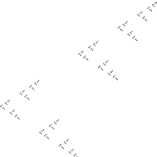
Figure 1. Graph of the fractal transformation $T_{FG_{1}}$ discussed in Example 3.3. This provides a Lebesgue measure-preserving transformation on [0,1] that is continuous a.e. but has a dense countable set of discontinuities. This transformation, and others like it, provide unitary transformations on $\mathcal{L}^{2}[0,1]$ and ”fractal Fourier series”, see Section 4. The viewing window is slightly larger than [0,1]$\times$[0,1].

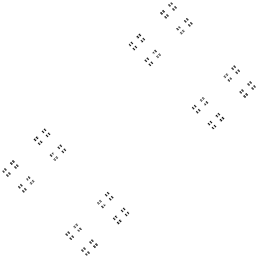
Figure 2. Graph of the fractal transformation $T_{FG_{2}}$ discussed in Section 3.3. Unlike $T_{FG_{1}}$ in Figure 1, $T_{FG_{2}}$ is its own inverse.

Example 3.4 (Hilbert’s space filling curve).

Space filling curves, from the point of view of IFS theory, have been considered in [24]. In [6] it is shown how, as follows, functions such as the Hilbert mapping $h:[0,1]\rightarrow$ $[0,1]^{2}$ (see Figure 3) are examples of fractal transformations.

Let $A=A_{1}=(0,0),B=B_{4}=(1,0),C=C_{3}=(1,1),D=D_{2}=(0,1),$ $B_{1}=A_{2}=(0,0.5),$ $C_{1}=B_{2}=A_{3}=D_{4}=(0.5,0.5),$ $D_{1}=C_{4}=(0.5,0),$ $C_{2}=D_{3}=(0.5,1),$ and $B_{3}=A_{4}=(1,0.5)$. Let

$$F =\left\{\mathbb{R};f_{i}=\frac{x+i-1}{4},i=1,2,3,4\right\},$$

$$G =\left\{\mathbb{R}^{2};g_{i},i=1,2,3,4\right\}$$

where $g_{i}:\mathbb{R}^{2}\rightarrow\mathbb{R}^{2}$ is the unique affine transformation such that $g_{i}(ABCD)=A_{i}B_{i}C_{i}D_{i}$, by which we mean $g_{i}(A)=A_{i}$, $g_{i}(B)=B_{i},g_{i}(C)=C_{i},g_{i}(D)=D_{i}$ for $i=1,2,3,4$. (Similar notation will be used elsewhere in this paper.) The Hilbert mapping is $h=T_{FG}:[0,1]\rightarrow[0,1]^{2},$ The functions in $G$ were chosen to conform to the orientations of Figure 3, which comes from Hilbert’s paper [16] concerning Peano curves. One way to prove that $T_{FG}$ is continuous is by using the standard theory of fractal transformations; see for example [6, Theorem 1].

If $p_{1}=p_{2}=p_{3}=p_{4}=0.25,$ then the associated invariant measure $\mu_{F}$ is the Lebesgue measure on $[0,1]$, and $\mu_{G}$ is Lebesgue measure on $[0,1]^{2}$. The inverse of $T_{FG}^{-1}$ is the fractal transformation $T_{GF}:[0,1]^{2}\rightarrow[0,1]$, which is continuous almost everywhere with respect to two dimensional Lebesgue measure. More precisely, $T_{GF}\circ h(x)=x$ for almost all $x\in[0,1]$ (with respect to Lebegue measure), and $h\circ T_{GF}(x)=x$ for all $x\in[0,1]^{2}$. By Theorem 2.4, the fractal transformation $h$ is Lebesque measure preserving in that the $2$-dimensional Lebesque measure of the image $h(B)$ of $B$ equals the $1$-dimensional Lebesque measure of $B$, for any Borel set $B$.

Figure 3. Hilbert’s original design for a continuous map from [0,1] to [0,1]$\times$[0,1].

Example 3.5 (Fractal transformations between the unit interval and a filled triangle).

Let $A,B,C$ be non-colinear points in $\mathbb{R}^{2}$ and let $D$ be the mid-point of the line segment $CA$. Let

$$F =\left\{\mathbb{R};f_{1}(x)=\frac{1}{2}\,x,\;f_{2}(x)=\frac{1}{2}\,x+\frac{1}{2}\,\right\},$$

$$G =\left\{\mathbb{R}^{2};g_{1},\;g_{2}\right\},$$

where $g_{1}$ and $g_{2}$ are the unique affine maps on $\mathbb{R}^{2}$ such that $g_{1}(ABC)=ADB$ and $g_{2}(ABC)=BDC$, respectively. The unique attractor of $F$ is $A_{F}=$ $[0,1]\subset\mathbb{R}$, and the unique attractor of $G$ is and $A_{G}=\triangle$, the filled triangle with vertices at $ABC$. If $p_{1}=p_{2}=0.5$ then $\mu_{F}$ is Lebesgue measure on $[0,1]$, and $\mu_{F}$ is Lebesgue measure on $\triangle$, It readily follows from [6, Theorem 1] that $T_{FG}:[0,1]\rightarrow\triangle$ is continuous and $T_{FG}([0,1])=\triangle$. It is also readily shown that $T_{GF}:\triangle\rightarrow[0,1]$ is continuous almost everywhere with respect to two-dimensional Lebesgue measure, with discontinuities located on a countable set of boundaries of triangles. We have that $T_{FG}\circ T_{GF}(x)=x$ for all $x\in\triangle$, and $T_{GF}\circ T_{FG}(x)=x$ for almost all $x\in[0,1],$ with respect to one-dimensional Lebesgue measure. We also have $T_{GF}(\triangle)\neq[0,1]$ but $\overline{T_{GF}(\triangle)}=[0,1]$.

Example 3.6 (A family of fractal homeomorphisms on a triangular laminar).

Let $\bigtriangleup$ denote a filled equilateral triangle as illustrated in Figure 4. The IFS $F_{r},\;0<r\leq\frac{1}{2},$ on $\bigtriangleup$ consists of the four affine functions as illustrated in the figure on the left, where $\bigtriangleup$ is mapped to the four smaller triangles so that points $A,B,C$ are mapped are mapped, respectively, to points $a,b,c$. A probability vector is associated with $F$ such that the probability is proportional to the area of the corresponding triangle. The IFS $G_{\lambda}$ is defined in exactly the same way, but according to the figure on the right. The attractor of each IFS is $\bigtriangleup$. (It is quite a subtle point, that there exists a metric, equivalent to the Euclidean metric on $\mathbb{R}^{2},$ such that both IFSs are contractive, see [Akins].) It is proved in [11] that the corresponding invariant measures $\mu_{F}$ and $\mu_{G}$ are both 2-dimensional Lebesque measure. By Theorem 2.4 and [6, Theorem 1], or by [11], the fractal transformation $T_{FG}^{r}$ is an area-preserving homeomorphism of $\bigtriangleup$ for all $0<r\leq\frac{1}{2}$. See [11] for related examples of volume-preserving fractal homeomorphisms between tetrahedra.

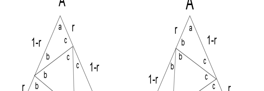
Figure 4. See Example 3.6.

4. Isometries between Hilbert Spaces

Given an IFS $F$ with attractor $A_{F}$ and an invariant measure $\mu_{F}$, the Hilbert space $L_{F}^{2}=L^{2}(A_{F},\mu_{F})$ of complex-valued functions on $A_{F}$ that are square integrable w.r.t. $\mu_{F}$ are endowed with the inner product $<\cdot,\cdot>_{F}$ defined by

$$\langle\psi_{F},\varphi_{F}\rangle_{F}=\int\limits_{A_{F}}\overline{\psi_{F}}\varphi_{F}\,d\mu_{F}\text{,}$$

for all $\psi_{F},\varphi_{F}\in L_{F}^{2}$. Functions that are equivalent, i.e., equal almost everywhere, will be considered the same function in $L_{F}^{2}$.

Definition 4.1.

Given two IFSs $F$ and $G$ with the same number of functions, with the same probabilities, with attractors $A_{F}$ and $A_{G}$ and invariant measures $\mu_{F}$ and $\mu_{G}$, respectively, let $T_{FG}$ and $T_{GF}$ be the fractal transformations. The induced isometries $U_{FG}:L_{F}^{2}\rightarrow L_{G}^{2}$ and $U_{GF}:L_{G}^{2}\rightarrow L_{F}^{2}$ are given by

$$(U_{FG}\varphi_{F})(y) =\varphi_{F}(T_{GF}(y))$$

$$(U_{GF}\varphi_{G})(x) =\varphi_{G}(T_{FG}(x))$$

for all $x\in A_{F}$ and all $y\in A_{G}$. That these linear operators are isometries is proved as part of Theorem 4.1 below.

Theorem 4.1.

Under the conditions of Definition 4.1,

1. $U_{FG}:L_{F}^{2}\rightarrow L_{G}^{2}$ and $U_{GF}:L_{G}^{2}\rightarrow L_{F}^{2}$ are isometries;

2. $U_{FG}\circ U_{GF}=id_{F}$ and $U_{GF}\circ U_{FG}=id_{G},$ the identity maps on $L_{F}^{2}$ and $L_{G}^{2}$ respectively;

3. $\langle\psi_{G},U_{FG}\varphi_{F}r\rangle_{G}\,=\,\langle U_{GF}\psi_{G},\varphi_{F}\rangle_{F}$ for all $\psi_{G}\in L_{G}^{2}$, $\varphi_{F}\in L_{F}^{2}$.

Proof.

(1) To show that the linear operators are isometries:

$$\left\|U_{FG}\varphi_{F}\right\|_{G}^{2} =\int_{A_{G}}|U_{FG}\varphi_{F}|^{2}d\mu_{G}$$

$$=\int_{A_{G}}|\varphi_{F}\circ T_{GF}|^{2}d\mu_{G}$$

$$=\int_{A_{F}}|\varphi_{F}|^{2}d(\mu_{G}\circ T_{FG})$$

$$=\int_{A_{F}}|\varphi_{F}|^{2}d\mu_{F}=\left\|\varphi_{F}\right\|_{F}^{2},$$

the third equality from the change of variable formula and Lemma 2.3; the fourth equality from statement (2) of Theorem 2.4.

(2) From the definition of the induced isometries

$$(U_{GF}\,U_{FG}(\varphi_{F}))(x)=\varphi_{F}(T_{GF}\,T_{FG}(x)).$$

But by Lemma 2.3, the fractal transformations $T_{GF}$ and $T_{FG}$ are inverses of each other almost everywhere. Therefore the functions $U_{GF}\,U_{FG}(\varphi_{F})$ and $\varphi_{F}$ are equal for almost all $x\in A_{F}$.

(3) This is an exercise in change of variables, similar to the proof of (1). ∎

Example 4.1 (The Cantor function).

Consider the two IFS’s $F=\{\mathcal{C};\,\frac{1}{3}x,\frac{1}{3}x+\frac{2}{3}\}$ and $G=\{[0,1];\,\frac{1}{2}x,\frac{1}{2}x+\frac{1}{2}\}$, the first with attractor equal to the standard Cantor set $\mathcal{C}$, the second with attractor equal to the unit interval. In this case the fractal transformation $T_{FG}:\mathcal{C}\rightarrow[0,1]$ is essentially the Cantor function. The Cantor function is usually defined as a function $f:[0,1]\rightarrow[0,1]$ so that if $x$ is expressed in ternary notation as $x=i_{1}\,i_{2}\,\cdots$ where $i_{k}\in\{0,1,2\}$ for all $k$, then $f(x)=i_{1}^{\prime}\,i_{2}^{\prime}\,\cdots$ expressed in binary, where $i^{\prime}=0$ if $i\in\{0,1\}$ and $i^{\prime}=1$ if $i=2.$ The function $T_{F,G}:\mathcal{C}\rightarrow[0,1]$ is essentially the same except the domain is $\mathcal{C}$ rather than $[0,1]$.

Let $F$ and $G$ be IFSs with the same probability vectors and corresponding invariant measures $\mu_{F}$ and $\mu_{G}$. If $\{e_{n}\}$ is an orthonormal basis for $L_{F}^{2}$, then by Theorem 4.1, the set $\{\widehat{e}_{n}\}=\{U_{FG}\,e_{n}\}$ is an orthonormal basis for $L_{G}^{2}$. In the following example, the two IFSs $F$ and $G$ have the same attractor $A_{F}=A_{G}=[0,1]$, and the invariant measures are both Lebesque measure. For example, the Fourier orthonormal basis $\{e^{2\pi inx}\}_{n=-\infty}^{\infty}$ of $L^{2}([0,1])$ is transformed under $U_{FG}$ to a “fractalized” orthonormal basis of $L^{2}([0,1])$. Therefore, to any function in $L^{2}([0,1])$ there is a Fourier series and also corresponding (via $T_{FG}$) a fractal Fourier series. (ii) To prove that $U_{FG}U_{GF}=I_{F}$ we remove from $A_{F}$ all point that have more than one address w.r.t. $F$, i.e. those point $x\in A_{F}$ for which $\pi_{F}^{-1}(x)$ is not a singleton and we also remove those points of $A_{F}$ for which $\pi_{G}^{-1}(T_{FG}(x))$ is not a singleton; this is the set $A_{F}^{G}$ defined earlier; it has full measure, and $T_{GF}T_{FG}|_{A_{F}^{G}}$ is the identity on $A_{F}^{G}$.

4.1. Fractal Fourier sine series

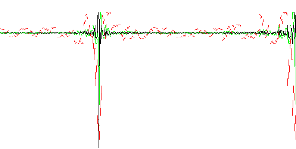
Figure 5. Fractal sine series approximations to a constant function on the interval $[0,1].$ The number of terms used here are $10$ (red), $50$ (green) and $100$ (black). Compare with Figure 6; the r.m.s. errors are the same as for the approximation to the same constant function using a sine series with the same number of terms. Notice that the edge effect has been shifted from $0$ to $1/3$.

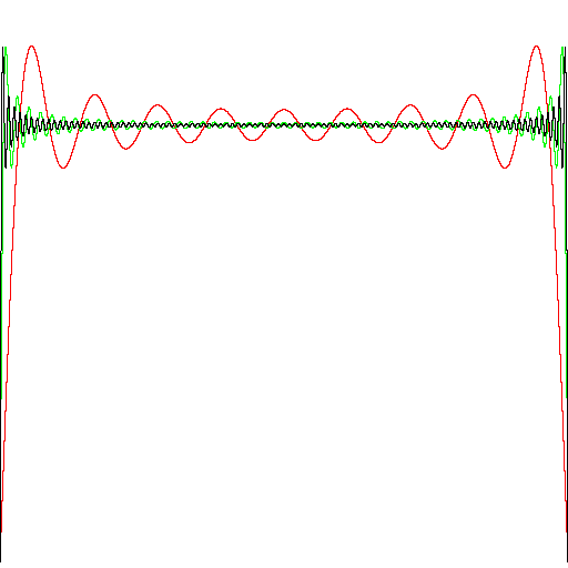
Figure 6. For comparison with Figure 5, this shows the Fourier sine series approximations to a constant function on $[0,1]$ using $k=10$ (red), $50$ (green) and $100$ (black) significant terms. Note the well-known end effects at the edges of the interval.

Consider the IFSs $F,G_{1},G_{2}$ of Example 3.3 with probabilities $p_{1}=p_{2}=0.5$. In this case $\mu_{F},\mu_{G_{1}}$ and $\mu_{G_{2}}$ are all Lebesque measure on $[0,1]$. Consider the orthonormal Fourier sine basis $\{\sqrt{2}\,e_{n}\}_{n=1}^{\infty}$ for $L^{2}[0,1]$, where $e_{n}=\sin(n\pi x)$.

For the fractal transformation $T_{FG_{1}},$ the fractally transformed orthonormal basis for $L^{2}[0,1]$ is $\{\sqrt{2}\,\widehat{e}_{n}\}_{n=1}^{\infty}$, where

$$\widehat{e}_{n}(x)=\sin(n\pi T_{G_{1}F}(x)),$$

for all $n\in\mathbb{N}$. Figure 7 illustrates ${\widehat{e}_{i}},\,i=1,2,3$, in colors black, red, and green, respectively. For comparison, Figure 8 illustrates the corresponding sine functions $\sin(n\pi x)$ for $n=1,2,3$.

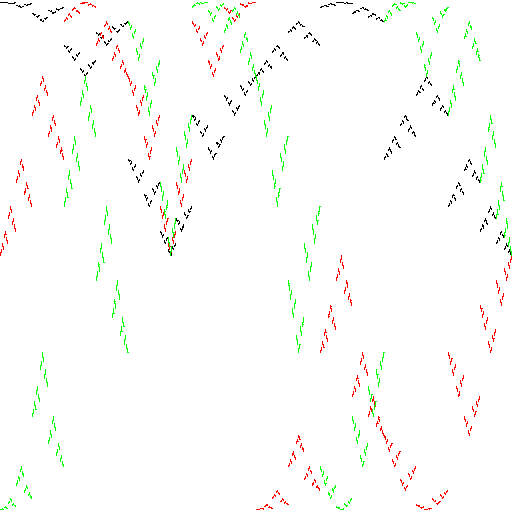
Figure 7. See text. The first three eigenfunctions of the elementary fractal transformed Laplacian on [0,1]; equivalently, the functions f-sin(n,x) for n=1 (black), 2 (red), 3 (green). The viewing window is [0,1]$\times$[-1,1].

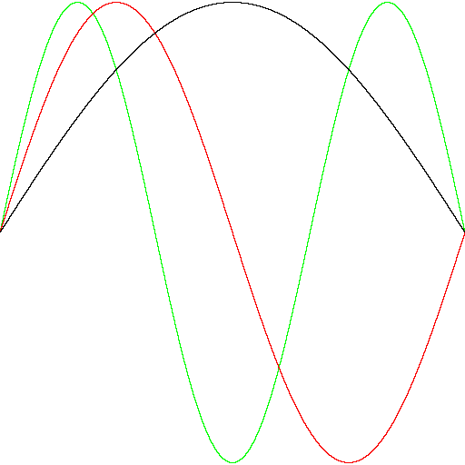
Figure 8. This illustrates the sine functions $sin(n\pi x)$ for n=1,2,3 for comparison with the fractal sine function shown in Figure 7.

Example 4.2 (Constant function).

Figure 5 illustrates three fractal Fourier sine series approximations to a constant function on the interval $[0,1]$, while Figure 6 illustrates the standard sine series Fourier approximation using the same numbers of terms. The respective Fourier series are

$$\sum_{n=1}^{\infty}\frac{\widehat{e}_{2n-1}(x)}{2n-1}\qquad\text{and}\qquad\sum_{n=1}^{\infty}\frac{e_{2n-1}\,(x)}{2n-1}.$$

The calculation, in the first case, of the Fourier coefficients, uses the change of variables formula, the fact from Example 3.3 that $\mu_{F}$ and $\mu_{G_{!}}$ are Lebesque measure, and statement 2 of Theorem 2.4. The mean square errors are the same when using the same number of terms.

Example 4.3 (Step function).

Next consider Fourier approximants to a step function. The fractal transformation $T_{FG_{2}}$ has fractal sine functions defined by

$$\widetilde{e}_{n}:=\sin(n\pi T_{G_{2}F}(x))$$

for all $n\in\mathbb{N}$. Figures 9, 10, and 11 illustrate the Fourier approximations for $100$ (green) and $500$ (black) terms, where the orthogonal bases functions are $e_{n},\;\widehat{e}_{n}$ and $\widetilde{e}_{n},$ respectively. The respective Fourier series are

$$\frac{2}{\pi}\,\sum_{n=1}^{\infty}\frac{1-\cos(n\pi/2)}{n}\,f_{n}(x),$$

where $f_{n}$ is $e_{n},\;\widehat{e}_{n}$ and $\widetilde{e}_{n},$ respectively. The point to notice is that the jump in the step function at $x=0.5$ is cleanly approximated in both the fractal series, in contrast to the well-known edge effect (Gibbs phenomenon) in the classical case. The price that is paid is that the fractal approximants have greater pointwise errors at some other values of $x$ in $[0,1]$. The analysis of where this occurs and proof that the mean square error is the same for all three schemes, is omitted here.

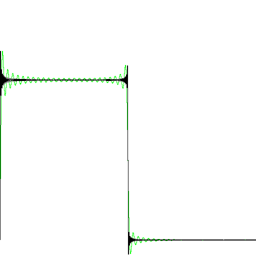
Figure 9. Sum of the first 100 (green) and 500 (black) terms in the Fourier sine series for a step function. The viewing window is [0,1]$\times$[-0.1,1.5]. Compare with Figures 10 and 11.

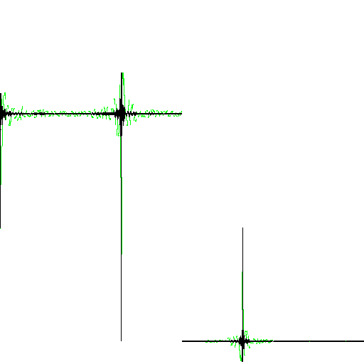
Figure 10. Sum of the first 100 (green) and 500 (black) terms in a fractal Fourier sine series (using f-sin(n,x) functions) for a step function. Compare with Figures 9 and 11.

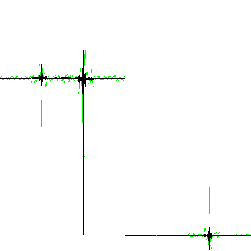
Figure 11. Sum of the first 100 (green) and 500 (black) terms in a fractal Fourier sine series (using f2-sin(n,x) functions) for a step function. Compare with Figures 9 and 10.

Example 4.4 (Tent function).

In Figure 12 partial sums of the Fourier sine series and their fractal counterparts are compared, for the tent function $f(x)=\min\{x,1-x\}$ on the unit interval. The Fourier series with orthogonal functions $e_{n}$ is compared with the Fourier series with fractal orthogonal functions $\widetilde{e}_{n}$, using $3$ (red), $5$ (green), $7$ (blue), $20$ (black) terms. The Fourier series are (up to a normalization constant)

$$\sum_{n=1}^{k}\frac{2\sin(\pi n/2)-\sin(\pi n)}{n^{2}}\,e_{n}(x)\ \qquad\text{ and }\qquad\sum_{n=1}^{k}\frac{2\sin(\pi n/2)-\sin(\pi n)}{n^{2}}\,\widetilde{e}_{n}(x).$$

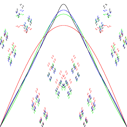
Figure 12. See Example 4.4. Fourier sine series approximants to a tent function and fractal counterparts.

Example 4.5 (Function with a dense set of discontinuities).

Consider the following approximation of a function with a dense set of discontinuities. For $i=1,2$, let $\psi\in L^{2}[0,1]$ be defined by $\psi(x)=x$ for all $x\in[0,1]$. Then $\phi_{i}=U_{FG_{i}}\psi,\,i=1,2,$ is given by $\phi_{i}(x)=(U_{FG_{i}}\psi)(x)=\psi(T_{G_{i}F}(x))=T_{G_{i}F}(x)$, which has a dense set of discontinuities. It follows, by a short calculaltion using statement 2 of Theorem 2.4, that the coefficients in the $\widehat{e}_{n}$ and $\widetilde{e}_{n}$ Fourier series expansion of $\phi_{i}$ are the same as the coefficients in the $e_{n}$ expansion for $\psi$. Therefore the fractal version Fourier series expansions for $\phi_{i},\,i=1,2,$ are

$$\frac{2}{\pi}\sum_{n=1}^{\infty}\frac{-\cos(\pi n)}{n}\;\widehat{e}_{n}(x),\qquad\text{and}\qquad\frac{2}{\pi}\sum_{n=1}^{k}\frac{-\cos(\pi n)}{n}\,\widetilde{e}_{n}(x),$$

respectively. Sums with $10,30,$ and $100$ terms are shown in red, green, and blue, respectively, in Figure 13 for $\phi_{1}$, and for $\phi_{2}$ in Figure 14 using the first 1000 terms of the series.

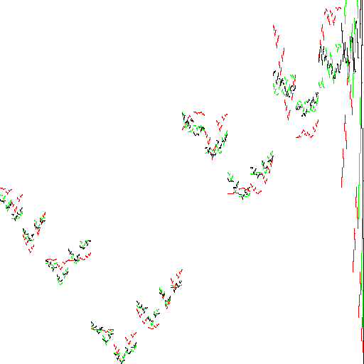
Figure 13. See Example 4.5. Compare with Figure 1. The approximants converge to $T_{G_{1}F}(x)$ in $\mathcal{L}^{2}[0,1]$ as the number of terms in series sum approaches infinity.

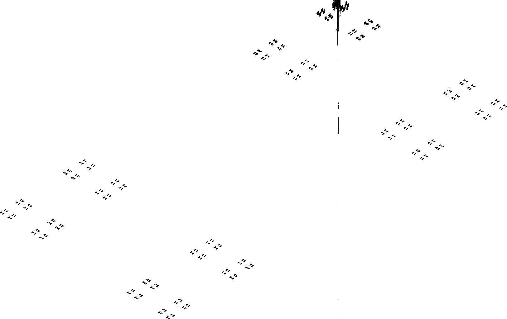
Figure 14. See Example 4.5. This illustrates the sum of the first thousand terms of a fractal sine series for $T_{FG_{2}}(x)$ on $[0,1]$. Compare with Figure 2.

4.2. Legendre polynomials.

The Legendre polynomials are the result of applying Gram-Schmidt orthogonalization $\{1,x,x^{2},\dots\}$, with respect to Lebesgue measure on $[-1,1]$. Denote the Legendre polynomials shifted to the interval $[0,1]$ by $\{P_{n}(x)\}_{n=0}^{\infty}$. They form a complete orthogonal basis for $L^{2}[0,1]$, where the inner product is

$$\langle\psi,\varphi\rangle\,=\int\limits_{0}^{1}\overline{\psi(x)}\varphi(x)dx\text{.}$$

In this case each of the unitary transformations $U_{FG}$ associated with Example 3.3 maps $L^{2}[0,1]$ to itself, and we obtain the “fractal Legendre polynomials”

$$P_{n}^{FG}(x)=P_{n}(T_{GF}(x))\text{.}$$

With $F,G_{1},G_{2}$ as previously defined in Example 3.3, Figures 15 and 16 illustrate the Legendre polynomials and their fractal counterparts. Figure 15 shows the fractal Legendre polynomials $P_{n}^{FG_{1}}(x)$ and Figures 16 shows the fractal Legendre polynomials $P_{n}^{FG_{2}}(x)$.

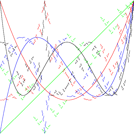
Figure 15. Legendre polynomials and their fractal counterparts corresponding to $T_{FG_{1}}$. Both sets of functions form orthogonal basis sets with respect to Lebesgue measure on the interval $[-1,1]$. See also Figure LABEL:Legendref2.

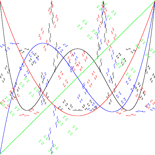
Figure 16. Legendre polynomials and their fractal counterparts corresponding to $T_{FG_{2}}$. See also Figure 15.

4.3. The action of the unitary operator on Haar wavelets.

With $F,G_{2}$ and $T=T_{FG_{2}}:\mathbb{[}0,1]\rightarrow[0,1]$ as previously defined, let $U=U_{FG_{2}}:L^{2}[0,1]\rightarrow L^{2}[0,1]$ be the associated (self-adjoint) unitary transformation. Let $I_{\emptyset}=[0,1]$ and $H_{\emptyset}:\mathbb{R}\rightarrow\mathbb{R}$ be the Haar mother wavelet defined by

$$H_{\emptyset}(x)=\left\{\begin{array}[c]{c}+1\text{ if }x\in[0,0.5)\text{,}\\ -1\text{ if }x\in[0.5,1)\text{,}\\ 0\text{ otherwise.}\end{array}\right.$$

For $\sigma\in\{0,1\}^{k},\,k\in\mathbb{N}$, write $\sigma=\sigma_{1}\sigma_{2}...\sigma_{k}$ and $\left|\sigma\right|=k$. If $\left|\sigma\right|=0$ then $\sigma=\emptyset$, the empty string. Also let $I_{\sigma}=h_{\sigma_{1}}\circ h_{\sigma_{2}}\circ...\circ h_{\sigma_{k}}(I_{\emptyset}),$ where $h_{0}=f_{1}$ and $h_{1}=f_{2}$, and let $A_{\sigma}:\mathbb{R\rightarrow R}$ be the unique affine map such that $A_{\sigma}(I_{\emptyset})=I_{\sigma}$. With this notation, the standard Haar basis, a complete orthonormal basis for $L^{2}[0,1]$, is

$$\{H_{\sigma}:\sigma\in\{0,1\}^{k},k\in\mathbb{N\}\cup\{}H_{\emptyset}(x)\}\cup\{\mathbf{1}\},$$

where $\mathbf{1}$ is the characteristic function of $[0,1)$ and $H_{\sigma}:[0,1)\rightarrow\mathbb{R}$ is defined by

$$H_{\sigma}(x)=2^{\left|\sigma\right|/2}H_{{}_{\emptyset}}(A_{\sigma}^{-1}(x))\text{.}$$

There is an interesting action of $U=U_{FG_{2}}$ on Haar wavelets. The operator $U$ permutes pairs of Haar wavelets at each level and flips signs of those at odd levels, as follows. By calculation, for $\sigma\in\cup_{k\in\mathbb{N}}\{0,1\}^{k}$,

$$UH_{\sigma}=(-1)^{\left|\sigma\right|}H_{\sigma^{\prime}}$$

where $\left|\sigma\right|=\left|\sigma^{\prime}\right|$ and $\sigma_{l}^{\prime}=(-1)^{l+1}\sigma_{l}+(1+(-1)^{k})/2$ for all $l=1,2,...,\left|\sigma^{\prime}\right|$, $UH_{\emptyset}=H_{\emptyset}$, and $U1=1$. It follows that if $f\in L^{2}[0,1]$ is of the special form

$$f=a_{\emptyset}H_{\emptyset}+\sum_{\sigma\in\cup_{k\in\mathbb{N}}\{0,1\}^{2k}}c_{\sigma}(H_{\sigma}+H_{\sigma^{\prime}})\text{,}$$

then $Uf=f$ and $f\circ T=f$. Such signals are invariant under $U$. It also follows that if $P$ is the projection operator that maps $L^{2}[0,1]$ onto the span of all Haar wavelets down to a fixed depth, then $U^{-1}PU=P$.

4.4. Unitary transformations from the Hilbert mapping and its inverse

This continues Example 3.4, where the fractal transformations $h:=T_{FG}$ and $h^{-1}:=T_{GF}$ are the Hilbert mapping and its inverse, both of which both preserve Lebesgue measure and are mappings between one and two dimensions. The unitary transformations $U_{FG}\,:\,L^{2}([0,1])\rightarrow L^{2}([0,1]^{2})$ and $U_{GF}\,:\,L^{2}([0,1]^{2})\rightarrow L^{2}([0,1])$ are given by

$$U_{FG}(f)=f\circ h^{-1},\qquad\qquad U_{GF}(f)=f\circ h.$$

A picture can be considered as a function $f:[0,1]^{2}\rightarrow\mathbb{R}^{3}$, where the image of a point $x$ in ${\mathbb{R}}^{3}$ gives the RGB colours. The top image of Figure 17 is a picture of the graph of such a function $f:[0,1]^{2}\rightarrow\mathbb{R}^{3}$. The bottom image is the function (picture) $U_{GF}f=f\circ h$ transformed by the unitary operator.

Figure 17. See Section 4.4.

The Hilbert map $h:[0,1]\rightarrow[0,1]^{2}$ is continuous, one consequence of which is that, if $f:[0,1]^{2}\rightarrow\mathbb{R}^{3}$ is continuous, then so is the pull-back $U_{GF}(f)=f\circ h:[0,1]\rightarrow\mathbb{R}^{3}$. To illustrate, any orthonormal basis w.r.t. Lebesgue measure on $[0,1]$ is mapped, via the unitary operator $U_{FG}$, to an orthonormal basis w.r.t. Lebesgue measure on $[0,1]^{2}$, and conversely. Because the Hilbert mapping is continuous, an orthonormal basis of continuous functions $\{\psi_{n}:[0,1]^{2}\rightarrow$ $\mathbb{R\}}$ is transformed by $U_{GF}$ to an orthonormal basis of continuous functions $\{\psi_{n}\circ h:[0,1]\rightarrow$ $\mathbb{R\}}$. In the other direction, the image of an orthonormal basis consisting of continuous functions on $[0.1]$ may not comprise continuous functions on $[0,1]^{2}$. Figures 18 and 19 illustrate this.

In Figure 20, the right image represents the graph of $f:[0,1]^{2}\rightarrow[-1,1]$ defined by $f(x,y)=\sin(\pi x)\sin(\pi y)$. The left image represents the graph of $g:[0,1]^{2}\rightarrow[-1,1]$ defined by the continuous function $g(x,y)=U_{GF}(f)=f\circ h(x)$ where $h:[0,1]\rightarrow[0,1]^{2}$ is the Hilbert function. The set of functions in the orthogonal basis $\left\{\sin(n\pi x)\sin(m\pi y):n,m\in\mathbb{N}\right\}$ for $L^{2}([0,1]^{2})$ (w.r.t.Lebesque two-dimensional measure) is fractally transformed via the Hilbert mapping to an othogonal basis for $L^{2}[0,1]$ (w.r.t.Lebesgue one-dimensional measure). In contrast to the situation in Section 4.1, these ”fractal sine functions” are continuous.

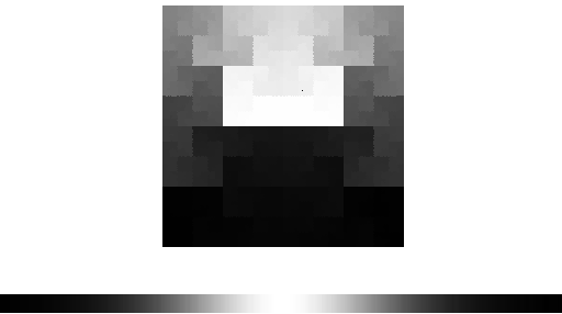
Figure 18. The bottom band shows the graph of $\sin(\pi x)$ with function values represented by shades of grey. The top band shows the graph of $h(sin(\pi x))$, where $h$ is the Hilbert function.

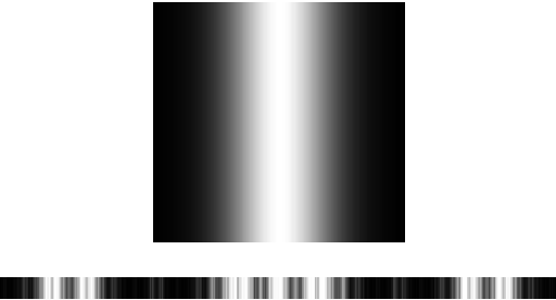
Figure 19. The top image illustrates the graph of $f(x,y)=\sin(\pi x)$ for $x,y\in[0,1]^{2}$. The band at the bottom illustrates the graph of the pull-back $f\circ h:[0,1]\rightarrow[-1,1]$, which is continuous, in contrast to the situations in Figures 17.

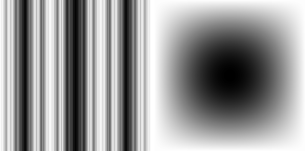
Figure 20. The right image represents the graph of $f:[0,1]^{2}\rightarrow[-1,1]$ defined by $f(x,y)=\sin(\pi x)\sin(\pi y)$. The left image represents the graph of $g:[0,1]^{2}\rightarrow[-1,1]$ defined by the continuous function $g(x,y)=U_{GF}(f)=f\circ h(x)$ where $h:[0,1]\rightarrow[0,1]^{2}$ is the Hilbert function.

5. Fractal Transformation of a Linear Operator

Let $F$ and $G$ be IFSs with the same number of functions. Using the same notation as in the previous section, if $W_{F}\,:\,L^{2}_{F}\rightarrow L^{2}_{F}$ is a linear operator, then the fractally transformed linear operator $W_{G}:\,L^{2}_{G}\rightarrow L^{2}_{G}$ defined by

$$W_{G}=U_{FG}\circ W_{F}\circ U_{GF}$$

is also a linear operator. If $W_{F}$ is a bounded, self-adjoint linear ooperator with spectral representation

$$W_{F}=\int_{-\infty}^{+\infty}\lambda dP_{\lambda}^{F}\text{,}$$

where $P_{\lambda}^{F}$ is an increasing family of projections on $L_{F}^{2}$, then

$$W_{G}=\int_{-\infty}^{+\infty}\lambda dP_{\lambda}^{G}$$

where $P_{\lambda}^{G}=U_{FG}\circ P_{\lambda}^{F}\circ U_{GF}$. In particular, $W_{F}$ and $W_{G}$ have the same spectrum.

5.1. Differentiable functions

Definition 5.1.

Let $F$ and $G$ be IFSs with $F$ and $G$ non-overlapping, and $T_{FG}$ the fractal transformation from $A_{F}$ to $A_{G}$. Assume that the attractor $A_{F}$ of $F$ is the interval $[0,1]$, and denote the $k$ times continuously differentiable functions $f:A_{F}=[0,1]\rightarrow{\mathbb{R}}$ by $C_{F}^{k}$. The set

$$C_{G}^{k}=\{U_{FG}f\,:\,f\in C_{F}^{k}\}$$

will be called $k$ times continuously differentiable fractal functions. If the $k^{th}$ derivative of $f\in C_{F}^{k}$ is denoted $D_{F}^{k}\,f$, where $D_{F}^{k}$ is the differential operator, then

$$D_{G}^{k}\,g:=(U_{FG}\circ D_{F}^{k}\circ U_{GF})\,g$$

will be referred to as the $k^{th}$ fractal derivative of $g\in C_{G}^{k}$.

Note that analogous definitions can be made when $A_{F}$ is a subset of ${\mathbb{R}}^{n}$ with nonempty connected interior, for example a square or filled triangle in the plane. In that case, we have partial derivatives.

To obtain an intuitive interpretation of the fractal derivative, consider the case where the attractor of $F$ (with probability vector $p$) is $[0,1]$ as above and $F$ has the property that $\pi_{F}$ is an increasing function from the code space to $[0,1]$ with respect to the lexicographic order on the code space. Assume, similarly, that $G$ (with the same probability vector $p$) has the property that there is a linear order $\preceq$ on $A_{G}$ such that $\pi$ is increasing with respect to this order on $A_{G}$ and the lexicographic order on the code space. Assume further that $T_{FG}$ is a fractal homeomorphism. Note that all the above assumptions hold in Examples 4.1 of the Cantor set and Example 3.3 of the Koch curve.

For $y_{1},y_{2}\in A_{G}$ we use the following notation for the interval: $[y_{1},y_{2}]=\{y\,:\,y_{1}\preceq y\preceq y_{2}\}$. Under these assumptions, and with Lebesque measure $\mu$ as the invariant measure of $F$ and $\mu_{G}$ the invariant measure of $G$, define the fractal difference betwen a pair of points in $A_{G}$ by

$$y_{1}-y_{2}=\begin{cases}\mu_{G}([y_{2},y_{1}])\qquad\text{ if }\;y_{1}\geq y_{2},\\ -\mu_{G}([y_{1},y_{2}])\quad\text{ if }\;y_{1}<y_{2}.\end{cases}$$

Theorem 5.1.

With notation as above, if $g:A_{G}\rightarrow{\mathbb{R}}$ is a differentiable fractal function, then

$$D_{G}\,g\,(y_{0})=\lim_{y\rightarrow y_{0}}\frac{g(y)-g(y_{0})}{y-y_{0}}.$$

Proof.

If $g:A_{G}\rightarrow{\mathbb{R}}$ is a differentiable fractal function, then there is an $f:[0,1]\rightarrow{\mathbb{R}}$ such that $g=U_{FG}\,f$. Now

$$D_{G}\,g(y_{0}) =(U_{FG}\circ\frac{d}{dx}\circ U_{GF}\,g)\,(y_{0})=((U_{FG}\circ\frac{d}{dx}\circ U_{GF})\,(U_{FG}\,f))\,(y_{0})$$

$$=((U_{FG}\circ\frac{d}{dx})\,f)(y_{0})=(U_{FG}\circ f^{\prime})\,(y)=f^{\prime}(T_{GF}\,y_{0})=\lim_{x\rightarrow T_{GF}\,y_{0}}\frac{f(x)-f(T_{GF}\,y_{0})}{x-T_{GF}\,y_{0}}.$$

Given $x\in[0,1]$, there is a unique $y_{x}\in A_{G}$ such that $T_{GF}\,y_{x}=x$. Moreover, since $T_{GF}$ is continuous, as $y\rightarrow y_{0}$ we have $T_{GF}\,y\rightarrow T_{GF}\,y_{0}$, i.e., $x\rightarrow T_{GF}\,y_{0}$. Therefore

$$D_{G}\,g(y_{0})=\lim_{y\rightarrow y_{0}}\frac{f(T_{GF}\,y)-f(T_{GF}\,y_{0})}{T_{GF}\,y-T_{GF}\,y_{0}}=\lim_{y\rightarrow y_{0}}\frac{g(y)-g(y_{0})}{T_{GF}\,y-T_{GF}\,y_{0}}.$$

By Lemma 2.2, if $\nu$ is the invariant measure on code space with probability vector $p$, then (assume $y\succeq y_{0}$ without loss of generality)

$$\mu([T_{GF}\,y_{0},T_{GF}\,y]) =\nu(\pi_{F}^{-1}([T_{GF}\,y_{0},T_{GF}\,y])=\nu([\pi_{F}^{-1}\,T_{GF}\,y_{0},\pi_{F}^{-1}\,T_{GF}\,y])$$

$$=\nu([\tau_{G}\,y_{0},\tau_{G}\,y])=\nu([\pi_{G}^{-1}\,y_{0},\pi_{G}^{-1}\,y])=\nu(\pi_{G}^{-1}([y_{0},y]))$$

$$=\mu_{G}([y_{0},y])=y-y_{0}.$$

Therefore

$$D_{G}\,g\,(y_{0})=\lim_{y\rightarrow y_{0}}\frac{g(y)-g(y_{0})}{y-y_{0}}.$$

∎

Example 5.1 (Derivative of the Cantor function).

Consider the two IFS’s $F=\{[0,1];\,\frac{1}{2}x,\frac{1}{2}x+\frac{1}{2}\}$ and $G=\{\mathcal{C};\,\frac{1}{3}x,\frac{1}{3}x+\frac{2}{3}\}$ of Example 4.1. Let $T_{FG}:[0,1]\rightarrow\mathcal{C}$ be the fractal transformation from the unit interval to the Cantor set. If $f:[0,1]\rightarrow{\mathbb{R}}$ is the function $f(x)=x$, for example, then $g:=U_{FG}\,f=T_{GF}$ is exactly the Cantor function described in Example 4.1. The fractal derivative of this Cantor function $g$ is

$$(D_{G}\,g)(y)=(U_{FG}\circ D_{F}\circ U_{GF}\,g)(y)=(U_{FG}\circ D_{F}\circ U_{GF}\circ U_{FG}\,f)(y)=(U_{FG}\circ\mathbf{1}_{F})(y)=\mathbf{1}_{G}(y)=1$$

for all $y\in\mathcal{C}$, where $\mathbf{1}_{F}$ and $\mathbf{1}_{G}$ are the constant $1$ functions on $[0,1]$ and $\mathcal{C}$, respectively. Therefore the Cantor function has constant a.e. fractal derivative $1$.

Since the fractal transformation $T_{FG}$ induces transformations on the set of points of $A_{F}$, on the set $L_{2}(F)$ of functions on $A_{F}$, and on the set of linear operators on $L^{2}(F)$, any differential equation on $A_{F}$ can be transformed into a differential equation on $A_{G}$.

Example 5.2 (Differential equation on the Koch curve).

Consider the fractal transformation of Example 3.3, from the unit interval to the Koch curve. The simple initial value ODE

$$\frac{dy}{dx}=y,\quad y(0)=1$$

on the interval $[0,1]$ with solution $y=e^{x}$ transforms to the fractal ODE

$$(U_{FG}\circ\frac{d}{dx}\circ U_{GF})\,\widehat{y}=\widehat{y},\qquad\widehat{y}(T_{FG}0)=1$$

on the Koch curve. The fractal solution to this ODE is the function $g:=U_{FG}(\exp)$, i.e., $g(x)=e^{T_{GF}(x)}$.

6. Fractal Flows

Let $(X,\mu)$ be a metric space with Borel measure $\mu$, and let $f:X\rightarrow X$ be invertible almost everywhere, i.e. if there is a function $f^{-1}:X\rightarrow X$ such that $f\circ f^{-1}(x)=f^{-1}\circ f(x)-x$ for all $x$ in a set of measure $1$. Let ${\mathcal{M}}(X)$ be the set of Borel measures on $X$. Slightly abusing notation, we use the same symbol $f^{\#}$ for the following induced actions on $L^{2}(X)$ and ${\mathcal{M}}(X)$, respectively:

$$f^{\#}(\phi) =\phi\circ f^{-1}\quad\text{for}\;\phi\in L^{2}(X)$$

$$f^{\#}(\mu) =\mu\circ f^{-1}\quad\text{for}\;\mu\in{\mathcal{M}}(X).$$

Let $F$ be an IFS on the space $X$, $G$ an IFS on the space $Y$, and $T_{FG}\,:\,X\rightarrow Y$ a fractal transformation. Let $\mu_{F}$ and $\mu_{G}$ be the corresponding invariant measures with respect to the same probability vector. If $f:X\rightarrow X$ is invertible a.e., then define induced actions on $Y,L^{2}(Y),$ and ${\mathcal{M}}(Y)$ as follows. Again we use the same notation ${\widehat{f}}^{\#}$ for the induced actions, where $y\in Y,\phi\in L^{2}(Y)$, and $\mu\in{\mathcal{M}}(Y)$:

$$g(y):= {\widehat{f}}^{\#}(y)=T_{FG}\circ f\circ T_{GF}(y)$$

$${\widehat{f}}^{\#}(\phi)=g^{\#}(\phi)=U_{FG}\circ f^{\#}\circ U_{GF}(\phi)$$

$${\widehat{f}}^{\#}(\mu)=g^{\#}(\mu).$$

Note that, if $f$ is measure preserving on $X$, then by Theorem 2.4 the induced function $g$ is measure preserving on $Y$.

By a flow on a space $X$ is meant a mapping $f\,:\,X\times{\mathbb{R}}\rightarrow X$, with notation $f_{t}(x)$ often used instead of $f(x,t)$, such that

$$f_{0}(x)=x$$

$$f_{s}(f_{t}(x))=f_{s+t}(x)$$

for all $x\in X$ and all $s,t\in{\mathbb{R}}$. Applying the induced actions defined above to each function $f_{t},\,t\in{\mathbb{R}}$, motivates the following notion of fractal flows. Note that there are fractal flows on the metric space $Y$, and the space of square integrable functions $L^{2}(Y)$ and on the space of measures ${\mathcal{M}}(Y)$.

Definition 6.1.

A flow $f_{t}$ on $X$ induces flows $(f_{t})^{\#}$ on $L^{2}(X)$ and ${\mathcal{M}}(X)$, and, given a fractal transformation $T_{FG}$, the flow $f_{t}$ induces fractal flows $(\widehat{f_{t}})^{\#}$ on $Y,L^{2}(Y),$ and ${\mathcal{M}}(Y)$. Since, for a flow, $f_{t}^{-1}=f_{-t}$, the explicit formulas for the flows are

$$g_{t}(y):= {\widehat{f}_{t}}^{\#}(y)=T_{FG}\circ f_{t}\circ T_{GF}(y)$$

$${\widehat{f}_{t}}^{\#}(\phi)=g_{t}^{\#}(\phi)=U_{FG}\circ f_{t}y^{\#}\circ U_{GF}(\phi)$$

$${\widehat{f}}_{t}^{\#}(\mu)=g_{t}^{\#}(\mu).$$

If $f_{t}$ is a continuous, measure preserving flow on $(X,\mu)$, then it is readily checked that the flow $f_{t}^{\#}:L^{2}(X)\rightarrow L^{2}(X)$ is unitary, and hence provides a strongly continuous one parameter unitary group. By Stone’s theorem [27] there is a unique self-adjoint operator $L$ such that

$$f_{t}^{\#}=e^{itL},$$

where $iL$ is referred to as the infinitesimal generator. Moreover, ${\widehat{f}}_{t}^{\#}=U_{FG}\circ f_{t}^{\#}\circ U_{GF}:L^{2}(Y)\rightarrow L^{2}(Y)$ is a fractal flow with infinitesimal generator $i\widehat{L}=U_{FG}\circ L\circ U_{GF}$.

Example 6.1 (Vector field flow).

Let $V:{\mathbb{R}}^{2}\rightarrow{\mathbb{R}}^{2}$ be a 2-dimensional vector field given by $V(x,y)=(-y,x)$. Define a flow $f:{\mathbb{R}}^{2}\times{\mathbb{R}}\rightarrow{\mathbb{R}}^{2}$, in the usual way by solving the autonomous system

$$\frac{d}{dt}f(\mathbf{a},t)=V(f(\mathbf{a},t)),\qquad f(\mathbf{a},0)=\mathbf{a}.$$

The solution is, with notation $f_{t}(\mathbf{a})=f(\mathbf{a},t)$ and $\mathbf{a}=(a,b)$,

$$f_{t}(a,b)=(a\,\cos t+b\,\sin t,\;a\,\sin t-b\,\cos t).$$

With $a,b$ fixed, as a function of $t$, the flow curves are circles centered at the origin, so the domain of the flow $f_{t}(\mathbf{a})$ can be restricted to $D\times{\mathbb{R}}$, where $D$ is the closed unit disk.

Now consider the area preserving fractal homeomorphism of Example 3.6. Let $D$ be the largest inscribed disk in the equilateral triangle $\bigtriangleup$. Without loss of generality, assume that $D$ has radius $1$ and consider the flow $f_{t}(\mathbf{x})$ as in the paragraph above. The fractally transformed flow, as in Definition 6.1, is

$$g_{t}(\mathbf{y})=T_{FG}\circ f_{t}\circ T_{GF}\,(\mathbf{y}),$$

which as a function of $\mathbf{y}$, is area preserving. If the fractally transformed vector field is denoted $\widehat{V}=T_{FG}\circ V\circ T_{GF}$, then $g_{t}$ is the fractal flow of the vector field $\widehat{V}$. See Figure 21.

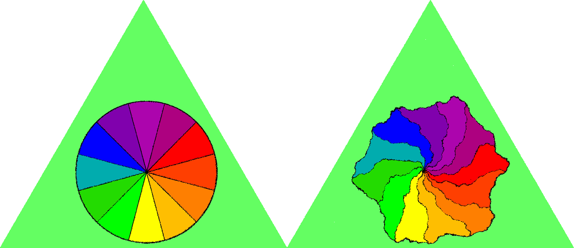
Figure 21. This image relates to Example 21.

Example 6.2 (Fractal flows on the unit interval and the circle).

Consider the Lebesgue measure preserving flow on a line segment $[0,1]$ or the circle $S^{1}$ defined by $f_{t}:[0,1]\rightarrow[0,1],$ $t\in(-\infty,\infty),$ defined by

$$x\mapsto(x+t)\operatorname{mod}1\text{.}$$

Consider any measure $\rho$ supported on $[0,1]$ that is absolutely continuous with respect to Lebesque measure $\mu$. We may treat $\rho$ as a model for the brightness and colours of a one-dimensional picture: the rate at which light of a set of frequencies is emitted, or reflected, in unit time under steady illumination by the Borel set $B$ is $\rho_{0}(B)$; see [5]. A vector of measures $(\rho_{R},\rho_{G},\rho_{B})$ represents the red, green, and blue components. With notation as above, $f_{t}^{\#}:\mathcal{M}\rightarrow\mathcal{M}$ is a flow on $\mathcal{M}$. The orbit of a particular measure $\rho_{0}$ models the picture being transported/translated at constant velocity along the line segment (what comes out at one end of the line segment immediately reenters the other end) or around the circle $S^{1}$.

Given an initial measure $\rho_{0}$, absolutely continuous with respect to Lebesque measure, consider its orbit $\rho_{t}=f_{t}^{\#}(\rho_{0})$, i.e. $\rho_{t}(B)=\rho_{0}(f_{-t}B)$. Interpreted in the model, $\rho_{t}$ is the translated picture/measure. By the Radon Nikodym theorem there is a measurable function $\varrho_{0}$ such that

$$\rho_{0}(B)=\int\limits_{B}\varrho_{0}(x)\,d\mu=\langle\chi_{B},\varrho_{0}\rangle$$

for all Borel sets $B$, where $\chi_{B}$ is the indicator function for $B$. It follows that

$$\rho_{t}(B)=\int\limits_{B}\varrho_{t}(x)\,d\mu\,=\,\langle\chi_{B},\varrho_{t}\rangle\,=\,\langle f_{t}^{\#}\chi_{B},\varrho_{0}\rangle,$$

where $\varrho_{t}(x)=f_{-t}^{\#}(\varrho_{0})(x)=\varrho_{0}((x+t)\mod 1)$, and the last equality by a change of variable. Letting $V_{t}:=f_{t}^{\#}:L^{2}(S^{1})\rightarrow L^{2}(S^{1})$ , by the comments prior to this example, $f_{t}^{\#}=e^{itL}$, where $L$ is a self-adjoint operator. It is well-known that, for this choice of the flow $f_{t}$, the operatort $L$ is an extension of the differential operator $-i\frac{d}{dx}$ acting on infinitely differentiable functions on $S^{1}$. Therefore, on an appropriate domain,

$$V_{t}=e^{itL}=e^{t\frac{d}{dx}}.$$

Let $T_{FG}:[0,1]\rightarrow[0,1]$ be a uniform Lebesgue measure-preserving fractal transformation, as considered in Section 4.1, and let $U_{FG}:L^{2}([0,1])\rightarrow L^{2}([0,1])$ be the corresponding unitary transformation. Then the fractal flow

$$\widehat{V}_{t}:={\widehat{f}}_{t}^{\#}=U_{FG}\,V_{t}\,U_{GF}$$

is again a strongly continuous one parameter unitary group generated by the self-adjoint operator $\widetilde{L}:=U_{FG\,}L\,U_{GF}$.

Figure 22 illustrates a fractal flow on $[0,1]$ for the case of $T_{FG_{1}}$ in Example 3.3 and Section 4.1. The bottom strip shows an initial function $\varphi$ on the interval $[0,1]$. In its orbit $V_{t}(\varphi),\,t\geq 0$, this picture slides to the right, colours going off the right-hand end and coming on at the left end, cyclically (not in the figure). From the top of the figure reading downwards, the successive strips show the same orbit under the fractal flow ${\widehat{V}}_{t}$ at times $t=0,1,2,...,7$. Then there is a white gap, followed by the flow at time $t=100$.

A surprising property of the flow orbit $\rho_{t}$ is that it is a continuous function of $t$, although $U_{FG}$ may map continuous functions to discontinuous ones. The proof is a consequence of the fact [26, Proposition 2.5] that $\|f_{t}^{\#}\varrho-\varrho\|_{L^{1}}\rightarrow 0$ as $t\rightarrow 0$.

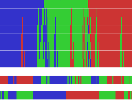
Figure 22. See text. Illustration of a fractal flow.

References

- [1] R. Atkins, M. F. Barnsley, A. Vince, D. Wilson, A characterization of hyperbolic affine iterated function systems, Topology Proceedings 36 (2010) 189-211.
- [2] C. Bandt, S. Graf, Self-similar sets 7. A characterization of self-similar fractals with positive Hausdorff measure, Proc. Am. Math. Soc. 114 (1992) 995-1001.
- [3] M. F. Barnsley, Fractal functions and interpolation, Constr. Approx. 2 (1986) 303-329
- [4] M. F. Barnsley, Theory and applications of fractal tops, in Fractals in Engineering: New Trends in Theory and Applications, Springer-Verlag (2005) 3-20.
- [5] M. F. Barnsley, SuperFractals, Oxford University Press, 2006.
- [6] M. F. Barnsley, Transformations between self-referential sets, Math. Monthly, April 2009, 291-304.
- [7] M. F. Barnsley, A. Vince, Fractal tilings from iterated function systems, Discrete and Computational Geometry, 51 (2014) 729-752.
- [8] M. F. Barnsley, B. Harding, K. Igudesman, How to transform and filter images using iterated function systems, SIAM J. Imaging Science, 4, 4 (2011), 1001-1028.
- [9] M. F. Barnsley, A. Vince, Fractal homeomorphism for bi-affine iterated function sytems, Int. J. Applied Nonlinear Science, 1 (2012) 3-19.
- [10] M. F. Barnsley, A. Vince, Developments in fractal geometry, Bull. Math. Sci. 3 (2013) 299-348.
- [11] M. F. Barnsley, B. Harding, M. Rypka, Measure preserving fractal homeomophisms, Fractals, Wavelets, and their Applications, C. Bandt et al. (eds.), Springer Proceedings in Mathematics and Statistics 92, DOI 10.1007/978-3-319-08105-2_5.
- [12] G. David, S. Semmes, Fractured Fractals and Broken Dreams: Self-similar Geometry Through Metric and Measure, Issue 7 of Oxford lecture series in mathematics and its applications, Oxford science publications, Clarendon Press, 1997.
- [13] M. F. Barnsley, A. Vince, Symbolic iterated function systems, fast basins and fractal manifolds, arXiv:1308.3819v3 [math.DS] 19 Mar 2014. (A more recent version has been submitted for publication to the Journal of Fractal Geometry.)
- [14] J. H. Elton, An ergodic theorem for iterated maps, Ergodic Theory and Dynam. Systems, 7 (1987) 481-488.
- [15] K. Falconer, Fractal Geometry: Mathematical Foundations and Applications, John Wiley & Sons, 1990.
- [16] D. Hilbert, Über die stetige Abbildung einer Linie auf ein Flächenstück, Mathematiche Annalen, 38 (1891) 459-460.
- [17] J. Hutchinson, Fractals and self-similarity, Indiana Univ. Math. J. 30 (1981) 713-747.
- [18] A. Kameyama, Distances on topological self-similar sets, Proceedings of Symposia in Pure Mathematics, 71.1 (2004) 117-129.
- [19] J. Kigami, Analysis on Fractals, Cambridge University Press, 2001.
- [20] M. Morán, Dynamical boundary of a self-similar set, Fundamenta Mathematicae, 160 (1999) 1-14.
- [21] M. Morán and J. Rey, Singularity of self-similar measures wilth respect to Hausdorff measures, Trans. Amer. Math. Soc., 350 (1998) 2297-2310.
- [22] J. C. Oxtoby, S. M. Ulam, Measure-preserving homeomorphisms and metrical transitivity, Annals of Mathematics, Second Series, Volume 42, Issue 4 (Oct., 1941), 874-920.
- [23] D. Molitor, N. Ott, R. Strichartz, Using Peano curves to construct Laplacians on fractals, arXiv:1402.2106v1 [Math.FA] 10 Feb 2014.
- [24] H. Sagan, Space-Filling Curves, Universitext, New York, Springer-Verlag, 1994.
- [25] L. Staiger, How large is the set of disjunctive sequences, Combinatorics, Computability and Logic, Discrete Mathematics and Theoretical Computer Science, (2001) 215-225.
- [26] E. Stein and R. Shakarchi, Real Analysis, Princeton University Press, 2007.
- [27] M. H. Stone, On one-parameter unitary groups in Hilbert space, Annals of Mathematics 33 (1932) 643-648.
- [28] R.S. Strichartz, Differential Equations on Fractals, Princeton University Press, New Jersey 2006