A Proximal Dual Consensus ADMM Method for Multi-Agent Constrained Optimization
Tsung-Hui Chang⋆, Member, IEEEThe work of Tsung-Hui Chang is supported by Ministry of Science and Technology, Taiwan (R.O.C.), under Grant
NSC 102-2221-E-011-005-MY3. ⋆Tsung-Hui Chang is the corresponding author. Address:
Department of Electronic and Computer Engineering, National Taiwan University of Science and Technology, Taipei 10607, Taiwan, (R.O.C.). E-mail:
tsunghui.chang@ieee.org.
Abstract
This paper studies efficient distributed optimization methods for multi-agent networks. Specifically, we consider a convex optimization problem with a globally coupled linear equality constraint and local polyhedra constraints, and develop distributed optimization methods based on the alternating direction method of multipliers (ADMM).
The considered problem has many applications in machine learning and smart grid control problems.
Due to the presence of the polyhedra constraints, agents in the existing methods have to deal with polyhedra constrained subproblems at each iteration. One of the key issues is that projection onto a polyhedra constraint is not trivial, which prohibits from closed-form solutions or the use of simple algorithms for solving these subproblems. In this paper, by judiciously integrating the proximal minimization method with ADMM, we propose
a new distributed optimization method where the polyhedra constraints are handled softly as penalty terms in the subproblems. This makes the subproblems efficiently solvable and consequently reduces the overall computation time. Furthermore, we propose a randomized counterpart that is robust against randomly ON/OFF agents and imperfect communication links. We analytically show that both the proposed methods have a worst-case convergence rate, where is the iteration number. Numerical results show that the proposed methods offer considerably lower computation time than the existing distributed ADMM method.
Multi-agent distributed optimization [1] has been of great interest due to applications in sensor networks [2], cloud computing networks [3] and due to recent needs for distributed large-scale signal processing and machine learning tasks [4].
Distributed optimization methods are appealing because the agents access and process local data and communicate with connecting neighbors only [1], thereby particularly suitable for applications where the local data size is large and the network structure is complex.
Many of the problems can be formulated as the following optimization problem
(1a)
(1b)
(1e)
In (1), is a local control variable owned by agent , is a local cost function,
, , , and are locally known data matrices (vectors) and constraint set, respectively. The constraint (1b) is a global constraint which couples all the ’s; while each in (1e) is a local constraint set of agent which consists of a simple constraint set (in the sense that projection onto is easy to implement) and a polyhedra constraint .
It is assumed that each agent knows only , , and , and the agents collaborate to solve the coupled problem (P). Examples of (P) include the basis pursuit (BP) [5] and LASSO problems [6] in machine learning, the power flow and load control problems in smart grid [7], the network flow problem [8] and the coordinated transmission design problem in communication networks [9], to name a few.
Various distributed optimization methods have been proposed in the literature for solving problems with the form of (P). For example, the consensus subgradient methods [10, 11, 12, 13] can be employed to handle (P) by solving its Lagrange dual problem [1].
The consensus subgradient methods are simple to implement, but the convergence rate is slow.
In view of this, the alternating direction method of multipliers (ADMM) [14, 15] has been used for fast distributed consensus optimization [16, 17, 18, 19, 20, 21].
Specifically, the work [16] proposed a consensus ADMM (C-ADMM) method for solving a distributed LASSO problem. The linear convergence rate of C-ADMM is further analyzed in [20], and later, in [21], C-ADMM is extended to that with asynchronous updates. By assuming that a certain coloring scheme is available to the network graph, the works in [17, 18] proposed several distributed ADMM (D-ADMM) methods for solving problems with the same form as (P).
The D-ADMM methods require each agent either to update the variables sequentially (not in parallel) or to solve a min-max (saddle point) subproblem at each iteration.
In the recent work [19], the authors proposed a distributed optimization method, called dual consensus ADMM (DC-ADMM), which solves (P) in a fully parallel manner over arbitrary networks as long as the graph is connected.
An inexact counterpart of DC-ADMM was also proposed in [19] for achieving a low per-iteration complexity when is complex.
In this paper, we improve upon the works in [19] by presenting new computationally efficient distributed optimization methods for solving (P). Specifically, due to the presence of the polyhedra constraints in (1e), the agents in the existing methods have to solve a polyhedra constrained subproblem at each iteration. Since projection onto the polyhedra constraint is not trivial, closed-form solutions are not available and, moreover, simple algorithms such as the gradient projection method [22] cannot handle this constrained subproblem efficiently.
To overcome this issue, we propose in this paper a proximal DC-ADMM (PDC-ADMM) method where each of the agents deals with a subproblem with simple constraints only, which is therefore more efficiently implementable than DC-ADMM. This is made possible by the use of the proximal minimization method [14, Sec. 3.4.3] to deal with the dual variables associated with the polyhedra constrains, so that the constraints can be softly handled as penalty terms in the subproblems. Our contributions are summarized as follows.
•
We propose a new PDC-ADMM method, and show that the proposed method converges to an optimal solution of (P) with a worst-case convergence rate, where is the iteration number. Numerical results will show that the proposed PDC-ADMM method exhibits a significantly lower computation time than DC-ADMM in [19].
•
We further our study by presenting a randomized PDC-ADMM method that is tolerable to randomly ON/OFF agents and robust against imperfect communication links. We show that the proposed randomized PDC-ADMM method is convergent to an optimal solution of (P) in the mean, with a worst-case convergence rate.
The rest of this paper is organized as follows. Section II presents the applications, network model and assumptions of (P). The PDC-ADMM method and the randomized PDC-ADMM method are presented in Section III and Section IV, respectively. Numerical results are presented in Section V and conclusions are given in Section VI.
Notations: () means that matrix is positive semidefinite (positive definite);
indicates that for all , where means the th element of vector . is the identity matrix; is the -dimensional all-one vector.
denotes the Euclidean norm of vector , represents the 1-norm, and for some ; is a diagonal matrix with the th diagonal element being . Notation denotes the Kronecker product. denotes the maximum eigenvalue of the symmetric matrix .
II Applications, Network Model and Assumptions
II-AApplications
Problem (P) has applications in machine learning [6, 4], data communications [9, 8] and the emerging smart grid systems [13, 7, 23, 24], to name a few. For example, when , (P) is the least-norm solution problem of the linear system ; when , (P) is the well-known basis pursuit (BP) problem [5, 17]; and if , then (P) is the BP problem with group sparsity [6]. The LASSO problem can also be recast as the form of (P). Specifically, consider a LASSO problem [6] with column partitioned data model [17, Fig. 1],[25],
(2)
where ’s contain the training data vectors, is a response signal and is a penalty parameter. By defining
, one can equivalently write (2) as
(3a)
(3b)
(3c)
which is exactly an instance of .
The polyhedra constraint can rise, for example, in the monotone curvature fitting problem [26]. Specifically, suppose that one wishes to fit a signal vector over some fine grid of points , using a set of monotone vectors , . Here, each is modeled as where contains the basis vectors and
is the fitting parameter vector. To impose monotonicity on , one needs constraints of , , if is non-increasing. This constitutes a polyhedra constraint on . Readers may refer to [26] for more about constrained LASSO problems.
On the other hand, the load control problems [13, 7, 23] and microgrid control problems [24] in the smart grid systems are also of the same form as (P). Specifically, consider that a utility company manages the electricity consumption of customers for power balance. Let denote the power supply vector and be the power consumption vector of customer ’s load, where is the load control variable. For many types of electricity loads (e.g., electrical vehicle (EV) and batteries), the load consumption can be expressed as a linear function of [23, 24], i.e., , where is a mapping matrix. Besides, the variables ’s are often subject to some control constraints (e.g., maximum/minimium charging rate and maximum capacity et al.), which can be represented by a polyhedra constraint for some and . Then, the load control problem can be formulated as
(4a)
(4b)
(4c)
where is a slack variable and is the cost function for power imbalance.
Problem (4) is again an instance of (P).
II-BNetwork Model and Assumptions
We model the multi-agent network as a undirected graph ,
where is the set of nodes (i.e, agents) and is the set of edges.
In particular, an edge if and only if agent and agent are neighbors; that is, they can communicate and exchange messages with each other.
Thus, for each agent , one can define the index subset of its neighbors as . Besides, the adjacency matrix of the graph is defined by the matrix , where if and otherwise. The degree matrix of is denoted by . We assume that
Assumption 1
The undirected graph is connected.
Assumption 1 is essential for consensus optimization since it implies that any two agents in the network can always influence each other in the long run. We also have the following assumption on the convexity of (P).
Assumption 2
(P) is a convex problem, i.e., ’s are proper closed convex functions (possibly non-smooth), and
’s are closed convex sets; there is no duality gap between (P) and its Lagrange dual; moreover, the minimum of (P) is attained and so is its optimal dual value.
III Proposed Proximal Dual Consensus ADMM Method
In the section, we propose a distributed optimization method for solving (P), referred to as the proximal dual consensus ADMM (PDC-ADMM) method.
We will compare the proposed PDC-ADMM method with the existing DC-ADMM method in [19], and
discuss the potential computational merit of the proposed PDC-ADMM.
The proposed PDC-ADMM method considers the Lagrange dual of (P).
Let us write (P) as follows
(5a)
(5b)
(5c)
where , are introduced slack variables.
Denote as the Lagrange dual variable associated with constraint (5b), and as the Lagrange dual variable associated with each of the constraints in (5c).
The Lagrange dual problem of (5) is equivalent to the following problem
(6)
where
(7)
for all . To enable multi-agent distributed optimization, we allow each agent to have a local copy of the variable , denoted by , while enforcing the distributed ’s to be the same across the network through proper consensus constraints. This is equivalent to reformulating (6) as the following problem
(8a)
(8b)
(8c)
(8d)
where and are slack variables.
Constraints (8b) and (8c) are equivalent to the neighbor-wise consensus constraints, i.e., .
Under Assumption 1, neighbor-wise consensus is equivalent to global consensus; thus (8) is equivalent to (6). It is worthwhile to note that, while constraint (8d) looks redundant at this stage, it is a key step that constitutes the proposed method as will be clear shortly.
Let us employ the ADMM method [14, 15] to solve (8). ADMM concerns an augmented Lagrangian function of (8)
(9)
where , and are the Lagrange dual variables associated with each of the constraints in (8b), (8c) and (8d), respectively, and and are penalty parameters.
Then, by applying the standard ADMM steps [14, 15] to solve problem (8), we obtain: for iteration ,
(10)
(11)
(12)
(13)
(14)
(15)
Equations (10), (11) and (12) involve updating the primal variables of (8) in a one-round Gauss-Seidel fashion; while equations (13), (14) and (15) update the dual variables.
On the other hand, note that the subproblem in (17) is a strongly convex problem. However, it is not easy to handle as subproblem (17) is in fact a min-max (saddle point) problem (see the definition of in (7)). Fortunately, by applying the minimax theorem [27, Proposition 2.6.2] and exploiting the strong convexity of (17) with respect to , one may avoid solving the min-max problem (17) directly. As we show in Appendix B, of subproblem (17) can be conveniently obtained in closed-form as follows
(22a)
(22b)
where is given by an solution to the following quadratic program (QP)
(23)
As also shown in Appendix B, the dummy constraint in (8d) and the augmented term in (III) are essential for arriving at (22) and (III). Since they are equivalent to applying the proximal minimization method [14, Sec. 3.4.3] to the variables ’s in (8), we name the developed method above the proximal DC-ADMM method. In Algorithm 1, we summarize the proposed PDC-ADMM method. Note that the PDC-ADMM method in Algorithm 1 is fully parallel and distributed except that, in (29), each agent requires to exchange with its neighbors.
The PDC-ADMM method in Algorithm 1 is provably convergent, as stated in the following theorem.
Theorem 1
Suppose that Assumptions 1 and 2 hold.
Let and
, be a pair of optimal primal-dual solution of (5) (i.e., (P)), where and , and let (which stacks all for all ) be an optimal dual variable of problem (8). Moreover, let
(24)
and ,
where are generated by (3). Then, it holds that
(25)
where and are constants, in which
and .
The proof is presented in Appendix C. Theorem 1 implies that the proposed PDC-ADMM method asymptotically converges to an optimal solution of (P) with a worst-case convergence rate.
Algorithm 1 PDC-ADMM for solving (P)
1:Given initial variables
, , , and for each agent , . Set
2:repeat
3: For all (in parallel),
(26)
(27)
(28)
(29)
4:Set
5:until a predefined stopping criterion is satisfied.
1:Given initial variables
, and for each agent , . Set
2:repeat
3: For all (in parallel),
(30)
(31)
(32)
4:Set
5:until a predefined stopping criterion is satisfied.
As discussed in Appendix B, if one removes the dummy constraint from (8) and the augmented term from (III), then the above development of PDC-ADMM reduces to the existing DC-ADMM method in [19]. The DC-ADMM method is presented in Algorithm 2.
Two important remarks on the comparison between PDC-ADMM and DC-ADMM are in order.
Remark 1
As one can see from Algorithm 1 and Algorithm 2, except for the step in (28), the major difference between PDC-ADMM and DC-ADMM lies in (3) and (3).
In particular, subproblem (3) is explicitly constrained by the polyhedra constraint ; whereas, subproblem (3) has the simple constraint sets and only, though (3) has an additional penalty term . In fact, one can show that, if , then
the penalty term functions as an indicator function enforcing (which is equivalent to as ). Therefore, (3) boils down to (3) when ; that is to say, the proposed PDC-ADMM can be regarded as a generalization of DC-ADMM, in the sense that the local polyhedra constraints are handled “softly” depending on the parameter .
Remark 2
More importantly, PDC-ADMM provides extra flexibility for efficient implementation. In particular, because both and the non-negative orthant are simple to project,
subproblem (3) in PDC-ADMM can be efficiently handled by several simple algorithms.
For example, due to the special problem structure, subproblem (3) can be efficiently handled by the block coordinate descent (BCD) type methods [28],[22, Sec. 2.7.1] such as the block successive upper bound minimization (BSUM) method [29]. Specifically, by the BSUM method, one may update and iteratively in a Gauss-Seidel fashion, i.e., for iteration
(33a)
(33b)
where is a “locally tight” upper bound function for the objective function of (3) given , and is chosen judiciously so that (33a) can yield simple closed-form solutions; see [29] for more details. Since the update of in (33b) is also in closed-form, the BSUM method for solving (3) is computationally efficient. Besides, the (accelerated) gradient projection methods (such as FISTA [30]) can also be employed to solve subproblem (3) efficiently.
On the contrary, since projection onto the polyhedra constraint has no closed-form and is not trivial to implement in general, previously mentioned algorithms cannot deal with subproblem (3) efficiently. Although primal-dual algorithms [31] (such as ADMM [14]) can be applied, they are arguably more complex. In particular, since one usually requires a high-accuracy solution to subproblem (3), DC-ADMM is more time consuming than the proposed PDC-ADMM, as will be demonstrated in Section V.
IV Randomized PDC-ADMM
The PDC-ADMM method in Algorithm 1 requires all agents to be active, updating variables and exchanging messages at every iteration . In this section, we develop an randomized PDC-ADMM method which is applicable to networks with randomly ON/OFF agents and non-ideal communication links111The proposed randomized method and analysis techniques are inspired by the recent works in [21, 32].. Specifically, assume that, at each iteration (e.g., time epoch), each agent has a probability, say , to be ON (active), and moreover, for each link , there is a probability to have link failure (i.e., agent and agent cannot successfully exchange messages due to, e.g., communication errors). So, the probability that agent and agent are both active and able to exchange messages is given by . If this happens, we say that link is active at the iteration.
For each iteration , let be the set of active agents and let be the set of active edges. Then, at each iteration of the proposed randomized PDC-ADMM method, only active agents perform local variable update and they exchange message only with active neighboring agents with active links in between.
The proposed randomized PDC-ADMM method is presented in Algorithm 3.
Algorithm 3 Randomized PDC-ADMM for solving (P)
1:Given initial variables
, , , , and
for each agent , . Set
2:repeat
3: For all (in parallel),
(34)
(35)
(36)
(39)
(40)
whereas for all (in parallel)
(41)
4:Set
5:until a predefined stopping criterion is satisfied.
Note that, similar to (18), (19) and (21), update (40) equivalently corresponds to
(44)
(47)
Besides, if and for all , then the randomized PDC-ADMM reduces to the (deterministic) PDC-ADMM in Algorithm 1.
There are two key differences between the randomized PDC-ADMM method and its deterministic counterpart in Algorithm 1.
Firstly, in addition to , each agent in randomized PDC-ADMM also requires to maintain variables . Secondly, variables are updated only if and variables are updated only if . Therefore, the randomized PDC-ADMM method is robust against randomly ON/OFF agents and link failures.
The convergence result of randomized PDC-ADMM is given by the following theorem.
Theorem 2
Suppose that Assumptions 1 and 2 hold.
Besides, assume that each agent has an active probability and, for each link , there is a link failure probability .
Let and
, be a pair of optimal primal-dual solution of (5) (i.e., (P)), and let be an optimal dual variable of problem (8). Moreover, let
where is defined as in Theorem 1 and
and are constants defined in (A.62) and (A.64).
The proof is presented in Appendix D. Theorem 2 implies that randomized PDC-ADMM can converge to the optimal solution of (P) in the mean, with a worst-case convergence rate. It is worthwhile to note that the constants and depend on the agent active probability and the link failure probability. In Section V, we will further investigate the impacts of these parameters on the convergence of randomized PDC-ADMM by computer simulations.
V Numerical Results
In this section, we present some numerical results to examine the performance of the proposed PDC-ADMM and randomized PDC-ADMM methods. We consider the linearly constrained LASSO problem in (2) and respectively apply DC-ADMM (Algorithm 2), PDC-ADMM (Algorithm 1) and randomized PDC-ADMM (Algorithm 3) to handle the equivalent formulation (3).
The ADMM method [14] is employed to handle subproblem (3)222Due to the page limit, the detailed implementation of ADMM for (3) is omitted here. in DC-ADMM (Algorithm 2). In particular, is denoted as the penalty parameter used in the ADMM method and the stopping criterion is based on the sum of dimension-normalized primal and dual residuals [15, Section 3.3] which is denoted by .
On the other hand, the BSUM method (i.e., (33)) is used to handle subproblem (3) in PDC-ADMM (Algorithm 1) and, similarly, subproblem (3) in randomized PDC-ADMM (Algorithm 3). Specifically,
the upper bound function is obtained by considering the regularized first-order approximation of the smooth component
in the objective function of (3), i.e.,
(50)
where is a penalty parameter333Theoretically, it requires that so that is an upper bound function of the objective function of (3). However, we find in simulations that a smaller still works and may converge faster in practice. and
With (V), the subproblem (33a) reduces to the well-known soft-thresholding operator [33, 34]. The stopping criterion of the BSUM algorithm is based on the difference of variables in two consecutive iterations, i.e., .
Note that smaller and imply that the agents spend more efforts (computational time) in solving subproblems (3) and (3), respectively.
The stopping criteria of Algorithms 1 to 3 are based on the solution accuracy and the feasibility for constraints , , i.e., , where denotes the objective value of (2) at , and is the optimal value of (2) which was obtained by CVX [35].
The matrices ’s, ’s and vectors and ’s in (2) are randomly generated. Moreover, it is set that for all . The connected graph was also randomly generated, following the method in [36]. The average performance of all algorithms under test in Table I are obtained by averaging over 10 random problem instances of (2) and random graphs. The stopping criterion of all algorithms under test is that the sum of solution accuracy (Acc) and feasibility (Feas) is less than , i.e., AccFeas . The simulations are performed in MATLAB by a computer with 8 core CPUs and 8 GB RAM.
TABLE I: Average performance results of DC-ADMM and PDC-ADMM for achieving AccFeas .
(a) , , , , .
Ite.
Comp.
Acc
Feas
Num.
Time (sec.)
DC-ADMM
(,
37.7
19.63
, )
DC-ADMM
(,
980.1
9.87
, )
PDC-ADMM
(,
55.9
5.76
)
PDC-ADMM
(,
298.8
1.58
)
(b) , , , , .
Ite.
Comp.
Acc
Feas
Num.
Time (sec.)
DC-ADMM
(,
19.5
53.73
, )
DC-ADMM
(,
1173
41.39
, )
PDC-ADMM
(,
63.8
32.17
)
PDC-ADMM
(,
265.1
6.18
)
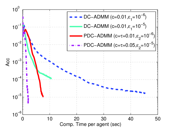
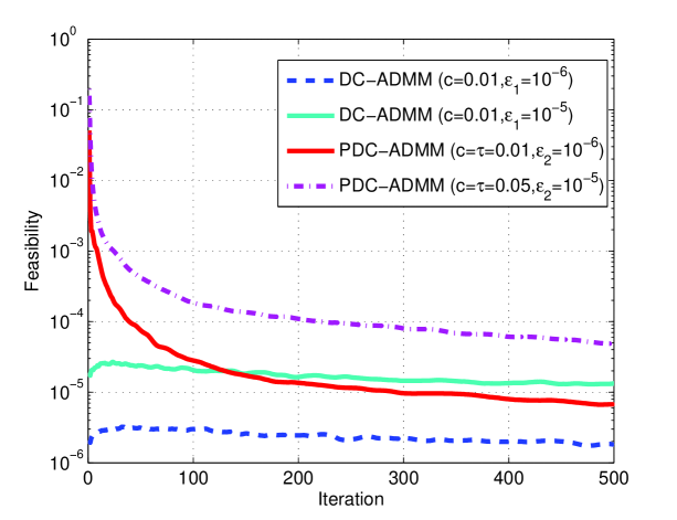
Figure 1: Convergence curves of DC-ADMM and PDC-ADMM.
Example 1: We first consider the performance comparison between DC-ADMM and PDC-ADMM. Table I(a) shows the comparison results for , , , and . For PDC-ADMM, we simply set and .
The penalty parameters of the two algorithms are respectively chosen so that the two algorithms can exhibit best convergence behaviors444We did not perform exhaustive search. Instead, we simply pick the value of from the set for which the algorithm can yield best convergence behavior for a randomly generated problem instance and graph. Once the value of is determined, it is fixed and tested for another 9 randomly generated problem instances and graphs.. One can see from Table I(a) that DC-ADMM (, , )555The parameter is also chosen in a similar fashion as the parameter . can achieve the stopping condition AccFeas with an average iteration number but spends an average per-agent computation time of 19.63 seconds. One should note that a naive way to reducing the computation time of DC-ADMM is to reduce the solution accuracy of subproblem (3), i.e., increasing . As seen, DC-ADMM with has a reduced per-agent computation time 9.87 seconds; however, the required iteration number drastically increases to 980.1. By contrast, one can see from Table I(a) that the proposed PDC-ADMM (, ) can achieve the stopping condition with an average iteration number and a much less (per-agent) computation time seconds. If one reduces the solution accuracy of BSUM for solving subproblem (3) to , then the computation time of PDC-ADMM can further reduce to 1.58 seconds, though the required iteration number is increased to 298.8. Figure 1 displays the convergence curves of DC-ADMM and PDC-ADMM for one of the 10 randomly generated problem instances. One can see from Fig. 1(a) that PDC-ADMM (, ) has a comparable convergence behavior as DC-ADMM (, , ) when with respect to the iteration number and in terms of the solution accuracy Acc. Moreover, as seen from Fig. 1(b), when with respect to the computation time, PDC-ADMM (, ) is much faster than DC-ADMM (, , ). However, it is seen from Fig. 1(c) that DC-ADMM usually has a small value of feasibility Feas which is understandable as the constraint is explicitly handled in subproblem (3); whereas the constraint feasibility associated with PDC-ADMM gradually decreases with the iteration number.
This explains why in Table I(a), to achieve AccFeas , PDC-ADMM always has smaller values of Acc than DC-ADMM but has larger values of Feas.
In summary, by comparing to the naive strategy of reducing the solution accuracy of (3) in DC-ADMM, we observe that the proposed PDC-ADMM can achieve a much better tradeoff between the iteration number and computation time. Since the iteration number is also the number of message exchanges between connecting agents, the results equivalently show that the proposed PDC-ADMM achieves a better tradeoff between communication overhead and computational complexity.
In Table I(b), we present another set of simulation results for , , , and . One can still observe that the proposed PDC-ADMM has a better tradeoff between the iteration number and computation time compared to DC-ADMM. In particular, one can see that, for DC-ADMM with reduced from to , reduction of the computation time is limited but the iteration number increased to a large number of 1173.
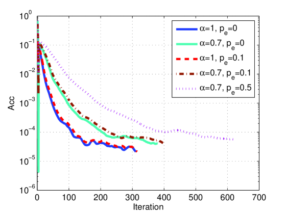
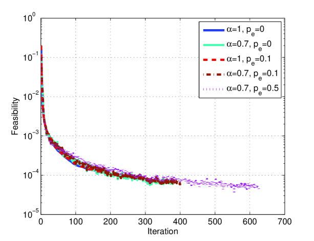
Example 2: In this example, we examine the convergence behavior of randomized PDC-ADMM (Algorithm 3). It is set that , i.e., all agents have the same active probability. Note that, for and , randomized PDC-ADMM performs identically as the PDC-ADMM in Algorithm 1. Figure 2 presents the convergence curves of randomized PDC-ADMM for different values of and and for the stopping condition being AccFeas .
The simulation setting and problem instance are the same as that used for PDC-ADMM (, ) in Fig. 1.
One can see from Fig. 2(a) that no matter when decreases to and/or increases to , randomized PDC-ADMM always exhibits consistent convergence behavior, though the convergence speed decreases accordingly.
We also observe from Fig. 2(a) that Acc may oscillate in the first few iterations when and . Interestingly, from Fig. 2(b), one can observe that the values of and do not affect the convergence behavior of constraint feasibility much.
Figure 2: Convergence curves of randomized PDC-ADMM.
VI Conclusions
In this paper, we have
proposed two ADMM based distributed optimization methods, namely the PDC-ADMM method (Algorithm 1) and the randomized PDC-ADMM method (Algorithm 3) for the polyhedra constrained problem (P). In contrast to the existing DC-ADMM where each agent requires to solve a polyhedra constrained subproblem at each iteration, agents in the proposed PDC-ADMM and randomized PDC-ADMM methods deal with a subproblem with simple constraints only, thereby more efficiently implementable than DC-ADMM. For both proposed PDC-ADMM and randomized PDC-ADMM, we have shown that they have a worst-case convergence rate. The presented simulation results based on the constrained LASSO problem in (2) have shown that the proposed PDC-ADMM method exhibits a much lower computation time than DC-ADMM, although the required iteration number is larger.
It has been observed that the tradeoff between communication overhead and computational complexity of PDC-ADMM is
much better, especially when comparing to the naive strategy of reducing the subproblem solution accuracy of DC-ADMM. It has been also shown that the proposed randomized PDC-ADMM method can converge consistently in the presence of randomly ON/OFF agents and severely unreliable links.
VII Acknowledgement
The author would like to thank Prof. Min Tao at the Nanjing University for her valuable discussions.
By (7) and (20), subproblem (17) can be explicitly written as a min-max problem as follows
(A.5)
where
(A.6)
Notice that is (strongly) convex with respect to given any and is concave with respect to given any .
Therefore, the minimax theorem [27, Proposition 2.6.2] can be applied
so that saddle point exists for (B) and it is equivalent to its max-min counterpart
(A.7)
Let and be a pair of saddle point of (B) and (A.7).
Then, given , is the unique inner minimizer of (A.7), which, from (B), can be readily obtained as the closed-form solutions in (22) and (22b), respectively. By substituting (22) and (22b)
into (A.7), can be obtain by subproblem (III).
We remark here that if one removes the dummy constraint from (8) and the augmented term from (III), then the corresponding subproblem (17) reduces to
(A.8)
Note that (B) is no longer strongly convex with respect to as the term is absent. After applying the minmax theorem to (B):
one can see that, to have a bounded optimal value for the inner minimization problem, it must hold , and thus appears redundant. Moreover, one can show that the inner optimal is
(A.9)
where
(A.10)
The variable also appears redundant and can be removed from (B). The resultant steps of (B), (B) and (21) are the DC-ADMM method in [19] (see Algorithm 2).
Notice that we have recovered from according to (18), (19), and (21).
Besides, the update orders of and are reversed here for ease of the analysis.
According to [14, Lemma 4.1], the optimality condition of (C) with respect to is given by: ,
(A.16)
where the equality is obtained by using (A.14) and (A.15). Analogously, the optimality condition of (C) with respect to is given by, ,
(A.17)
where the equality is owing to (A.15).
By summing (C) and (C), one obtains
(A.18)
By letting and for all in (C), where denotes the optimal solution to problem (5), we have the following chain from (C)
(A.20)
where the first equality is due to the fact ; the second equality is obtained by adding and subtracting both terms and for arbitrary and ; the last equality is due to (A.15).
On the other hand, note that (A.14) can be expressed as
(A.21)
where the last equality is obtained by applying (A.11) and (A.12).
Furthermore, let be an optimal solution to problem (8), and denote be an optimal dual solution of (8). Then, according to the Karush-Kuhn-Tucker (KKT) condition [31], we have
(A.22)
where denotes a subgradient of with respect to at point .
Since under Assumption 1, and form a pair of primal-dual solution
to problem (5) under Assumption 2, is optimal to (7) given , and thus [37], which and (A.22) give rise to
(A.23)
By combing (C) and (A.23) followed by multiplying on both sides of the resultant equation, one obtains
(A.24)
By further substituting (C) into (C) and summing for , one obtains that
(A.25)
for arbitrary and , where .
By following the same idea as in [19, Eqn. (A.16)], one can show that
(A.26)
where , and (see [19, Remark 1]). Moreover, according to [19, Eqn. (A.15)], it can be shown that
(A.27)
where () is a vector that stacks () for all and . As a result, (C) can be expressed as
The proof is based on the “full iterates” assuming that all agents and all edges are active at iteration . Specifically, the full iterates for iteration are
(A.36)
(A.37)
(A.38)
(A.39)
(A.40)
(A.41)
It is worthwhile to note that
(A.42)
(A.43)
Let us consider the optimality condition of (D). Following similar steps as in (C) to (C), one can have that
where the third equality is due to (A.40) and (A.41),
and the last equality is obtained by invoking (A.23).
By multiplying with the last two terms in (D), we obtain
(A.46)
By substituting (D) into (D) and summing the equations for , one obtains
(A.47)
Also note that
(A.48)
where the first equality is obtained by the fact that, for any ,
(A.49)
owing to the symmetric property of ; the second equality is due to the fact of and for all and ; the third equality is from (A.39); the fourth equality is by defining () as a vector that stacks () for all , ; and the last inequality is obtained by applying (C).
Then, similar to the derivations from (C) to (C),
one can deduce from (D) and (D) that
(A.50)
where
(A.51)
To connect the full iterates with the instantaneous iterates, let us define a weighed Lagrangian as
(A.52)
Moreover, let be the set of historical events up to iteration . By (A.42) and (3), the conditional expectation of can be shown as
(A.53)
where the last inequality is due to (D). Furthermore, define
(A.54)
(A.55)
(A.56)
Then, by (A.42), (A.43) and (3), one can show that
(A.57)
(A.58)
(A.59)
By substituting (D), (A.58) and (A.59) into (D) followed by taking the expectation with respect to , one obtains
Upon summing the above equation from , and taking the average, we can obtain the following bound
(A.60)
Similar to (C) and (C), by letting and
, one can bound the feasibility of from (D) as
(A.61)
where
(A.62)
Also similar to (C) and (A.35), by letting and , one can bound the expected objective value as
[1]
B. Yang and M. Johansson, “Distributed optimization and games: A tutorial
overview,” Chapter 4 of Networked Control Systems, A. Bemporad, M.
Heemels and M. Johansson (eds.), LNCIS 406, Springer-Verlag, 2010.
[2]
V. Lesser, C. Ortiz, and M. Tambe, Distributed Sensor Networks: A
Multiagent Perspective. Kluwer
Academic Publishers, 2003.
[3]
I. Foster, Y. Zhao, I. Raicu, and S. Lu, “Cloud computing and grid computing
360-degree compared,” in Proc. Grid Computing Environments Workshop,
Austin, TX, USA, Nov. 12-16, 2008, pp. 1–10.
[4]
R. Bekkerman, M. Bilenko, and J. Langford, Scaling up Machine Learning-
Parallel and Distributed Approaches. Cambridge University Press, 2012.
[5]
S. Chen, D. Donoho, and M. Saunders, “Atomic decomposition by basis pursuit,”
SIAM J. Sci. Comput., vol. 20, no. 1, pp. 33–61, 1998.
[6]
T. Hastie, R. Tibshirani, and J. Friedman, The Elements of Statistical
Learning: Data Mining, Inference, and Prediction. New York, NY, USA: Springer-Verlag, 2001.
[7]
M. Alizadeh, X. Li, Z. Wang, A. Scaglione, and R. Melton, “Demand side
management in the smart grid: Information processing for the power
switch,” IEEE Signal Process. Mag., vol. 59, no. 5, pp. 55–67, Sept.
2012.
[8]
D. P. Bertsekas, Network Optimization : Contribuous and Discrete
Models. Athena Scientific, 1998.
[9]
C. Shen, T.-H. Chang, K.-Y. Wang, Z. Qiu, and C.-Y. Chi, “Distributed robust
multicell coordianted beamforming with imperfect CSI: An ADMM approach,”
IEEE Trans. Signal Process., vol. 60, no. 6, pp. 2988–3003, 2012.
[10]
A. Nedic and A. Ozdaglar, “Distributed subgradient methods for multi-agent
optimization,” IEEE Trans. Auto. Control, vol. 54, no. 1, pp. 48–61,
Jan. 2009.
[11]
M. Zhu and S. Martínez, “On distributed convex optimization under
inequality and equality constraints,” IEEE Trans. Auto. Control,
vol. 57, no. 1, pp. 151–164, Jan. 2012.
[12]
J. Chen and A. H. Sayed, “Diffusion adaption strategies for distributed
optimization and learning networks,” IEEE. Trans. Signal Process.,
vol. 60, no. 8, pp. 4289–4305, Aug. 2012.
[13]
T.-H. Chang, A. Nedić, and A. Scaglione, “Distributed constrained
optimization by consensus-based primal-dual perturbation method,”
IEEE. Trans. Auto. Control., vol. 59, no. 6, pp. 1524–1538, June
2014.
[14]
D. P. Bertsekas and J. N. Tsitsiklis, Parallel and distributed
computation: Numerical methods. Upper Saddle River, NJ, USA: Prentice-Hall, Inc., 1989.
[15]
S. Boyd, N. Parikh, E. Chu, B. Peleato, and J. Eckstein, “Distributed
optimization and statistical learning via the alternating direction method of
multipliers,” Foundations and Trends in Machine Learning, vol. 3,
no. 1, pp. 1–122, 2011.
[16]
G. Mateos, J. A. Bazerque, and G. B. Giannakis, “Distributed sparse linear
regression,” IEEE Trans. Signal Process., vol. 58, no. 10, pp.
5262–5276, Dec. 2010.
[17]
J. F. C. Mota, J. M. F. Xavier, P. M. Q. Aguiar, and M. Puschel, “Distributed
basis pursuit,” IEEE. Trans. Signal Process., vol. 60, no. 4, pp.
1942–1956, April 2012.
[18]
——, “D-ADMM: A communication-efficient distributed algorithm for
separable optimization,” IEEE. Trans. Signal Process., vol. 60,
no. 10, pp. 2718–2723, May 2013.
[19]
T.-H. Chang, M. Hong, and X. Wang, “Multi-agent distributed optimization via
inexact consensus ADMM,” submitted to IEEE Trans. Signal Process.;
available on arxiv.org.
[20]
W. Shi, Q. Ling, K. Yuan, G. Wu, and W. Yin, “On the linear convergence of the
ADMM in decentralized consensus optimization,” IEEE Trans. Signal
Process., vol. 62, no. 7, pp. 1750–1761, April 2014.
[21]
E. Wei and A. Ozdaglar, “On the convergence of asynchronous
distributed alternating direction method of multipliers,” available on
arxiv.org.
[22]
D. P. Bertsekas, Nonlinear Programming: 2nd Ed. Cambridge, Massachusetts: Athena Scientific, 2003.
[23]
T.-H. Chang, M. Alizadeh, and A. Scaglione, “Coordinated home energy
management for real-time power balancing,” in Proc. IEEE PES General
Meeting, San Diego, CA, July 22-26, 2012, pp. 1–8.
[24]
Y. Zhang and G. B. Giannakis, “Efficient decentralized economic dispatch for
microgrids with wind power integration,” available on arxiv.org.
[25]
S. S. Ram, A. Nedić, and V. V. Veeravalli, “A new class of distributed
optimization algorithm: Application of regression of distributed data,”
Optimization Methods and Software, vol. 27, no. 1, pp. 71–88, 2012.
[26]
G. M. James, C. Paulson, and P. Rusmevichientong, “The constrained Lasso,”
working paper, available on http://www-bcf.usc.edu/~rusmevic/.
[27]
D. P. Bertsekas, A. Nedić, and A. E. Ozdaglar, Convex analysis and
optimization. Cambridge,
Massachusetts: Athena Scientific, 2003.
[28]
L. Grippo and M. Sciandrone, “On the convergence of the block nonlinear
gauss-seidel method under convex constraints,” Operation research
letter, vol. 26, pp. 127–136, 2000.
[29]
M. Razaviyayn, M. Hong, and Z.-Q. Luo, “A unified convergence analysis of
block successive minimization methods for nonsmooth optimization,”
SIAM J. OPtim., vol. 23, no. 2, pp. 1126–1153, 2013.
[30]
A. Beck and M. Teboulle, “A fast iterative shrinkage-thresholding algorithm
for linear inverse problems,” SIAM J. Imaging Sci., vol. 2, no. 1,
pp. 183–202, 2009.
[31]
S. Boyd and L. Vandenberghe, Convex Optimization. Cambridge, UK: Cambridge University Press, 2004.
[32]
M. Hong, T.-H. Chang, X. Wang, M. Razaviyayn, S. Ma, and Z.-Q. Luo, “A block
successive upper bound minimization method of multipliers for linearly
constrained convex optimization,” submittd to SIAM J. Opt. available
on arxiv.org.
[33]
Y. Nesterov, “Smooth minimization of nonsmooth functions,” Math.
Program., vol. 103, no. 1, pp. 127–152, 2005.
[34]
P. L. Combettes and J.-C. Pesquet, “Proximal splitting methods in signal
processing,” available on arxiv.org.
[35]
M. Grant and S. Boyd, “CVX: Matlab software for disciplined convex
programming, version 1.21,” http://cvxr.com/cvx, Apr. 2011.
[36]
M. E. Yildiz and A. Scaglione, “Coding with side information for
rate-constrained consensus,” IEEE Trans. Signal Process., vol. 56,
no. 8, pp. 3753–3764, 2008.
[37]
S. Boyd and A. Mutapcic, “Subgradient methods,” avaliable at
www.stanford.edu/class/ee392o/subgrad_method.pdf.