Fixed-point quantum search with an optimal number of queries

Abstract

Grover’s quantum search and its generalization, quantum amplitude amplification, provide quadratic advantage over classical algorithms for a diverse set of tasks, but are tricky to use without knowing beforehand what fraction $\lambda$ of the initial state is comprised of the target states. In contrast, fixed-point search algorithms need only a reliable lower bound on this fraction, but, as a consequence, lose the very quadratic advantage that makes Grover’s algorithm so appealing. Here we provide the first version of amplitude amplification that achieves fixed-point behavior without sacrificing the quantum speedup. Our result incorporates an adjustable bound on the failure probability, and, for a given number of oracle queries, guarantees that this bound is satisfied over the broadest possible range of $\lambda$.

Grover’s quantum search algorithm Grover (1996) provides a quadratic speedup over classical algorithms for solving a broad class of problems. Included are the many important, yet computationally prohibitive NP problems Bennett et al. (1997), for which finding a solution reduces to searching for one. Because the problem Grover’s algorithm solves is so simple to understand – given an oracle function that recognizes marked items, locate one of $M$ such marked items amongst $N$ unsorted items – its classical time complexity $\mathcal{O}(N/M)$ is obvious, making the quantum speedup that much more conclusive.

Conceptually also, Grover’s algorithm is compelling – the iterative application of the oracle and initial state preparation rotates from a superposition of mostly unmarked states to a superposition of mostly marked states in just $\mathcal{O}(\sqrt{N/M})$ steps Aharonov (1998). This interpretation of Grover’s algorithm as a rotation is very natural because the Grover iterate is a unitary operator. However, this same unitarity is also a weakness. Without knowing exactly how many marked items there are, there is no knowing when to stop the iteration! This leads to the soufflé problem Brassard (1997), in which iterating too little “undercooks” the state, leaving mostly unmarked states, and iterating too much “overcooks” the state, passing by the marked states and leaving us again with mostly unmarked states.

The most direct solution of the soufflé problem is to estimate $M$ by either using full-blown quantum counting Boyer et al. (1998); Brassard et al. (1998) or a trial-and-error scheme where iterates are applied an exponentially increasing number of times Boyer et al. (1998); Brassard et al. (2000). Although scaling quantumly, these strategies are unappealing for search as they work best not by monotonically amplifying marked states, but rather by getting “close enough” before resorting to classical random sampling.

An alternative approach, in line with what we advocate here, is to construct, either recursively or dissipatively, operators that avoid overcooking by always amplifying marked states. Such algorithms are known as fixed-point searches. For example, running Grover’s $\pi/3$-algorithm Grover (2005) or the comparable ancilla-algorithm Grover et al. (2006) longer can only ever improve its success probability. Yet, a steep price is paid for this monotonicity – in both cases, the quadratic speedup of the original quantum search is lost.

This disappointing fact means that current fixed-point algorithms take time $\mathcal{O}(N/M)$ for small $M/N$, and their usefulness is relegated to large $M/N$, where they conveniently avoid overcooking, but where classical algorithms are also already successful. Several results Li and Li (2007); Toyama et al. (2009) improve the performance of fixed-point algorithms on wide ranges of $M/N$, but these algorithms are numerical and as such their time scaling cannot be assessed. Indeed, the $\pi/3$-algorithm was shown to be optimal in time Chakraborty et al. (2005), ostensibly proving it impossible to find a search algorithm that both avoids the soufflé problem and provides a quantum advantage.

Nevertheless, here we present a fixed-point search algorithm, which, amazingly, achieves both goals – our search procedure cannot be overcooked and also achieves optimal time scaling, a quadratic advantage over classical unordered search. We sidestep the conditions of the impossibility proof by requiring not that the error monotonically improve as in the $\pi/3$-algorithm, but that the error become bounded by a tunable parameter $\delta$ over an ever widening range of $M/N$ as our algorithm is run longer. The polynomial method Beals et al. (2001) is typically used to prove lower bounds on quantum query complexities; however, we instead use the fact that the success probability is a polynomial to adjust the phases of Grover’s reflection operators Long et al. (1999); Høyer (2000) and effect an optimal output polynomial with bounded error $\delta$. In fact, our algorithm becomes the $\pi/3$-algorithm and Grover’s original search algorithm in the special cases of $\delta=0$ and $\delta=1$, respectively.

Our results apply just as cleanly, and more generally, to amplitude amplification Brassard et al. (2000), so we proceed in that framework. We are given a unitary operator $A$ that prepares the initial state $|s\rangle=A|0\rangle^{\otimes n}$. From $|s\rangle$, we would like to extract the target state $|T\rangle$ with success probability $P_{L}\geq 1-\delta^{2}$, where the overlap $\langle T|s\rangle=\sqrt{\lambda}e^{i\xi}$ is not zero and $\delta\in[0,1]$ is given. To do so, we are provided with the oracle $U$ which flips an ancilla qubit when fed the target state. That is, $U|T\rangle|b\rangle=|T\rangle|b\oplus 1\rangle$ and $U|\overline{T}\rangle|b\rangle=|\overline{T}\rangle|b\rangle$ for $\langle\overline{T}|T\rangle=0$. Below, we show how to solve this problem and extract $|T\rangle$ by performing on $|s\rangle$ a quantum circuit $\mathcal{S}_{L}$ consisting of $A,A^{\dagger},U$, and efficiently implementable $n$-qubit gates, such that

$$P_{L}=|\langle T|\mathcal{S}_{L}|s\rangle|^{2}=1-\delta^{2}\text{ }T_{L}\left(T_{1/L}(1/\delta)\sqrt{1-\lambda}\right)^{2}.$$ (1)

Here $T_{L}(x)=\cos(L\cos^{-1}(x))$ is the $L^{\text{th}}$ Chebyshev polynomial of the first kind Rivlin (1990) and $L-1$ is the query complexity: the number of times $U$ is applied in the circuit $\mathcal{S}_{L}$. Furthermore, we will construct $\mathcal{S}_{L}$ for any odd integer $L\geq 1$ and any $\delta$. Some examples of $P_{L}$ and a comparison to the $\pi/3$-algorithm are shown in Fig. 1.

Assuming for now the existence of $\mathcal{S}_{L}$ – its construction will be given later – we can already see that the success probability $P_{L}$ possesses both the fixed point property and optimal query complexity. First, note that as long as $|T_{1/L}(1/\delta)|\sqrt{1-\lambda}\leq 1$, the fact that $|T_{L}(x)|\leq 1$ for $|x|\leq 1$ implies $P_{L}\geq 1-\delta^{2}$. Therefore, for all $\lambda\geq w=1-T_{1/L}(1/\delta)^{-2}$, the probability $P_{L}$ meets our error tolerance. For large $L$ and small $\delta$, this width $w$ can be approximated as

$$w\approx\left(\frac{\log(2/\delta)}{L}\right)^{2}.$$ (2)

This equation demonstrates the fixed-point property – as $L$ increases, $w$ decreases, and we achieve success probability $P_{L}\geq 1-\delta^{2}$ over an ever increasing range of $\lambda$. Equivalently, this means we cannot overcook the state, because if a sequence $\mathcal{S}_{L}$ achieves bounded error at $\lambda$, then so does $\mathcal{S}_{L^{\prime}}$ for any $L^{\prime}>L$. Second, note that to ensure the probability is bounded we must choose $L$ such that $w\leq\lambda$. That is, for $\delta>0$,

$$L\geq\frac{\log(2/\delta)}{\sqrt{\lambda}}.$$ (3)

Thus, query complexity goes as $L=\mathcal{O}\left(\log(2/\delta)\frac{1}{\sqrt{\lambda}}\right)$ for our algorithm, achieving, for amplitude amplification, the best possible scaling in $\lambda$ Brassard et al. (2000). See also Fig. 1 (inset).

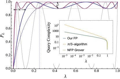
Figure 1: A comparison of search algorithms, plotting the overlap $P_{L}$ of the target state with the output state versus the overlap $\lambda$ of the target state with the initial state. We weigh our fixed-point (FP) algorithm (thick solid) against the $\pi/3$-algorithm (dashed) for the task of achieving output success probability $P_{L}$ greater than $1-\delta^{2}=0.9$ for all $\lambda>\lambda_{0}$. The query complexity of the algorithms vary based on $\lambda_{0}$ (dotted vertical lines). For $\lambda_{0}=0.25$ (blue), our algorithm makes $4$ queries while the $\pi/3$-algorithm makes $8$. For $\lambda_{0}=0.03$ (red), our algorithm makes $12$ queries while the $\pi/3$-algorithm makes $80$. For comparison, also shown is Grover’s non-fixed-point (NFP) search with 8 queries (thin black). The width and error for our 4-query algorithm are labeled $w$ and $\delta$, respectively. (Inset) We plot the query complexity against $\lambda$ for our algorithm with $\delta^{2}=0.1$ (solid), the $\pi/3$-algorithm (dashed), and non-fixed-point Grover’s (dotted). While our FP algorthm and Grover’s NFP algorithm scale as $L\sim 1/\sqrt{\lambda}$, the $\pi/3$-algorithm scales as $L\sim 1/\lambda$.

Having seen two defining attributes, the fixed-point property and optimality, of the success probability from Eq. (1), let us now create it using the operators provided: the state preparation $A$ and oracle $U$. This problem simplifies when interpreted in the two-dimensional subspace $\mathcal{T}$ spanned by $|s\rangle$ and $|T\rangle$ rather than in the full $2^{n}$-dimensional Hilbert space of all $n$ qubits. First, define $|t\rangle=e^{-i\xi}|T\rangle$ and $|\overline{t}\rangle=\big{(}|s\rangle-\langle t|s\rangle|t\rangle\big{)}/\sqrt{1-\lambda}$, so that

$$|s\rangle=\sqrt{1-\lambda}|\overline{t}\rangle+\sqrt{\lambda}|t\rangle=\left(\begin{array}[]{c}\sqrt{1-\lambda}\\ \sqrt{\lambda}\end{array}\right).$$ (4)

The matrix notation comes from the definitions $|t\rangle=\left(\begin{smallmatrix}0\\ 1\end{smallmatrix}\right)$ and $|\overline{t}\rangle=\left(\begin{smallmatrix}1\\ 0\end{smallmatrix}\right)$. The location of $|s\rangle$ on the Bloch sphere is in the XZ-plane at an angle $\phi$ from the north pole, where $\phi\in[0,\pi]$ is defined by $\sin(\phi/2)=\sqrt{\lambda}$. Our goal of achieving the $P_{L}$ of Eq. (1) is equivalently expressed as constructing, up to a global phase, the Chebyshev state

$$|C_{L}\rangle=\sqrt{1-P_{L}}|\overline{t}\rangle+\sqrt{P_{L}}e^{i\chi}|t\rangle=\left(\begin{array}[]{c}\sqrt{1-P_{L}}\\ \sqrt{P_{L}}e^{i\chi}\end{array}\right)$$ (5)

for some relative phase $\chi$. For large enough $\lambda$, the Chebyshev state lies near the south pole of the Bloch sphere.

Similarly, Grover’s reflection operators can be interpreted as $\text{SU}(2)$ unitaries acting on $\mathcal{T}$. As in previous work Long et al. (1999); Høyer (2000), we add arbitrary phases to the reflections to define generalized reflections. In Fig. 2 we show explicitly how to implement these generalized reflections using $A$, $U$, and efficiently implementable $n$-qubit operations. Their $\text{SU}(2)$ representations are

$$S_{s}(\alpha) =I-(1-e^{-i\alpha})|s\rangle\langle s|$$ (6)

$$=\left(\begin{array}[]{cc}1-(1-e^{-i\alpha})\overline{\lambda}&-(1-e^{-i\alpha})\sqrt{\lambda\overline{\lambda}}\\ -(1-e^{-i\alpha})\sqrt{\lambda\overline{\lambda}}&1-(1-e^{-i\alpha})\lambda\end{array}\right),$$ (9)

$$S_{t}(\beta) =I-(1-e^{i\beta})|t\rangle\langle t|=\left(\begin{array}[]{cc}1&0\\ 0&e^{i\beta}\end{array}\right),$$ (12)

where $\overline{\lambda}=1-\lambda$. The product of the reflection operators is often called the Grover iterate $G(\alpha,\beta)=-S_{s}(\alpha)S_{t}(\beta)$. The original Grover iterate Grover (1996) used $\alpha=\pm\pi$ and $\beta=\pm\pi$.

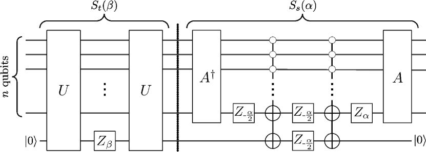
Figure 2: We provide a circuit for performing the generalized Grover iterate $G(\alpha,\beta)$ up to a global phase. Here, $Z_{\theta}:=R_{0}(\theta)$ represents a rotation about the z-axis by angle $\theta$. The first part of the circuit, before the dotted line, performs $e^{-i\beta/2}S_{t}(\beta)$ and the second part performs $S_{s}(\alpha)$. One ancilla bit initialized as $|0\rangle$ is required for both parts, but can be reused. The multiply-controlled NOT gates in the $S_{s}(\alpha)$ circuit do not pose a substantial overhead – they can be implemented with $\mathcal{O}(n^{2})$ single qubit and CNOT gates Saeedi and Pedram (2013) or $\mathcal{O}(n)$ such gates and $\mathcal{O}(n)$ ancillas Nielsen and Chuang (2004).

The generalized reflection operators are also expressible as rotations on the Bloch sphere. Defining $R_{\varphi}(\theta)=\exp\left(-i\frac{1}{2}\theta(\cos(\varphi)Z+\sin(\varphi)X)\right)$ for Pauli operators $X$ and $Z$, we find

$$S_{s}(\alpha) =e^{-i\alpha/2}R_{\phi}(\alpha)$$ (13)

$$S_{t}(\beta) =e^{i\beta/2}R_{0}(\beta).$$ (14)

When $\alpha=\pm\pi$ and $\beta=\pm\pi$, these rotations map the XZ-plane to the XZ-plane, reproducing the $\text{O}(1)$ rotation picture of Grover’s original non-fixed-point algorithm Aharonov (1998).

Yet, why limit ourselves to $O(1)$ when, by using general phases $\alpha$ and $\beta$, we can access the whole of $\text{SU}(2)$? To that end, we consider a sequence of $l$ generalized Grover iterates. Since each generalized Grover iterate contains two queries to $U$, such a sequence would have query complexity $L-1=2l$. We thus set out to find, for any $\lambda>0$, phases $\alpha_{j}$ and $\beta_{j}$ such that the sequence

$$\mathcal{S}_{L}=G(\alpha_{l},\beta_{l})\dots G(\alpha_{1},\beta_{1})=\prod_{j=1}^{l}G(\alpha_{j},\beta_{j})$$ (15)

attains success probability $P_{L}$ by preparing, up to a global phase, the Chebyshev state: $|\langle C_{L}|\mathcal{S}_{L}|s\rangle|=1$.

Indeed, such phases exist for all $l$ and all $\delta\in[0,1]$, and, moreover, they may be given in very simple analytical forms. For all $j=1,2,\dots,l$, we have

$$\alpha_{j}=-\beta_{l-j+1}=2\cot^{-1}\left(\tan(2\pi j/L)\sqrt{1-\gamma^{2}}\right),$$ (16)

where $L=2l+1$ as before and $\gamma^{-1}=T_{1/L}\left(1/\delta\right)$. Notice Grover’s non-fixed-point search is subsumed by this solution – if $\delta=1$, then $\alpha_{j}=\pm\pi$ and $\beta_{j}=\pm\pi$ for all $j$, values that we saw above give Grover’s original non-fixed-point algorithm Grover (1996). Thus, when $\delta=1$, our algorithm is exactly Grover’s search.

The proof that Eq. (16) implies Eq. (1) begins by rearranging $\mathcal{S}_{L}$. Let $A_{\zeta}=\exp(-i\frac{1}{2}\phi(\cos(\zeta)X+\sin(\zeta)Y))$. With this definition, the state preparation operator is $A=A_{\pi/2}$. Also note the identities $R_{\phi}(\alpha)=A_{\pi/2}R_{0}(\alpha)A_{-\pi/2}$ and $A_{\alpha+\beta}=R_{0}(\beta)A_{\alpha}R_{0}(-\beta)$. Then, using Eqs. (13-14), we find, up to a global phase, that

$$\mathcal{S}_{L}|s\rangle\sim R_{0}(\zeta_{1})\left(A_{\zeta_{L}}\dots A_{\zeta_{2}}A_{\zeta_{1}}\right)R_{0}(-\zeta_{1})|0\rangle.$$ (17)

Here the phases $\zeta_{k}=\zeta_{L-k+1}$ are palindromic, a consequence of the phase matching $\alpha_{j}=-\beta_{l-j+1}$. With $\alpha_{j}$ defined by Eq. (16), all $\zeta_{k}$ can be found recursively using $\zeta_{l+1}=(-1)^{l}\pi/2$ and

$$\zeta_{k+1}-\zeta_{k}=(-1)^{k}\pi-2\cot^{-1}\left(\tan(k\pi/L)\sqrt{1-\gamma^{2}}\right)$$ (18)

for all $k=1,\dots,L-1$.

From Eq. (17), we set up a recurrence relation to study the amplitude in states $|t\rangle$ and $|\overline{t}\rangle$ after each application of $A_{\zeta}$. That is, we let $(a_{0},b_{0})=(1,0)$ and for $h=1,\dots,L$ define $a_{h}$ and $b_{h}$ by the matrix equation

$$\left(\begin{array}[]{c}a_{h}\\ b_{h}\sin(\phi/2)\end{array}\right)=A_{\zeta_{h}}\left(\begin{array}[]{c}a_{h-1}\\ b_{h-1}\sin(\phi/2)\end{array}\right).$$ (19)

Letting $x=\cos(\phi/2)$, we can decouple this recurrence by defining $b^{\prime}_{h}=-xa_{h}-i\sqrt{1-x^{2}}e^{-i\zeta_{h}}b_{h}$. Rearranging Eq. (19), we find $b^{\prime}_{h}=-a_{h-1}$ and

$$a_{h}=x(1+e^{-i(\zeta_{h}-\zeta_{h-1})})a_{h-1}-e^{-i(\zeta_{h}-\zeta_{h-1})}a_{h-2},$$ (20)

for $h=2,\dots,L$ with initial values $a_{0}=1$ and $a_{1}=x$. This recurrence is strikingly similar to that defining the Chebyshev polynomials: $T_{n}(x)=2xT_{n-1}(x)-T_{n-2}(x)$. Indeed, using Eq. (18), the Chebyshev recurrence is exactly recovered when $\gamma=\delta=1$. For other values of $\gamma$, the complex, degree-$h$ polynomials $a_{h}^{(\gamma)}(x)$ generalize the Chebyshev polynomials. In fact, it can be shown using combinatorial arguments analogous to those in Benjamin and Walton (2009) that $a^{(\gamma)}_{L}(x)=\frac{T_{L}(x/\gamma)}{T_{L}(1/\gamma)}$. Since $T_{L}(1/\gamma)=1/\delta$ and $P_{L}=1-|a^{(\gamma)}_{L}(x)|^{2}$, this completes the proof of Eq. (1).

While the solutions in Eq. (16) are extremely simple to express, there are other solutions. Indeed, solutions of small length $l$ and large width $w$ can be combined to create solutions of larger length and smaller width through a process we call nesting. The general idea of nesting is that, within a sequence $\mathcal{S}_{L_{2}}$, the state preparation $A$ can be replaced by another sequence $\mathcal{S}_{L_{1}}A$ to recursively narrow the region of high failure probability. An intuition for this recursion can be noted in the similarity of Eq. (4) and Eq. (5). Nesting is similar to concatenation in composite pulse sequence literature Jones (2013) and has already been employed in special cases of fixed-point search Grover (2005).

Although nesting would work to widen any fixed-point sequence (those found in Li and Li (2007); Toyama et al. (2009), for instance), with our sequences using phases from Eq. (16), nesting neatly preserves the form of the success probability $P_{L}$. For notational convenience let us denote by $\mathcal{S}_{L}(B)$ a sequence of generalized Grover iterates as in Eq. (15) that uses $BA$ in place of the state preparation operator $A$. For instance, with $I$ the identity operator, we know

$$\mathcal{S}_{L_{1}}\left(I\right)|s\rangle=\sqrt{1-P_{L_{1}}(\lambda)}|\overline{t}\rangle+\sqrt{P_{L_{1}}(\lambda)}e^{i\chi_{1}}|t\rangle,$$ (21)

where we have made explicit the dependence of $P_{L}$ from Eq. (1) on $\lambda$. By the same logic,

$$\mathcal{S}_{L_{2}}\left(\mathcal{S}_{L_{1}}(I)\right)\mathcal{S}_{L_{1}}(I)|s\rangle =\sqrt{1-P_{L_{2}}\left(P_{L_{1}}(\lambda)\right)}|\overline{t}\rangle$$ (22)

$$+\sqrt{P_{L_{2}}\left(P_{L_{1}}(\lambda)\right)}e^{i(\chi_{1}+\chi_{2})}|t\rangle.$$

Consider $P_{L_{2}}\left(P_{L_{1}}(\lambda)\right)$ and say that we choose the error bound for sequence 1 to be $\delta_{1}=\left(T_{1/L_{2}}\left[1/\delta\right]\right)^{-1}$ and that for sequence 2 to be $\delta_{2}=\delta$. Using the semi-group property of the Chebyshev polynomials, $T_{p}\left(T_{q}\left(x\right)\right)=T_{pq}(x)$, simple algebra yields

$$P_{L_{2}}\left(P_{L_{1}}(\lambda,\delta_{1}),\delta_{2}\right)=P_{L_{1}L_{2}}(\lambda,\delta),$$ (23)

where we have further explicated the dependence of $P_{L}$ from Eq. (1) on its error bound $\delta$.

Therefore, as a result of nesting we can combine sequences of complexities $L_{1}$ and $L_{2}$ to obtain a sequence of complexity $L_{1}L_{2}$. In terms of Grover iterations, sequences with $l_{1}$ and $l_{2}$ iterations can be combined into one with $l=l_{1}+2l_{1}l_{2}+l_{2}$ iterations. If the phase angles of the component sequences are denoted $\alpha^{(1)}_{j}$ and $\alpha^{(2)}_{j}$ then the nested sequence has phase angles

$$\alpha^{(1,2)}_{j}=\begin{cases}\alpha^{(1)}_{h}&j\equiv h\text{ }(\text{mod}\text{ }L_{1})\\ -\alpha^{(1)}_{h}&j\equiv-h\text{ }(\text{mod}\text{ }L_{1})\\ \alpha^{(2)}_{k}&j=kL_{1}\end{cases}$$ (24)

where $h\in\{1,2,\dots,l_{1}\}$ and $k\in\{1,2,\dots,l_{2}\}$. The accompanying phase angles $\beta^{(1,2)}_{j}$ can be taken to be phase matched, $\beta^{(1,2)}_{j}=-\alpha^{(1,2)}_{l-j+1}$.

With nesting, we can see that the $\pi/3$-algorithm Grover (2005) is a special case of ours. From Eq. (16), note that our $l=1$ sequence with $\delta=0$ has phases $-\alpha_{1}=\beta_{1}=\pi/3$ and nesting it with itself gives exactly the $\pi/3$-algorithm. The query complexity argument represented by Eq. (3) breaks down when $\delta=0$. In fact, the complexity of the $\pi/3$-algorithm scales classically as $\mathcal{O}\left(\frac{1}{\lambda}\right)$ Grover (2005); Grover et al. (2006).

A strong argument for using nesting, even though explicit solutions at all lengths are available in Eq. (16), is that it lends our algorithm a nice property: adaptability. At the end of any sequence $\mathcal{S}_{L_{1}}$, we can choose to keep the result, the Chebyshev state $|C_{L_{1}}\rangle$, or enhance it further to the Chebyshev state $|C_{L_{1}L_{2}}\rangle$ for any odd $L_{2}$. So, conveniently, sequences can be extended without restarting the algorithm from the initial state $|s\rangle$. This works because $\mathcal{S}_{L_{1}}$ is a prefix of the nested sequence in Eq. (22). This is not something the phases with the form in Eq. (16) allow as written, since they are prefix-free.

Our fixed-point algorithm can be used as a subroutine in any scenario where amplitude amplification or Grover’s search is used Ambainis (2004), including quantum rejection sampling Ozols et al. (2013), optimum finding Durr and Høyer (1996); Aaronson (2006), and collision problems Brassard et al. (1997). The obvious advantage of our approach over Grover’s original algorithm is that there is no need to hunt for the correct number of iterations as in Boyer et al. (1998), and this consequently eliminates the need to ever remake the initial state and restart the algorithm. Ideally, no measurements at all are required if $\delta$ and $L$ are chosen so the error of any amplitude amplification step will not significantly affect the error of the larger algorithm of which it is a part. Thus, our fixed-point amplitude amplification could make such algorithms completely coherent.

An interesting direction for future work is relating quantum search to filters. In fact, the Dolph-Chebyshev function in Eq. (1) is one of many frequency filters studied in electronics Harris (1978). For our purposes, the Dolph-Chebyshev function guarantees the maximum range of $\lambda$ over which the bound $P_{L}\geq 1-\delta^{2}$ can be satisfied by a polynomial of degree $L$ Dolph (1946). Moreover, since the probability of success is guaranteed to be polynomial in $\lambda$ and its degree is proportional to the number of queries made Beals et al. (2001), we can also see this range is the maximum achievable with $\mathcal{O}(L)$ queries.

Our algorithm is also easily modified to avoid the target state – simply using $\alpha_{j}$ from Eq. (16), but with $\beta_{l-j+1}=\alpha_{j}$ instead, will amplify the component of $|s\rangle$ that lies perpendicular to $|T\rangle$, so that $|\langle\overline{T}|\mathcal{S}_{L}|s\rangle|^{2}=P_{L}$. Using this insight, it is tempting for instance to consider “trapping” magic states Bravyi and Kitaev (2005) by repelling a slightly non-stabilizer state from all the stabilizer states nearby.

Similar to the $\pi/3$-algorithm Reichardt and Grover (2005), our sequences also have application to the correction of single qubit errors, as suggested by Eq. (17). For instance, if a perfect bit-flip $X$ is desired, but only another non-identity operation $A\in\text{SU}(2)$, its inverse $A^{\dagger}$, and perfect Z-rotations are available, then, still, the operator $X$ can be implemented with high-fidelity. Such a situation is reality for some experiments – for example, those with amplitude errors Merrill and Brown (2012).

We gratefully acknowledge funding from NSF RQCC project #1111337 and the ARO Quantum Algorithms Program. TJY acknowledges the support of the NSF iQuISE IGERT program.

References

- Grover (1996) L. K. Grover, in Proceedings of the twenty-eighth annual ACM symposium on Theory of computing (ACM, New York, NY, 1996), pp. 212–219.
- Bennett et al. (1997) C. H. Bennett, E. Bernstein, G. Brassard, and U. Vazirani, SIAM journal on Computing 26, 1510 (1997).
- Aharonov (1998) D. Aharonov, arXiv preprint quant-ph/9812037 (1998).
- Brassard (1997) G. Brassard, Science 275, 627 (1997).
- Boyer et al. (1998) M. Boyer, G. Brassard, P. Høyer, and A. Tapp, Fortschritte der Physik 46, 493 (1998).
- Brassard et al. (1998) G. Brassard, P. Høyer, and A. Tapp, in Automata, Languages and Programming (Springer, New York, NY, 1998), pp. 820–831.
- Brassard et al. (2000) G. Brassard, P. Høyer, M. Mosca, and A. Tapp, arXiv preprint quant-ph/0005055 (2000).
- Grover (2005) L. K. Grover, Phys. Rev. Lett. 95, 150501 (2005).
- Grover et al. (2006) L. K. Grover, A. Patel, and T. Tulsi, arXiv preprint quant-ph/0603132 (2006).
- Li and Li (2007) P. Li and S. Li, Physics Letters A 366, 42 (2007).
- Toyama et al. (2009) F. M. Toyama, S. Kasai, W. van Dijk, and Y. Nogami, Phys. Rev. A 79, 014301 (2009).
- Chakraborty et al. (2005) S. Chakraborty, J. Radhakrishnan, and N. Raghunathan, in Approximation, Randomization and Combinatorial Optimization. Algorithms and Techniques (Springer, New York, NY, 2005), pp. 245–256.
- Beals et al. (2001) R. Beals, H. Buhrman, R. Cleve, M. Mosca, and R. De Wolf, Journal of the ACM (JACM) 48, 778 (2001).
- Long et al. (1999) G. L. Long, Y. S. Li, W. L. Zhang, and L. Niu, Physics Letters A 262, 27 (1999).
- Høyer (2000) P. Høyer, Physical Review A 62, 052304 (2000).
- Rivlin (1990) T. J. Rivlin, Chebyshev Polynomials: From Approximation Theory to Algebra and Number Theory (Wiley, New York, NY, 1990), 2nd ed.
- Saeedi and Pedram (2013) M. Saeedi and M. Pedram, Physical Review A 87, 062318 (2013).
- Nielsen and Chuang (2004) M. A. Nielsen and I. L. Chuang, Quantum Computation and Quantum Information (Cambridge University Press, Cambridge, UK, 2004), 1st ed.
- Benjamin and Walton (2009) A. T. Benjamin and D. Walton, Mathematics Magazine 82, 117 (2009).
- Jones (2013) J. A. Jones, Physics Letters A 377, 2860 (2013).
- Ambainis (2004) A. Ambainis, ACM SIGACT News 35, 22 (2004).
- Ozols et al. (2013) M. Ozols, M. Roetteler, and J. Roland, ACM Transactions on Computation Theory (TOCT) 5, 11 (2013).
- Durr and Høyer (1996) C. Durr and P. Høyer, arXiv preprint quant-ph/9607014 (1996).
- Aaronson (2006) S. Aaronson, SIAM Journal on Computing 35, 804 (2006).
- Brassard et al. (1997) G. Brassard, P. Høyer, and A. Tapp, arXiv preprint quant-ph/9705002 (1997).
- Harris (1978) F. J. Harris, Proceedings of the IEEE 66, 51 (1978).
- Dolph (1946) C. Dolph, Proceedings of the IRE 34, 335 (1946).
- Bravyi and Kitaev (2005) S. Bravyi and A. Kitaev, Physical Review A 71, 022316 (2005).
- Reichardt and Grover (2005) B. W. Reichardt and L. K. Grover, Physical Review A 72, 042326 (2005).
- Merrill and Brown (2012) J. Merrill and K. R. Brown, arXiv preprint arXiv:1203.6392 (2012).