Spin Wave Emission in Field-Driven Domain Wall Motion

Abstract

A domain wall (DW) in a nanowire can propagate under a longitudinal magnetic field by emitting spin waves (SWs). We numerically investigated the properties of SWs emitted by the DW motion, such as frequency and wavenumber, and their relation with the DW motion. For a wire with a low transverse anisotropy and in a field above a critical value, a DW emits SWs to both sides (bow and stern), while it oscillates and propagates at a low average speed. For a wire with a high transverse anisotropy and in a weak field, the DW emits mostly stern waves, while the DW distorts itself and DW center propagates forward like a drill at a relative high speed.

I Introduction

Manipulation of magnetic domain wall (DW) in nanostructures draws much attention for its potential applications Parkin ; Cowburn ; Review and academic interest as a nonlinear system Walker ; Thiele . DW dynamics is governed by the Landau-Lifshitz-Gilbert (LLG) equation. Spin waves (SWs), collective excitations of spins, can be information carriers similar as electrons in electronics. The interplay between SWs and DWs has also received much attention magnon ; Nowak ; YT ; entropy ; Khodenkov ; yanming ; wieser ; WXS ; hubin , including DW propagation driven by externally generated SWs and SW generation by a moving DW. Field-driven DW propagation under a longitudinal field is originated from the energy dissipation that is compensated by the Zeeman energy released by the DW motion xrw . In the well-known Walker solution Walker , the Zeeman energy is dissipated by phenomenological damping. The DW can even propagate in a dissipationless wire wieser ; WXS through emitting SWs and the Zeeman energy transfers into SW energy WXS . Although the global picture is clear, a microscopic understanding of how the SWs are emitted in field-driven DW motion is still needed.

In this paper, we numerically study the SW emission by field-driven DW motion in a wire with two magnetic anisotropy coefficients (biaxial wire), one for the easy-axis along the wire and the other for the hard-axis along one of the perpendicular directions of the wire. In the absence of the Gilbert damping, a transverse DW can propagate in two distinct modes through emitting SWs. For a broad DW with a low transverse anisotropy and under a field larger than a critical value, the DW precesses around the wire while the DW width undergoes a breathing motion. The DW emits both bow and stern SWs in this case. This critical field corresponds to the field at which DW precession frequency is equal to the minimal SW frequency. In contrast, when a DW is able to shrink to as narrow as the lattice constant due to a high transverse anisotropy, the DW emits mainly stern SWs and propagates at an almost constant speed while the spins in the DW are not in a plane. We further show that in the presence of a small Gilbert damping, above results are robust despite the decay of SWs. The properties of the emitted SWs as well as the dependence of DW propagation speed on applied field and material parameters are obtained.

We consider a classical Heisenberg biaxial chain along z-direction in an external field $\mathbf{H}$ wieser ; Yanpeng :

$$\begin{split}\mathcal{H}=&-J\sum_{n}\mathbf{s}_{n}\cdot\mathbf{s}_{n+1}\\ &-\sum_{n}D_{z}s_{n,z}^{2}+\sum_{n}D_{x}s_{n,x}^{2}-\mu_{0}\mu_{s}\mathbf{H}\cdot\sum_{n}\mathbf{s}_{n}.\end{split}$$ (1)

$\mathbf{s}_{n}$ is the unit direction of the spin at lattice site $n$ with three components $(s_{n,x},s_{n,y},s_{n,z})$. The magnitude of the spin magnetic moment is $\mu_{s}=\mu_{B}S$ with $\mu_{B}$ the Bohr magneton and $S$ the spin per unit cell. The saturation magnetization is $M_{s}=\mu_{s}/a^{3}$, where $a$ is the lattice constant. The first term of $H$ is the ferromagnetic ($J>0$) exchange energy. The second and third terms describe easy- and hard-axis anisotropy energies with coefficients $D_{z}$, $D_{x}>0$, and the last term is the Zeeman energy. The dipolar field is approximately included in $D_{x}$ and $D_{z}$ wieser ; Yanpeng as the shape anisotropies.

The spin dynamics is governed by the LLG equation wieser ,

$$\frac{\partial\mathbf{s}_{n}}{\partial t}=-\gamma\mathbf{s}_{n}\times\mathbf{H}_{\mathrm{eff},n}+\alpha\mathbf{s}_{n}\times\frac{\partial\mathbf{s}_{n}}{\partial t},$$ (2)

where $\mathbf{H}_{\mathrm{eff},n}=-\partial\mathcal{H}/{\mu_{S}}\partial\mathbf{s}_{n}$ is the effective field. $\gamma$ is the gyromagnetic ratio, and $\alpha$ is the Gilbert damping. To investigate the DW motion and SW emission, we numerically solved Eq. (2) with a static head-to-head transverse DW initially at the wire center ($n=0$ with $n\in[-5000,5000]$). To avoid SW reflection at both ends, absorbing boundaries are applied on both sides by assigning a large damping constant near the ends. Different choices of material parameters gives different DW motion and SW emission mode. In the simulations below, the time, length, field and energy are in units of $(\gamma M_{s})^{-1}$, $a$, $M_{s}$ and $a^{3}\mu_{0}M_{s}^{2}$, respectively.

II Breathing Motion

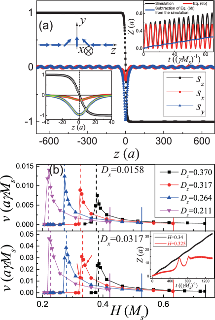
Figure 1: (Color online) (a) Schematic diagram of a 1D head-to-head DW (top-left inset) and the snapshot of $\mathbf{s}$ components at $t=200$ for $\alpha=0$, $J=53.7$, $D_{z}=0.317$, $D_{z}/D_{x}=10$ and $H=0.5$. Lower-left inset: the $\mathbf{s}$ profile of DW. Symbols are numerical results, vertical dashed line indicates the DW center position at $z=0.9$, and solid lines are Walker profile (4) with $\phi=Ht$ and $Z=0.9$. Right inset: the simulated motion evolution of DW center (black curve), the time dependence of DW center by collective coordinate model (red curve) and their difference (blue curve). (b) The field dependence of average DW speed $v$ for different $D_{z}$ and $D_{x}$. Vertical dashed and solid lines correspond to critical fields $H_{c1}$ and $H_{c2}$, respectively. Inset: simulated DW center for fields below and above $H_{c1}$ (indicated by arrows in the main figure).

In this section, we focus on a wire with a broad DW ($J/D_{z}\gg 1$) and a low transverse anisotropy $D_{z}/D_{x}\gg 1$. We first consider the dissipationless case ($\alpha=0$) with $J=53.7$ (YIG parameter YIG ), $D_{z}=0.317$ and $D_{z}/D_{x}=10$. The snapshot of spin profile near DW center at $t=200$ is shown in Fig. 1(a) when a field of $H=0.5$ is applied at $t=0$. Initially, the spin profile follows the well-known Walker solution Walker ; Yanpeng ; wieser ,

$$\theta_{n}=2\arctan e^{\frac{n}{\sqrt{J/(2D_{z})}}},\qquad\phi_{n}=\frac{\pi}{2},$$ (3)

with the DW width $\Delta=\sqrt{J/(2D_{z})}$. $\theta_{n}$, $\phi_{n}$ are polar angle and azimuthal angle of spin at site $n$. The DW emits SWs to both sides after the field is applied. The time dependence of the DW center $Z$, defined as the location where the spin has zero $z$-component, is shown in the right inset of Fig. 1(a). The DW plane precesses with frequency $H$ while DW center $Z$ oscillates periodically with frequency $2H$ and moves slowly and simultaneously along the field direction. The oscillatory DW motion can easily be explained by energy dissipation theory xrw though it is widely understood by the well known collective coordinate model suhl ; szhang ; tatara ; tatara1 , in which the DW is assumed to have a constant azimuthal angle $\phi(t)$ (no twisting). The polar angle $\theta_{n}(t)$, with DW width $\Delta{(t)}$, follows the Walker form

$$\begin{split}\theta_{n}(t)=2\arctan\exp\frac{n-Z(t)}{\Delta(t)},\\ \Delta(t)=\sqrt{\frac{J}{2[D_{z}+D_{x}\cos^{2}\phi(t)]}}.\end{split}$$ (4)

The DW dynamics is described by $\phi(t)$ and $Z(t)$,

$$\begin{gathered}\frac{d\phi(t)}{dt}+\frac{\alpha}{\Delta(t)}\frac{dZ(t)}{dt}=H,\\ -2D_{x}\sin\phi(t)\cos\phi(t)=\frac{1}{\Delta(t)}\frac{dZ(t)}{dt}-\alpha\frac{d\phi(t)}{dt}.\end{gathered}$$ (5)

When $\alpha=0$, the solution of Eq. (5) is

$$\phi=Ht,$$ (6a)

$$Z=2\frac{\sqrt{2JD_{z}}}{H}[\sqrt{1+\frac{D_{x}}{D_{z}}}-\sqrt{1+\frac{D_{x}}{D_{z}}\cos^{2}(Ht)}].$$ (6b)

Obviously, this is an exact solution of Eq. (2) only when $D_{x}=0$. It cannot describe the SW emission and the slow DW center propagation. The lower-left inset of Fig. 1(a) shows the spin profile from simulations (symbols) and from the collective coordinate model (solid curves) of Eqs. (4) and (6a) at $t=200$, with $Z=0.9$ instead of $0.29$ by Eq. (6b). One can see the spin profile near the DW center nevertheless follows Eqs. (4) and (6a) extremely well. Therefore, the DW width follows $\Delta{(t)}=\sqrt{J/2[D_{z}+D_{x}\cos^{2}\phi(t)]}$, a breathing motion with frequency $2H$. As shown in the right inset of Fig. 1(a), one can obtain the “pure” DW center propagation by subtracting Eq. (6b) (red curve) from numerically obtained $Z(t)$ (black curve). The results are plotted as the blue curve that is almost linear whose slope gives the average DW speed.

The field dependence of the average DW speed is shown in Fig. 1(b). Two critical fields $H_{c1}$ and $H_{c2}$ appear. In a field larger than $H_{c2}=2D_{z}$, there is no well-defined DW motion because the domain antiparallel to the applied field becomes unstable (the total effective field in the right domain is $(H-2D_{z})\hat{z}$ that is opposite to the spin direction when $H>2D_{z}$). Below $H_{c2}$, the domain is stable and so is the DW. As the field decreases, the average DW speed, though low, increases and increases rapidly before reaching $H_{c1}$. In the inset of Fig. 1(b), the time dependence of DW center position is shown for various fields below and above $H_{c1}$. Below $H_{c1}$, the DW propagation and SW emission become irregular, and the average DW speed is very low. Our discussion focus in the region of $H_{c1}<H<H_{c2}$.

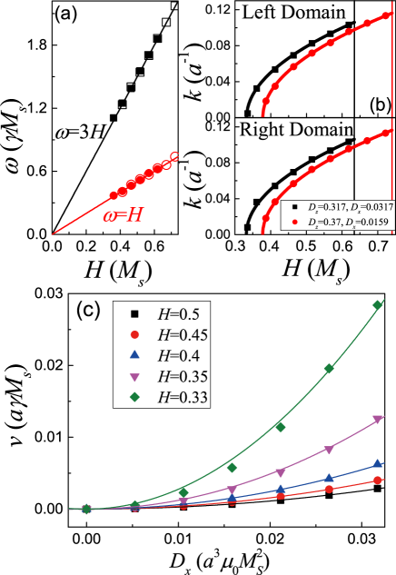
Figure 2: (Color online) (a) SW frequency $\omega$ as a function of applied field $H$. $\omega$ of the left domain is denoted by squares and that of the right domain by circles. Filled (open) symbols are results for $D_{z}=0.317$ and $D_{x}=0.0317$ ($D_{z}=0.37$ and $D_{x}=0.0158$). (b) SW wave number $k$ as a function of $H$. Upper (lower) part is for the left (right) domain. Solid curves are analytical results of Eq. (7) with $\omega_{+}=3H$ (upper) and $\omega_{-}=H$ (lower). Vertical lines indicate critical field $H_{c2}$. (c) Symbols are $D_{x}$ dependence of average DW speed for $D_{z}=0.317$ and various $H$. Solid curves are parabolic fits to the data.

In order to understand the mechanism of SW emission, we analyze the wave number $k$ and frequency $\omega$ from the Fourier transforms of the spatial distributions of $s_{i}$ (i=x,y,z) at a fixed time and the time dependence of a spin at a chosen point. The field dependence of SW frequency is plotted in Fig. 2(a) for a spin at $n=-100$ (left domain) and $n=100$ (right domain), for several different $D_{x}$ and $D_{z}$. The solid lines are $\omega=3H$ and $\omega=H$. The frequency in the left domain ($n=-100$) is close to $3H$ and that in the right domain ($n=100$) is close to $H$, independent of $D_{x}$ and $D_{z}$. The SW has good monochromaticity when $D_{x}/D_{z}\ll 1$, and the monochromaticity gradually degrades as $D_{x}/D_{z}$ increases. Following Wieser et al. wieser , the dispersion relation of SW can be obtained from Eq. (2) by small fluctuation expansion,

$$\begin{split}\omega_{\pm}(k)=&\sqrt{2J(1-\cos k)+2D_{z}\pm H}\\ &\times\sqrt{2J(1-\cos k)+2D_{z}+2D_{x}\pm H},\end{split}$$ (7)

where “+” and “-” are respectively for the left and the right domains. The wave number $k$ in the left and the right domains can then be uniquely determined by $3H=\omega_{+}(k)$ and $H=\omega_{-}(k)$, respectively. This relation is well verified by the numerical results shown in Fig. 2(b). The upper (lower) part is the field dependence of $k$ for the left (right) domain. The solid curves are analytical results Eq. (7). All numerical data (symbols) fall on the analytical curves. The spectrum is gapped with the minimal frequency $\omega_{0}=\sqrt{(2D_{z}\pm H)(2D_{z}+2D_{x}\pm H)}$. According to the early discussion, the DW precesses counter-clockwisely around $z$-axis at frequency $H$ and DW width breathes at frequency $2H$. It has already been shown that the breathing of DW width can emit SWs WXS and the generated SWs have the same frequency as that of the breathing. Thus, in the rotating frame of DW, the DW breathing emits SWs of frequency $2H$ to both sides. Because the SW in the left (right) domain is the collective spin procession motion in which spins precess counter-clockwisely (clockwisely) around the $z$-axis with frequency $2H$, the spin precession frequency in the left (right) domain is $2H+H=3H$ ($2H-H=H$) in the laboratory frame. To emit monochromatic SWs to both sides of the DW, spin precession frequencies on the left and right domains should match with the SW spectrum Eq. (7) that has a gap of $\sqrt{(2D_{z}\pm H)(2D_{z}+2D_{x}\pm H)}$. Thus $H_{c1}$ should be the larger $H$ satisfying $3H=\sqrt{(2D_{z}+H)(2D_{z}+2D_{x}+H)}$ and $H=\sqrt{(2D_{z}-H)(2D_{z}+2D_{x}-H)}$. When $D_{x}\ll D_{z}$ as used here, we have $H_{c1}\approx D_{z}+D_{x}/2$ which are shown by the vertical dashed lines in Fig. 2(b), and they agree with the numerical results well. This is called “breathing motion” because DW breathing is the origin of SW emission. SW emission can still occur below $H_{c1}$ but the emitted SWs are non-monochromatic because individual spin precession cannot be synchronized. Both the SW pattern and DW motion become complicated and irregular.

The average DW speed $v$ as a function of transverse anisotropy $D_{x}$ in a fixed field is shown in Fig. 2(c). When $D_{x}=0$, Eq. (6b) is the exact solution, and no DW breathing or SW emission can occur. The average DW speed is zero. As $D_{x}$ increases, $v$ increases rapidly. Numerical data can be fit by a parabolic function $v=CD_{x}^{2}$ (solid curves). The fitting is better for $H$ far above $H_{c1}$, and becomes worse (green curve) for $H$ close to $H_{c1}$.

The similar simulations were repeated for non-zero damping of $\alpha=0.001$ (reasonable for permalloy but $1\sim 2$ orders of magnitude higher than that of YIG). The snapshots of spatial distributions of three spin components at $t=200$ is shown in Fig. 3 with the same parameters as those in Fig. 1(a) except $\alpha$. The right inset is the time dependence of DW center position $Z(t)$ from numerical simulations (black curve) and theoretical prediction from Eq. (5) (red curve). The deviation is due to the SW emission and resulted DW propagation. The SW pattern is qualitatively the same as that of zero damping case except the decay of SW amplitude. The nice DW breathing motion and SW emission exist clearly in the presence of damping. Because of the energy conservation xrw ; WXS , the average DW speed connects directly to the SW emission power density $P$ by $P=2Hv$. Thus, Figs. 2(b) and (c) give also $H$ and $D_{x}$ dependences of $P$ with a proper factor of $2H$

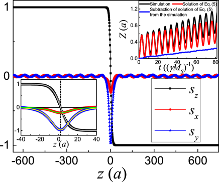
Figure 3: (Color online) Snapshot of $\mathbf{s}$ components at $t=200$ for $J=53.7$, $D_{z}=0.317$, $D_{z}/D_{x}=10$, $H=0.5$ and $\alpha=0.001$. Left inset: $\mathbf{s}$ profile of DW. Symbols are numerical results. Vertical dashed line indicates the DW center position at $z=2$, and solid curves are Walker profile (4) with $\phi=Ht$ and $Z=2$. Right inset: $Z(t)$ vs $t$ from simulations (black curve) and from solution of the collective coordinate model Eq. (5) (red curve). The difference (blue curve) shows the extra DW propagation due to SW emission.

III Drilling Motion

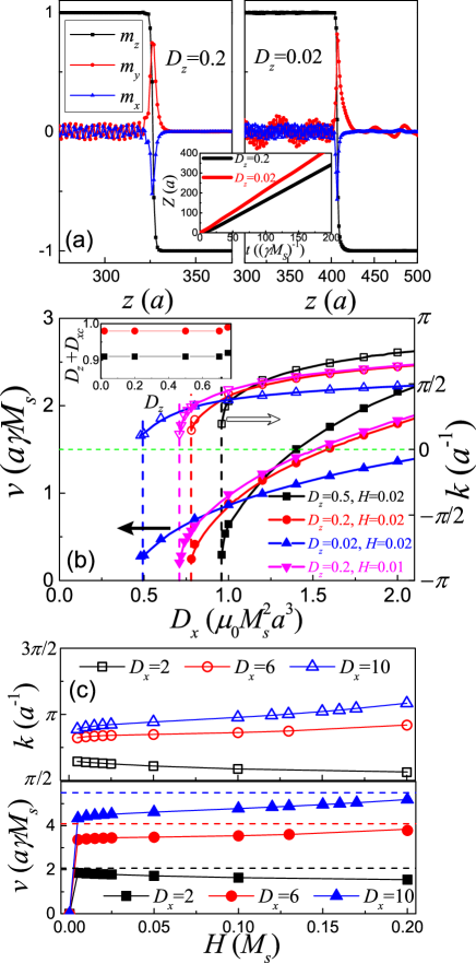
Figure 4: (Color online) (a) Snapshot of three spin components at $t=200$ for $J=2$, $D_{x}=2$, $\alpha=0$, $H=0.02$ and $D_{z}=0.2$ (left panel) or $D_{z}=0.02$ (right panel). Inset: Time-dependence of the DW center position for $D_{z}=0.2$ (black line) or $D_{z}=0.02$ (red line). (b) DW speed $v$ (left axis) and SW wave number $k$ in left domain (right axis) as a function of transverse anisotropy $D_{x}$. The dashed lines indicate the smallest $D_{x}$ for drilling motion. Inset: $D_{z}$ dependence of $D_{z}+D_{xc}$ for $H=0.02$ (red circles) and $H=0.01$ (black squares). The unit is $\mu_{0}M_{s}^{2}a^{3}$. (c) $k$ (upper panel) and $v$ (lower panel) as a function of applied field $H$ for $D_{z}=0.2$. The dashed lines indicate the largest speed from Eq. (5).

Fig. 4(a) is the snapshot of spatial distributions of three spin components at $t=200$ for $J=2$, $D_{x}=2$, $\alpha=0$, $H=0.02$ and $D_{z}=0.2$ (left panel) or $D_{z}=0.02$ (right panel). This wire has a strong hard axis ($D_{x}\gg D_{z}$). The wavy patterns away from the DW region are the emitted SWs. When $D_{z}=0.2$ only stern waves were observed while there are both bow and stern waves in the case of $D_{z}=0.02$. However, the stern waves are much bigger than the bow waves. The time dependence of DW center position is shown in the inset. The linear feature indicates a constant speed of DW propagation, completely different from the prediction of collective coordinate model. The azimuthal angle $\phi$ of the spins near the DW center is not a constant, meaning that the DW is distorted. The distortion comes from complicated misalignments of spins and their local effective fields under an external field and a high transverse anisotropy. Furthermore, $\phi$ angle at DW center does not rotate WXS . The DW emits SWs and moves forward like a drill.

The dependence of DW speed $v$ on transverse anisotropy $D_{x}$ is shown in Fig. 4(b) (left axis). There is a threshold $D_{xc}$ above which the drilling motion was observed. $v$ increases rapidly with $D_{x}$ near but above $D_{xc}$ and the incremental rate slows down for larger $D_{x}$. In order to find out the necessary condition for the drilling motion, simulations with different fixed $D_{z}$ and $H$ were carried out. $D_{xc}$ increases with $H$ for a fixed $D_{z}$. For a fixed $H$, the value of $D_{z}+D_{xc}$ is almost independent on $D_{z}$, as shown in the inset of Fig. 4(b). This indicates that the sum of the longitudinal and transverse anisotropies $D_{z}+D_{x}$ determines the drilling motion, instead of ratio $D_{x}/D_{z}$ conjectured in previous publications WXS ; wieser . A DW undergoes a drilling motion only when $D_{z}+D_{x}$ is close to $J$. Since DW width is of order of $\sqrt{\frac{J}{2(D_{z}+D_{x})}}$, this means that DW drilling motion appears when DW width approaches the lattice constant. This can be seen in Fig. 4(a) where $s_{z}$ varies from 1 to -1 within a few lattice sites. Thus, the motion of the DW can be described as follows: When a longitudinal field is applied to a static DW, the spins inside the DW experience a torque and rotate around $z$-axis, resulting in a finite component along hard axis ($x$-axis) and contraction of DW width. The strongly disturbed DW starts to emit SWs, and, as a consequence of energy conservation xrw , the DW has to propagate at a constant speed to release the Zeeman energy to compensate the energy carried away by SWs.

The DW speed $v$ shows a complicated dependence on applied field $H$, as shown in Fig. 4(c) (lower part). The DW speed $v$ jumps to a high speed at a very weak field. For a very large $D_{x}$, $v$ increases slowly with $H$. However, for a smaller $D_{x}$, $v$ decreases with $H$. Although the DW is twisted and the collective coordinate model completely fails in the drilling motion, the DW speed cannot exceed the largest speed predicted by Eq. (5), which ($\alpha=0$) is

$$v_{m}=\sqrt{2J}\sqrt{(D_{x}+2D_{z})-2\sqrt{D_{z}(D_{z}+D_{x})}},$$ (8)

(dashed lines in Fig. 4(c)). Interestingly, $v_{m}$ is also the maximal velocity of well-known solitons existing at $\alpha=0$ and $H=0$. A critical field $H_{c}=2D_{z}$ also exists in drilling motion for the same reason discussed in breathing motion. The dependence of wave number $k$ on $D_{x}$ and $H$ is shown in Figs. 4(b) (right axis) and 4(c) (upper panel), respectively, with the same trend as that of $v$. The wave number can be as large as $\pi$, indicating that shot wave with wavelength comparable to the lattice constant can be emitted. The dispersion relation Eq. (7) is verified by the numerical results.

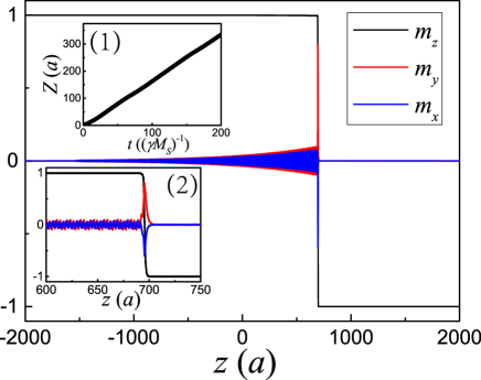
Figure 5: (Color online) Snapshot of spatial distributions of spin components at $t=200$ with $J=2$, $D_{z}=0.2$, $D_{x}=2$, $\alpha=0.001$ and $H=0.05$. Inset (1): The time dependence of DW center position. Inset (2): Enlarged figure near the DW center.

Fig. 5 is the snapshot of spatial distributions of $s_{x}$, $s_{y}$ and $s_{z}$ at $t=200$ with the same parameters as those in Fig. 4(a) except $\alpha=0.001$ and $H=0.05$. The Walker solution Walker doesn’t exist since $H>H_{W}\equiv\alpha D_{x}$. The DW still propagates at a constant speed while SWs are emitted. The spatially decaying pattern is due to the non-zero $\alpha$. The energy dissipation is through both the SW emission and the Gilbert damping. Clearly, the drilling motion with emission of SWs exists irrespective of the presence of the Gilbert damping or not.

Our numerical results show that the drilling motion may relate to strong twisting of DWs, to atomic scale, that may fail the continuum description of LLG equation Walker ; tatara ; tatara1 . Thus, our discussions do not apply $D_{z}$ close to or larger than $J$ because the static DW width would be of atomic scale. All initial DW configurations in our simulations follow the Walker profile well. A broad DW shrinks a little by a low transverse anisotropy, the DW undergoes a breathing motion. A high transverse anisotropy distorts the DW to an atomistic scale, and the drilling motion takes over DW dynamics. The average DW speed in breathing motion is quite low. Using YIG parameters $M_{s}=1.94\times 10^{5}$ A/m, $\gamma=28$ GHz/T and $a=1.23$ nm, the DW motion shown in Fig. 3 has a speed of 6 cm/s. The total SW emission power density per unit cross-section area is $P=2vH=2.8$ kW/m². DW speed in drilling motion is much higher. The estimated average speed is 132 m/s for YIG parameters and $D_{z}=0.1J$, $D_{x}=0.5J$ and $H=0.02J$. The total SW emission power is $2.5\times 10^{2}$ kW/m². For a nanoscale magnetic wire, the power can be of order of pW which is applicable in devices such as logic circuits KLWang . However, the anisotropy values used in this work are not realistic, at least for YIG because the crystalline anisotropy of YIG is about $0.02$ and the hard-axis shape anisotropy of a film is 0.5, which are much small than $J=53.7$. So in order to experimentally study the drilling motion, the material has to have high crystalline anisotropy and/or large saturation magnetization, and relatively weak exchange stiffness. All of our simulations were done by using oommf oommf and MuMax mumax that agree with each other well. Although SW emission is discussed in the context of energy dissipation and DW motion as a consequence of the energy dissipation WXS ; xrw , there are many other aspects about the interaction between DWs and SWs. For example, as discussed by Y. Le Maho et al. maho , an effective Gilbert damping constant was defined there due to SW emission. A modified damping constant can also modify a DW motion. The interaction between DWs and SWs may lead to a modification of the domain wall width and an effectively defined mass.

IV Conclusions

We numerically investigated the SW emission in field-driven DW motion. Two modes, breathing motion and drilling motion, were identified. In strong field and low transverse anisotropy, a broad DW undergoes a breathing motion. Both bow and stern SWs are emitted by the periodical breathing of DW width. The main frequencies of the SWs are $3H$ and $H$ in the domains along and opposite to the field, respectively. There is a lower critical field $H_{c1}$, due to the gap of SW spectrum, above which monochromatic SW is emitted. Only long wave can be emitted because applied field is limited by an upper critical value $H_{c2}$. The monochromaticity of the SWs degrades when the field decreases and/or the transverse anisotropy increases. When the sum of longitudinal and transverse anisotropy energies is of the same order of the exchange energy, the DW goes into drilling motion when DW plane is greatly distorted. The DW propagates at a constant high speed, and stern waves are mainly emitted. The SW wave number and DW speed increase with transverse anisotropy, and their field dependence is very complicated. The wavelength of the emitted SW can be very short (close to the lattice constant). Both breathing and drilling motion are robust against the presence of the Gilbert damping. The dispersion relation of the emitted SWs follows the theoretical formula.

V ACKNOWLEDGEMENTS

This work was supported by the NSF of China grant (11374249) and Hong Kong RGC grant (605413).

References

- (1) S.S.P. Parkin, M. Hayashi, and L. Thomas, Science 320, 190 (2008).
- (2) D.A. Allwood, G. Xiong, C.C. Faulkner, D. Atkinson, D. Petit, and R.P. Cowburn, Science 309, 1688 (2005).
- (3) G. Malinowski, O. Boulle, and M. Kläui, J. Phys. D: Appl. Phys. 44, 384005 (2011); C.H. Marrows and G. Meier, J. Phys.: Condens. Matter 24, 020301 (2012); G. Tatara, H. Kohno, and J. Shibata, Phys. Rep. 468, 213 (2008).
- (4) N.L. Schryer and L.R. Walker, J. Appl. Phys. 45, 5406 (1974).
- (5) A. A. Thiele, Phys. Rev. B 7, 391 (1973).
- (6) P. Yan, X. S. Wang, and X. R. Wang, Phys. Rev. Lett. 107, 177207 (2011).
- (7) D. Hinzke and U. Nowak, Phys. Rev. Lett. 107, 027205 (2011).
- (8) A. A. Kovalev and Y. Tserkovnyak, Europhys. Lett. 97, 67002 (2012).
- (9) X. S. Wang and X. R. Wang, Phys. Rev. B 90, 014414 (2014).
- (10) G. E. Khodenkov, Phys. Met. Metallogr. 107, 542 (2009).
- (11) R.Wieser, E.Y. Vedmedenko, and R.Wiesendanger, Phys. Rev. B 81, 024405 (2010).
- (12) M. Yan, C. Andreas, A. Kákay, F. García-Sánchez, and R. Hertel, Appl. Phys. Lett. 99, 122505 (2011).
- (13) X. S. Wang, P. Yan, Y. H. Shen, G. E.W. Bauer, and X. R. Wang, Phys. Rev. Lett. 109, 167209 (2012).
- (14) B. Hu and X. R. Wang, Phys. Rev. Lett. 111, 027205 (2013).
- (15) X.R. Wang, P. Yan, J. Lu and C. He, Ann. Phys. (N.Y.) 324, 1815 (2009); X.R. Wang, P. Yan, and J. Lu, Europhys. Lett. 86, 67001 (2009).
- (16) P. Yan and G. E.W. Bauer, Phys. Rev. Lett. 109, 087202 (2012).
- (17) D. Bouzidi and H. Suhl, Phys. Rev. Lett. 65, 2587 (1990).
- (18) G. Tatara and H. Kohno, Phys. Rev. Lett. 92, 086601 (2004).
- (19) J. Shibata, G. Tatara and H. Kohno, J. Phys. D: Appl. Phys. 44, 384004 (2011).
- (20) J. He and S. Zhang, Appl. Phys. Lett. 90, 142508 (2007).
- (21) A.A. Serga, A.V. Chumak and B. Hillebrands, J. Phys. D: Appl. Phys. 43, 264002 (2010).
- (22) Y. Le Maho, J.-V. Kim and G. Tatara, Phys. Rev. B 79, 174404 (2009).
- (23) A. Khitun, D. E. Nikonov and K. L. Wang, J. Appl. Phys. 106, 123909 (2009).
- (24) M. J. Donahue and D. G. Porter, National Institute of Standards and Technology Interagency Report No. NISTIR 6376, 1999.
- (25) A. Vansteenkiste and B. V. Wiele, J. Magn. Magn. Mater., 323, 2585 (2011).