Non-backtracking operator for Ising model and its application in attractor neural networks
Abstract
The non-backtracking operator was recently shown to give a redemption for spectral clustering in sparse graphs. In this paper we consider non-backtracking operator for Ising model on a general graph with a general coupling distribution by linearizing Belief Propagation algorithm at paramagnetic fixed-point. The spectrum of the operator is studied, the sharp edge of bulk and possible real eigenvalues outside the bulk are computed analytically as a function of couplings and temperature. We show the applications of the operator in attractor neural networks. At thermodynamic limit, our result recovers the phase boundaries of Hopfield model obtained by replica method. On single instances of Hopfield model, its eigenvectors can be used to retrieve all patterns simultaneously. We also give an example on how to control the neural networks, i.e. making network more sparse while keeping patterns stable, using the non-backtracking operator and matrix perturbation theory.
I Introduction
Ising model, which consists of spins arranged in a graph, is a fundamental model in statistical physics. It also has direct applications in many fields of science including e.g. physics Simon (1993); Mézard et al. (1987), neuron science Schneidman et al. (2006), computer science Hopfield (1982); Ackley et al. (1985) and social science Castellano et al. (2009). With different distribution of couplings, Ising model can act as model of different systems e.g. ferromagnets, spin glasses and neural networks. It gives a simple example of phase transitions, which is a phenomenon appearing in different fields of science, and it can be seen as a simple model for collaborative behavior of iterating systems.
Exact solution of Ising model only exists in special cases of topologies, e.g. one dimensional and two dimensional lattices. On a general graphs that the most applications meet, one usually needs approximations, especially with a general distribution of couplings. Commonly used approximations in statistical physics includes naïve mean-field approximation, TAP approximation and Kikuchi expansions. Among those approximation, one of the most popular approximation is Bethe approximation which assumes independence of conditional probabilities. Bethe approximation is exact on trees, and is found to be a good approximation on (random) sparse systems. Message passing algorithms based on Bethe approximation, so called Belief Propagation (BP) algorithms and its variations, have been used widely in many fields Mezard and Montanari (2009).
It has been recently proposed in Krzakala et al. (2013) that in network clustering (community detection) problem, where the task is to cluster nodes of graph into groups, Belief Propagation Yedidia et al. (2001), known in statistical physics as the cavity method Mézard and Parisi (2001), can be approximated by spectral clustering using a matrix called “non-backtracking” matrix . The reason is that in the clustering problem where permutation symmetry holds, BP equation always has a “paramagnetic” fixed-point where every node takes equal probability in each group. Linearizing BP equation around this paramagnetic fixed-point results to a linearized version of BP which is equivalent to spectral clustering using non-backtracking matrix on the graph. Spectral clustering using “non-backtracking” improves significantly the performance of clustering over other matrices like random walk matrix and Laplacians, and gives a nature choice of number of groups in the graph. The reason for the improvement is that non-backtracking matrix of a graph as a good property that almost all its eigenvalues are confined by a disk in the complex plane, so the eigenvalues corresponding to community structure lay outside the disk and are easily distinguishable.
Since the key that relates BP and non-backtracking matrix is the “paramagnetic” fixed-point, it is natural to think that similar for graphs, there must be also a non-backtracking matrix for Ising model when Ising model has a paramagnetic phase at high temperature without external fields. So the main purpose of this paper is to study the non-backtracking operator to Ising model on a graph with a given distribution of couplings at a certain temperature, and study some properties on spectrum of the matrix. Unlike non-backtracking matrix in graphs, the non-backtracking matrix of Ising model is a function of couplings and temperature. In another sense we can think it as a non-backtracking matrix of a weighted graph. We also study the application of matrix with some special distribution of couplings where Ising model acts like spin glasses or associative memory. We show how to use spectrum of to detect phases and phase transitions in the thermodynamics limit of system as well as in single instance of small systems. We will also give an example on how to control the neural network using eigenvalues and eigenvector of .
The paper is organized as follows. Section II includes definitions of the non-backtracking matrix for Ising model, some properties of its spectrum for general couplings are computed. In Section III we give several examples on Ising model with specific coupling distributions , including ferromagnet, Sherrington-Kirkpatrick model and Viana-Bray model. We show that in the thermodynamic limit results obtained using non-backtracking matrix recover the known results of phase boundaries. In Section IV we consider Hopfield model as associative memory where some binary patterns are memorized. In thermodynamics limit we recover the phase boundaries obtained by replica method, it also allows one to determine number of patterns and retrieve all the patterns simultaneously. On single instances we show how to make a given network more sparse while keeping patterns memorized using non-backtracking matrix. We conclude in Section V.
II Non-backtracking operator for Ising model
As we introduced in the introduction, non-backtracking operator appears naturally in linearizing BP of inference of stochastic block model Krzakala et al. (2013), also in linearizing BP for modularity Zhang and Moore (2014). So we can do similar things: obtaining non-backtracking operator by linearizing BP equation of Ising model at paramagnetic fixed point.
We consider Ising model on a graph with spins, is used to denote a configuration, with and . Energy (Hamiltonian) of system with zero external field is pairwise:
Boltzmann distribution with inverse temperature reads
On a single instance of the graph, one can use belief propagation algorithm to study the marginals of the Boltzmann distribution. For Ising model, BP equation reads
| (1) |
where denotes “cavity” probability of taking value with spin removed from the graph, denotes neighbors of and
| (2) |
is the normalization.
When BP equation converges on a graph, one can compute marginals of a spin taking value using
| (3) |
where again is the normalization.
It is easy to see that for all cavity messages and all marginals is always a fixed point of BP. We call this fixed point “paramagnetic” fixed-point. We can write BP messages as deviations from this paramagnetic fixed point:
with
| (4) |
It is easy to check that derivatives of BP messages evaluated at paramagnetic fixed-point reads
| (5) |
Equation (4) is a linearized version of BP equation (1), and it is equivalent to the eigenvector problem of an operator that we call non-backtracking for Ising model:
| (6) |
which is defined on the directed edges of the graph, with weight on each directed edge. If we use to denote number of edges in the graph, then the size of is . Note that in right hand side of last equation, is the non-backtracking operator used in Krzakala et al. (2013) for clustering problem. In discussion of Krzakala et al. (2013) authors suggested a weighted non-backtracking matrix, and our matrix can be seen as such weighted non-backtracking matrix, with weight on each edge.
Following the technique used in Krzakala et al. (2013), the edge of bulk of eigenvalues of can be computed by the following inequality,
| (7) |
where denotes one eigenvalue, and there are such eigenvalues. Note that is contributed by paths connecting edge with distance -step away:
where denotes one such path and denotes edges belonging to path . When is large, and couplings are i.i.d. distributed, for each path we have
where average is taken over realizations of couplings, and there are such paths with denoting excess degree
By taking expectation we have
Then relation (7) can be written as
| (8) |
and it holds for any . Last equation tells us that almost all ’s eigenvalues are confined by a disk of radius in the complex plan, with
| (9) |
The disk containing almost all the eigenvalues means the density of eigenvalues
is non-zero inside the disk, and is zero outside the bulk. Note that there could be outlier eigenvalues outside the bulk with zero density.
There is another way to understand the edge of bulk, in the sense of noise propagation on trees: consider some random noise with mean and unit variance are put on the leaves of a tree; by iterating , the noise may be propagated to the root of the tree with non-vanishing variance, if Thus radius of disk tells us that random noise could make Edwards-Anderson order parameter Edwards and Anderson (1975) of the system finite, which is a sign showing that system is in the “spin glass” state, and replica symmetry is breaking. So tell us where is the spin glass state and its relative strength to other possible states. point is also known as the de Almeida-Thouless local stability condition de Almeida and Thouless (1978), the Kesten-Stigum bound Kesten and Stigum (1966a, b), or the threshold for census or robust reconstruction Mezard and Montanari (2009); Janson and Mossel (2004).
If there are real-eigenvalues outside the bulk, they may tell us other possible state of the system, which correspond to other BP solutions. For example, if all the couplings are positive, it is easy to see that there could be one positive eigenvalue associated with an eigenvector with most of its entries positive. We can approximately recover this eigenvector by the following scheme: assume the graph is a tree with all its nodes associated with spin , or equivalently on the edge associated with leaves of the tree .
By steps iterating of , we define an ferromagnetic “approximate” eigenvector as
| (10) |
If with the vector is still correlated with , the all-one vector on the leave, system has a ferromagnetic state where information is preserved during iterating. On a tree, last equation can be written as contribution of paths connecting edge and edge distance away:
| (11) |
where denotes edges belong to path , and there are such paths.
When and are large, if we assume the self-average property,
| (12) |
Eq. (11) can be written as
| (13) |
where is again taking average over realizations of couplings.
Iterating once gives
| (14) |
and the eigenvalue is
| (15) |
is indeed an eigenvector of if goes to zero when is large. In another words, is an eigenvector if the noise propagation is slower than propagation of information , that is , which asks the informative eigenvalue of ferromagnetic state out of the bulk. Besides the ferromagnetic eigenvalue, there could be other real-eigenvalues representing other states of the system. So the competition of real-eigenvalues and gives us the information of the phases and phase transitions of system.
We note that and have been already computed in Mooij et al. (2014), using a different technique. However authors in Mooij et al. (2014) did not claim or show the sharp edge of bulk of spectrum. Another reason that we keep the detailed computation of and in this paper is that we need the technique in Sec. IV to compute the spectrum of non-backtracking matrix of Hopfield neural networks.
III Examples on ferromagnet and spin glasses
In this section we apply the non-backtracking operator to Ising model with specific distributions of couplings. One aim is to see whether non-backtracking operator recovers the known results of phase transitions on those systems.
III.1 Ferromagnetic Ising model on random graphs
For first example we consider ferromagnetic Ising model, which has . If we consider ferromagnet on Erdős-Rényi random graphs where , result given by non-backtracking matrix would be quite accurate, due to the locally tree-like structure of the topology. From the analysis of last section, for this model we have
and
thus is always larger than with finite and . It means this system can never be in spin glass state, it has to be in either ferromagnetic state or paramagnetic. And at , which implies that at
| (16) |
system undergoes a transition from paramagnetic to ferromagnetic phase.
Note that can be expressed as
| (17) |
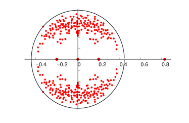
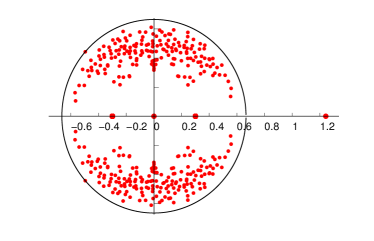
where is the non-backtracking matrix on the graph. From Krzakala et al. (2013) we know that has the largest eigenvalue , so as a sanity check, one can verify that . In Fig. 1 spectrum of is plotted in the complex plane for Ising model on a random graph with two values, one is in paramagnetic state and the other one is in ferromagnetic state. As shown in the figure, with , the largest eigenvalue of is smaller than one, which tells us that the paramagnetic fixed-point is stable. With , the largest eigenvalue of is greater than , telling us the paramagnetic fixed-point is unstable towards the direction of ferromagnetic state. It has been shown in Krzakala et al. (2013) that non-trivial part of ’s spectrum is can be obtained from a matrix
where is diagonal matrix with degree of nodes on the diagonal entries, is the identity matrix and is the adjacency matrix. Thus non-trivial part of ’s spectrum for ferromagnet can also be computed with less effort.
III.2 Ferromagnetic Ising model on networks with a community structure
If the network has a community structure, e.g. the number of edges connecting same group is much larger than number of edges connecting to different groups, besides the eigenvector pointing in direction to all-one vector, there could be other eigenvectors with some positive and some negative entries, with signs representing group memberships.
Here we consider networks that generated by a generative model named Stochastic Block Model (SBM) or planted partition model Decelle et al. (2011a, b). SBM is one of the widely used model to generate benchmark networks containing community structure. In the model, there are groups of nodes, each node has a pre-assigned group label , edges are generated independently according to a matrix by connecting each pair of nodes with probability . Here for simplicity we discuss the commonly studied case that matrix has only two distinct entries, if and if , and we use to denote the ratio between these two entries. A phase transition at Decelle et al. (2011a, b) has been discovered in this model that finite amount of information about planted partition can be inferred with , and one can do the optimal inference of SBM to recover information of all the way down to the transition. So it is a good benchmark for testing performance of community detection algorithms. Here we consider the simple two-group case with equal group sizes. From Krzakala et al. (2013) we know that in the detectable regime, edge of bulk of matrix is , it has two real eigenvalues outside the bulk, the first one corresponds to the eigenvector with entries having same sign. And the second one corresponds to the eigenvector correlated with community structure. According to Eq. (17), edge of bulk of matrix on the network is
first eigenvalue is , and the eigenvalue corresponding to the community structure is
So if , the community structure in the network is detectable by Ising model (by excluding the ferromagnetic state in some way).
Recall that Belief Propagation we used to derive the non-backtracking matrix at the beginning of the paper is nothing but an iterative method to decrease Bethe free energy; and a fixed point of Belief Propagation is a local minimum of Bethe free energy Yedidia et al. (2001). Obviously paramagnetic solution is always one local minimum of Bethe free energy. As we discussed above, eigenvalues larger than one in non-backtracking matrix tells us the instability of this paramagnetic fixed-point, which is also the instability of this local minimum of Bethe free energy. There is another way to study the instability of a minimum of free energy, which is Hessian matrix of Bethe free energy (we call it Hessian for simplicity) evaluated at paramagnetic fixed-point Saade et al. (2014); Ricci-Tersenghi (2012), which reads
| (18) |
Detailed derivations can be found at e.g. Ricci-Tersenghi (2012). For ferromagnets last equation reduces to
| (19) |
The paramagnetic state is stable if this matrix is positive semidefinite. If it has negative eigenvalues, there must be other minimums of free energy at some point in the phase space, in direction that pointed by components of eigenvectors corresponding to negative eigenvalues. This scheme has been used in Krzakala et al. (2013) to do spectral clustering on graphs where the Hessian is expressed as a function of , with in our settings.
Given and the graph, we have the following picture on the non-backtracking matrix and Hessian matrix: if , only paramagnetic fixed-point is stable, Hessian is positive semi-definite. If and , paramagnetic fixed-point is unstable towards the ferromagnetic state, Hessian has one negative eigenvalues. If , paramagnetic fixed-point is unstable towards both the ferromagnetic state and the planted configuration (the community structure), Hessian has two negative eigenvalues. Then we see that non-backtracking matrix works equivalently to Hessian in determine the phases of ferromagnets. But we note that computing spectrum of Hessian is much faster than non-backtracking matrix, because Hessian is symmetric and size of Hessian is smaller ( instead of in non-backtracking matrix).
If we are not interested in the phase of Ising model but only the problem of node clustering in a given network, we can choose as we want. As we shown above, does not influence the shape of spectrum of non-backtracking matrix, if , the second eigenvalue is always outside the bulk, thus we can always check whether there is a second eigenvalue outside the bulk to determine number of groups and use the eigenvector associated with it to detect the community structure. This is the idea explored in Krzakala et al. (2013) which uses matrix in doing spectral clustering.
The situation is different for Hessian, if is too small, Hessian is positive semidefinite, it looses its ability of determining number of groups in network. So it is important to select a good value that gives negative eigenvalues. The authors of Saade et al. (2014) suggested to chose , equivalent to set in our settings. As we discussed above, is the point that edge of bulk reaches , thus if there is a second real-eigenvalue of outside the bulk and is greater than , or equivalently a stable state correlated with community structure in Ising model, one should be able to find a second negative eigenvalue of with .
On the one hand, detecting number of groups using real eigenvalues of outside the bulk is easier than tunning value to look for negative eigenvalues of , especially on real-world networks. But on the other hand, tunning gives ability to optimize accuracy of detected communities, at least in synthetic networks.
III.3 SK model
Spin glass models were proposed to explain magnetic systems with frozen structural disorder, by introducing “frustration” using a particular distribution of couplings. Now theory of spin glasses e.g. replica symmetry breaking and cavity method find many application is many fields. In this section we consider non-backtracking matrix of two spin glass models, namely Sherrington-Kirkpatrick model Sherrington and Kirkpatrick (1975) and Viana-Bray model Viana and Bray (1985). It is well known that those spin glass models have paramagnetic phase at high temperature and spin-glass phase at low-temperature where both magnetization and Edwards-Anderson parameter are non-zero, and the replica symmetry is broken Mézard et al. (1987). First we consider Sherrington Kirkpatrick model which is defined on fully connected graph with couplings following Gaussian distribution:
From Eq. (9) and Eq. (15), we have
and
| (20) |
So the paramagnetic solution is stable as long as . And system enters spin glass state with . These are the well known results.
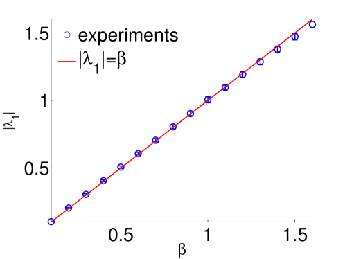
To test theory (Eq. (20)), in Fig. 2 we plot the edge of bulk (absolute value of the largest eigenvalues) as a function of for networks with . We can see that it consistent well with .
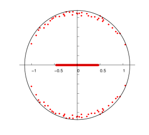
The spectrum of on SK model with two values are also shown in Fig. 3. We can see that with , the edge of bulk is smaller than , which means system is in paramagnetic phase. In the right ,with , the edge of bulk is greater than , system is in the spin glass phase. Moreover, from Eq. (15) we can also see that for the fully connected model distribution of couplings are not important, what really matters to the spin glass transition is the variance of couplings.
From the last section, we see that Hessian matrix of Bethe free energy works as well as non-backtracking matrix in detecting paramagnetic to ferromagnetic transition in ferromagnets, but it does not work well in SK model. Our numerical result (as well as experimental results in Mooij et al. (2014)) show that Hessian matrix for SK model is positive definite, thus it does not tell us where system encounters the spin glass transition.
III.4 Viana-Bray model
Viana-Bray model Viana and Bray (1985), also called model, is a spin glass model defined on random graphs. It is similar to the ferromagnets on random graphs but with couplings taking and randomly which give frustration to the system.
By varying and , the system can be in paramagnetic phase, spin glass phase or ferromagnetic phase. From Eq.(9)(15) we have
and
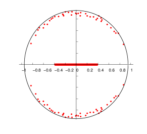
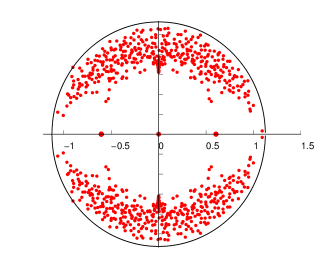
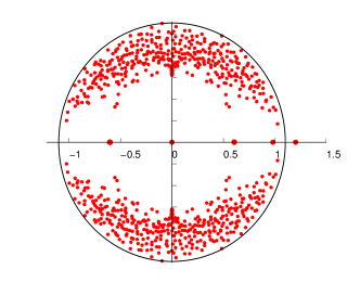
Obviously system undergoes paramagnetic to spin glass transition at independent of . And may undergo paramagnetic to ferromagnetic transition if . So our result recovers the phase boundaries derived using replica methods in Viana and Bray (1985). In Fig. 4 we plot the spectrum of non-backtracking matrix for Viana-Bray model in the complex plane for system in two phases, one in spin glass phase where there is no real eigenvalues outside the bulk, and the other one in ferromagnetic phase where there is one real eigenvalue outside the bulk and is greater than .
IV Non-backtracking operator for Hopfield model and controlling of neural networks
Hopfield model is a classic model for associative memory, it stores patterns by couplings of Ising model. We assume random binary patterns with , stored in network by Hebb’s rule Hebb (1949):
If patterns are memorized successfully, they can be retrieved by Glauber dynamics Glauber (1963): at time one neuron is randomly selected and its value is updated according to the probabilistic rule
From a random configuration, Glauber dynamics could converge to set of configurations that correlated with one pattern. If all patterns are memorized successfully in the network, each pattern will behave like an attractor to the Glauber dynamics, with different basin of attractions. That is why Hopfield model is categorized into attractor neural networks Amit (1992). The reason that patterns behave as attractors to the dynamics is that in Hebb’s rule, each pattern corresponds to a minima of free energy, and Glauber dynamics, which a “spin-flip” algorithm that converges to equilibrium, will trap into one of those local minimum of free energy.
The original Hopfield network was defined on fully-connected network, and its statistical mechanics has been studied Amit et al. (1985a, b) using replica method. However fully-connected model is not biologically realistic. In this paper we will focus on its more biologically-realistic version, which is Hopfield model on a random graph. The model is also called finite-connectivity Hopfield model and its statistical mechanics has also studied using replicas Wemmenhove and Coolen (2003), and phase boundaries were analyzed. The phase diagram of Hopfield model (both fully-connected and on a random graph) is composed of three parts: at high temperature every neuron behaves the same, magnetization is zero, system is in the paramagnetic phase; at a low temperature and with a low number of patterns, patterns are attractive to Glauber dynamics and system is in “retrieval” or “memory” phase; at a low temperature and a high number of patterns, network is confused by so many patterns thus none of the pattern is memorized successfully, Glauber dynamics will go away even started from one of the patterns, system is in spin glass phase.
Note that replica results were derived for the model at thermodynamic limit averaged over disorder (realizations of patterns), thus it is hard to apply the replica result to a single instance of network, to do tasks such as retrieving patterns and determining number of patterns. The classic way to do such tasks is Glauber dynamics. However on large networks it is time consuming, and the result depends on the initial configuration of the dynamics. And it is hard for Glauber dynamics to determine how many patterns stored in the network, because one can not explore all the initial configurations.
A faster way to retrieval patterns is running BP on the instance. But there is still a drawback that it is difficult to answer how many patterns there are in the network, since explore all possible initial messages for BP is hard.
In the rest part of the section we will study how to do the pattern retrieval task using non-backtracking matrix. It recovers replica result at thermodynamics limit easily, and on single instances it has advantages over Glauber dynamics and BP for speed as well as for determining number of patterns.
First we study the spectrum of non-backtracking operator at thermodynamic limit. From Eq. (9), the edge of bulk of Hopfield model, which tells us where is the spin glass phase, is expressed as
| (21) |
the averaging is taken over random patterns.
Obviously there is no stable “ferromagnetic” state since if we iterate with all-one configuration on leaves of the tree, we get
However, note that if instead of all-one configuration, we put a pattern in the leaves of the tree and do iterating, the information of the pattern could be preserved during iterating. It is very similar to initialize belief propagation by messages correlated with one pattern, or running Glauber dynamics from a pattern. Analysing iterating with a random pattern on leaves is difficult, but we can show it in an equivalent but easier way, by focusing on one of the stored patterns, let us say without loss of generality. Since patterns are chosen randomly and independently, we can do a gauge transformation to all the patterns which transforms to all-one configuration, and transforms other patterns to
It is easy to see that this transformation does not change distance between patterns, thus does not change the property of the system. Original patterns can be recovered easily by product again:
Under this transformation, couplings become
Obviously now couplings are biased to positive, and there could be a ferromagnetic state in the transformed system. Then we can treat term as a “signal” term that tells us information about all-one configuration, and term as a “noisy” term that gives some cross-talk noise to signal term. If there is only one pattern, cross-talk noise is , the problem essentially goes back to the ferromagnets. When number of pattern is small, noisy term has small fluctuation thus signal remains clear during iterating.
It is easy to see that the eigenvector correlated to the all-one vector in the transformed system is related to the eigenvector correlated with the first pattern in the original system. And the eigenvalue associated with the eigenvector correlated with all-one vector in the transformed system is the same with the eigenvalue associated with eigenvector correlated with first pattern in original system. With , this eigenvalue can be written as
| (22) |
So setting gives paramagnetic to retrieval transition and gives paramagnetic to spin glass transitions.
If we write last equation in the form of
| (23) | |||||
we can see that the expression for phase boundaries are in agreement with result obtained by replica method Wemmenhove and Coolen (2003), considering a little different definition of the model. Moreover, with patterns chosen randomly at thermodynamic limit, we have
| (24) |
If we do the above gauge transform on every pattern, we would have such eigenvalues. But note that though we studied the and with the gauge transform, it is only a trick to study analytically in an easier way the eigenvalues. In a single instance, we do not need to do such transform, there should be eigenvalues corresponds to patterns. And on the given network, once we find real eigenvalues outside the bulk, we can use eigenvectors associated with those eigenvalues to retrieve patterns.
For more detail, after we have an eigenvector , first we obtain the vector containing summation of incoming values from edges for nodes, from an eigenvector ,
Then we set positive entries of to and negative entries to , and zero entries to or randomly. The obtained configuration should be correlated with the pattern, i.e. the overlap parameter which is inner product of obtained configuration and a pattern
| (25) |
is positive.
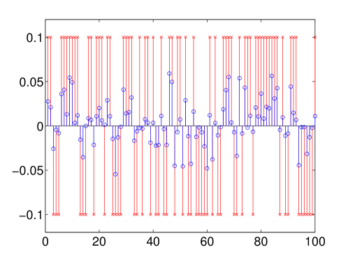
In Fig. 5 we plot one memorized binary pattern compared with one eigenvector of non-backtracking matrix, we can see that the sign of components of eigenvector are correlated with sign of the binary pattern.
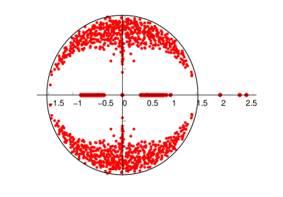
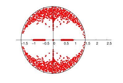
In Fig. 6 we plot the spectrum of a Hopfield network with different parameters in the complex plane. In left panel, , three patterns are memorized, system is in retrieval phase. There are three eigenvectors outside the edge of bulk, and the associated eigenvectors are correlated with three stored patterns, with the overlap (Eq.(25)) for three patterns much larger than . In right panel, , none of the patterns is memorized successfully. In spectrum, the edge of bulk is larger than , there is no real eigenvalues outside the bulk, so system is in spin glass state.
In the thermodynamic limit, self-averaging property will make those eigenvalues identical. But in the finite-size networks, we could obtain different eigenvalues, telling us that patterns are not memorized equally strong. One example is shown in left panel of Fig. 6 where three real-eigenvalues outside the bulk are not equal to each other. When real-eigenvalues are all out of bulk but not equal, though from random initial vectors, iterating will always leads to the eigenvector associated with the largest eigenvalue, other patterns could be retrievable by other methods, E.g. by running Glauber dynamics starting from a configuration or running BP from a random messages. We have tested that by running Glauber dynamics we can reach other patterns according to the eigenvalues outside the bulk from random initial configurations. We think the pattern with the largest eigenvalue are indeed stronger than other two patterns, and has larger basin of attraction than other two patterns; however its basin attraction does not dominate the entire configuration space, so other two patterns are still able to attract Glauber dynamics.
Another situation is that not all eigenvalues are outside the bulk and larger than . This means not all the patterns are memorized stably. We have tested that in this case only patterns according to eigenvalues outside the bulk are attractive to Glauber dynamics. For those patterns according to eigenvalues inside bulk or smaller than , Glauber dynamics starting from exactly the pattern will still run away and converge to configurations around other patterns. So those patterns are indeed not retrievable.
So as described above, we can find all real-eigenvalues and use all real-eigenvectors associated with those eigenvalues to retrieve pattern simultaneously, as opposed to BP or Glauber dynamics, where only one pattern is retrieved at one time, without knowing neither total number of patterns, nor which patterns are memorized stronger than the others.
Besides the phase diagram, another property that has been studied extensively in neural networks is the capacity of the network that we denote by . Capacity is the maximum number of patterns (divided by number of neurons) that could be stored successfully. This property is closely related to the strength of the memorized patterns. In our picture of spectrum of non-backtracking operator, by increasing number of patterns, number of real eigenvalues outside of bulk increases, but each of eigenvalue becomes closer to the bulk. When exceeds , real-eigenvalues disappear and become complex eigenvalues, then system enters spin glass phase and losses all the memory.
A large amount of studies have been devoted to increase capacity and the retrieval abilities of neural networks by optimizing the learning rule or by optimizing the topology of the network Anthony and Bartlett (2009); McGraw and Menzinger (2003); Kim (2004); Morelli et al. (2004); Zhang and Chen (2008a, b); Braunstein et al. (2011). In the following text of the paper we are going to discuss more on optimizing the topology of the network. We know that fully-connected Hopfield network can store number of patterns proportional to number of neurons, but the fully-connected topology is not biological realistic. On the other hand, when we dilute the network, i.e. by making the network more and more sparse by removing edges, number of patterns stored is decreasing but the number of patterns per edge is increasing Wemmenhove and Coolen (2003). Thus one interesting question would be, given a network, how to make the network more sparse while keeping information of pattern stored by the network unchanged. This problem could be studied easily by non-backtracking matrix, since real eigenvalues outside the bulk tell us the stability of patterns, if we can keep those eigenvalues unchanged in manipulating topology of the network, we can keep those patterns stable in the network. A nature idea to keep eigenvalues could be by converting the problem to an optimization problem that at each time we remove the edge that decrease least the gap of eigenvalues,
where is the eigenvalue corresponding to the pattern we want to keep, and is the edge of bulk of non-backtracking matrix. This process is easy to implement but the computation is time consuming because selecting the edge that decreases least the spectral gap we have to remove every edge from the graph one by one, compute eigenvalues, then add the edge back. One way to make the process faster is to remove the edge that changes least the spectral gap among small randomly selected subset of edges. Actually if we are interested in keeping one eigenvalue instead of keeping the gap, we can do things much easier.
Assume after one edge removed, matrix becomes
If we look as a perturbation to the matrix and assume that after the perturbation, an eigenvalue changes from to , a left eigenvalue changes from to , and a right eigenvector changes from to , then we have the following relation
Ignoring second order terms, we have
Multiplying left eigenvector in both sides of last equation results to
then the expression of change of by perturbation is written as:
| (26) |
In our problem is actually a matrix with entries zero except those with edges and involved. Then the last equation can be written as
| (27) | |||||
So the change of eigenvalues becomes a function of left and right eigenvectors. By computing once the eigenvectors, we know exactly which edge could change least the eigenvalue. So we can make network more sparse while keeping information of a pattern stable, by removing edges that give least iteratively. For more detail, at each step, left and right eigenvectors associated with a real eigenvalue are computed, one (or several edges) that minimizes are removed, then the above process are repeated until network is sparse enough. Note this procedure is similar to the decimation algorithm using marginals of a message passing algorithm in solving constraint satisfaction problems Mézard et al. (2002), where nodes having most biased marginals are removed (fixed) at each iterating.
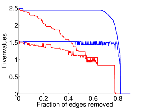
We did some numerical experiments on the edge-removing scheme and compared its performance with random removing in Fig 7, where the real eigenvalue and edge of bulk are plotted as a function of fraction of edges removed. We can see from the figure that random removing makes the real eigenvalue decreasing very fast while our process keep the eigenvalue unchanged up to more than half edges removed. Though edge of bulk in our process decreases also slower, the real eigenvalue joins bulk later than that in random removing.
Note that the problem of removing edges is just a simple example of optimizing topology of a neural network using the non-backtracking operator. Since information of stability of patterns can be obtained at same time by non-backtracking matrix we believe other kinds of topology optimization on neural networks can also be done easily using non-backtracking matrix.
V Conclusion and Discussions
As a conclusion, we have introduced non-backtracking operator for Ising model with general coupling distributions, it can be seen as a generalization of non-backtracking operator from a unweighted graph to weighted graph with an edge weighted by . In thermodynamic limit its spectrum gives us phase transitions of the model. And in single instances its eigenvectors can be used to control the model.
All above studies were made for Ising model without external fields. With external fields present, it has been shown Parisi et al. (2014) that paramagnetic solution still exists but with finite magnetization. It would be interesting to extend current study to that case.
If one compares the spectrum of non-backtracking operator of a Hopfield model with patterns and that of a network generated by stochastic block model with communities, one find that they are quite similar. However the stochastic block model corresponds to a Potts model with states and one basin of attraction, as opposed to Hopfield model which corresponds to Ising model with states and basin of attractions. So it would be interesting to study such connection in detail in future work.
Note that spectrum density of non-backtracking matrix of a graph has been computed in Saade et al. (2014) using Belief Propagation. It would be interesting to compute non-backtracking matrix of Ising model using the same technique.
Acknowledgements.
P.Z. was supported by AFOSR and DARPA under grant FA9550-12-1-0432. We are grateful to Ruben Andrist, Florent Krzakala, Cristopher Moore, Alaa Saade and Lenka Zdeborová for helpful conversations, and Federico Ricci-Tersenghi for discussing and pointing out reference Mooij et al. (2014); Parisi et al. (2014).References
- Simon (1993) B. Simon, The Statistical Mechanics of Lattice Gases, Volume I (Princeton University Press Princeton, New Jersey, 1993).
- Mézard et al. (1987) M. Mézard, G. Parisi, and M. Virasoro, Spin glass theorey and beyond (World Scientific, 1987).
- Schneidman et al. (2006) E. Schneidman, M. J. Berry, R. Segev, and W. Bialek, Nature 440, 1007 (2006).
- Hopfield (1982) J. J. Hopfield, Proc. Natl. Acad. Sci. USA 79, 2554 (1982).
- Ackley et al. (1985) D. H. Ackley, G. E. Hinton, and T. J. Sejnowski, Cognitive Science 9, 147 (1985), ISSN 0364-0213, URL http://www.sciencedirect.com/science/article/pii/S0364021385800124.
- Castellano et al. (2009) C. Castellano, S. Fortunato, and V. Loreto, Reviews of modern physics 81, 591 (2009).
- Mezard and Montanari (2009) M. Mezard and A. Montanari, Information, Physics and Computation (Oxford University press, 2009). J. Yedidia, W. Freeman, and Y. Weiss, in International Joint Conference on Artificial Intelligence (IJCAI) (2001
- Yedidia et al. (2001) J. Yedidia, W. Freeman, and Y. Weiss, Exploring artificial intelligence in the new millennium 8, 236 (2003).
- Krzakala et al. (2013) F. Krzakala, C. Moore, E. Mossel, J. Neeman, A. Sly, L. Zdeborová, and P. Zhang, Proc. Natl. Acad. Sci. USA 110, 20935 (2013), eprint http://www.pnas.org/content/110/52/20935.full.pdf+html, URL http://www.pnas.org/content/110/52/20935.abstract.
- Yedidia et al. (2001) J. Yedidia, W. Freeman, and Y. Weiss, in International Joint Conference on Artificial Intelligence (IJCAI) (2001).
- Mézard and Parisi (2001) M. Mézard and G. Parisi, Eur. Phys. J. B 20, 217 (2001).
- Zhang and Moore (2014) P. Zhang and C. Moore, arXiv preprint arXiv:1403.5787 (2014).
- Edwards and Anderson (1975) S. Edwards and P. Anderson, J. Phys. F 5, 965 (1975).
- de Almeida and Thouless (1978) J. R. L. de Almeida and D. J. Thouless, J. Phys. A 11, 983 (1978).
- Kesten and Stigum (1966a) H. Kesten and B. P. Stigum, The Annals of Mathematical Statistics 37, 1211 (1966a).
- Kesten and Stigum (1966b) H. Kesten and B. P. Stigum, The Annals of Mathematical Statistics 37, 1463 (1966b).
- Janson and Mossel (2004) S. Janson and E. Mossel, Annals of probability pp. 2630–2649 (2004).
- Decelle et al. (2011a) A. Decelle, F. Krzakala, C. Moore, and L. Zdeborová, Phys. Rev. E 84, 066106 (2011a), URL http://link.aps.org/doi/10.1103/PhysRevE.84.066106.
- Decelle et al. (2011b) A. Decelle, F. Krzakala, C. Moore, and L. Zdeborová, Phys. Rev. Lett. 107, 065701 (2011b), URL http://link.aps.org/doi/10.1103/PhysRevLett.107.065701.
- Saade et al. (2014) A. Saade, F. Krzakala, and L. Zdeborová, arXiv preprint arXiv:1406.1880 (2014).
- Ricci-Tersenghi (2012) F. Ricci-Tersenghi, J. Stat. Mech. 2012, P08015 (2012), URL http://stacks.iop.org/1742-5468/2012/i=08/a=P08015.
- Sherrington and Kirkpatrick (1975) D. Sherrington and S. Kirkpatrick, Phys. Rev. Lett 35, 1792 (1975).
- Viana and Bray (1985) L. Viana and A. Bray, J. Phys. C 18, 3037 (1985).
- Hebb (1949) D. O. Hebb, The organization of behavior: A neuropsychological approach (John Wiley & Sons, 1949).
- Glauber (1963) R. J. Glauber, Journal of Mathematical Physics 4, 294 (1963).
- Amit (1992) D. J. Amit, Modeling brain function: The world of attractor neural networks (Cambridge University Press, 1992).
- Amit et al. (1985a) D. Amit, H. Gutfreund, and H. Sompolinsky, Phys. Rev. Lett. 55, 1530 (1985a).
- Amit et al. (1985b) D. Amit, H. Gutfreund, and H. Sompolinsky, Phys. Rev. A 32, 1007 (1985b).
- Wemmenhove and Coolen (2003) B. Wemmenhove and A. Coolen, J. Phys. A: Math Gen. 36, 9617 (2003).
- Anthony and Bartlett (2009) M. Anthony and P. L. Bartlett, Neural network learning: Theoretical foundations (cambridge university press, 2009).
- McGraw and Menzinger (2003) P. N. McGraw and M. Menzinger, Phys. Rev. E 68, 047102 (2003).
- Kim (2004) B. J. Kim, Phys. Rev. E 69, 045101 (2004).
- Morelli et al. (2004) L. G. Morelli, G. Abramson, and M. N. Kuperman, Eur. Phys. J. B 38, 495 (2004).
- Zhang and Chen (2008a) P. Zhang and Y. Chen, Physica A 387, 4411 (2008a).
- Zhang and Chen (2008b) P. Zhang and Y. Chen, Physica A 387, 1009 (2008b).
- Braunstein et al. (2011) A. Braunstein, A. Ramezanpour, R. Zecchina, and P. Zhang, Phys. Rev. E 83, 056114 (2011).
- Mézard et al. (2002) M. Mézard, G. Parisi, and R. Zecchina, Science 297, 812 (2002).
- Saade et al. (2014) A. Saade, F. Krzakala, and L. Zdeborová, Europhysics Letters 107, 50005 (2014).
- Mooij et al. (2014) J. M. Mooij and H.J. Kappen, Journal of Statistical Mechanics: Theory and Experiment 2005, P11012 (2005).
- Parisi et al. (2014) G. Parisi, F. Ricci-Tersenghi, and T. Rizzo, Journal of Statistical Mechanics: Theory and Experiment 2014, P04013 (2014).