An Efficient Second-Order Accurate and Continuous Interpolation for Block-Adaptive Grids

Abstract

In this paper we present a second-order and continuous interpolation algorithm for cell-centered adaptive-mesh-refinement (AMR) grids. Continuity requirement poses a non-trivial problem at resolution changes. We develop a classification of the resolution changes, which allows us to employ efficient and simple linear interpolation in the majority of the computational domain. The benefit of such approach is higher efficiency. The algorithm is well suited for massively parallel computations. Our interpolation algorithm allows extracting jump-free interpolated data distribution along lines and surfaces within the computational domain. This capability is important for various applications, including kinetic particles tracking in three dimensional vector fields, visualization (i.e. surface extraction) and extracting variables along one-dimensional curves such as field lines, streamlines and satellite trajectories, etc. Particular examples of the latter are models for acceleration of solar energetic particles (SEPs) along magnetic field-lines. As such models are sensitive to sharp gradients and discontinuities the capability to interpolate the data from the AMR grid to be passed to the SEP model without producing false gradients numerically becomes crucial. The code implementation of our algorithm is publicly available as a Fortran 90 library.

1 Introduction

The adaptive-mesh-refinement (AMR) grids [1] have become an essential part of many applications in computational physics. The AMR is an effective technique which allows us to adapt grid to particular features being simulated. For example adaptive spatial discretization is employed by the Block-Adaptive Tree Solarwind Roe-type Upwind Scheme (BATS-R-US) code for solving MHD equations [2, 3, 4, 5], which is the heart of Space Weather Modeling Framework (SWMF) [6, 7, 8].

Often the physical quantities to be calculated are sampled at cell centers especially within the framework of control volume method. To obtain data at different locations one needs an interpolation algorithm. A high variety of approaches allows us to achieve the second order of accuracy. While for many applications this is enough to obtain accurate results, certain applications are sensitive to continuity, and therefore require an interpolation method that does not generate artificial discontinuities. For such cases an algorithm is needed, which meets requirements of both continuity and second order of accuracy.

A particular application that motivated us to develop such algorithm is acceleration of solar energetic particles (SEPs) at the shock wave fronts. The model presented in [9, 10, 11, 12] employs magnetic field line tracing as well as interpolation of solar wind parameters from the BATS-R-US AMR grid to the locations of the magnetic field lines points. Unphysical discontinuities within the interpolation algorithm affect results by producing particle acceleration/deceleration at false shocks near grid irregularities. Hence, the model’s reliability is crucially dependent on the continuity of interpolation algorithm.

The problem of AMR interpolation has a variety of possible applications, under which it has been addressed before [13, 14, 15, 16]. In the latter reference, the authors considered it in the context of the total-variation-diminishing (TVD) principle applied to block-adaptive grids. Interpolation is an important part of the limited reconstruction procedure, the choice of the interpolation algorithm affects stability and accuracy of a scheme it is being applied to. Another possible application is visualization of the result obtained in simulations with AMR grids. In this context the problem of continuous AMR interpolation has also been addressed [17, 18, 19]. Therefore, development of such algorithm is not a problem of merely mathematical interest but it is also of importance in applications.

The numerical results obtained by control volume method in conjunction with AMR are sampled on the cell-centered grid. To visualize data, one way is to resample them to corner-centered grid as done by many visualization tools, such as Tecplot. However, this approach involves more distant grid cells and, as a result, smoothens the data. Alternative way is to visualize the uniform parts of the AMR grid directly and to create a smooth transition between parts of the grid at different resolution levels. To do so in [17, 18, 19], the authors developed a stitching algorithm, as described in details in [17].

Their method achieves continuity and the second order of accuracy. Tessellation of the computational domain into simpler shapes is employed, and the interpolation procedure is fully defined by the geometry of a particular shape a given point falls into. The algorithm is easy to understand and, hence, simple to implement. However, when developing our algorithm, we focused on its efficiency. Compared to the stitching algorithm, it is advantageous in the sense that it uses the same simple interpolation procedure over large portion of the computational domain. As described further, the stitching algorithm is double-branched in two dimensions (2D) and triple-branched in 3D, while ours stays uniform. Therefore the latter is preferable for repeated interpolation during the simulation.

2 Grid specification

Here, we focus on block-adaptive AMR grids and assume that the computational domain is decomposed into blocks, each block being a rectangular box in Cartesian (or logically Cartesian) coordinates. The blocks are decomposed into $i\times j\times k$ “cells”, for three-dimensional (3D) case, the cell-per-block integer numbers (usually, even) being constant throughout the whole grid, which maintains the claimed blocks similarity. Being similar, the blocks, however, are not all identical, as long as the cell size in different blocks may differ. Specifically, we assume that in the neighboring blocks (having at least one common point on the boundary) the cell size, $\Delta x^{(C)},\,\Delta y^{(C)},\,\Delta z^{(C)}$, in the coarser (C) block may be by a factor of two larger than those in the finer (F) block:

$\Delta x^{(C)}=2\Delta x^{(F)},\,\Delta y^{(C)}=2\Delta y^{(F)},\,\Delta z^{(C)}=2\Delta z^{(F)}$.

Refinement ratios more than 2 are also possible and the algorithm generalizes to these cases, but our implementation is restricted to the refinement ratio of 2.

We assume that the numerical solution of the governing equations, obtained at each time step, is a cell-centered grid function, e.g. the solution obtained using control volume method. In order to find a numerical solution at an arbitrary point within the computational domain one needs to find the way to interpolate data from the cell-centered block-adaptive AMR grid. The goal of the present work is to find the procedure to interpolate data from cell-centered block-adaptive logically Cartesian AMR grid, which continuously connects bilinear interpolation from the uniform parts of the grid through the resolution changes.

Indeed, for a uniform 2D Cartesian grid the easiest and most natural approach is a bilinear interpolation (for three dimensions it is trilinear interpolation). It is efficient and of the second order accuracy. Another advantage is that type of interpolation retains symmetries with respect to the coordinate axes if they are assumed by a correspondent symmetry of the problem to be solved. Should one perform the interpolation by splitting the computational domain into a set of tetrahedra, the second order accuracy would be also achieved, however, the symmetry of the numerical solution will be broken, as long as the set of tetrahedra would not be symmetric. In addition, this partitioning is not a unique solution, thus making ambiguous the interpolation procedure. The latter may be unacceptable.

Compared to tetrahedron-based method trilinear interpolation has one important drawback: it is not continuous when directly applied near grid resolution changes. This requires us to generalize the trilinear interpolation method for these problematic sites, as we describe below.

3 Basic concepts and definitions

In this section we describe basic definitions and methodology. Many ideas naturally translate from lower to higher dimensions. For this reason notations have been developed in an arbitrary number of dimensions $N$.

For any arbitrary point X an algorithm solves two distinct problems: to determine an interpolation stencil (set of cells involved into interpolation with non-zero weights) and to calculate interpolation weights. An interpolation stencil should consist of cells that are close to X. In order to elucidate “closeness” we introduce the following notions.

Enclosing stencil for point X (the point X is enclosed by this stencil) is a set of $2^{N}$ grid cell centers with their coordinate vectors, $\mathbf{x}_{1}$, … , $\mathbf{x}_{2^{N}}$, satisfying the following two conditions:

First, the rectangular box bounded by their coordinates contains point $\mathbf{X}=(X,Y,Z)$. For example, for 2D grids cell centers in the enclosing stencils for point X must satisfy inequalities:

$$x_{1}\leq X<x_{2}, \hskip 20.0pty_{1}\leq Y<y_{3},$$

$$x_{3}\leq X<x_{4}, \hskip 20.0pty_{2}\leq Y<y_{4}.$$ (1)

In 3D case for the first four points, $\mathbf{x}_{1}$, .., $\mathbf{x}_{4}$, the inequalities (1) are fulfilled together with the requirement, $z_{i}\leq Z$, where $i=1,..,4$. For the last four points, $\mathbf{x}_{5}$, .., $\mathbf{x}_{8}$, the inequalities analogous to (1) are fulfilled together with the requirement, $Z<z_{i}$, where $i=5,..,8$.

Second, each edge of that box does not exceed the linear size of Coarser cells, $\Delta x^{(C)}$, $\Delta y^{(C)}$, along the corresponding axis, $i$, e.g. for 2D grids:

$$|x_{1,3}-x_{2,4}|\leq\Delta x^{(C)},$$

$$|y_{1,2}-y_{3,4}|\leq\Delta y^{(C)}.$$ (2)

As a part of definition, we introduce notion of Fine cluster. Two Finer grid points of the enclosing stencil form a 2-cluster, if they lay on a line parallel to a coordinate axis, while four Finer grid points form a 4-cluster, if they lay on a plane parallel to a coordinate plane, etc. To reduce an ambiguity, we set an extra constraint on an enclosing stencil, by claiming that the set of conditions (2) should be strict inequality for stencil points, e.g. 1 and 2, if both belong to the same Fine cluster, e.g. $|x_{1}-x_{2}|<\Delta x^{(C)}$. In this way we exclude from consideration the enclosing stencils, which unreasonably involve farther Finer grid points instead of closer ones.

Figure 1: Ambiguity of an enclosing stencil. All points inside the shaded rectangles are enclosed by 2 different stencils: (0,1,4,2) and (0,1,4,3) for dark gray, (0,1,3,2) and (0,1,4,2) for horizontal light gray, (0,1,4,3) and (0,2,4,3) for vertical light gray.

Still, we emphasize that an enclosing stencil is not unique for many point locations, as illustrated in Figure 1. For this reason it can’t be identified with an interpolation stencil, which must be unambiguous. However, all stencils enclosing the same point have the same values of edge type. Herewith, we say that a stencil has an edge type $n$, $n\leq N$, if it has resolution changes in $n$ dimensions. Within this approach, $(N{-}n)$-dimensional rectangles, which are shaped by points of a stencil parallel to the remaining dimensions, are refered to as trivial elements of this stencil. Interpolation procedure on them is a simple generalization of a linear interpolation.

We refer to a set of points satisfying (1) for a given enclosing stencil as an enclosed set of this stencil. An enclosed set is an $N$-dimensional rectangular box. Adjacent enclosed sets of enclosing stencils of the same edge type, $n$, merge together into a resolution n-edge. Particularly, 0-edge (i.e. no resolution change) is a closed isolated domain covered by a uniform Cartesian grid. The following easy-to-prove claims are important. First, any given point can belong to one and only one resolution edge. In other words, the computational domain decomposes into a set of resolution $n$-edges. Second, for $n<N$, one can use simple linear interpolation in all dimensions that do not have a resolution change, i.e. on trivial elements. Thus, the effective dimensionality of non-trivial interpolation procedure for $n$-edge reduces to $n$. Indeed, this non-trivial interpolation procedure should be introduced on an $n$-dimensional subspace orthogonal to trivial elements.

Therefore, we define a main interpolation subset for point X inside a resolution $n$-edge as a cross-section of this $n$-edge by $n$-dimensional plane that includes point X and is perpendicular to trivial elements of enclosing stencils for the point X. Particularly, for $n{=}N$ main interpolation subset coincides with the resolution $n$-edge itself. For 1-edge we refer to it as main interpolation line (see Figure 3), for 2-edge - main interpolation plane (see Figure 4).

As the last definition, an extended interpolation stencil for a point X is a minimal union of stencils enclosing together the main interpolation subset for this point. Unlike an enclosing stencil, the extended interpolation stencil is unique for any given point.

This gives us a starting point to outline the following algorithm. First, for a given point X we need to figure out the type of $n$-edge it belongs to. Based on found value of $n$ and point location, one needs: (1) to construct the extended interpolation stencil; (2) to choose the actual interpolation stencil from the extended interpolation stencil; and (3) to calculate the interpolation weights. Then, with grid points forming the interpolation stencil for X, indexed by $i=1,..,m$, interpolation weights, $w_{i}$, and values of a function $f$ sampled at grid points, $f_{i}$, the interpolated value in X is calculated as $f(\mathbf{X})=\sum_{i=1}^{m}{w_{i}f_{i}}$. We note that our algorithm does not use ghost cells. In a parallel implementation, the sum can be calculated with an MPI_reduce call, for example.

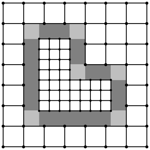
Figure 2: Stitching (see [17]) and resolution edges (white - 0-edges, dark gray - 1-edges, light gray - 2-edges) on 2D grid of $4\times 4$ adaptive blocks. Vertices are cell centers of the actual grid.

To conclude this section, we compare stitching algorithm [17] versus splitting the domain into $n$-edges. The left panel of Figure 2 is based on Figure 3 of [17] showing a 2D AMR grid with stitch cells along edges of resolution regions (dark gray) and near their corners (light gray). On the right panel one can see 1-edges (dark gray) and 2-edges (light gray) on the same grid. Though the images look similar, the boundaries between the light and dark gray zones are somewhat different. The stitching algorithm is easier in description as it decomposes resolution change regions into simple shapes and performs interpolation based within them. However, throughout the 1-edge zone we benefit from applying a uniform algorithm as described below, while for the stitching algorithm two different sorts of stencils are employed. In 3D case the stitching algorithm branches further, employing three sorts of stencils for regions corresponding to a resolution 1-edge. As computational time on resolution changes is dominated by resolution 1-edges, our algorithm is more efficient.

4 Full algorithm description

4.1 General idea and continuity requirements

Our goal is to develop a consistent algorithm that generalizes bilinear and trilinear interpolation to block-adaptive grids. For this reason, we apply bilienar/trilinear interpolation on uniform parts of the grids, which are 0-edges, as well as on trivial elements of extended interpolation stencils for higher order edges.

For resolution edges of types $n=1,..,N$ on $N$-dimensional grid, our interpolation algorithm employs values in intersection points of the main interpolation subset with trivial elements of extended interpolation stencils. These values are calculated using linear/bilinear interpolation on $(N{-}n)$-dimensional trivial elements of extended interpolation stencils. Then, the interpolation scheme on resolution $n$-edge is solved, independently of the actual dimensionality of the grid, $N$, by applying the calculated interpolation weights to the values interpolated to the intersection points. Hence, the resulting interpolation weights are products of weights used to obtain the values at the intersection points and the weights resulting from interpolation procedure on a resolution $n$-edge.

The requirements of continuity yields an obvious relation between different types of edges: on interfaces between resolution $n$-edges the interpolation scheme should reduce to the algorithm used in adjacent edges of lower edge type.

4.2 Algorithm implementation

The code implementation of the algorithm described in this section is publicly available as a Fortran 90 library, ModInterpolateAMR.f90, currently as a part of the SWMF distribution.

As outlined above, the interpolation algorithm for a given point X starts from determining the type of edge it belongs to and constructing the extended interpolation stencil. Practically, these two steps are combined together in the following manner. We assume in our presentation that the whole block-adaptive grid is described in terms of a “find” procedure, which for any given point coordinates returns the indices of the grid block and the grid cell containing the point as well as the cell sizes $\Delta x$, $\Delta y$, $\Delta z$, of the block and the point coordinates with respect to the block corner.

4.2.1 Construction of an extended stencil

Now, for the point X within the computational domain we first “find” the initial block it falls into. We note that we apply the proper nesting [1] restriction on the refinement levels so that grid levels of adjacent blocks (including diagonal directions) cannot differ by more than one.

If X happens to lay in the block interior, specifically farther than half a cell size apart from any block boundary, then it is necessarily within a uniform part of the grid formed by the block cell centers. Therefore, in order to improve the time performance, in this case a bilinear/trilinear interpolation is applied immediately and algorithm quits, returning weights and indices for the grid points of the enclosing stencil (a rectangular box $\Delta x^{(C)}\times\Delta y^{(C)}\times\Delta z^{(C)}$, the cell sizes for the initial block, they are marked as Coarse for the reason explained below) as the final interpolation stencil. In 2D case the weights of a bilinear interpolation, $w^{2D}_{i}$, $i=1,..,4$, are calculated in terms of the components $(C_{x},C_{y})$ of the dimensionless coordinate vector of a given point X with respect to the first vertex of the enclosing stencil: $C_{x}=(X-x_{1})/\Delta x^{(C)}$, $C_{y}=(Y-y_{1})/\Delta y^{(C)}$. The interpolation weights of a 2D bilinear interpolation are:

$$w^{2D}_{1} =(1-C_{x})(1-C_{y}) w^{2D}_{2} =(1-C_{x})C_{y}$$

$$w^{2D}_{3} =C_{x}(1-C_{y}) w^{2D}_{4} =C_{x}C_{y}.$$ (3)

In 3D yet another dimensionless coordinate is used, $C_{z}=(Z-z_{1})/\Delta z^{(C)}$, and the trilinear interpolation weights are:

$$w^{3D}_{i} =w^{2D}_{i}(1-C_{z}),\quad i=1,..,4,$$

$$w^{3D}_{i} =w^{2D}_{i-4}C_{z},\quad i=5,..,8.$$ (4)

Otherwise, we extend the cell-centered grid beyond the block boundary. Now point X is enclosed by some rectangular box $\Delta x^{(C)}\times\Delta y^{(C)}\times\Delta z^{(C)}$ of the extended grid, but only some vertices of the box lay within the initial block. For the other vertices we “find” the block(s) those vertices fall into. If the newly “found” block(s) are at the same resolution level as the initial block, the vertices of the enclosing stencil coincide with the cell centers in these block(s) so that the indices for these blocks and cells should be included into the interpolation stencil. As above, the bilinear/trilinear interpolation is applied and the algorithm quits.

Otherwise, if any of the newly “found” block(s) is at the Finer resolution level, we need to form an extended stencil for X based on the coordinates of vertices of a rectangular box of size $\Delta x^{(C)}\times\Delta y^{(C)}\times\Delta z^{(C)}$ that we call the Coarse-cell sized box (CSB). An extended stencil includes grid points (their coordinates, cell and block ids) of the Coarser blocks, which coincide with the vertices of the CSB, as well as the Fine $2^{N}$-clusters in the Finer blocks, the center of the cluster coinciding with the vertices of the CSB. Otherwise, if any of the newly “found” blocks is Coarser than the initial one, we claim this Coarser block to be initial and restart constructing the CSB and the extended stencil.

It is easy to see that: (1) CSB is unique for any point within the computational domain; (2) point X belongs to the CSB, but doesn’t belong to any Fine $2^{N}$-cluster, therefore, herewith, by CSB we mean the CSB excluding the domains enclosed by its Fine $2^{N}$-clusters; (3) hence, the procedure above decomposes the computational domain into CSBs and rectangular boxes; (4) union of all rectangular boxes is a union of all resolution 0-edges, while union of all CSBs is a union of all resolution edges of higher edge type; (5) the constructed set of grid points includes redundant points, but is guaranteed to include the extended stencil for any point X within the CSB.

Upon this stage of the algorithm, for a given point X we either have found it belonging to a resolution 0-edges and performed a bilinear/trilinear interpolation, or have constructed a set of grid points, which includes the extended interpolation stencil for X.

4.2.2 Solving for edge type

The input for this stage of the algorithm is a set of grid points found in the previous stage and resolution levels of CSB vertices (level sequences). The expected output is an interpolation stencil, which is chosen from grid points of this set. It is easy to construct an enclosing stencil for the CSB central point, by taking all Coarser vertices of the set and selecting a single grid point from each Fine $2^{N}$-cluster, which is the closest to the central point. Herewith, we refer to this stencil and the body it shapes as central shape in general or either central quadrangle in 2D, or central hexahedron in 3D. The central shape determines the upper limit for the edge type of the resolution edges present in the decomposition of the CSB, which can be derived from the sequence of the refinement levels. For example, the level sequence (the order of vertices in all sequences is defined as in Equation (1)) (CCCCFFFF) determines a resolution 1-edge (interface perpendicular to $z$-axis, see the right panel in Figure 3), the level sequence (CFFFCFFF) determines a resolution 2-edge (edge going along $z$-axis, see the bottom left panel in Figure 4). As we see, the level sequence of CSB determines not only the edge type, but also direction of trivial elements (if present) of a central shape and its orientation. We construct a lookup table for $2^{2^{N}}{-}2$ possible level sequences of CSB (excluding the 2 uniform cases), which allows us to efficiently determine the edge type and to identify the particular configuration.

4.2.3 CSB decomposition and interpolation: resolution 1-edge

ß

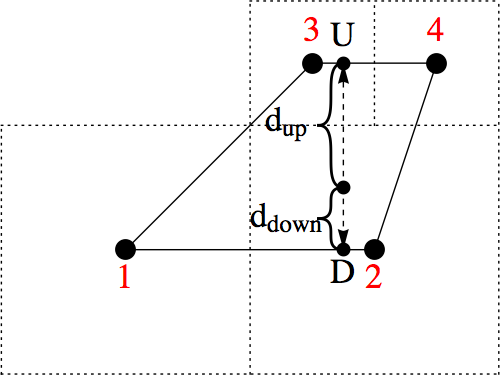
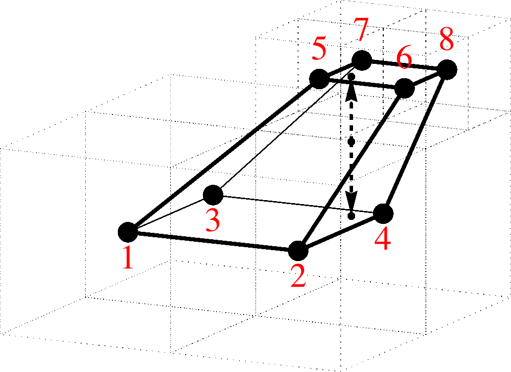
Figure 3: Interpolation on 1-edge for 2D and 3D. Interpolation weights are calculated using distances, $d_{up}$ and $d_{down}$, as: $w_{up}=d_{down}/\left(d_{down}+d_{up}\right)$, $w_{down}=1-w_{up}$, and are applied to the values in endpoints, $U$ and $D$. These values are calculated using linear as on the left and bilinear interpolation (see equation (3)) on the trivial elements as on the right panel, the latter yields weights $w_{i}^{2D}$, $i=1,..,4$, for lower face and $w_{i}^{2D}$, $i=5,..,8$, for upper face, . Then the final interpolation weights are $w_{i}=w^{2D}_{i}w_{down}$, $i=1,..,4$, and $w_{i}=w^{2D}_{i}w_{up}$, $i=5,..,8$. The continuity, for example, at the boundary (1,2,3,4) between this 1-edge and 0-edge (see right panel) is ensured as our interpolation algorithm reduces to bilinear interpolation when point X approaches this boundary, both from below and from above. Also, as the main interpolation line crosses (2-4) edge, the weights of points 1 and 3 become zero, which ensures continuity within resolution 1-edge.

The simplest case is if the central part of the CSB, hence, the whole CSB, is a resolution 1-edge. In this case the interpolation stencil for X, which coincides with its enclosing stencil, consists of Coarser vertices and the Fine $2^{N{-}1}$-cluster, which X projects onto.

The interpolation procedure is a linear interpolation applied to endpoints of the main interpolation line, which are 2 vertices in 1D case or intersection points of the main interpolation line with trivial elements of enclosing stencil in 2D and 3D, the endpoint values are obtained using linear/bilinear interpolation on trivial elements as shown in Figure 3. As mentioned before, we apply this simple algorithm throughout the whole resolution 1-edge. The algorithm quits.

This approach is different from that developed in [17], where the authors decompose corresponding part of a grid into two sorts of shapes in 2D and three sorts of shapes in 3D based on position of the point X within this region. This approach is easy to understand and implement, but our algorithm is simpler and more efficient. We apply the same simple interpolation procedure every time point X falls into a resolution 1-edge independently of its position.

4.2.4 CSB decomposition and interpolation: resolution 2-edge

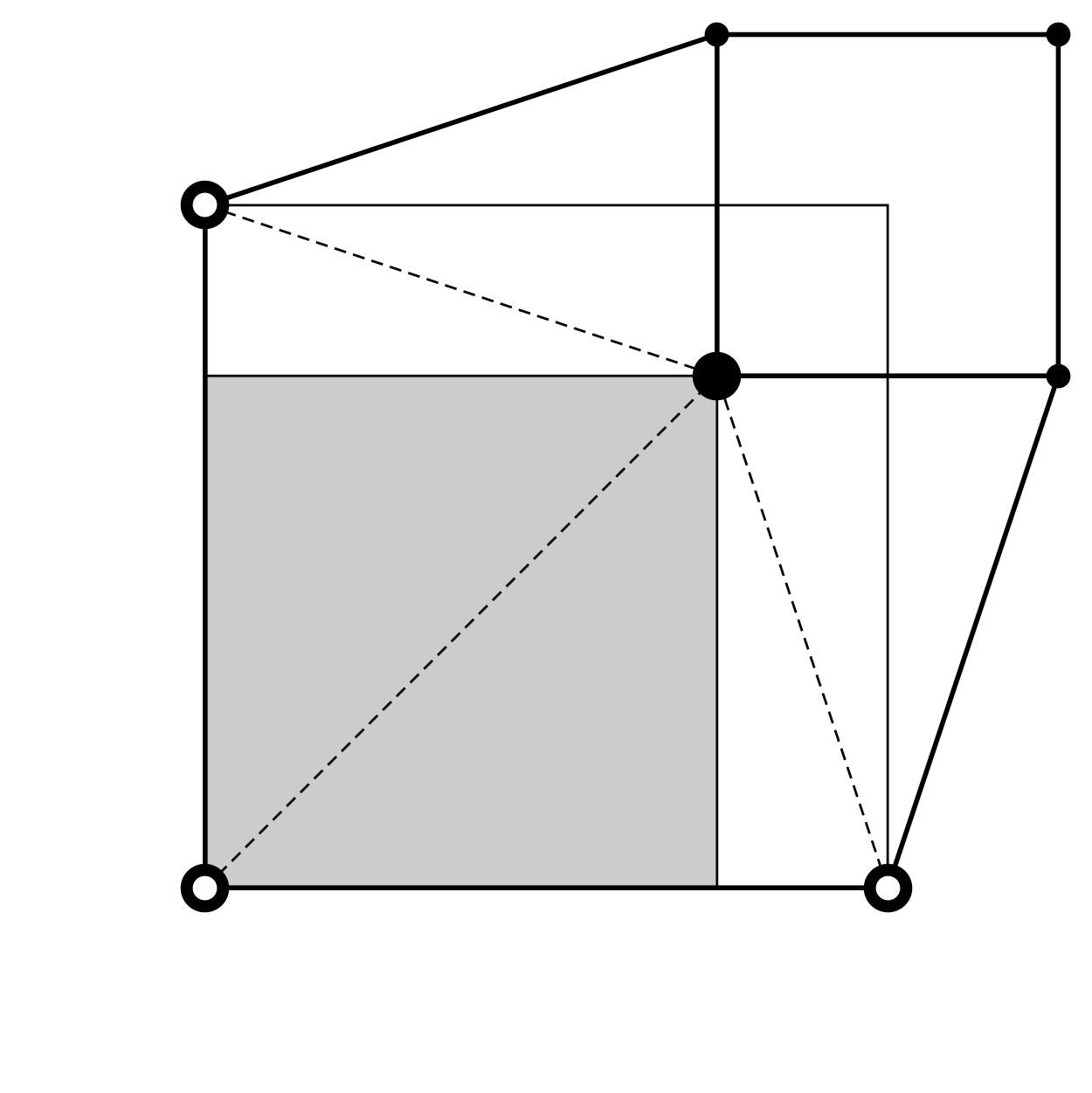
Figure 4: CSB decomposition (top panels only) and interpolation on 2-edge for 2D (top panels) and 3D (bottom panels). Herewith, hollow points are centers of Coarser cells, solid points are those of Finer cells. Here, bolder solid points (panels 4-4) mark Finer vertices of a central quadrangle. Shaded regions show main interpolation planes (which become resolution 2-edges in 2D) for point X (marked for 3D), white regions in top panels are resolution 0- and 1-edges. CSB decomposition is shown with red lines, being dividing lines. Triangulation of the main interpolation plane is shown with dashed lines. It is easy to see from panels 4-4 that interpolation on resolution 2-edges continuously transits to interpolation on resolution 0- and 1-edges through boundaries of main interpolation planes. Note, that certain triangles in the main interpolation plane only partially lay inside a resolution 2-edge with the remaining parts being inside resolution 1-edges.

If the edge type of the central shape derived from level set appears to be 2, then, generally speaking, the CSB decomposes into resolution 1- and 2-edges. Below we provide implementation details for search for the interpolation stencil. Although not difficult for a resolution 2-edge, decomposition of a resolution 3-edge becomes very sophisticated. In order to reduce the computational time spent for the search, we split CSB into rectangular boxes. Based on which particular box the point X falls into, we can eliminate some of the grid points from the extended stencil and reduce the number of simple shapes that may contain point X. We describe this procedure in details for 2-edge and only briefly we outline this for 3-edge in the next section.

Note, that the effective dimensionality in this case is 2. We consider a 2-edge in 2D ($x,y$) space, or a 2-edge in 3D with trivial elements along $z$-axis. Let $x{=}x_{min}$ be the lower face (edge) of the CSB perpendicular to $x$-axis, with $x{=}x_{min}+\Delta x^{(C)}{=}x_{max}$ being its upper face (edge). We divide the CSB by a plane (line), $x{=}x_{min}+\Delta x^{(C)}/4$, if the face $x{=}x_{min}$ intersects at least one Fine cluster. Analogously, we divide the CSB by a plane (line), $x{=}x_{max}-\Delta x^{(C)}/4$, if the face $x{=}x_{max}$ intersects at least one Fine cluster. Repeating the same procedure for $y$-axis, we split CSB into rectangular boxes (see panels 4-4 in Figure 4, splitting is shown in red).

The white rectangular domains in panel 4 in Figure 4 are resolution 1-edges. They are interpolated as described in section 4.2.3 and the algorithm quits.

The shaded boxes form the main interpolation plane for the point X within the resolution 2-edge. It is decomposed into triangles and we apply triangular interpolation. Once we determine, which rectangular box contains X, only a subset of triangles needs to be checked, which makes the algorithm more efficient.

Thus, the interpolation procedure within resolution 2-edge is a triangular interpolation performed on selected vertices in 2D and on selected intersection points of the main interpolation plane with trivial elements in 3D. Again, values in these intersection points are calculated using a linear interpolation on the trivial elements. The product of weights used to calculate these values and those resulting from interpolation procedure in the main interpolation plane yields final interpolation weights. The algorithm quits.

We note that within resolution 2-edges of a 2D grid our algorithm uses the same triangulation as [17], but it is connected to resolution 1-edges differently. We also describe how CSB splitting into rectangular boxes can be used to speed up the search for the interpolation stencil (triangular stencil in this case). Our approach for resolution 2-edges of a 3D grid is different from [17], as the authors use a 3D tessellation, while we use a linear interpolation along the trivial elements and a 2D interpolation on the main interpolation plane, which makes our algorithm simpler.

4.2.5 CSB decomposition and interpolation: resolution 3-edge

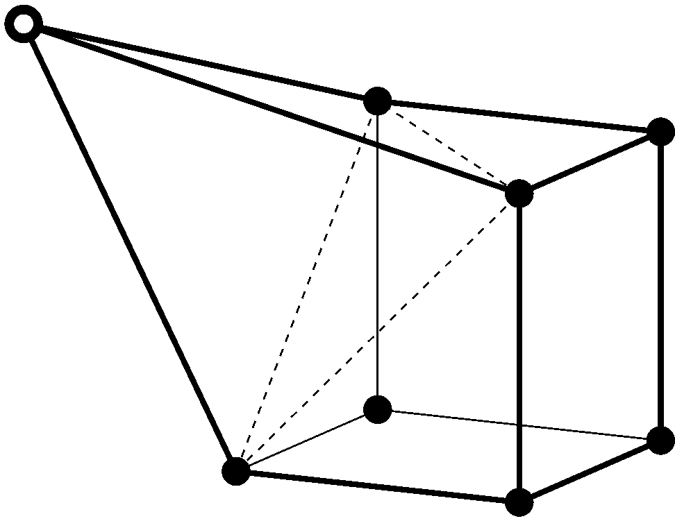
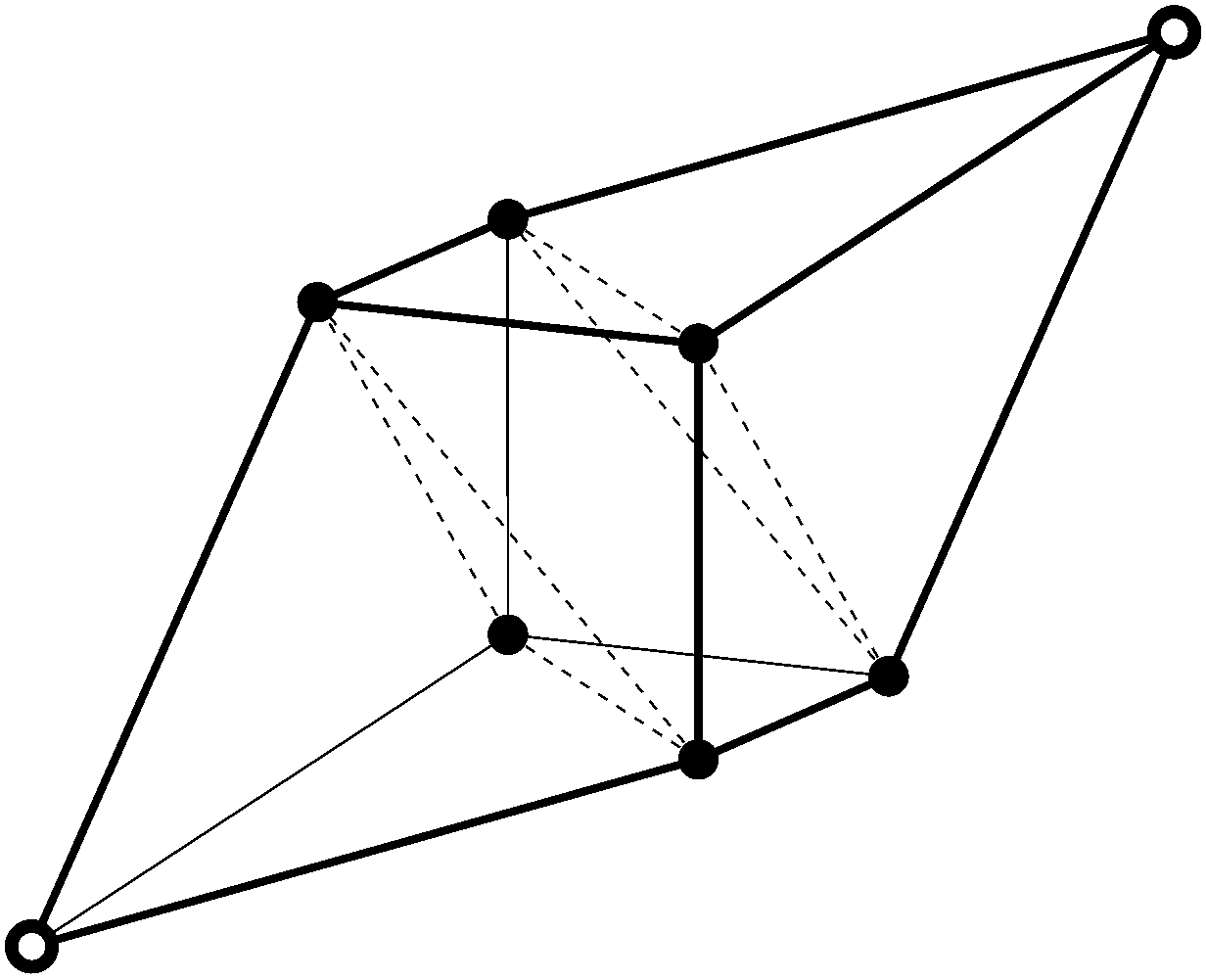
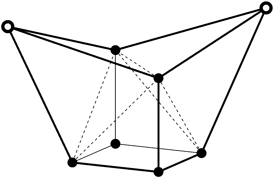
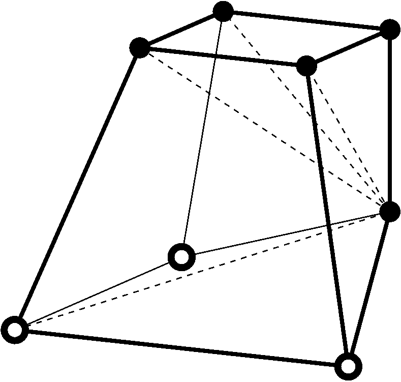
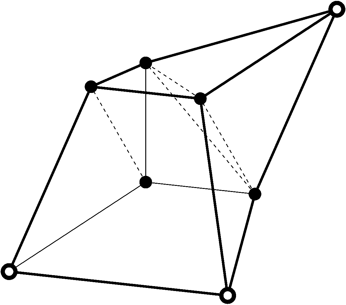
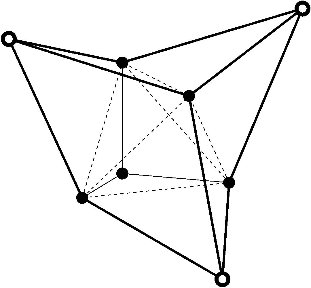
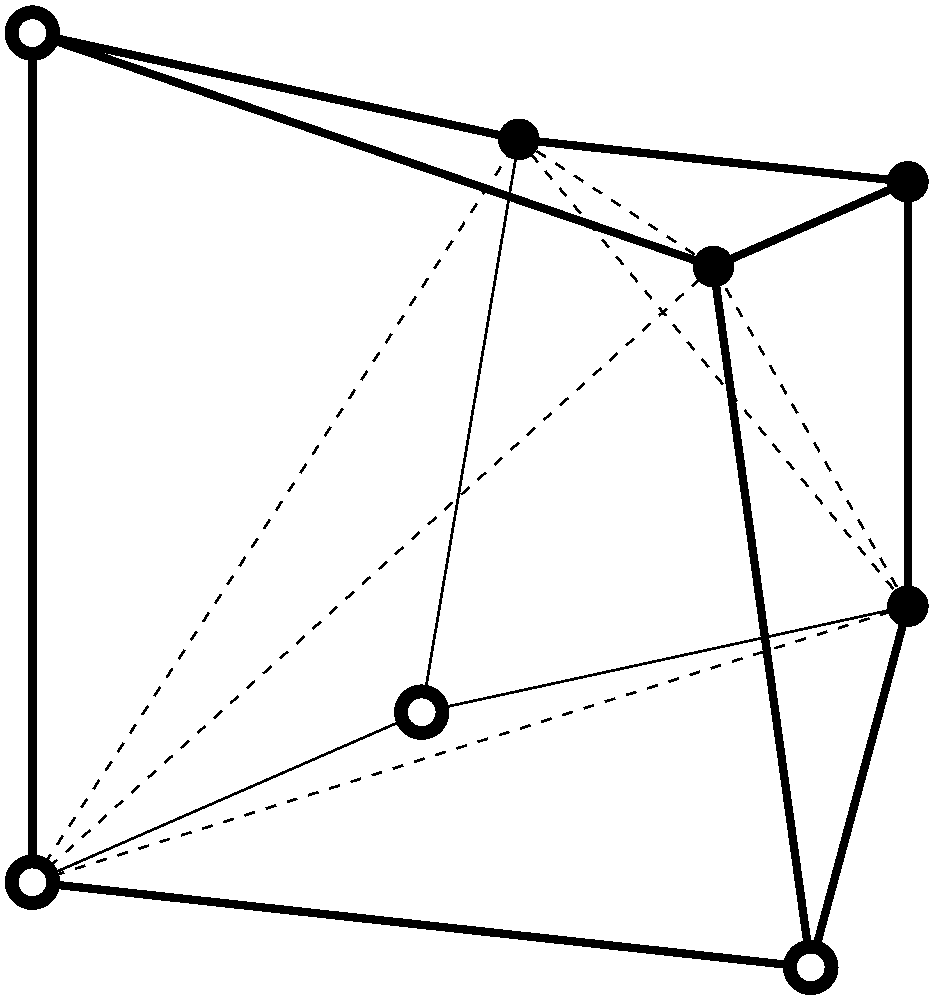
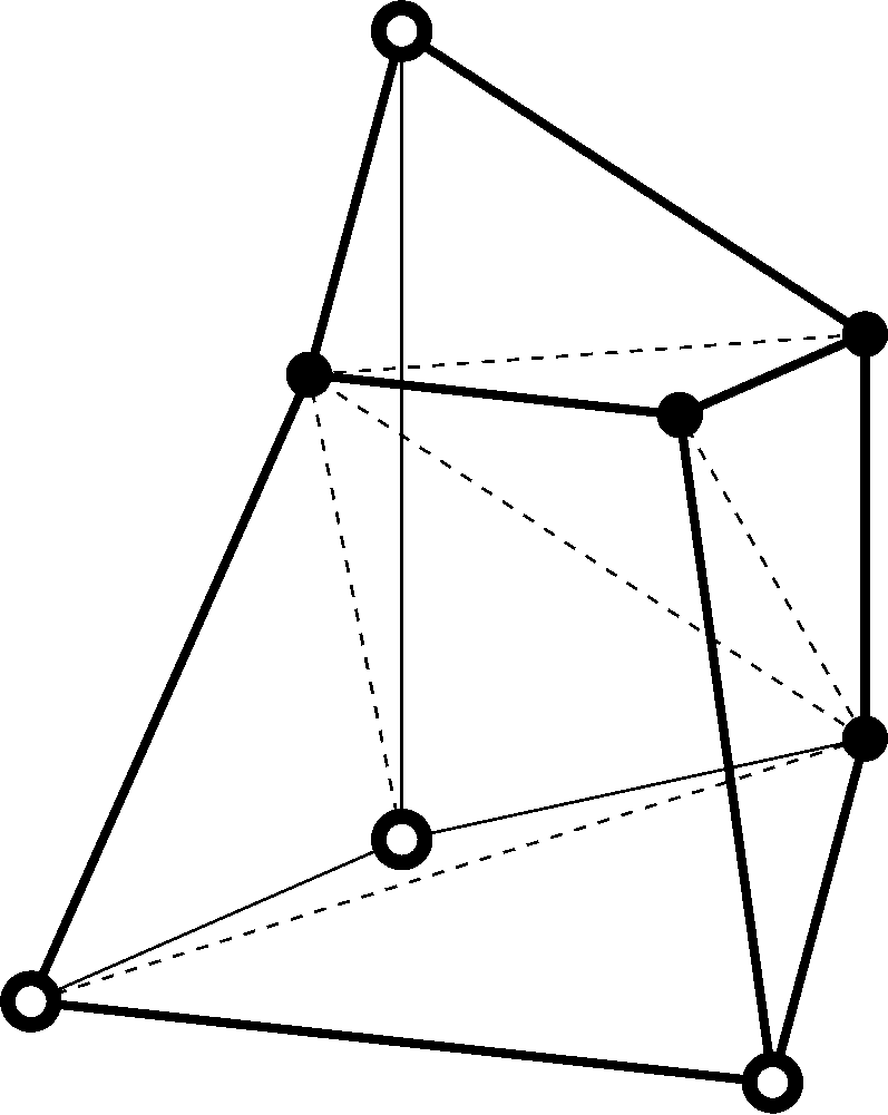
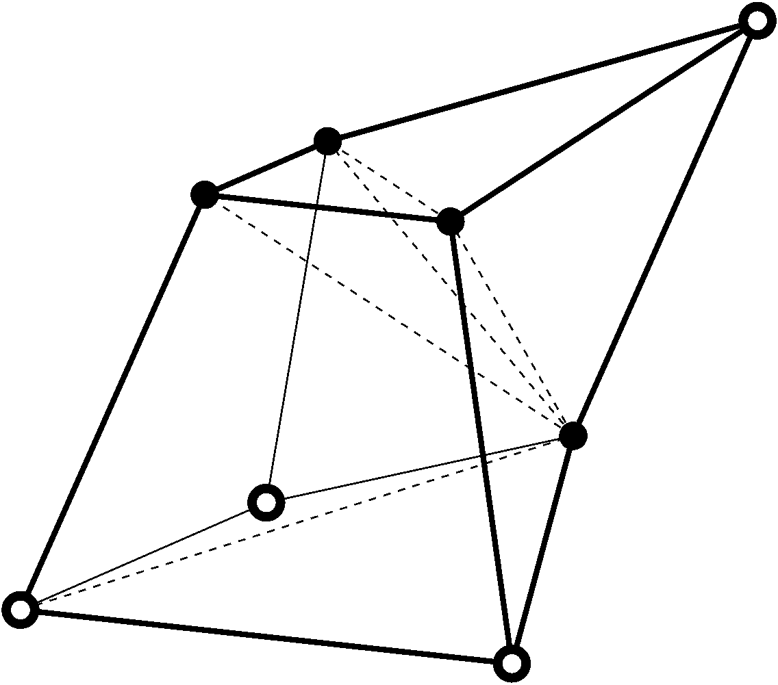
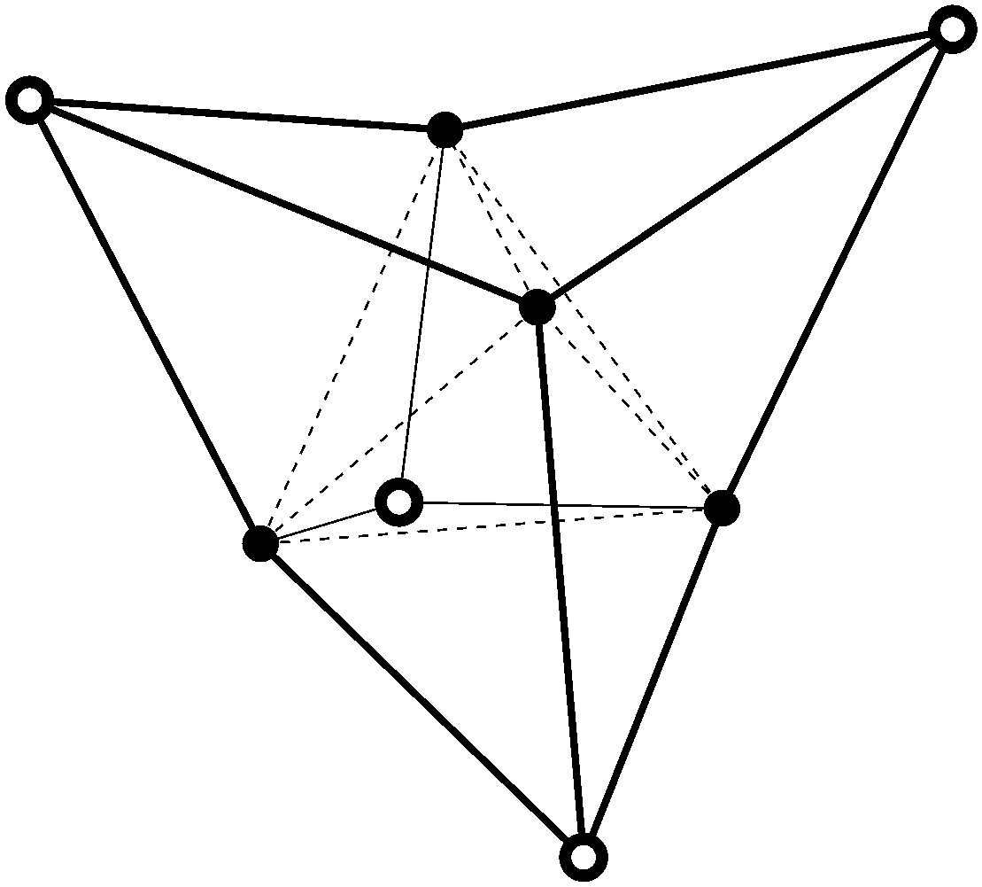
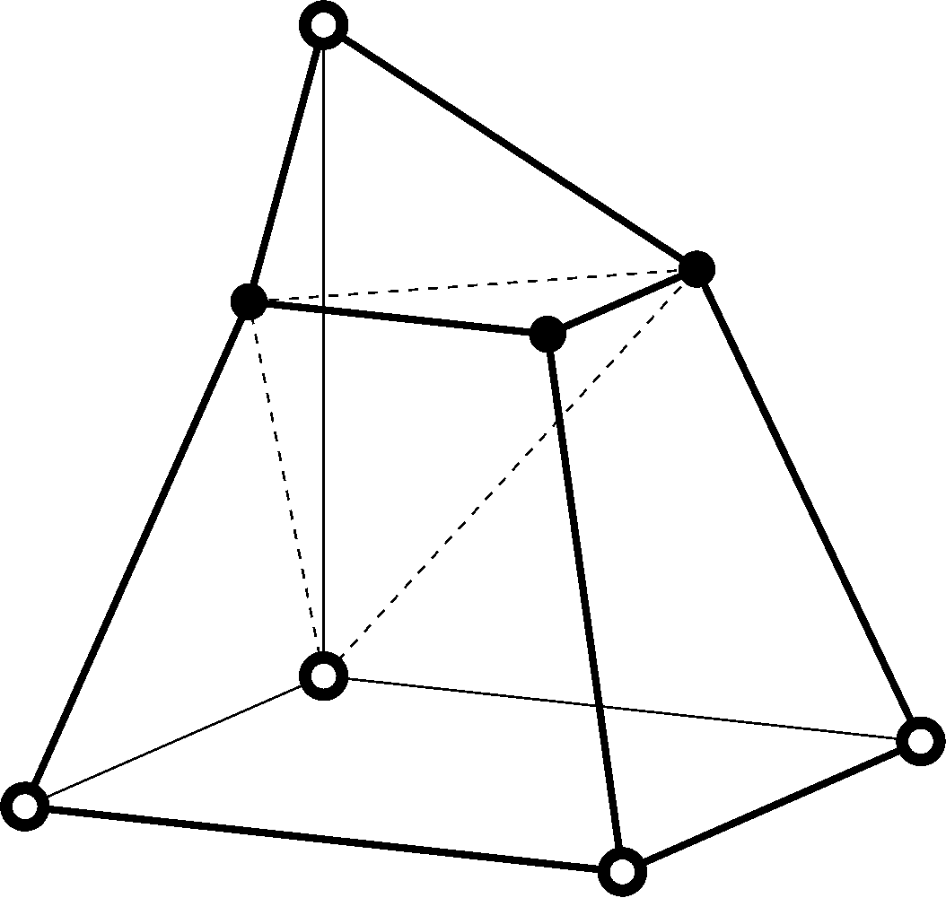
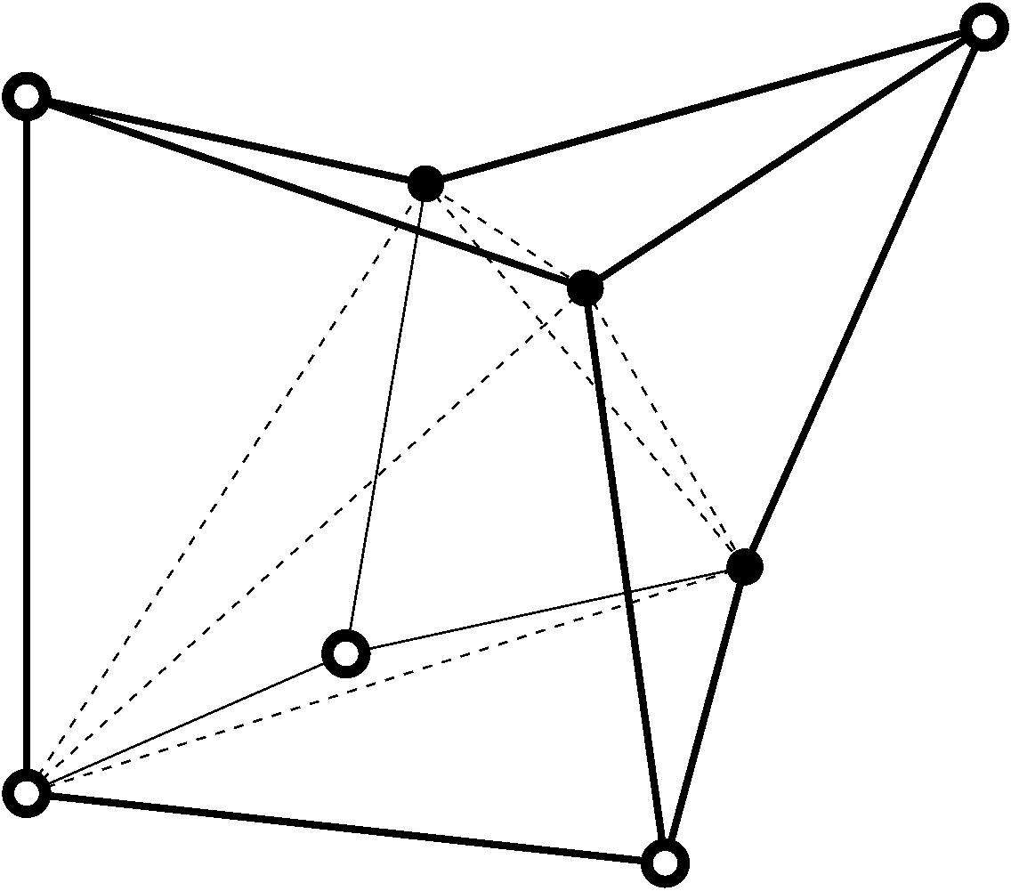
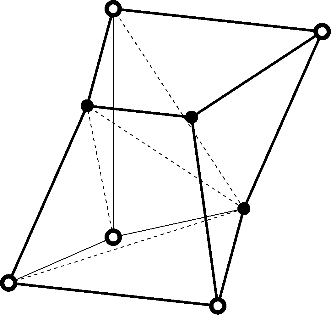
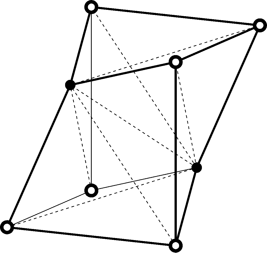
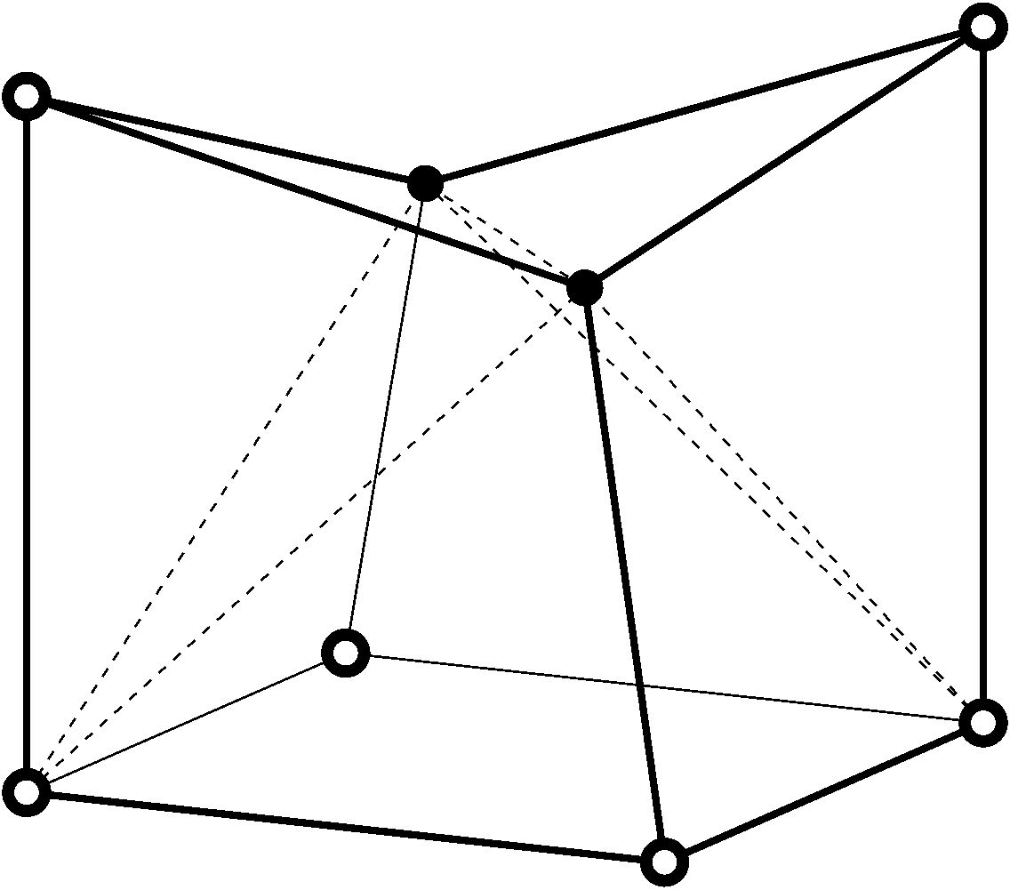
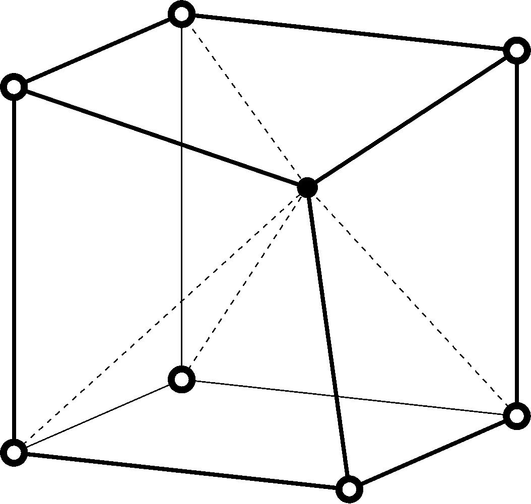
Figure 5: Decomposition of central hexahedra of resolution 3-edges. Particular decomposition for each hexahedron is shown with dashed lines: 5 - tetrahedron and irregular shape; 5 - 2 tetrahedra and irregular shape; 5 - 2 tetrahedra and irregular shape; 5 - rectangular and 2 trapezoidal pyramids; 5 - tetrahedron, rectangular pyramid and wedge; 5 - 5 tetrahedra; 5 - 5 tetrahedra; 5 - 2 tetrahedra and 2 trapezoidal pyramids; 5 - 2 tetrahedra and 2 trapezoidal pyramids; 5 - 5 tetrahedra; 5 - tetrahedron and irregular shape; 5 - 5 tetrahedra; 5 - 2 tetrahedra and 2 trapezoidal pyramids; 5 - 6 tetrahedra; 5 - 2 tetrahedra and irregular shape; 5 - 3 rectangular pyramids.

If the edge type of the central hexahedron appears to be 3, then, generally speaking, the CSB decomposes into resolution 1-, 2- and 3-edges. The approach for interpolation is similar to that applied in the previous section. Now, the dividing planes are introduced in three directions. We sort out domains, which are resolution 1- and 2-edges. Specifically, if one of the CSB faces is fully Coarse, then the rectangular box confined between this face and a Fine 4-cluster is a resolution 1-edge (see panel 6 of Figure 6). Similarly, in configuration presented in panel 6 of Figure 6, with one of the edges of CSB being fully Coarse, several rectangular boxes may be found, which form a domain of the resolution 2-edge with the trivial elements parallel to an isolated Coarse 2-cluster. This can be derived by analyzing the level set and decomposition of the CBS into rectangular boxes. If the point falls into a resolution 1-edge or a resolution 2-edge, the interpolation is performed as described above for such resolution edges in section 4.2.3 and 4.2.4, respectively and the algorithm quits.

If the point X falls into the central box, i.e. the enclosed set of a central shape, then interpolation is performed using the tessellation shown in Figure 5. In this case the interpolation procedure is the same as that in [17]. The algorithm quits.

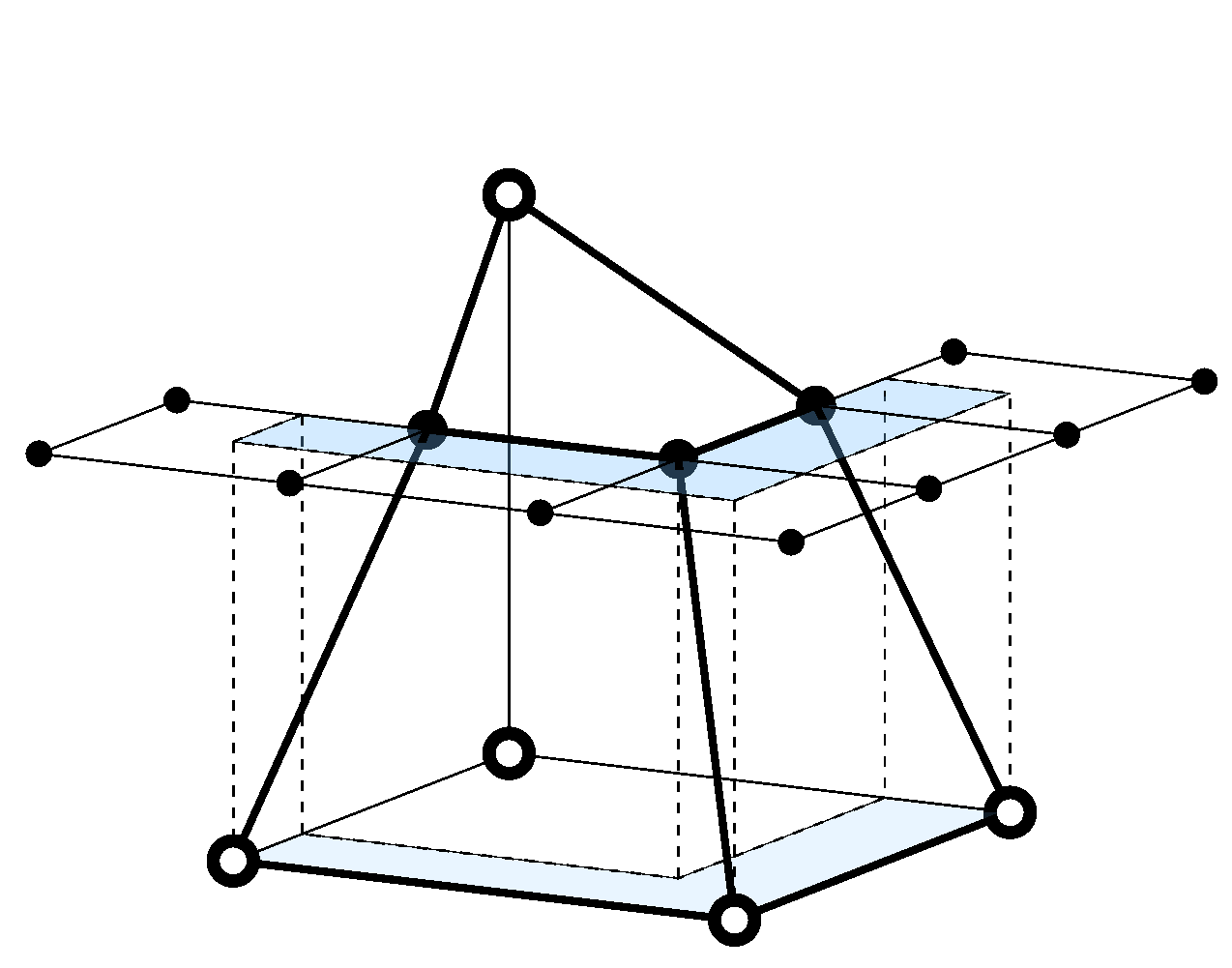
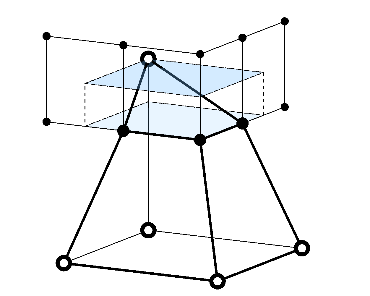
Figure 6: An example of a CSB including resolution 1- and 2-edges. Within the CSB with central octagon 5 in Figure 5 there are domains, which are: 6 - a resolution 1-edge; 6 - a resolution 2-edge. Borders of these domains are shown with dashed lines, their top and bottom faces are shaded.

Finally, for the point X, which doesn’t fall into either the set enclosed by central hexahedron, or resolution 1- and 2-edges, the interpolation stencil is chosen according to resolution 3-edge decomposition outside the central hexahedron into simpler shapes. The interpolation is performed on the resulting shapes. The particular pattern of decomposition is based on the current CSB configuration and the position of the rectangular box X falls into. The idea of the decomposition procedure is given in Figure 7.

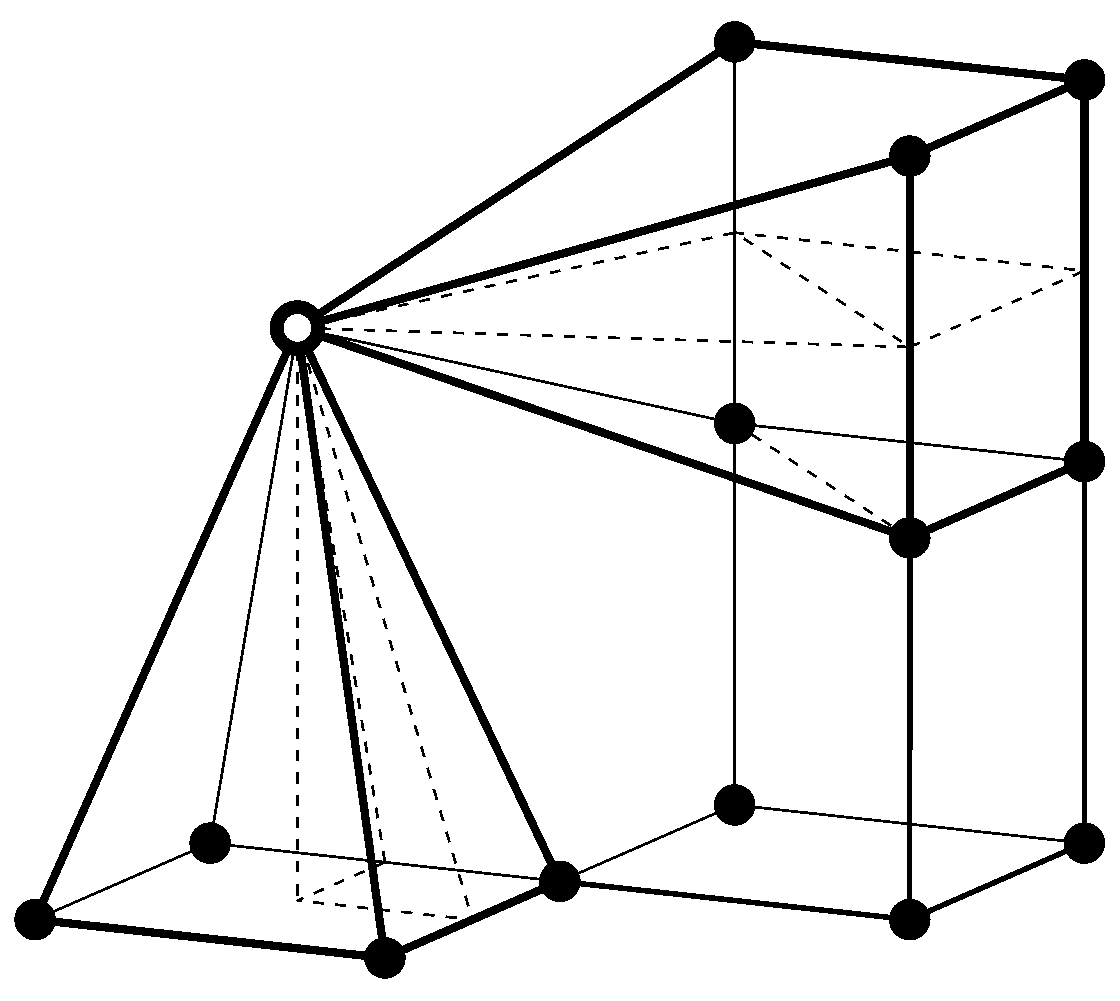
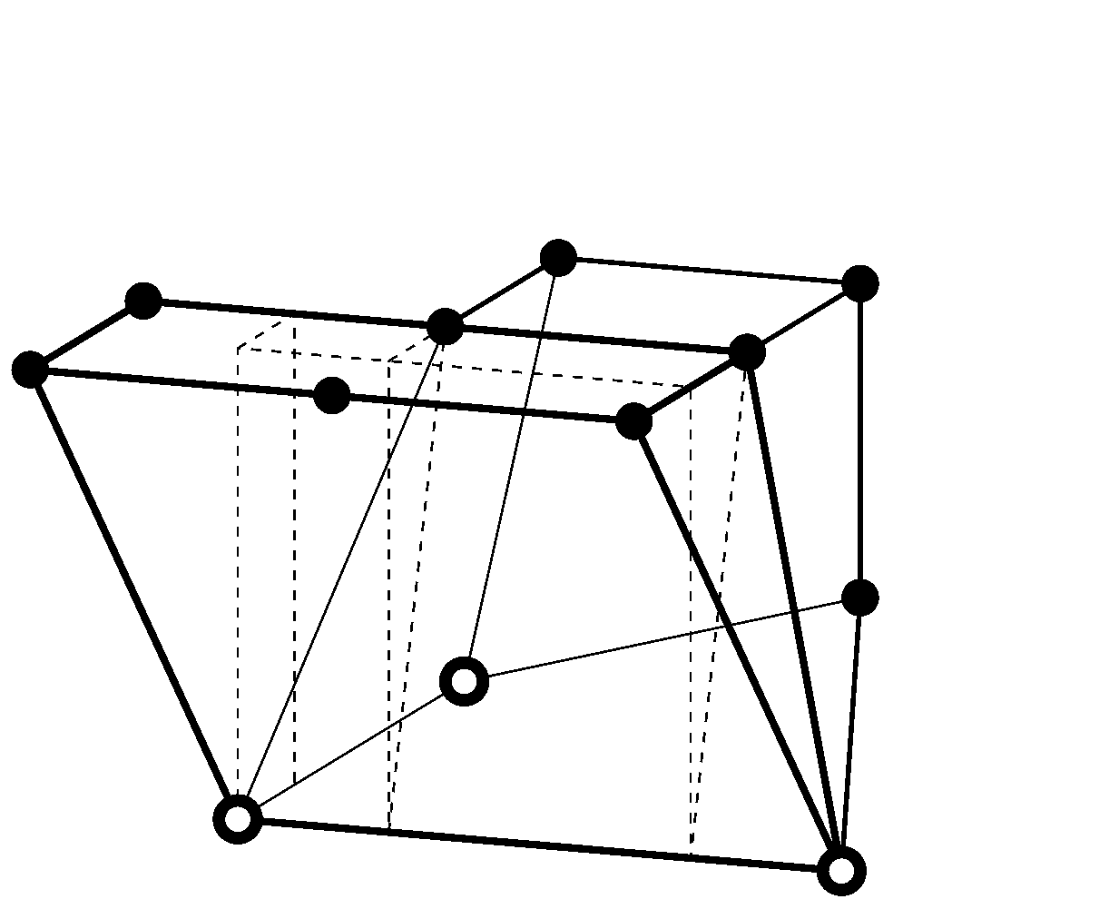
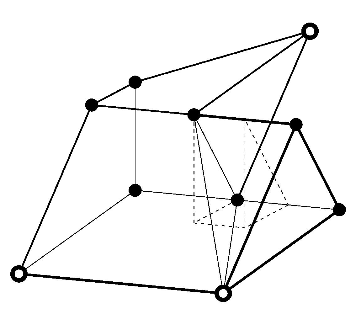
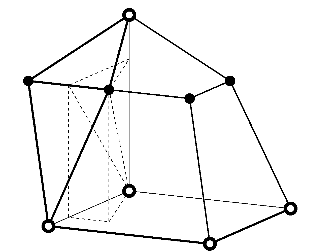
Figure 7: Decomposition of a resolution 3-edge outside of a central hexahedron into simple shapes. Dashed lines show the boundaries of these shapes. Panel 7 shows an isolated Coarse vertex, see panels 5, 5, 5, 5, 5, 5, 5 and 5 in Figure 5, the following shapes may be distinguished: a rectangular pyramid inside the one formed with this Coarse vertex as an apex and either a Fine 4-cluster, or a pair of Fine 2-clusters. The latter may have a triangular prism formed by 6 Fine vertices adjacent to it. Near fully Coarse edges, see panels 5, 5, 5, 5, 5, 5, 5, 5, 5 and 5 in Figure 5, the following shapes may be distinguished: (1) a triangular prism inside a triangular wedge formed by a Coarse edge and either a Fine 4-cluster, or a pair of Fine 2-clusters (panels 7 and 7 respectively); (2) a tetrahedron inside the one formed by a Coarse edge and a Fine 2-cluster (panel 7); (3) an irregular shape inside the one formed by a pair of Coarse edges and a Fine 2-cluster (panel 7). Panel 7 shows a fully Coarse face, see panels 5 and 5 in Figure 5, the following shapes may be distinguished: an irregular shape inside the one formed by a Coarse face and a Fine 2-cluster.

At this point another branch in the CSB decomposition procedure is possible, as long as point X may happen to actually fall into the central hexahedron, rather than into the constructed shape, thus compromising the effort spent for its construction and decomposition. In this case the interpolation is performed on the central hexahedron as described in Figure 5. The advantage of our resolution edge concept is that it allows us to avoid using whenever possible this complicated branch in the algorithm for points falling into resolution 1- and 2-edges.

We emphasize, that at this point our algorithm becomes more complicated than that in [17], though interpolation procedures for points within resolution 3-edge are the same. However, we benefit from the interpolation procedure being simpler on a much larger part of the grid (resolution 1- and 2-edges), which dominate the computational time. Therefore, complication of the algorithm itself and its implementation is merely a trade-off for a higher efficiency.

4.2.6 Interpolation on simple shapes

The interpolation is performed on the shapes a resolution 3-edge decomposes into. In practice, the problem is solved in the following order: for a known decomposition pattern we calculate the interpolation weights for each shape involved, starting with simpler ones. The algorithm quits as soon as all the interpolation weights are positive and less than one, i.e. the point is inside the given shape.

The simplest shape is a tetrahedron, for which there is only one second order accurate interpolation scheme. It is encountered in many possible configurations, certain central hexahedra decompose into a set of tetrahedra (see panels 5, 5, 5, 5 and 5 in Figure 5).

Another simple shape is a triangular wedge prism (see panels 5 in Figure 5 and 7, 7 in Figure 7) or a triangular prism (see panel 7 in Figure 7). Interpolation approach is similar to that for a resolution 2-edge. Triangular interpolation is used in the plane perpendicular to wedge’s side edges, while values in intersection points are obtained using linear interpolation along these edges.

The next shape is a trapezoidal (see panels 5, 5, 5 and 5 in Figure 5) or a rectangular pyramid (see panel 7 in Figure 7). Interpolation is effectively a linear interpolation performed on an apex and projection of a given point along line apex-point onto a base. The value in a projection point is obtained using either bilinear interpolation if a given point projects onto central part of a base, or a triangular interpolation if it projects closer to trapezoid’s legs.

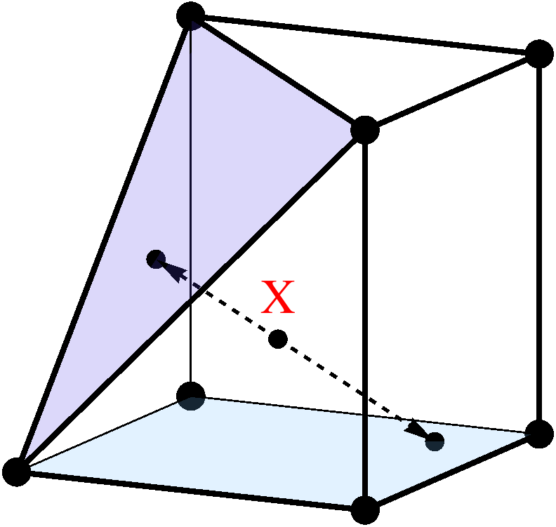
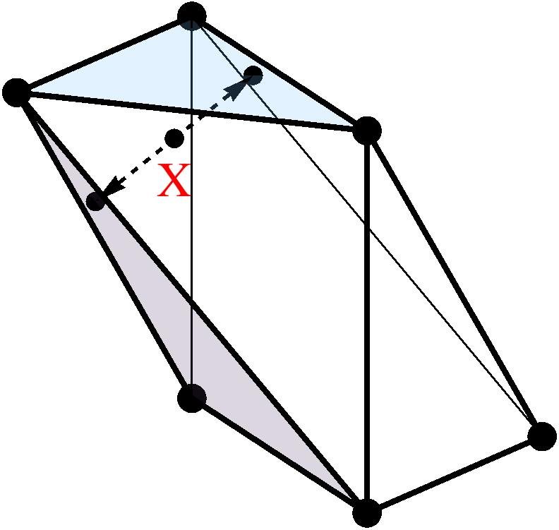
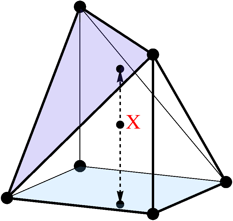
Figure 8: An example of interpolation procedure using a ray tracing. Direction of the ray (dashed line) is chosen to be the longest diagonal of the central hexahedron for the irregular shapes in the tessellations 5, 5 in Figure 5 and a perpendicular to a 4-cluster for all the other irregular shapes (see panels 5 in Figure 5 and 7 and 7 in Figure 7). Shaded faces are those intersected by the ray, interpolation performed on them is either triangular, or bilinear. Linear interpolation is used along the ray to obtain a value in the point X.

For the remaining shapes the approach is the following. The value in a given point X is obtained via linear interpolation on points, resulting from intersection of a ray of a certain direction going through X with faces of a shape. On these faces either triangular, or bilinear interpolation is used. Direction of a ray is chosen to be the longest diagonal of the central hexahedron for the irregular shapes in the tessellations 5 and 5 in Figure 5 and perpendicular to the plane of a 4-cluster for all the other irregular shapes (see irregular shapes 7 and 7 in Figure 7). Examples of such interpolation on irregular shapes is shown in Figure 8.

5 Testing the algorithm

To verify order and continuity of the algorithm the following test is used.

We start from a $2\times 2$ base grid in 2D or a $2\times 2\times 2$ base grid in 3D, i.e. $2^{N}$ grid blocks. Then an arbitrary subset of the $2^{N}$ grid blocks is refined, giving $2^{2^{N}}-1$ possible AMR configurations (15 in 2D and 255 in 3D). The order of accuracy and the continuity are checked for each configuration.

The approximation order is verified as follows. When applied to linear functions of coordinates, the second-order algorithm should reproduce the function exactly, particularly, the coordinates of an arbitrary point on the grid are themselves linear functions ($x(x,y,z)=x$ etc.), therefore, the coordinates of the stencil vertices, once summed up with interpolation weights for arbitrary point X, yield exact coordinates of this point.

Continuity of the algorithm is verified by checking the capability to interpolate a non-linear function of coordinates with no jump in the interpolated values. To each cell a random value in the range $[0.25,0.75]$ in the Finer blocks and in the range $[0,1]$ in the Coarser blocks is assigned. In this way the spatial gradient along direction $i$ of thus sampled function is bounded by the value of $1/\Delta x_{i}^{(C)}$. Two random points are generated, each is displaced in respect to the other by at most $0.01$ along each axis. Then, for a continuous interpolation procedure, the difference between interpolated values is bounded by sufficiently small value. For the set of parameters chosen, this value is $\approx 0.01N$.

The algorithm is tested as a part of nightly tests of SWMF, during each test 20000 random points are generated for both 2D and 3D cases.

6 Conclusion

We have presented a generalization of a bilinear/trilinear interpolation to block-adaptive grids that is continuous and of second order accuracy. The approach employs sequential inheritance of interpolation patterns from lower to higher dimensions, which makes it effective and allows us to avoid excessive logical branching in the implementation of the algorithm. Time performance is comparable to that of a basic bilinear/trilinear interpolation applied to a uniform grid. Thus, the algorithm is well suited to be used for interpolation without degrading the simulation performance. It is applicable to the problems of data visualization as well, such as generation of crack free isosurfaces or extracting smoothly varying data on cut planes and other surfaces.

References

References

- [1] M. J. Berger, P. Colella, Local adaptive mesh refinement for shock hydrodynamics, Journal of Computational Physics 82 (1989) 64–84. doi:10.1016/0021-9991(89)90035-1.
- [2] K. G. Powell, P. L. Roe, T. J. Linde, T. I. Gombosi, D. L. De Zeeuw, A Solution-Adaptive Upwind Scheme for Ideal Magnetohydrodynamics, Journal of Computational Physics 154 (1999) 284–309. doi:10.1006/jcph.1999.6299.
- [3] K. G. Powell, T. I. Gombosi, D. L. De Zeeuw, A. J. Ridley, I. V. Sokolov, Q. F. Stout, G. Tóth, Parallel, Adaptive-Mesh-Refinement MHD for Global Space-Weather Simulations, AIP Conference Proceedings 679 (1) (2003) 807–814. doi:10.1063/1.1618714.
- [4] T. I. Gombosi, K. G. Powell, D. L. D. Zeeuw, C. R. Clauer, K. C. Hansen, W. B. Manchester, A. J. Ridley, I. I. Roussev, I. V. Sokolov, Q. F. Stout, G. Tóth, Solution-Adaptive Magnetohydrodynamics for Space Plasmas: Sun-to-Earth Simulations, Computing in Science and Engg. 6 (2) (2004) 14–35. doi:10.1109/MCISE.2004.1267603.
- [5] K. Powell, D. De Zeeuw, I. Sokolov, G. Tóth, T. Gombosi, Q. Stout, Parallel, AMR MHD for Global Space Weather Simulations, in: T. Plewa, T. Linde, V. Gregory Weirs (Eds.), Adaptive Mesh Refinement - Theory and Applications, Vol. 41 of Lecture Notes in Computational Science and Engineering, Springer Berlin Heidelberg, 2005, pp. 473–490. doi:10.1007/3-540-27039-6-36.
- [6] G. Tóth, I. V. Sokolov, T. I. Gombosi, D. R. Chesney, C. R. Clauer, D. L. de Zeeuw, K. C. Hansen, K. J. Kane, W. B. Manchester, R. C. Oehmke, K. G. Powell, A. J. Ridley, I. I. Roussev, Q. F. Stout, O. Volberg, R. A. Wolf, S. Sazykin, A. Chan, B. Yu, J. Kóta, Space Weather Modeling Framework: A new tool for the space science community, Journal of Geophysical Research (Space Physics) 110 (2005) 12226. doi:10.1029/2005JA011126.
- [7] G. Tóth, D. L. de Zeeuw, T. I. Gombosi, W. B. Manchester, A. J. Ridley, I. V. Sokolov, I. I. Roussev, Sun-to-thermosphere simulation of the 28-30 October 2003 storm with the Space Weather Modeling Framework, Space Weather 5 (2007) 6003. doi:10.1029/2006SW000272.
- [8] G. Tóth, B. van der Holst, I. V. Sokolov, D. L. De Zeeuw, T. I. Gombosi, F. Fang, W. B. Manchester, X. Meng, D. Najib, K. G. Powell, Q. F. Stout, A. Glocer, Y.-J. Ma, M. Opher, Adaptive numerical algorithms in space weather modeling, Journal of Computational Physics 231 (2012) 870–903. doi:10.1016/j.jcp.2011.02.006.
- [9] I. V. Sokolov, I. I. Roussev, T. I. Gombosi, M. A. Lee, J. Kóta, T. G. Forbes, W. B. Manchester, J. I. Sakai, A New Field Line Advection Model for Solar Particle Acceleration, The Astrophysical Journal 616 (2004) L171–L174. doi:10.1086/426812.
- [10] I. V. Sokolov, I. I. Roussev, L. A. Fisk, M. A. Lee, T. I. Gombosi, J. I. Sakai, Diffusive Shock Acceleration Theory Revisited, The Astrophysical Journal 642 (2006) L81–L84. doi:10.1086/504406.
- [11] I. V. Sokolov, I. I. Roussev, MHD turbulence model for global simulations of the solar wind and SEP acceleration, in: G. Li, Q. Hu, O. Verkhoglyadova, G. P. Zank, R. P. Lin, J. Luhmann (Eds.), American Institute of Physics Conference Series, Vol. 1039 of American Institute of Physics Conference Series, 2008, pp. 93–98. doi:10.1063/1.2982491.
- [12] I. V. Sokolov, I. I. Roussev, M. Skender, T. I. Gombosi, A. V. Usmanov, Transport Equation for MHD Turbulence: Application to Particle Acceleration at Interplanetary Shocks, The Astrophysical Journal 696 (2009) 261–267. doi:10.1088/0004-637X/696/1/261.
- [13] P. Colella, J. Bell, N. Keen, T. Ligocki, M. Lijewski, B. van Straalen, Performance and scaling of locally-structured grid methods for partial differential equations, Journal of Physics Conference Series 78 (1) (2007) 012013. doi:10.1088/1742-6596/78/1/012013.
- [14] S. N. Borovikov, I. A. Kryukov, I. E. Ivanov, Method of Tetrahedral Mesh Generation for Regions with Curvilinear Boundaries, Astronomical Society of the Pacific Conference Series 359 (2006) 295–301.
- [15] P. MacNeice, K. M. Olson, C. Mobarry, R. de Fainchtein, C. Packer, PARAMESH: A parallel adaptive mesh refinement community toolkit, Computer Physics Communications 126 (2000) 330–354. doi:10.1016/S0010-4655(99)00501-9.
- [16] I. V. Sokolov, K. G. Powell, T. I. Gombosi, I. I. Roussev, A TVD principle and conservative TVD schemes for adaptive Cartesian grids, Journal of Computational Physics 220 (2006) 1–5. doi:10.1016/j.jcp.2006.07.021.
- [17] G. Weber, O. Kreylos, T. J. Ligocki, J. M. Shalf, H. Hagen, B. Hamann, K. I. Joy, Extraction of crack-free isosurfaces for adaptive mesh refinement data, in: D. S. Ebert, J. M. Favre, R. Peikert (Eds.), Data Visualization 2001 - Proceedings of Joint Eurographics/IEEE TCVG Symposium on Visualization, Eurographics Association, IEEE, Springer Verlag, 2001, pp. 25–34.
- [18] G. H. Weber, O. Kreylos, T. J. Ligocki, J. M. Shalf, H. Hagen, B. Hamann, K. I. Joy, K. liu Ma, High-quality volume rendering of adaptive mesh refinement data, in: In Proceedings of Vision, Modeling, and Visualization 2001, Press, 2001, pp. 121–128.
- [19] P. J. Moran, D. Ellsworth, Visualization of AMR Data With Multi-Level Dual-Mesh Interpolation., IEEE Trans. Vis. Comput. Graph. 17 (12) (2011) 1862–1871.