ON THE CAUSE OF SOLAR-LIKE EQUATORWARD MIGRATION IN GLOBAL
CONVECTIVE DYNAMO SIMULATIONS

Abstract

We present results from four convectively-driven stellar dynamo simulations in spherical wedge geometry. All of these simulations produce cyclic and migrating mean magnetic fields. Through detailed comparisons, we show that the migration direction can be explained by an $\alpha\Omega$ dynamo wave following the Parker–Yoshimura rule. We conclude that the equatorward migration in this and previous work is due to a positive (negative) $\alpha$ effect in the northern (southern) hemisphere and a negative radial gradient of $\Omega$ outside the inner tangent cylinder of these models. This idea is supported by a strong correlation between negative radial shear and toroidal field strength in the region of equatorward propagation.

1. Introduction

Just over 50 yr after the paper by Maunder (1904), in which he showed for the first time the equatorward migration (EM) of sunspot activity in a time–latitude (or butterfly) diagram, Parker (1955) proposed a possible solution: migration of an $\alpha\Omega$ dynamo wave along lines of constant angular velocity $\Omega$ (Yoshimura, 1975). Here, $\alpha$ is related to kinetic helicity and is positive (negative) in the northern (southern) hemisphere (Steenbeck et al., 1966). To explain EM, $\mbox{\boldmath$\nabla$}{}\Omega$ must point in the negative radial direction. However, application to the Sun became problematic with the advent of helioseismology showing that $\nabla_{\!r}\Omega$ is actually positive at low latitudes where sunspots occur (Schou et al., 1998), implying poleward migration (PM). This ignores the near-surface shear layer where a negative $\nabla_{\!r}\Omega$ (Thompson et al., 1996) could cause EM (Brandenburg, 2005). An alternative solution was offered by Choudhuri et al. (1995), who found that in $\alpha\Omega$ dynamo models with spatially separated induction layers the direction of migration can also be controlled by the direction of meridional circulation at the bottom of the convection zone, where the observed poleward flow at the surface must lead to an equatorward return flow. Finally, even with just uniform rotation, i.e., in an $\alpha^{2}$ dynamo as opposed to the aforementioned $\alpha\Omega$ dynamos, it may be possible to obtain EM due to the fact that $\alpha$ changes sign at the equator (Baryshnikova & Shukurov, 1987; Rädler & Bräuer, 1987; Mitra et al., 2010; Warnecke et al., 2011).

Meanwhile, global dynamo simulations driven by rotating convection in spherical shells have demonstrated not only the production of large-scale magnetic fields, but, in some cases, also EM (Käpylä et al., 2012, 2013; Warnecke et al., 2013b; Augustson et al., 2013). Although this seemed to be successful in reproducing Maunder’s observation of EM, the reason remained unclear. Noting the agreement between their simulation and the $\alpha^{2}$ dynamo of Mitra et al. (2010) in terms of the $\pi/2$ phase shift between poloidal and toroidal fields near the surface, as well as their similar amplitudes, Käpylä et al. (2013) suggested such an $\alpha^{2}$ dynamo as a possible underlying mechanism. Yet another possibility is that $\alpha$ can change sign if the second term in the estimate for $\alpha$ (Pouquet et al., 1976),

$$\alpha={\tau_{\rm c}\over 3}\left(-\overline{\mbox{\boldmath$\omega$}{}\cdot\mbox{\boldmath$u$}{}}+{\overline{\mbox{\boldmath$j$}{}\cdot\mbox{\boldmath$b$}{}}\over\overline{\rho}}\right),$$ (1)

becomes dominant near the surface, where the mean density $\overline{\rho}$ becomes small. Here, $\mbox{\boldmath$\omega$}{}=\mbox{\boldmath$\nabla$}{}\times\mbox{\boldmath$u$}{}$ is the vorticity, $u$ is the small-scale velocity, $\mbox{\boldmath$j$}{}=\mbox{\boldmath$\nabla$}{}\times\mbox{\boldmath$b$}{}/\mu_{0}$ is the current density, $b$ is the small-scale magnetic field, $\mu_{0}$ is the vacuum permeability, $\tau_{\rm c}$ is the correlation time of the turbulence, and overbars denote suitable (e.g., longitudinal) averaging. However, an earlier examination by Warnecke et al. (2013a) showed that the data do not support this idea, i.e., the contribution from the second term is not large enough. Furthermore, the theoretical justification for Equation (1) is questionable (Brandenburg et al., 2008).

A potentially important difference between the models of Käpylä et al. (2012, 2013) and those of other groups (Ghizaru et al., 2010; Racine et al., 2011; Brown et al., 2011; Augustson et al., 2012, 2013; Nelson et al., 2013) is the use of a blackbody condition for the entropy and a radial magnetic field on the outer boundary. The latter may be more realistic for the solar surface (Cameron et al., 2012).

It should be noted that a near-surface negative shear layer similar to the Sun was either not resolved in the simulations of Käpylä et al. (2012, 2013), or, in the case of Warnecke et al. (2013b), such a layer did not coincide with the location of EM. Instead, most of these simulations show a strong tendency for the contours of angular velocity to be constant on cylinders. Some of them even show a local minimum of angular velocity at mid-latitudes. Indeed, Augustson et al. (2013) identified EM with the location of the greatest latitudinal shear at a given point in the cycle and find that also weak negative radial shear plays a role. latitudinal shear at a given point in the cycle and find that also weak negative radial shear plays a role.

In this Letter, we show through detailed comparison among four models that it is this local minimum, where $\nabla_{\!r}\Omega<0$ and $\alpha>0$, which explains the EM as a Parker dynamo wave traveling equatorward. While we do not expect this to apply to Maunder’s observed EM in the Sun, it does clarify the outstanding question regarding the origin of EM in the simulations. A clear understanding of these numerical experiments is a prerequisite for a better understanding of the processes causing EM in the Sun.

2. Strategy

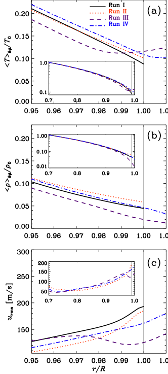
Figure 1.— Radial profiles of azimuthally and latitudinally averaged temperature $\langle T\rangle_{\theta\phi}$ (a), density $\langle\rho\rangle_{\theta\phi}$ (b), and rms velocity $u_{\rm rms}$ (c) near the surface, normalized by their values at the bottom of the domain $T_{0}$, $\rho_{0}$, or in m/s respectively. The inlays show the entire radial extent. The solid black lines indicate Run I, red dotted Run II, purple dashed Run III, and blue dash-dotted Run IV. The thin black lines represent the surface ($r=R$).

To isolate effects arising from changes in the $\alpha$ effect and the differential rotation, we consider four models. Our reference model, Run I, is the same model presented in Käpylä et al. (2012) as their Run B4m and in as Käpylä et al. (2013) their Run C1. Run II is a run in which the subgrid scale (SGS) Prandtl number, $\mbox{\rm Pr}_{\rm SGS}=\nu/\overline{\chi}_{\rm SGS}$, is reduced from 2.5 to 0.5, and the magnetic Prandtl number, $\mbox{\rm Pr}_{M}=\nu/\eta$, is reduced from 1 to 0.5. Here $\nu$ is the viscosity, $\eta$ is the magnetic diffusivity, and $\overline{\chi}_{\rm SGS}$ is the mean SGS heat diffusivity. We keep $\nu$ fixed so the effect of lowering $\mbox{\rm Pr}_{\rm SGS}$ is that the SGS diffusion is more efficiently smoothing out entropy variations. For stars, the relevant value of $\mbox{\rm Pr}_{\rm SGS}$ is well below unity, but such cases are difficult to simulate numerically. In Runs III and IV, we have replaced the outer radiative boundary condition by a cooling layer (see Warnecke et al., 2013b, for the implementation and the profile) above fractional radii $r/R=0.985$ and $1.0$, respectively; see Figure 1(a) and (b) for the radial temperature and density profiles. Here, $R$ is the solar radius. The cooling profile of Run III leads to a stronger density decrease and suppression of $u_{\rm rms}$ than in the other runs; see Figure 1(b) and (c). Besides the differences in the fluid and magnetic Prandtl numbers (Run II) and in the upper thermal boundary condition (Runs III and IV), the setups are equal. We can therefore isolate the origin of the difference in the migration pattern of the toroidal field.

Our simulations are done in a wedge $|90^{\circ}-\theta|\leq 75^{\circ}$, $0<\phi<90^{\circ}$, and $R-\Delta R\leq r\leq R+\delta R_{C}$, where $\theta$ is colatitude, $\phi$ is longitude, $r$ is radius, $\Delta R=0.3\,R$ and $\delta R_{C}=0.01\,R$ is the extension by the cooling layer in Runs III and IV. We solve the equations of compressible magnetohydrodynamics using the Pencil Code. The basic setup of these four models is identical to previous work; the details can be found in Käpylä et al. (2013) and Warnecke et al. (2013b). We scale our results to physical units following Käpylä et al. (2013, 2014) and choose a rotation rate of $\Omega_{0}=5\Omega_{\sun}$, where $\Omega_{\sun}=2.7\times 10^{-6}\,{\rm s}$ is the solar value.

3. Results

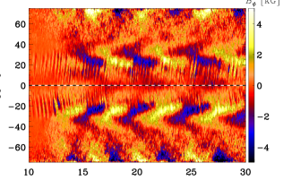
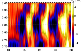
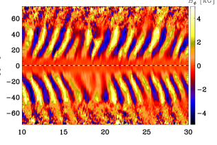
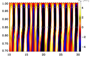
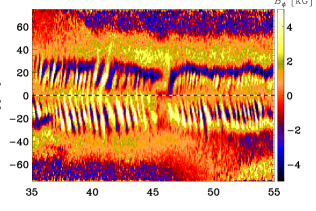
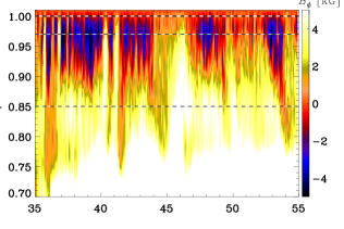
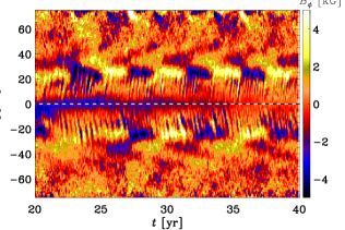
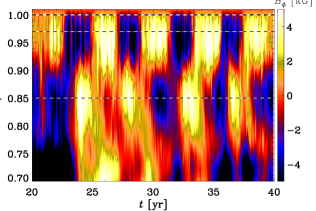
Figure 2.— Time evolution of the mean toroidal magnetic field $\overline{B}_{\phi}$ in the convection zone for Runs I, II, III, and IV, from top to bottom. In the left column, the radial cut is shown at $r=0.98\,R$, and, in the right column, the latitudinal cut at $90-\theta=25^{\circ}$. The dashed horizontal lines show the location of the equator at $\theta=\pi/2$ (left) and the radii $r=R$, $r=0.98\,R$ and $r=0.85\,R$ (right).

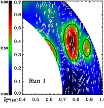
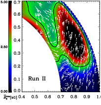
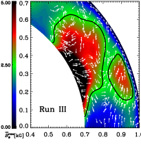
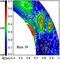
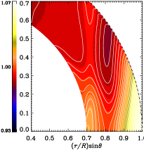
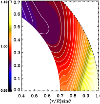
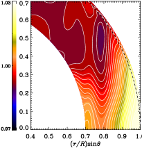
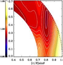
Figure 3.— Top row: color coded $\overline{B}_{\phi}^{\rm rms}$ during the saturated stage for Runs I–IV (left to right). White arrows show the direction of migration $\mbox{\boldmath$\xi$}{}_{\rm mig}(r,\theta)=-\alpha\hat{\mbox{\boldmath$e$}}{}_{\phi}\times\mbox{\boldmath$\nabla$}{}\Omega$; see Equation (3). The black solid lines indicate isocontours of $\overline{B}_{\phi}$ at 2.5 kG. Bottom row: $\Omega(r,\theta)/\Omega_{0}$ for the same runs. The dashed lines indicate the surface ($r=R$).

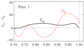
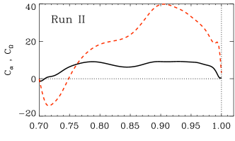
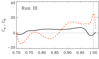
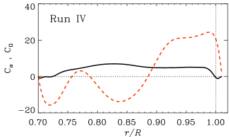
Figure 4.— Local dynamo parameters $C_{\alpha}$ and $C_{\Omega}$ for Runs I–IV. $C_{\alpha}$ (solid black line) and $C_{\Omega}$ (dashed red line) for 25^∘ latitude in the northern hemisphere as a function of $r$.

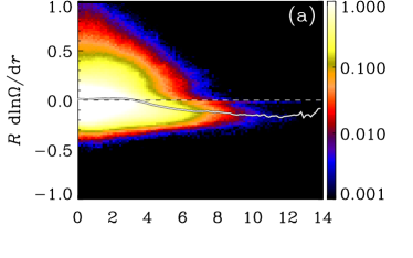
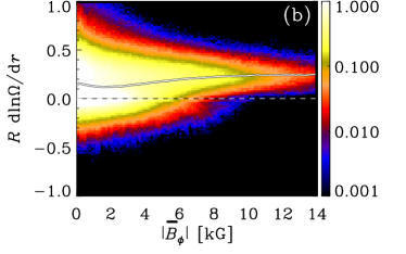
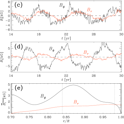
Figure 5.— Panels (a) and (b): correlation of $|\overline{B}_{\phi}|$ from the latitudinal band $\pm 15^{\circ}-\pm 40^{\circ}$ and the logarithmic gradient of $\Omega$ for Runs I (a) and II (b). Overplotted are the mean (white) and the zero lines (white-black dashed). (c) and (d): phase relation between $\overline{B}_{\phi}$ (black) and $\overline{B}_{r}$ (red) at 25^∘ latitude and $r=0.98\,R$ (c) and at $r=0.84\,R$ (d) for Run I. (e): Time-averaged radial dependence of $\overline{B}_{\phi}^{\rm rms}$ (black) and $\overline{B}_{r}^{\rm rms}$ (red) at 25^∘ latitude for Run I.

We begin by comparing the evolution of the mean toroidal field $\overline{B}_{\phi}$ using time–latitude and time–depth diagrams; see Figure 2. In Run I, $\overline{B}_{\phi}$ migrates equatorward between $\pm$10^∘ and $\pm$40^∘ latitude, and becomes strongly concentrated around $r=0.8-0.9\,R$. The cycle period is around five years. In Run IV, the evolution of $\overline{B}_{\phi}$ is similar to Run I. Therefore, the blackbody boundary condition is not a necessity for EM. In both runs, a poleward migrating high-frequency dynamo wave is superimposed on the EM, as already seen in Käpylä et al. (2012, 2013). By contrast, in Run II, $\overline{B}_{\phi}$ migrates poleward between $\pm$10^∘ and $\pm$45^∘ latitude. The field is strongest at $r=0.85-0.98\,R$ and the cycle period is about 1.5 yr. This is clearly shorter than the cycle in Runs I and IV, but significantly longer than the superimposed poleward dynamo wave in those runs. In Run III, $\overline{B}_{\phi}$ has two superimposed field patterns: one with PM similar in frequency and location to that of Runs I and IV, and a quasi-stationary pattern with unchanged field polarity for roughly 20 yr. The poleward migrating field appears in the upper 10% of the convection zone, whereas the non-migrating field is dominant in the lower half of the convection zone.

The distribution of $\overline{B}_{\phi}$ in the meridional plane can be seen in the top row of Figure 3, where we plot the rms of the mean toroidal magnetic field, time-averaged over the saturated stage, $\overline{B}_{\phi}^{\rm rms}\equiv\langle\overline{B}_{\phi}^{2}\rangle^{1/2}_{t}$. In Run I, it reaches 4 kG and is concentrated at mid-latitudes and mid-depths. The field structures are aligned with the rotation axis. Additionally, there is a slightly weaker ($\approx$3 kG) field concentration closer to the equator and surface. A similar field pattern can be found in Run IV, but the field concentrations are somewhat weaker. In Run II, $\overline{B}_{\phi}^{\rm rms}$ is concentrated closer to the surface with a larger latitudinal extent than in Run I. The shape of the field structure is predominantly aligned with the latitudinal direction. In Run III, there is some near-surface field enhancement similar to Run I, but closer to the equator. However, the maximum of $\overline{B}_{\phi}^{\rm rms}$ is near the bottom of the convection zone, although at higher latitudes it occupies nearly the entire convection zone.

Next, we compare the differential rotation profiles of the runs; see the bottom row of Figure 3. All runs develop cylindrical contours of constant rotation as a dominant pattern. However, Runs I, III, and IV possess a local minimum of angular velocity, implying the existence of a negative $\nabla_{\!r}\Omega$, between $\pm$15^∘ and $\pm$40^∘ latitude, which is the same latitude range where EM was found in Runs I and IV. In Run II, the contours of constant angular velocity are nearly cylindrical, but with a slight radial inclination, which is more than in Run I. This is expected due to the enhanced diffusive heat transport and is also seen in other global simulations (e.g. Brun & Toomre, 2002; Brown et al., 2008), where $\mbox{\rm Pr}_{\rm SGS}$ is closer to or below unity. Unlike in Runs I, III, and IV, there is no local minimum of $\Omega$. This can be attributed to the higher value of the SGS heat diffusivity in Run II, which smoothes out entropy variations, leading to a smoother rotation profile via the baroclinic term in the thermal wind balance (see corresponding plots and discussion in Warnecke et al., 2013b).

Furthermore, we calculate the local dynamo numbers

$$C_{\alpha}={\alpha\,\Delta R\over\eta_{\rm t0}},\quad C_{\Omega}={\nabla_{\!r}\Omega\,\Delta R^{3}\over\eta_{\rm t0}},$$ (2)

where $\eta_{\rm t0}=\alpha_{\rm MLT}H_{p}u_{\rm rms}(r,\theta)/3$ is the estimated turbulent diffusivity with the mixing length parameter $\alpha_{\rm MLT}=5/3$, the pressure scale height $H_{p}$, the turbulent rms velocity $u_{\rm rms}(r,\theta)$, and $\alpha(r,\theta)$ is estimated using Equation (1); see also Käpylä et al. (2013). In Figure 4 we plot $C_{\alpha}$ and $C_{\Omega}$ as functions of radius for 25^∘ latitude for Runs I–IV. The $C_{\alpha}$ profiles in all the runs are similar: the quantity is almost always positive, except for a narrow and weak dip to negative values at the very bottom of the simulation domain. The only two exceptions are Runs III and IV, where the cooling layer causes $C_{\alpha}$ to decrease already below (Run III) or just above (Run IV) the surface, becoming even weakly negative there. The reason is a sign change of the kinetic helicity caused by the sign change of entropy gradient. The $C_{\Omega}$ profiles are similar for Runs I, III, and IV. There are two regions of negative values in the lower and middle part of the convection zone, with positive values near the surface. In the middle of the convection zone, these profiles coincide with clearly positive values of $C_{\alpha}$, as required for EM. For Run II, the profiles of $C_{\Omega}$ are markedly different: despite the negative dip at the bottom of the convection zone, the values of $C_{\Omega}$ are generally positive and larger in magnitude than for Runs I, III, and IV. This suggests PM throughout most of the convection zone.

To investigate this in more detail, we calculate the migration direction $\mbox{\boldmath$\xi$}{}_{\rm mig}$ as (Yoshimura, 1975)

$$\mbox{\boldmath$\xi$}{}_{\rm mig}(r,\theta)=-\alpha\hat{\mbox{\boldmath$e$}}{}_{\phi}\times\mbox{\boldmath$\nabla$}{}\Omega,$$ (3)

where $\hat{\mbox{\boldmath$e$}}{}_{\phi}$ is the unit vector in the $\phi$-direction. Note that this and our estimated $\alpha(r,\theta)$ using Equation (1) is a strong simplification of the, in general, tensorial properties. In all of our runs, $\alpha$ is on average positive (negative) in the northern (southern) hemisphere.

The migration direction $\mbox{\boldmath$\xi$}{}_{\rm mig}$ is plotted in the top row of Figure 3 for the northern hemispheres of Runs I–IV. The white arrows show the calculated normalized migration direction on top of the color coded $\overline{B}_{\phi}^{\rm rms}$ with black contours indicating $\overline{B}_{\phi}^{\rm rms}$ = 2.5  kG. In Runs I and IV, Equation (3) predicts EM in the region where the mean toroidal field is the strongest. This is exactly how the toroidal field is observed to behave in the simulation at these latitudes and depths, as seen from Figure 2. The predicted EM in this region is due to $\alpha>0$ and $\nabla_{\!r}\Omega<0$. Additionally, in a smaller region of strong field closer to the surface and at lower latitudes, the calculated migration direction is poleward. This coincides with the high-frequency poleward migrating field shown in Figure 2. In Run II, due to the absence of a negative $\nabla_{\!r}\Omega$ (see the bottom row of Figure 3), $\mbox{\boldmath$\xi$}{}_{\rm mig}$ points toward the poles in most of the convection zone, in particular in the region where the field is strongest; see the top row of Figure 3. Here the calculated migration direction agrees with the actual migration in the simulation; see Figure 2. In Run III, there exists a negative $\nabla_{\!r}\Omega$, but in the region where the toroidal field is strongest, the calculated migration direction is inconclusive. There are parts with equatorward, poleward, and even radial migration. This can be related to the quasi-stationary toroidal field seen in Figure 2. However, in the smaller field concentration closer to the surface and at lower latitudes the calculated migration direction is also poleward, which seems to explain the rapidly poleward migrating $\overline{B}_{\phi}$ of Run III (Figure 2). This agreement between calculated and actual migration directions of toroidal field implies that the EM in the runs of Käpylä et al. (2012, 2013) and in Runs I and IV can be ascribed to an $\alpha\Omega$ dynamo wave traveling equatorward due to a local minimum of $\Omega$.

To support our case, we compute a two-dimensional histogram of $|\overline{B}_{\phi}|$ and $\nabla_{\!r}\Omega$ in a band from $\pm 15^{\circ}$ to $\pm 40^{\circ}$ latitude for Runs I and II; see Figure 5(a)–(b). For Run I, the strong ($>$5 kG) fields correlate markedly with negative $\nabla_{\!r}\Omega<0$. For Run II, the strong fields are clearly correlated with positive $\nabla_{\!r}\Omega<0$. These correlations have two implications: first, strong fields in these latitudes are related to and most likely generated by radial shear rather than an $\alpha$ effect. Second, the negative shear in Run I is related to and probably the cause of the toroidal field migrating equatorward and the positive shear in Run II is responsible for PM.

These indications resulting from the comparison of four different simulation models lead us to conclude that the dominant dynamo mode of all models is of $\alpha\Omega$ type, and not, as suggested by Käpylä et al. (2013), an oscillatory $\alpha^{2}$ dynamo. They based their conclusion on the following three indications. (1) The two local dynamo numbers, $C_{\alpha}$ and $C_{\Omega}$, had similar values; see Figures 11 and 12 of Käpylä et al. (2013). However, due to an error, a one-third factor was missing in the calculation of $C_{\alpha}$, so our values are now three times smaller; see Figure 4. (2) The phase difference of $\approx\pi/2$ between $\overline{B}_{\phi}$ and $\overline{B}_{r}$ was observed, which agrees with that of an $\alpha^{2}$ dynamo, as demonstrated in Figure 15 of Käpylä et al. (2013). As shown in Figures 5(c) and (d), this is only true close to the surface ($r=0.98\,R$). At mid-depth ($r=0.84\,R$), where $\overline{B}_{\phi}^{\rm rms}$ is strong, the phase difference is close to $3\pi/4$, as expected for an $\alpha\Omega$ dynamo with negative shear; see Figure 15(e) of Käpylä et al. (2013). (3) Poloidal and toroidal fields had similar strengths, as was shown in Figures 15(a) and (b) of Käpylä et al. (2013). Again, however, this is only true near the surface ($r=0.98\,R$), where $B_{\phi}$ has to decrease due to the radial field boundary condition. As shown in Figure 5(e), $\overline{B}_{\phi}^{\rm rms}$ and $\overline{B}_{r}^{\rm rms}$ are comparable only near $r=0.98\,R$, whereas in the rest of the convection zone, $\overline{B}_{\phi}^{\rm rms}$ is around five times larger than $\overline{B}_{r}^{\rm rms}$. It is still possible that there is a subdominant $\alpha^{2}$ dynamo operating close the surface causing the phase and strength relation found in Käpylä et al. (2013).

Comparing our results with Augustson et al. (2013), their differential rotation profile possesses a similar local minimum of $\Omega$ as our Runs I, III, and IV; see their Figure 2(b). This supports the interpretation that an $\alpha\Omega$ dynamo wave is the cause of EM also in their case.

Even though the input parameters are similar to those of Runs I and IV, in Run III $\overline{B}_{\phi}$ does not migrate toward the equator. The only difference between Runs III and IV is the higher surface temperature in the former (Figure 1(a)). As seen from Figure 1(c), this leads to a suppression of turbulent velocities and a sign change of $\alpha$ close to the surface in those latitudes, where EM occurs in Runs I and IV; see also Figure 4. One of the reasons might be the fact that the sign changes. This suppresses the dynamo cycle and causes a quasi-stationary field. Another reason could be $C_{\Omega}$ in Run III being stronger at the bottom of the convection zone than in the middle (in contrast to Runs I and IV; see Figure 4), which implies a preferred toroidal field generation near the bottom, where the migration direction is not equatorward; see the top row of Figure 3.

4. Conclusions

By comparing four models of convectively driven dynamos, we have shown that the EM found in the work of Käpylä et al. (2012) and in Run IV of this Letter as well as the PM in Runs II and III can be explained by the Parker–Yoshimura rule. Using the estimated $\alpha$ and determined $\Omega$ profiles to compute the migration direction predicted by this rule, we obtain qualitative agreement with the actual simulation in the regions where the toroidal magnetic field is strongest. This result and the phase difference between the toroidal and poloidal fields imply that the mean field evolution in these global convective dynamo simulations can well be described by an $\alpha\Omega$ dynamo with a propagating dynamo wave. We found that the radiative blackbody boundary condition is not necessary for obtaining an equatorward propagating field. Even though the parameter regime of our simulations might be far away from the real Sun, analyzing these simulations, and comparing them with, e.g., mean-field dynamo models, will lead to a better understanding of solar and stellar dynamos and their cycles.

References

- Augustson et al. (2013) Augustson, K., Brun, A. S., Miesch, M. S., & Toomre, J. 2013, arXiv:1310.8417
- Augustson et al. (2012) Augustson, K. C., Brown, B. P., Brun, A. S., Miesch, M. S., & Toomre, J. 2012, ApJ, 756, 169
- Baryshnikova & Shukurov (1987) Baryshnikova, I., & Shukurov, A. 1987, AN, 308, 89
- Brandenburg (2005) Brandenburg, A. 2005, ApJ, 625, 539
- Brandenburg et al. (2008) Brandenburg, A., Rädler, K.-H., Rheinhardt, M., & Subramanian, K. 2008, ApJ, 687, L49
- Brown et al. (2008) Brown, B. P., Browning, M. K., Brun, A. S., Miesch, M. S., & Toomre, J. 2008, ApJ, 689, 1354
- Brown et al. (2011) Brown, B. P., Miesch, M. S., Browning, M. K., Brun, A. S., & Toomre, J. 2011, ApJ, 731, 69
- Brun & Toomre (2002) Brun, A. S., & Toomre, J. 2002, ApJ, 570, 865
- Cameron et al. (2012) Cameron, R. H., Schmitt, D., Jiang, J., & Işık, E. 2012, A&A, 542, A127
- Choudhuri et al. (1995) Choudhuri, A. R., Schussler, M., & Dikpati, M. 1995, A&A, 303, L29
- Ghizaru et al. (2010) Ghizaru, M., Charbonneau, P., & Smolarkiewicz, P. K. 2010, ApJ, 715, L133
- Käpylä et al. (2014) Käpylä, P. J., Käpylä, M. J., & Brandenburg, A. 2014, A&A, 570, A43
- Käpylä et al. (2012) Käpylä, P. J., Mantere, M. J., & Brandenburg, A. 2012, ApJ, 755, L22
- Käpylä et al. (2013) Käpylä, P. J., Mantere, M. J., Cole, E., Warnecke, J., & Brandenburg, A. 2013, ApJ, 778, 41
- Maunder (1904) Maunder, E. W. 1904, MNRAS, 64, 747
- Mitra et al. (2010) Mitra, D., Tavakol, R., Käpylä, P. J., & Brandenburg, A. 2010, ApJ, 719, L1
- Nelson et al. (2013) Nelson, N. J., Brown, B. P., Brun, A. S., Miesch, M. S., & Toomre, J. 2013, ApJ, 762, 73
- Parker (1955) Parker, E. N. 1955, ApJ, 122, 293
- Pouquet et al. (1976) Pouquet, A., Frisch, U., & Léorat, J. 1976, J. Fluid Mech., 77, 321
- Racine et al. (2011) Racine, É., Charbonneau, P., Ghizaru, M., Bouchat, A., & Smolarkiewicz, P. K. 2011, ApJ, 735, 46
- Rädler & Bräuer (1987) Rädler, K.-H., & Bräuer, H.-J. 1987, AN, 308, 101
- Schou et al. (1998) Schou, J., et al. 1998, ApJ, 505, 390
- Steenbeck et al. (1966) Steenbeck, M., Krause, F., & Rädler, K.-H. 1966, Zeitschrift Naturforschung Teil A, 21, 369
- Thompson et al. (1996) Thompson, M. J., et al. 1996, Science, 272, 1300
- Warnecke et al. (2011) Warnecke, J., Brandenburg, A., & Mitra, D. 2011, A&A, 534, A11
- Warnecke et al. (2013a) Warnecke, J., Käpylä, P. J., Mantere, M. J., & Brandenburg, A. 2013a, in IAU Symposium, Vol. 294, IAU Symposium, ed. A. G. Kosovichev, E. de Gouveia Dal Pino, & Y. Yan, 307–312
- Warnecke et al. (2013b) Warnecke, J., Käpylä, P. J., Mantere, M. J., & Brandenburg, A. 2013b, ApJ, 778, 141
- Yoshimura (1975) Yoshimura, H. 1975, ApJ, 201, 740