Light fermionic NNLO QCD corrections to top-antitop production in the quark-antiquark channel

Abstract

We present the NNLO corrections to top pair production in the quark-antiquark channel proportional to the number of light quark flavors $N_{l}$. While the double real corrections were derived previously, here we compute the real-virtual and virtual-virtual contributions in this partonic channel. Using the antenna subtraction formalism, we show that the subtraction terms correctly approximate the real-virtual contributions in all their infrared limits. Combined with the integrated forms of the double real and real-virtual subtraction terms, we show analytically that the explicit infrared poles cancel at the real-virtual and virtual-virtual levels respectively, thereby demonstrating the validity of the massive extension of the NNLO antenna formalism. These NNLO corrections are implemented in a Monte Carlo parton level generator providing full kinematical information on an event-by event basis. With this program, NNLO differential distributions in the form of binned histograms are obtained and presented here.

1 Introduction

With the large number of top quark pairs produced at the LHC, the study of the properties of top quarks is becoming precision physics. Recently, the ATLAS and CMS collaborations at CERN have reported first measurements of differential observables in top-quark pair production, such as the transverse momentum and rapidity of the top quark as well as the transverse momentum, rapidity, and invariant mass of the $t\bar{t}$ system Aad:2012hg ; CMS:fxa ; CMS:cxa . These measurements will become more and more accurate with higher statistics and will allow for a much more detailed probe of the top quark production mechanism than what can obtained from the total cross section. To reliably interpret the data, those precise measurements have to be matched by equally accurate theoretical predictions. Those can be obtained by computing these hadron collider observables at the next-to-next-to leading order (NNLO) in perturbative QCD. At present, a fully differential NNLO calculation of the cross section for top pair production including all partonic channels is still missing. Intermediate results have recently become available in Abelof:2011jv ; Abelof:2011ap ; Abelof:2012he ; Abelof:2012rv ; Abelof:2014fza ; Anastasiou:2008vd ; Baernreuther:2012ws ; Bernreuther:2011jt ; Bernreuther:2013uma ; Bierenbaum:2011gg ; Bonciani:2008az ; Bonciani:2009nb ; Bonciani:2010mn ; Czakon:2008zk ; Czakon:2011ve ; Czakon:2012zr ; Kniehl:2008fd ; Korner:2008bn ; Bonciani:2013ywa , and new developments were achieved in Catani:2014qha ; Gao:2014nva ; Li:2013mia ; vonManteuffel:2014mva ; Zhu:2012ts . Most notably, the total hadronic cross section for $t\bar{t}$ production has been presented in Czakon:2013goa . It has been obtained using a combination of two well-known and tested procedures: the NLO so-called FKS subtraction formalism Frixione:1997np and the sector-decomposition approach Anastasiou:2003gr ; Binoth:2004jv , leading to a numerical extraction and cancellation of the infrared $\epsilon$-poles.

In this paper we consider the hadro-production of a top-antitop pair and present those ${\cal O}(\alpha_{s}^{4})$ corrections to the partonic process $q\bar{q}\to t\bar{t}$ which are proportional to the number of light quark flavours $N_{l}$. While at ${\cal O}(\alpha_{s}^{3})$ this partonic channel only contains a $N_{l}$ dependence in the finite part of the virtual contributions, at ${\cal O}(\alpha_{s}^{4})$ we must consider three different ingredients: virtual-virtual, real-virtual and double real, with two, three and four particles in the final state respectively. Individually, these contributions can contain both ultraviolet and infrared singularities. While the ultraviolet divergencies are removed by ultraviolet renormalisation, the infrared singularities can be made explicit using a subtraction formalism in which subtraction terms that approximate the infrared behaviour of the real radiation matrix elements are added and subtracted. At NNLO, a systematic procedure to construct these terms is provided by the antenna formalism Abelof:2011ap ; Abelof:2012rv ; Abelof:2014fza ; Currie:2013dwa ; Currie:2013vh ; GehrmannDeRidder:2005cm ; GehrmannDeRidder:2011aa ; GehrmannDeRidder:2012dg ; Glover:2010im .

The double real contributions for the process considered in this paper were treated in Abelof:2011ap , where antenna subtraction terms were derived and their convergence to the real radiation matrix elements in all single and double unresolved limits was shown. In this paper we shall present the real-virtual and virtual-virtual contributions, employing the massive extension of the antenna formalism to construct their corresponding subtraction terms. We will show that the real-virtual subtraction terms correctly approximate the corresponding matrix elements in all singular limits, and that all explicit infrared singularities are cancelled analytically. Furthermore we also provide differential cross sections obtained with a fully differential parton-level event generator containing the real-virtual and virtual-virtual contributions presented in this paper together with the double real contributions of Abelof:2011ap .

Employing a subtraction method, the NNLO partonic cross section to the $t\bar{t}$ production cross section in a given partonic channel reads,

$${\rm d}\hat{\sigma}_{NNLO} = \int_{{\rm{d}}\Phi_{4}}\left({\rm{d}}\hat{\sigma}_{NNLO}^{RR}-{\rm{d}}\hat{\sigma}_{NNLO}^{S}\right)+\int_{{\rm{d}}\Phi_{4}}{\rm{d}}\hat{\sigma}_{NNLO}^{S}$$ (1)

$$+ \int_{{\rm{d}}\Phi_{3}}\left({\rm d}\hat{\sigma}_{NNLO}^{RV}-{\rm{d}}\hat{\sigma}_{NNLO}^{VS}\right)+\int_{{\rm{d}}\Phi_{3}}{\rm{d}}\hat{\sigma}_{NNLO}^{VS}+\int_{{\rm{d}}\Phi_{3}}{\rm{d}}\hat{\sigma}_{NNLO}^{MF,1}$$

$$+ \int_{{\rm{d}}\Phi_{2}}{\rm{d}}\hat{\sigma}_{NNLO}^{VV}+\int_{{\rm{d}}\Phi_{2}}{\rm{d}}\hat{\sigma}_{NNLO}^{MF,2},$$

where $\int_{{\rm{d}}\Phi_{m}}$ represents the phase space integration for an m-parton final state. ${\rm d}\hat{\sigma}^{S}_{NNLO}$ denotes the subtraction term for the four-parton final state which, by construction, behaves like the double real radiation contribution ${\rm d}\hat{\sigma}^{RR}_{NNLO}$ in all single and double unresolved infrared limits. Likewise, ${\rm d}\hat{\sigma}^{VS}_{NNLO}$ is the one-loop virtual subtraction term coinciding with the one-loop three-parton final state ${\rm d}\hat{\sigma}^{RV}_{NNLO}$ in all single unresolved singular limits. ${\rm d}\hat{\sigma}^{VV}_{NNLO}$ denotes the virtual-virtual two-parton final state contribution, where no particles can become unresolved and therefore no subtraction is needed. In addition, due to the presence of initial-state partons that can emit collinear radiation, there are also two mass factorisation counter-terms ${\rm d}\hat{\sigma}_{NNLO}^{MF,1}$ and ${\rm d}\hat{\sigma}_{NNLO}^{MF,2}$, for the three and two-particle final state respectively. Both are constructed as convolutions of Altarelli-Parisi splitting kernels with lower order partonic cross sections: ${\rm d}\hat{\sigma}_{NNLO}^{MF,1}$ involves the next-to-leading order (NLO) real radiation cross sections, while ${\rm d}\hat{\sigma}_{NNLO}^{MF,2}$ contains the leading order (LO) and NLO virtual partonic cross sections. Since there are no NLO real contributions to $t\bar{t}$ production proportional to $N_{l}$, in this paper we do not need to consider $(MF,1)$-type counter-terms. As mentioned above, the quark-antiquark channel contains a piece proportional to $N_{l}$ in the NLO virtual contributions, and therefore $\int_{{\rm{d}}\Phi_{2}}{\rm{d}}\hat{\sigma}_{NNLO}^{MF,2}$ is present and will be derived below.

The numerical implementation of the NNLO cross section requires the rearrangement of the different terms in eq.(1) according to the multiplicity of the final states. After this rearrangement is performed we have

$${\rm d}\hat{\sigma}_{NNLO} = \int_{{\rm{d}}\Phi_{4}}\left[{\rm d}\hat{\sigma}_{NNLO}^{RR}-{\rm d}\hat{\sigma}_{NNLO}^{S}\right]$$ (2)

$$+ \int_{{\rm{d}}\Phi_{3}}\left[{\rm d}\hat{\sigma}_{NNLO}^{RV}-{\rm d}\hat{\sigma}_{NNLO}^{T}\right]$$

$$+ \int_{{\rm{d}}\Phi_{2}}\left[{\rm d}\hat{\sigma}_{NNLO}^{VV}-{\rm d}\hat{\sigma}_{NNLO}^{U}\right],$$

where the terms in each of the square brackets is finite, well behaved in the infrared singular regions and can be implemented in a parton-level event generator computing the NNLO cross section and related differential distributions numerically.

The double real subtraction term ${\rm d}\hat{\sigma}_{NNLO}^{S}$ contains distinct pieces corresponding to different limits in different colour-ordered configurations. Some of these pieces ought to be integrated analytically over the unresolved phase space of one particle and combined with the three-parton final state integral, while the remaining terms are to be integrated over the unresolved phase space of two particles and combined with the two-parton contribution. This separation amounts to splitting the integrated form of ${\rm d}\hat{\sigma}_{NNLO}^{S}$ as explained in Abelof:2014fza ; Currie:2013dwa ; Currie:2013vh ; GehrmannDeRidder:2011aa ; GehrmannDeRidder:2012dg

$$\int_{{\rm{d}}\Phi_{4}}{\rm d}\hat{\sigma}_{NNLO}^{S}=\int_{{\rm{d}}\Phi_{3}}\int_{1}{\rm d}\hat{\sigma}_{NNLO}^{S,1}+\int_{{\rm{d}}\Phi_{2}}\int_{2}{\rm d}\hat{\sigma}_{NNLO}^{S,2}.$$ (3)

After performing this separation, the counterterms for the partonic channel considered in this paper which must be added at the three and two-parton final states are

$${\rm d}\hat{\sigma}_{q\bar{q},NNLO,N_{l}}^{T} = \phantom{-\int_{1}}{\rm d}\hat{\sigma}_{q\bar{q},NNLO,N_{l}}^{VS}-\int_{1}{\rm d}\hat{\sigma}_{q\bar{q},NNLO,N_{l}}^{S,1},$$ (4)

$${\rm d}\hat{\sigma}_{q\bar{q},NNLO,N_{l}}^{U} = -\int_{1}{\rm d}\hat{\sigma}_{q\bar{q},NNLO,N_{l}}^{VS}-\int_{2}{\rm d}\hat{\sigma}_{q\bar{q},NNLO,N_{l}}^{S,2}-{\rm d}\hat{\sigma}_{q\bar{q},NNLO,N_{l}}^{MF,2}.$$ (5)

While the construction of ${\rm d}\hat{\sigma}_{q\bar{q},NNLO,N_{l}}^{S}$ has been presented in Abelof:2011ap , the explicit derivation of ${\rm d}\hat{\sigma}_{q\bar{q},NNLO,N_{l}}^{T}$ and ${\rm d}\hat{\sigma}_{q\bar{q},NNLO,N_{l}}^{U}$ will be given here for the first time.

The NNLO antenna subtraction method, which we shall employ in this paper, can be viewed as belonging to the class of so-called classical subtraction methods in which the matrix elements, subtraction terms and especially the integrated subtraction terms are evaluated analytically. As a result, at the real-virtual and virtual-virtual levels one obtains an exact and analytic pole cancellation. The finite remainders at each of those levels can be implemented in a parton-level Monte Carlo event generator containing the full kinematical information on the final states on an event-by-event basis and enabling the description of differential NNLO observables.

The general structure of the NNLO antenna subtraction terms that are required for massless hadronic observables has been detailedly explained in Currie:2013dwa ; Currie:2013vh ; GehrmannDeRidder:2011aa ; GehrmannDeRidder:2012dg ; Glover:2010im . For the treatment of observables involving massive final states, further ingredients are needed, namely, massive antennae and different phase space factorisations and mappings Abelof:2011ap ; Abelof:2014fza . The general structure of the subtraction terms, however, remains unchanged it will not be repeated in this paper. We shall instead restrict ourselves to presenting those ingredients of our computation which are new at the real-virtual and virtual-virtual levels focusing on challenging aspects such as the correct subtraction in the subleading colour contributions at each partonic level.

The plan of the paper is as follows: In section 2 we present the general structure of the individual NNLO contributions related to the process $q\bar{q}\to t\bar{t}$. Section 3 deals with the double real contributions proportional to the colour factors $N_{l}N_{c}$ and $N_{l}/N_{c}$, and it specifies how the integrated form of the double real subtraction term ${\rm{d}}\hat{\sigma}_{NNLO}^{S}$ ought to be added back to the three and two-parton phase space integrals. In section 4, we derive the real-virtual contributions and explicitly construct their corresponding subtraction term ${\rm{d}}\hat{\sigma}_{NNLO}^{T}$, while in section 5 the two-parton final state contributions involving the two-loop matrix elements and the counterterm ${\rm{d}}\hat{\sigma}_{NNLO}^{U}$ are derived. Section 4 also presents some numerical tests checking the validity of the real-virtual subtraction term ${\rm{d}}\hat{\sigma}_{NNLO}^{T}$, while in section 5 we show that the explicit poles present at the two-parton level cancel analytically. In section 6 we present differential distributions at NNLO in kinematical variables of the top quark and the top-antitop system. Finally, section 7 contains our conclusions and an outlook.

Included are also different appendices: appendix A presents the double real subtraction term ${\rm{d}}\hat{\sigma}_{NNLO}^{S}$ derived in Abelof:2011ap . In appendix B we define the massive and massless infrared singularity operators required to express the explicit infrared poles of several ingredients in our calculation. Appendix C summarises the infrared factorisation of tree-level and one-loop amplitudes, while appendix D presents the infrared limits of the one-loop antennae present in the real-virtual subtraction term. Finally, appendix E contains the expression for the integrated initial-final four-parton B-type massive antenna required in our calculation at the virtual-virtual level.

2 General structure of the NNLO contributions to top pair production in the $q\bar{q}$ channel

At leading order (${\cal O}(\alpha_{s}^{2}$)), the partonic cross section for top-antitop pair production via the quark-antiquark channel reads

$${\rm d}\hat{\sigma}_{q\bar{q},LO}={\cal N}_{\mathrm{LO}}^{\>q\bar{q}}{\rm d}\Phi_{2}(p_{3},p_{4};p_{1},p_{2})\>|{\cal M}^{0}_{4}(3_{Q},4_{\bar{Q}},\hat{2}_{\bar{q}},\hat{1}_{q})|^{2}J^{(2)}_{2}(p_{3},p_{4}).$$ (6)

In this equation, ${\rm d}\Phi_{2}(p_{3},p_{4};p_{1},p_{2})$ is a $2\to 2$ phase space with $p_{1}$ and $p_{2}$ denoting the momenta of the incoming massless quark and antiquark respectively, and $p_{3}$ and $p_{4}$ those of the top and antitop. $J^{(2)}_{2}(p_{3},p_{4})$ represents the measurement function that constructs an experimental observable with a top-antitop quark pair in the final state. For the total cross section, we have $J^{(2)}_{2}(p_{3},p_{4})=1$ while for a generic differential distribution in a given variable $X$, which is defined in terms of the momenta $p_{3}$ and $p_{4}$ through the function $\hat{X}(p_{3},p_{4})$ we take $J^{(2)}_{2}(p_{3},p_{4})=\delta(X-\hat{X}(p_{3},p_{4}))$.

The tree-level matrix element ${\cal M}^{0}_{4}(...)$ in eq.(6) is colour and coupling-stripped, and it is related to the full tree-level amplitude for $q_{1}\bar{q}_{2}\to Q_{3}\bar{Q}_{4}$ through the (trivial) colour decomposition

$${\cal M}^{0}_{q_{1}\bar{q}_{2}\rightarrow Q_{3}\bar{Q}_{4}}=g_{s}^{2}\left(\delta_{i_{3}i_{1}}\delta_{i_{2}i_{4}}-\frac{1}{N_{c}}\delta_{i_{3}i_{4}}\delta_{i_{2}i_{1}}\right){\cal M}^{0}_{4}(3_{Q},4_{\bar{Q}},\hat{2}_{\bar{q}},\hat{1}_{q}).$$ (7)

The hats in $\hat{1}_{q}$ and $\hat{2}_{\bar{q}}$ indicate that $p_{1}$ and $p_{2}$ are incoming momenta.

The normalisation factor ${\cal N}_{\mathrm{LO}}^{\>q\bar{q}}$ is given by

$${\cal N}_{\mathrm{LO}}^{\>q\bar{q}}=\frac{1}{2s}\>\left(\frac{\alpha_{s}(\mu)}{2\pi}\right)^{2}\>\frac{\bar{C}(\epsilon)^{2}}{C(\epsilon)^{2}}\>\frac{(N_{c}^{2}-1)}{4N_{c}^{2}},$$ (8)

where $s$ is the energy squared in the hadronic center-of-mass frame. Included in this normalisation factor are the flux factor, as well as the sum and average over colour and spin. The constants $C(\epsilon)$ and $\bar{C}(\epsilon)$ are defined as:

$$C(\epsilon)=\frac{(4\pi)^{\epsilon}}{8\pi^{2}}e^{-\epsilon\gamma_{E}}\hskip 108.405pt\bar{C}(\epsilon)=(4\pi)^{\epsilon}e^{-\epsilon\gamma_{E}},$$ (9)

providing the useful relation

$$g_{s}^{2}=4\pi\alpha_{s}=\left(\frac{\alpha_{s}}{2\pi}\right)\frac{\bar{C}(\epsilon)}{C(\epsilon)}.$$ (10)

The NNLO corrections to the leading-order cross section in eq.(6) receive contributions from partonic processes at tree, one-loop and two-loop levels. The double real NNLO corrections that are proportional to the number of light quark flavors are due to the partonic process $q\bar{q}\to Q\bar{Q}q^{\prime}\bar{q^{\prime}}$ at tree level. They read

$${\rm d}\hat{\sigma}_{q\bar{q},NNLO,N_{l}}^{RR}={\cal N}_{NNLO}^{RR,q\bar{q}}\,N_{l}\,{\rm d}\Phi_{4}(p_{3},p_{4},p_{5},p_{6};p_{1},p_{2})|{\cal M}^{0}_{q_{1}\bar{q}_{2}\rightarrow Q_{3}\bar{Q}_{4}q^{\prime}_{5}\bar{q}^{\prime}_{6}}|^{2}J_{2}^{(4)}(p_{3},p_{4},p_{5},p_{6}),$$ (11)

where ${\rm d}\Phi_{4}$ is the $2\to 4$ phase space, and $|{\cal M}^{0}_{q_{1}\bar{q}_{2}\rightarrow Q_{3}\bar{Q}_{4}q^{\prime}_{5}\bar{q}^{\prime}_{6}}|^{2}$ is the square of the full coupling-stripped tree-level amplitude normalized to $(N_{c}^{2}-1)$. This factor is included in the overall normalisation ${\cal N}_{NNLO}^{RR,q\bar{q}}$, which is given by

$${\cal N}_{NNLO}^{RR,q\bar{q}}={\cal N}_{LO}^{q\bar{q}}\left(\frac{\alpha_{s}(\mu)}{2\pi}\right)^{2}\frac{\bar{C}(\epsilon)^{2}}{C(\epsilon)^{2}}.$$ (12)

Given the fact that the measurement function $J_{2}^{(4)}$ allows the massless final state fermions with momentum $p_{5}$ and $p_{6}$ to become unresolved, i.e. soft or collinear, eq.(11) contains infrared divergences. These divergences are implicit, in the sense that they only become explicit as poles in the dimensional regulator $\epsilon$ after the integration over the phase space is performed. The infrared behaviour of ${\rm d}\hat{\sigma}_{q\bar{q},NNLO,N_{l}}^{RR}$ can be captured with the antenna subtraction term presented in Abelof:2011ap , which is also recalled in appendix A. A more detailed discussion on the structure of the double real contributions and their infrared behaviour will be presented in section 3.

The mixed real-virtual contributions are given by the phase space integral of the one-loop and tree-level amplitudes for the $2\to 3$ process $q\bar{q}\to Q\bar{Q}g$. They read

$${\rm d}\hat{\sigma}_{q\bar{q},NNLO,N_{l}}^{RV}={\cal N}_{NNLO}^{q\bar{q},RV}\,N_{l}\,\int\frac{{\rm d}x_{1}}{x_{1}}\frac{{\rm d}x_{2}}{x_{2}}{\rm d}\Phi_{3}(p_{3},p_{4},p_{5};x_{1}p_{1},x_{2}p_{2})\delta(1-x_{1})\delta(1-x_{2})$$

$$\hskip 72.26999pt\times\bigg{[}2{\rm{Re}}\left({\cal M}^{1}_{q_{1}\bar{q}_{2}\rightarrow Q_{3}\bar{Q}_{4}g_{5}}{\cal M}^{0\,\dagger}_{q_{1}\bar{q}_{2}\rightarrow Q_{3}\bar{Q}_{4}g_{5}}\right)\bigg{]}\Bigg{|}_{N_{l}}J_{2}^{(3)}(p_{3},p_{4},p_{5}),$$

with the normalisation factor ${\cal N}_{NNLO}^{q\bar{q},RV}$ given by

$${\cal N}_{NNLO}^{q\bar{q},RV}={\cal N}_{LO}^{q\bar{q}}\left(\frac{\alpha_{s}(\mu)}{2\pi}\right)^{2}\bar{C}(\epsilon)={\cal N}_{NNLO}^{q\bar{q},RR}\>C(\epsilon).$$ (14)

The subscript $N_{l}$ on the interference of the tree-level and one-loop amplitudes indicates that only those terms proportional to $N_{l}$ are to be kept.

The real-virtual contributions in eq.(2) contain explicit ultraviolet and infrared divergences as well as implicit infrared ones. The explicit poles in $\epsilon$ originate from the loop integration in ${\cal M}^{1}_{q_{1}\bar{q}_{2}\rightarrow Q_{3}\bar{Q}_{4}g_{5}}$, whereas the implicit singularities are due to the phase space integration over regions where the matrix elements diverge: the soft limit $p_{5}\rightarrow 0$ and the collinear limits $p_{1}||p_{5}$, $p_{2}||p_{5}$. While the ultraviolet poles are cancelled upon renormalisation, we employ a subtraction term ${\rm d}\hat{\sigma}_{q\bar{q},NNLO,N_{l}}^{T}$ to deal with the infrared ones. This subtraction term has the twofold purpose of canceling the explicit poles, whose structure is well known Catani:2000ef , while simultaneously regularising the phase space integrand in the soft and collinear limits. We shall present the explicit construction of ${\rm d}\hat{\sigma}_{q\bar{q},NNLO,N_{l}}^{T}$ in section 4.

Finally, the double virtual contributions contain two terms: the interference of a two-loop $2\rightarrow 2$ matrix element with its tree-level counterpart, and a one-loop $2\rightarrow 2$ amplitude squared. Those can be written as,

$${\rm d}\hat{\sigma}_{q\bar{q},NNLO,N_{l}}^{VV}={\cal N}_{NNLO}^{q\bar{q},VV}\,N_{l}\,\int\frac{{\rm d}x_{1}}{x_{1}}\frac{{\rm d}x_{2}}{x_{2}}{\rm d}\Phi_{2}(p_{3},p_{4};x_{1}p_{1},x_{2}p_{2})\delta(1-x_{1})\delta(1-x_{2})$$

$$\hskip 72.26999pt\times\bigg{[}2{\rm{Re}}\left({\cal M}^{2}_{q_{1}\bar{q}_{2}\rightarrow Q_{3}\bar{Q}_{4}}{\cal M}^{0\,\dagger}_{q_{1}\bar{q}_{2}\rightarrow Q_{3}\bar{Q}_{4}}\right)+|{\cal M}^{1}_{q_{1}\bar{q}_{2}\rightarrow Q_{3}\bar{Q}_{4}}|^{2}\bigg{]}\Bigg{|}_{N_{l}}J_{2}^{(2)}(p_{3},p_{4})$$

where the normalisation factor ${\cal N}_{NNLO}^{q\bar{q},VV}$ is given by

$${\cal N}_{NNLO}^{q\bar{q},VV}={\cal N}_{LO}^{q\bar{q}}\left(\frac{\alpha_{s}(\mu)}{2\pi}\right)^{2}\bar{C}(\epsilon)^{2}={\cal N}_{NNLO}^{q\bar{q},RR}\>C(\epsilon)^{2}.$$ (16)

After ultraviolet renormalisation, these double virtual contributions have explicit infrared poles coming from the loop integration, but no implicit poles, since the measurement function $J_{2}^{(2)}$, does not allow any final state particle to be unresolved. The construction of ${\rm d}\hat{\sigma}_{q\bar{q},NNLO,N_{l}}^{U}$ to be associated with these virtual-virtual contributions and dealing with the explicit infrared divergencies present in those will be presented in section 5.

In the expressions of the real-virtual and virtual-virtual contributions defined above as ${\rm d}\hat{\sigma}^{RV}_{q\bar{q},NNLO,N_{l}}$ and of ${\rm d}\hat{\sigma}^{VV}_{q\bar{q},NNLO,N_{l}}$, we have introduced a dependence on $x_{1}$ and $x_{2}$, the momentum fractions carried by the initial state quark-antiquark pair, through delta functions. This trivial dependence on $x_{1}$ and $x_{2}$ is introduced in order to facilitate the combination with the counterterms ${\rm d}\hat{\sigma}_{q\bar{q},NNLO,N_{l}}^{T}$ and ${\rm d}\hat{\sigma}_{q\bar{q},NNLO,N_{l}}^{U}$ respectively, whose dependance on these two variables is not trivial. As we will see in sections 4 and 5, this dependance on $x_{1}$ and $x_{2}$ is related to the fact that in the integrated subtraction terms and mass factorisation counterterms there are contributions where the partons that enter the hard scattering carry a fraction $x_{i}$ of the incoming momenta. In general, there are three regions: the soft ($x_{1}=x_{2}=1$), the collinear ($x_{1}=1,\,x_{2}\neq 1$ and $x_{1}\neq 1\,x_{2}=1$) and the hard ($x_{1}\neq 1\,x_{2}\neq 1$). The two delta functions in the above equations imply that the real-virtual and the virtual-virtual corrections only contribute in the soft region. Their corresponding subtraction terms denoted respectively as ${\rm d}\hat{\sigma}_{q\bar{q},NNLO,N_{l}}^{T}$ and ${\rm d}\hat{\sigma}_{q\bar{q},NNLO,N_{l}}^{U}$, on the other hand, will contribute in all three regions.

3 Real-real contributions to $q\bar{q}\rightarrow t\bar{t}$: the $N_{l}$ part

The double real contributions to $q\bar{q}\rightarrow t\bar{t}$ that are proportional to the number of light quark flavours and their corresponding subtraction terms were derived in Abelof:2011ap . It is the purpose of this section to identify the parts of the integrated form of the subtraction term that must be included in the counter-terms at the two and three parton levels.

Using the colour decomposition of Abelof:2011ap for the tree-level matrix element ${\cal M}^{0}_{q_{1}\bar{q}_{2}\rightarrow Q_{3}\bar{Q}_{4}q^{\prime}_{5}\bar{q}^{\prime}_{6}}$, eq.(11) can be re-written as

$${\rm d}\hat{\sigma}^{RR}_{q\bar{q},NNLO,N_{l}}={\cal N}_{NNLO}^{q\bar{q},RR}\,N_{l}\,{\rm d}\Phi_{4}(p_{3},p_{4},p_{5},p_{6};p_{1},p_{2})\phantom{\bigg{[}}$$

$$\times\bigg{\{}N_{c}\bigg{[}|{\cal M}^{0}_{6}(3_{Q},\hat{1}_{q};;\hat{2}_{\bar{q}},6_{\bar{q}^{\prime}};;5_{q^{\prime}},4_{\bar{Q}})|^{2}+|{\cal M}^{0}_{6}(3_{Q},6_{\bar{q}^{\prime}};;\hat{2}_{\bar{q}},4_{\bar{Q}};;5_{q^{\prime}},\hat{1}_{q})|^{2}\bigg{]}$$

$$\hskip 5.42003pt+\frac{1}{N_{c}}\bigg{[}|{\cal M}^{0}_{6}(3_{Q},4_{\bar{Q}};;\hat{2}_{\bar{q}},6_{\bar{q}^{\prime}};;5_{q^{\prime}},\hat{1}_{q})|^{2}+|{\cal M}^{0}_{6}(3_{Q},6_{\bar{q}^{\prime}};;\hat{2}_{\bar{q}},\hat{1}_{q};;5_{q^{\prime}},4_{\bar{Q}})|^{2}$$

$$\hskip 10.84006pt+|{\cal M}^{0}_{6}(3_{Q},\hat{1}_{q};;\hat{2}_{\bar{q}},4_{\bar{Q}};;5_{q^{\prime}},6_{\bar{q}^{\prime}})|^{2}-3|{\cal M}^{0}_{6}(3_{Q},4_{\bar{Q}};;\hat{2}_{\bar{q}},\hat{1}_{q};;5_{q^{\prime}},6_{\bar{q}^{\prime}})|^{2}\bigg{]}\bigg{\}}J_{2}^{(4)}(p_{3},p_{4},p_{5},p_{6}).$$

The different colour-ordered amplitudes in this equation can become singular in the $5_{q^{\prime}}||6_{\bar{q}^{\prime}}$ single collinear limit, as well as in the $5_{q^{\prime}}$,$6_{\bar{q}^{\prime}}$ double soft limit and the $\hat{4}_{q}||5_{q^{\prime}}||6_{\bar{q}^{\prime}}$ and $\hat{3}_{\bar{q}}||5_{q^{\prime}}||6_{\bar{q}^{\prime}}$ triple collinear limits. The subtraction term required to capture these limits is recalled in the appendix A for completeness.

Following the labelling of the subtraction terms employed in the computation of hadronic jet observables with the antenna formalism GehrmannDeRidder:2011aa ; GehrmannDeRidder:2012dg ; Glover:2010im , we find that our double real subtraction term can be split as

$${\rm d}\hat{\sigma}^{S}_{q\bar{q},NNLO,N_{l}}={\rm d}\hat{\sigma}^{S,a}_{q\bar{q},NNLO,N_{l}}+{\rm d}\hat{\sigma}^{S,b,4}_{q\bar{q},NNLO,N_{l}}+{\rm d}\hat{\sigma}^{S,b,3\times 3}_{q\bar{q},NNLO,N_{l}}.$$ (18)

The $(S,a)$-type subtraction term, denoted by ${\rm d}\hat{\sigma}_{q\bar{q},NNLO,N_{l}}^{S,a}$, subtracts the single unresolved limits of ${\rm d}\hat{\sigma}^{RR}_{q\bar{q},NNLO,N_{l}}$ and it is built with products of a tree-level three-parton antenna, generally denoted as $X_{3}^{0}$ and five-parton reduced matrix elements with remapped momenta.

The $(S,b)$-type subtraction term, denoted by ${\rm d}\hat{\sigma}_{q\bar{q},NNLO,N_{l}}^{S,b}$, takes care of the double unresolved limits. Two different kinds of structures are involved in this subtraction term: ${\rm d}\hat{\sigma}_{q\bar{q},NNLO,N_{l}}^{S,b,4}$ which has the form $X_{4}^{0}\times|{\cal M}^{0}_{4}|^{2}$, with $X_{4}^{0}$ being a general four parton tree-level antenna, and ${\rm d}\hat{\sigma}_{q\bar{q},NNLO,N_{l}}^{S,b,3\times 3}$ which has the form $X_{3}^{0}\times X_{3}^{0}\times|{\cal M}^{0}_{4}|^{2}$. The former subtracts the double unresolved limits while introducing spurious single unresolved singularities, whereas the latter removes these spurious limits ensuring that the four-parton antenna is only active in the double unresolved regions.

The integrated form of ${\rm d}\hat{\sigma}_{q\bar{q},NNLO,N_{l}}^{S,b,4}$ is obtained by integrating the four-parton antennae $X_{4}^{0}$ inclusively over their corresponding antenna phase space. These integrated subtraction terms are added back at the two-parton level, and therefore, recalling eq.(5), for the present calculation we have

$$\int_{2}{\rm d}\hat{\sigma}_{q\bar{q},NNLO,N_{l}}^{S,2}=\int_{2}{\rm d}\hat{\sigma}_{q\bar{q},NNLO,N_{l}}^{S,b,4}.$$ (19)

On the other hand, the subtraction terms ${\rm d}\hat{\sigma}_{q\bar{q},NNLO,N_{l}}^{S,a}$ and ${\rm d}\hat{\sigma}_{q\bar{q},NNLO,N_{l}}^{S,b,3\times 3}$ are added back in integrated form at the three-parton level. The integrated forms are obtained by integrating the three-parton antennae $X_{3}^{0}$ over the corresponding antenna phase space (in the case of ${\rm d}\hat{\sigma}_{q\bar{q},NNLO,N_{l}}^{S,b,3\times 3}$ the “outer” antenna is integrated). We therefore have

$$\int_{1}{\rm d}\hat{\sigma}_{q\bar{q},NNLO,N_{l}}^{S,1}=\int_{1}{\rm d}\hat{\sigma}_{q\bar{q},NNLO,N_{l}}^{S,a}+\int_{1}{\rm d}\hat{\sigma}_{q\bar{q},NNLO,N_{l}}^{S,b,3\times 3}.$$ (20)

Before concluding this section we would like to make a few more remarks about the double real subtraction terms.

As was pointed out in Abelof:2011ap , the construction of ${\rm d}\hat{\sigma}^{S,b,4}_{q\bar{q},NNLO,N_{l}}$, which is given in appendix A, requires three different B-type antennae: a massive final-final, a flavour-violating initial-final, and an (massless) initial-initial antenna. While the leading-colour piece, that is, the part proportional to $N_{l}\,N_{c}$, only requires the initial-final antenna, a combination of all three of them is needed in the subleading-colour part, propotional to $N_{l}/N_{c}$. The form of this combination is non-trivial and it is derived in such a way that the subtraction term correctly matches the double soft limit of the double real radiation matrix elements. The integrated forms of the three different B-type antennae, which shall be used in section 5 for the construction of the double virtual counter-term, were derived in Abelof:2012he ; Bernreuther:2011jt ; Boughezal:2010mc ; GehrmannDeRidder:2012ja .

For the construction of ${\rm d}\hat{\sigma}^{S,a}_{q\bar{q},NNLO,N_{l}}$, only one antenna function is needed: a massive final-final E-type antenna. The same antenna function is employed in ${\rm d}\hat{\sigma}^{S,b,3\times 3}_{q\bar{q},NNLO,N_{l}}$ in order to subtract the single collinear limits of the B-type four-parton antennae. The unintegrated and integrated form of this massive E-type three-parton antenna has been derived in Abelof:2011jv ; GehrmannDeRidder:2009fz .

4 Real-virtual contributions to $q\bar{q}\rightarrow t\bar{t}$: the $N_{l}$ part

In this section we shall present the real-virtual contributions to $q\bar{q}\rightarrow t\bar{t}$ proportional to the number of light quark flavours together with their corresponding antenna subtraction terms. In other words we will construct the phase space integrand of the following three-parton contribution

$$\int_{{\rm d}\Phi_{3}}\Big{[}{\rm d}\hat{\sigma}_{q\bar{q},NNLO,N_{l}}^{RV}-{\rm d}\hat{\sigma}_{q\bar{q},NNLO,N_{l}}^{T}\Big{]}.$$ (21)

4.1 Real-virtual contributions

The real-virtual corrections to top pair production in the $q\bar{q}$ channel are obtained from the interference of the one-loop and tree-level amplitudes for the partonic process $q\bar{q}\to t\bar{t}g$. The colour decomposition of the one-loop matrix-element reads,

$${\cal M}^{1}_{q_{1}\bar{q}_{2}\rightarrow Q_{3}\bar{Q}_{4}g_{5}}=\sqrt{2}\,g_{s}^{5}\,C(\epsilon)$$

$$\times\bigg{\{}\bigg{[}(T^{a_{5}})_{i_{3}i_{1}}\delta_{i_{2}i_{4}}{\cal M}_{5}^{1}(3_{Q},5_{g},\hat{1}_{q};;\hat{2}_{\bar{q}},4_{\bar{Q}})+(T^{a_{5}})_{i_{2}i_{4}}\delta_{i_{3}i_{1}}{\cal M}_{5}^{1}(3_{Q},\hat{1}_{q};;\hat{2}_{\bar{q}},5_{g},4_{\bar{Q}})\bigg{]}$$

$$-\frac{1}{N_{c}}\bigg{[}(T^{a_{5}})_{i_{3}i_{4}}\delta_{i_{2}i_{1}}{\cal M}_{5}^{1}(3_{Q},5_{g},4_{\bar{Q}};;\hat{2}_{\bar{q}},\hat{1}_{q})+(T^{a_{5}})_{i_{2}i_{1}}\delta_{i_{3}i_{4}}{\cal M}_{5}^{1}(3_{Q},4_{\bar{Q}};;\hat{2}_{\bar{q}},5_{g},\hat{1}_{q})\bigg{]}\bigg{\}},$$

where each of the sub-amplitudes has the following decomposition into primitives:

$${\cal M}_{5}^{1}(...)=N_{c}{\cal M}_{5}^{[lc]}(...)+N_{l}{\cal M}_{5}^{[l]}(...)+N_{h}{\cal M}_{5}^{[h]}(...)-\frac{1}{N_{c}}{\cal M}_{5}^{[slc]}(...).$$ (23)

For the tree-level amplitude, the colour decomposition reads,

$${\cal M}^{0}_{q_{1}\bar{q}_{2}\rightarrow t_{3}\bar{t}_{4}g_{5}}=\sqrt{2}\,g_{s}^{3}$$

$$\times\bigg{\{}\bigg{[}(T^{a_{5}})_{i_{3}i_{1}}\delta_{i_{2}i_{4}}{\cal M}^{0}_{5}(3_{Q},5_{g},\hat{1}_{q};;\hat{2}_{\bar{q}},4_{\bar{Q}})+(T^{a_{5}})_{i_{2}i_{4}}\delta_{i_{3}i_{1}}{\cal M}^{0}_{5}(3_{Q},\hat{1}_{q};;\hat{2}_{\bar{q}},5_{g},4_{\bar{Q}})\bigg{]}$$

$$-\frac{1}{N_{c}}\bigg{[}(T^{a_{5}})_{i_{3}i_{4}}\delta_{i_{2}i_{1}}{\cal M}^{0}_{5}(3_{Q},5_{g},4_{\bar{Q}};;\hat{2}_{\bar{q}},\hat{1}_{q})+(T^{a_{5}})_{i_{2}i_{1}}\delta_{i_{3}i_{4}}{\cal M}^{0}_{5}(3_{Q},4_{\bar{Q}};;\hat{2}_{\bar{q}},5_{g},\hat{1}_{q})\bigg{]}\bigg{\}}.$$

Interfering these one-loop and tree-level amplitudes given respectively in eq.(4.1) and eq.(4.1), combining the result with the phase space and the measurement function, and retaining only the terms multiplied by $N_{l}$, we have

$${\rm d}\hat{\sigma}_{q\bar{q},NNLO,N_{l}}^{RV}={\cal N}_{NNLO}^{q\bar{q},RV}\>N_{l}\int\frac{{\rm d}x_{1}}{x_{1}}\frac{{\rm d}x_{2}}{x_{2}}{\rm d}\Phi_{3}(p_{3},p_{4},p_{5};x_{1}p_{1},x_{2}p_{2})\delta(1-x_{1})\delta(1-x_{2})$$

$$\hskip 14.45377pt\phantom{{\rm d}\hat{\sigma}_{q\bar{q},NNLO,N_{l}}^{RV}}\times\bigg{\{}N_{c}\bigg{[}|{\cal M}_{5}^{[l]}(3_{Q},5_{g},\hat{1}_{q};;\hat{2}_{\bar{q}},4_{\bar{Q}})|^{2}+|{\cal M}_{5}^{[l]}(3_{Q},\hat{1}_{q};;\hat{2}_{\bar{q}},5_{g},4_{\bar{Q}})|^{2}\bigg{]}$$

$$\hskip 19.8738pt\phantom{{\rm d}\hat{\sigma}_{q\bar{q},NNLO,N_{l}}^{RV}}+\frac{1}{N_{c}}\bigg{[}|{\cal M}_{5}^{[l]}(3_{Q},5_{g},4_{\bar{Q}};;\hat{2}_{\bar{q}},\hat{1}_{q})|^{2}+|{\cal M}_{5}^{[l]}(3_{Q},4_{\bar{Q}};;\hat{2}_{\bar{q}},5_{g},\hat{1}_{q})|^{2}$$

$$\hskip 37.9413pt\phantom{{\rm d}\hat{\sigma}_{q\bar{q},NNLO,N_{l}}^{RV}}-2|{\cal M}_{5}^{[l]}(3_{Q},4_{\bar{Q}},\hat{2}_{\bar{q}},\hat{1}_{q},5_{\gamma})|^{2}\bigg{]}\bigg{\}}J^{(3)}_{2}(p_{3},p_{4},p_{5}),$$ (25)

where the overall factor ${\cal N}_{NNLO}^{q\bar{q},RV}$ was given in eq.(14). Furthermore, in eq.(4.1) we have defined the following amplitude

$${\cal M}_{5}^{[l]}(3_{Q},4_{\bar{Q}},\hat{2}_{\bar{q}},\hat{1}_{q},5_{\gamma}) = {\cal M}_{5}^{[l]}(3_{Q},5_{g},\hat{1}_{q};;\hat{2}_{\bar{q}},4_{\bar{Q}})+{\cal M}_{5}^{[l]}(3_{Q},\hat{1}_{q};;\hat{2}_{\bar{q}},5_{g},4_{\bar{Q}})$$ (26)

$$= {\cal M}_{5}^{[l]}(3_{Q},5_{g},4_{\bar{Q}};;\hat{2}_{\bar{q}},\hat{1}_{q})+{\cal M}_{5}^{[l]}(3_{Q},4_{\bar{Q}};;\hat{2}_{\bar{q}},5_{g},\hat{1}_{q}),$$

where the gluon is photon-like.

Figure 1: Sample Feynman diagrams for the $N_{l}$ part of the one-loop amplitude ${\cal M}^{1}_{q_{1}\bar{q}_{2}\rightarrow t_{3}\bar{t}_{4}g_{5}}$. The thick solid lines represent massive fermions.

The matrix elements in eq.(4.1) were not available in analytic form in the literature. We computed them ourselves with an in-house program based on Qgraf Nogueira:1991ex . Only eight Feynman diagrams of the full one-loop amplitude ${\cal M}^{1}_{q_{1}\bar{q}_{2}\rightarrow Q_{3}\bar{Q}_{4}g_{5}}$ contribute to the $N_{l}$ piece, with topologies involving up to three massless loop propagators. Two sample Feynman diagrams are presented in figure 1. After the reduction of all tensor integrals to scalars, we find that all the one-loop amplitudes in ${\rm d}\hat{\sigma}_{q\bar{q},NNLO,N_{l}}^{RV}$ can be written entirely in terms of two massless bubbles with virtualities $(p_{1}+p_{2})^{2}$ and $(p_{3}+p_{4})^{2}$.

These matrix elements contain explicit infrared and ultraviolet poles, and because of their singular behavior in soft and collinear limits, they also yield implicit infrared singularities upon phase space integration. The ultraviolet poles are removed after renormalisation, for which we follow the scheme of Bonciani:2008az ; Bonciani:2009nb ; Bonciani:2010mn ; Bonciani:2013ywa : the heavy quark mass and wave function are renormalised on-shell, while for the strong coupling, the $\overline{\rm{MS}}$ scheme is employed.

In general, the explicit infrared pole structure of real-virtual contributions can be written in terms of colour-ordered infrared singularity operators denoted as ${\bf I}^{(1)}_{ij}$, with $i,j$ the partons involved in this operators which can be either massless or massive. For completeness those are recalled in appendix B. In the context of this computation, it turns out to be more convenient to write the pole parts explicitly, since the ${\bf I}^{(1)}_{ij}$ operators involved are ${\bf I}^{(1)}_{Qg,F}(\epsilon,s_{ij})$ and ${\bf I}^{(1)}_{qg,F}(\epsilon,s_{ij})$, all of which yield the same explicit poles proportional to the colour-ordered renormalisation constant $b_{0,F}=-1/3$. For all colour orderings we have:

$${\cal P}oles\left(|{\cal M}_{5}^{[l]}(\ldots)|^{2}\right)=-\frac{1}{3\epsilon}|{\cal M}^{0}_{5}(\ldots)|^{2}.$$ (27)

With this, we can write the pole part of the real-virtual contributions as,

$${\cal P}oles\left({\rm d}\hat{\sigma}_{q\bar{q},NNLO,N_{l}}^{RV}\right)=$$

$${\cal N}_{NNLO}^{q\bar{q},RV}\,N_{l}\int\frac{{\rm d}x_{1}}{x_{1}}\frac{{\rm d}x_{2}}{x_{2}}\,{\rm d}\Phi_{3}(p_{3},p_{4},p_{5};x_{1}p_{1},x_{2}p_{2})\delta(1-x_{1})\delta(1-x_{2})$$

$$\hskip 14.45377pt\times\frac{b_{0,F}}{\epsilon}\,\bigg{\{}N_{c}\bigg{[}|{\cal M}^{0}_{5}(3_{Q},5_{g},\hat{1}_{q};;\hat{2}_{\bar{q}},4_{\bar{Q}})|^{2}+|{\cal M}^{0}_{5}(3_{Q},\hat{1}_{q};;\hat{2}_{\bar{q}},5_{g},4_{\bar{Q}})|^{2}\bigg{]}$$

$$\hskip 42.81989pt+\frac{1}{N_{c}}\bigg{[}|{\cal M}^{0}_{5}(3_{Q},5_{g},4_{\bar{Q}};;\hat{2}_{\bar{q}},\hat{1}_{q})|^{2}+|{\cal M}^{0}_{5}(3_{Q},4_{\bar{Q}};;\hat{2}_{\bar{q}},5_{g},\hat{1}_{q})|^{2}$$

$$\hskip 65.04256pt-2|{\cal M}^{0}_{5}(3_{Q},4_{\bar{Q}},\hat{2}_{\bar{q}},\hat{1}_{q},5_{\gamma})|^{2}\bigg{]}\bigg{\}}J^{(3)}_{2}(p_{3},p_{4},p_{5}).$$ (28)

The implicit infrared singularities in eq.(4.1) are related to the fact the final state gluon can become either soft or collinear to one of incoming particles. These implicit divergences as well as the explicit poles are captured by the real-virtual subtraction term ${\rm d}\hat{\sigma}^{T}_{q\bar{q},NNLO,N_{l}}$ which we shall construct below.

4.2 The real-virtual subtraction term: ${\rm d}\hat{\sigma}^{T}$

The purpose of the real-virtual counter term ${\rm d}\hat{\sigma}^{T}_{q\bar{q},NNLO,N_{l}}$ is to cancel the explicit $\epsilon$-poles of the real-virtual contributions ${\rm d}\hat{\sigma}^{RV}_{q\bar{q},NNLO,N_{l}}$ and to simultaneously subtract their infrared limits in such a way that the difference ${\rm d}\hat{\sigma}^{RV}_{q\bar{q},NNLO,N_{l}}-{\rm d}\hat{\sigma}^{T}_{q\bar{q},NNLO,N_{l}}$ can be safely integrated numerically in four dimensions. The general structure of this subtraction term was developed for hadronic (massless) jet observables in GehrmannDeRidder:2011aa , and it remains unchanged for processes involving massive fermions. For the leading-colour contributions to $q\bar{q}\to t\bar{t}$ it has been applied in Abelof:2014fza . We shall not repeat it here.

As shown in eq.(4), the real-virtual subtraction term for the present calculation contains singly integrated double real subtraction terms, as well as a pure virtual subtraction term ${\rm d}\hat{\sigma}^{VS}_{q\bar{q},NNLO,N_{l}}$. The pieces of the integrated double real subtraction terms that must be added back in this three-parton final state are specified in eq.(20). Regarding the purely virtual subtraction term ${\rm d}\hat{\sigma}^{VS}_{q\bar{q},NNLO,N_{l}}$, only two of the four contributions discussed in GehrmannDeRidder:2011aa are needed in the context of this paper: a term denoted as ${\rm d}\hat{\sigma}^{VS,a}_{q\bar{q},NNLO,N_{l}}$, which approximates the behaviour of the real-virtual contributions in their infrared limits, and another term that we denote as ${\rm d}\hat{\sigma}^{VS,d}_{q\bar{q},NNLO,N_{l}}$, which is related to the ultraviolet renormalisation of one-loop antennae. With all these ingredients put together, the real-virtual subtraction term that will be presented in the remainder of this section takes the following form

$${\rm d}\hat{\sigma}^{T}_{q\bar{q},NNLO,N_{l}}=-\int_{1}{\rm d}\hat{\sigma}^{S,a}_{q\bar{q},NNLO,N_{l}}+\left[{\rm d}\hat{\sigma}^{VS,a}_{q\bar{q},NNLO,N_{l}}+{\rm d}\hat{\sigma}^{VS,d}_{q\bar{q},NNLO,N_{l}}-\int_{1}{\rm d}\hat{\sigma}^{S,b\>3\times 3}_{q\bar{q},NNLO,N_{l}}\right].$$ (29)

4.2.1 Explicit infrared singularity subtraction

We start the construction of ${\rm d}\hat{\sigma}^{T}_{q\bar{q},NNLO,N_{l}}$ by showing that the explicit poles of the real-virtual contributions are cancelled as

$${\cal P}oles\left({\rm d}\hat{\sigma}_{q\bar{q},NNLO,N_{l}}^{RV}+\int_{1}{\rm d}\hat{\sigma}^{S,a}_{q\bar{q},NNLO,N_{l}}\right)=0.$$ (30)

The explicit poles of the real-virtual matrix elements were given in eq.(4.1). Those of the singly integrated subtraction term $\int_{1}{\rm d}\hat{\sigma}^{S,a}_{q\bar{q},NNLO,N_{l}}$ can be obtained from its corresponding unintegrated form given in eq.(A) by replacing in that expression the unintegrated antennae by their integrated forms and relabeling the remapped momenta. We find

$$\int_{1}{\rm d}\hat{\sigma}^{S,a}_{q\bar{q},NNLO,N_{l}}={\cal N}_{NNLO}^{q\bar{q},RV}\,N_{l}\int\frac{{\rm d}x_{1}}{x_{1}}\frac{{\rm d}x_{2}}{x_{2}}\,{\rm d}\Phi_{3}(p_{3},p_{4},p_{5};x_{1}p_{1},x_{2}p_{2})$$

$$\hskip 7.22743pt\times\bigg{\{}\frac{N_{c}}{2}\bigg{(}{\cal E}^{0}_{Qq\bar{q}}(\epsilon,s_{35},x_{1},x_{2})+{\cal E}^{0}_{Qq\bar{q}}(\epsilon,s_{45},x_{1},x_{2})\bigg{)}\bigg{(}|{\cal M}^{0}_{5}(3_{Q},5_{g},\hat{1}_{q};;\hat{2}_{\bar{q}},4_{\bar{Q}})|^{2}$$

$$\hskip 65.04256pt+|{\cal M}^{0}_{5}(3_{Q},\hat{1}_{q};;\hat{2}_{\bar{q}},5_{g},4_{\bar{Q}})|^{2}\bigg{)}$$

$$\hskip 12.64746pt+\frac{1}{2N_{c}}\bigg{(}{\cal E}^{0}_{Qq\bar{q}}(\epsilon,s_{35},x_{1},x_{2})+{\cal E}^{0}_{Qq\bar{q}}(\epsilon,s_{45},x_{1},x_{2})\bigg{)}\bigg{(}|{\cal M}^{0}_{5}(3_{Q},5_{g},4_{\bar{Q}};;\hat{2}_{\bar{q}},\hat{1}_{q})|^{2}$$

$$\hskip 65.04256pt+|{\cal M}^{0}_{5}(3_{Q},4_{\bar{Q}};;\hat{2}_{\bar{q}},5_{g},\hat{1}_{q})|^{2}-2|{\cal M}^{0}_{5}(3_{Q},4_{\bar{Q}},\hat{2}_{\bar{q}},\hat{1}_{q},5_{\gamma})|^{2}\bigg{)}\bigg{\}}J^{(3)}_{2}(p_{3},p_{4},p_{5}).$$

The integrated final-final massive three-parton E-type antenna function denoted by ${\cal E}^{0}_{Qq\bar{q}}$ was derived in Abelof:2011jv . It is given by

$${\cal E}_{Qq\bar{q}}^{0}(\epsilon,s_{Qq\bar{q}},x_{1},x_{2})=-4{\bf I}^{(1)}_{Qg,F}(\epsilon,s_{Qq\bar{q}})\delta(1-x_{1})\delta(1-x_{2})$$ (32)

$$+\delta(1-x_{1})\delta(1-x_{2})\left(\frac{s_{Qq\bar{q}}}{\mu^{2}}\right)^{-\epsilon}\bigg{[}-\frac{6+3\rho-8\rho^{2}+3\rho^{3}+6\rho^{4}}{6(1-\rho^{2})^{2}}-\frac{\rho^{3}(3+3\rho-\rho^{3})}{3(1-\rho^{2})^{3}}\ln(\rho^{2})$$

$$\hskip 18.06749pt+\frac{1}{3}\ln(1-\rho^{2})\bigg{]}+{\cal O}(\epsilon),$$

with

$$\rho=\frac{m_{Q}}{E_{cm}}=\frac{m_{Q}}{\sqrt{s_{Qq\bar{q}}+m_{Q}^{2}}}.$$ (33)

We omit the explicit functional dependence of the integrated antennae on $\rho$ for conciseness.

Combining eqs.(4.1), (4.2.1) and (32) we find that eq.(30) is satisfied.

4.2.2 The implicit infrared substraction term: ${\rm d}\hat{\sigma}^{VS}$

As we mentioned before, the real-virtual subtraction term ${\rm d}\hat{\sigma}^{VS}_{q\bar{q},NNLO,N_{l}}$ receives two different contributions. It can be written as

$${\rm d}\hat{\sigma}_{q\bar{q},NNLO,N_{l}}^{VS}={\rm d}\hat{\sigma}_{q\bar{q},NNLO,N_{l}}^{VS,a}+{\rm d}\hat{\sigma}_{q\bar{q},NNLO,N_{l}}^{VS,d}.$$ (34)

Since ${\rm d}\hat{\sigma}_{q\bar{q},NNLO,N_{l}}^{VS,d}$ does not have any explicit infrared poles, and no ${\rm d}\hat{\sigma}_{q\bar{q},NNLO,N_{l}}^{MF,1}$ mass factorisation counterterms terms are present, a way to see that no $(VS,b)$-type subtraction terms are needed, unlike in the general case GehrmannDeRidder:2011aa , is by showing that

$${\cal P}oles\left({\rm d}\hat{\sigma}_{q\bar{q},NNLO,N_{l}}^{VS,a}-\int_{1}{\rm d}\hat{\sigma}^{S,b\>3\times 3}_{q\bar{q},NNLO,N_{l}}\right)=0,$$ (35)

and that the implicit infrared singularities of $\int_{1}{\rm d}\hat{\sigma}^{S,a}_{q\bar{q},NNLO,N_{l}}$ are compensated by $\int_{1}{\rm d}\hat{\sigma}^{S,b\>3\times 3}_{q\bar{q},NNLO,N_{l}}$.

Construction of ${\rm d}\hat{\sigma}^{VS,a}$

Following the general framework described in GehrmannDeRidder:2011aa , in order to subtract the single unresolved limits of the real-virtual contributions given in eq.(4.1) we construct our subtraction terms of the type $(VS,a)$ with tree-level and one-loop antennae multiplied by reduced matrix elements at one-loop and tree level respectively. For the process under consideration we find

$${\rm d}\hat{\sigma}_{q\bar{q},NNLO,N_{l}}^{VS,a}={\cal N}_{NNLO}^{q\bar{q},RV}\,N_{l}\int\frac{{\rm d}x_{1}}{x_{1}}\frac{{\rm d}x_{2}}{x_{2}}\,{\rm d}\Phi_{3}(p_{3},p_{4},p_{5};x_{1}p_{1},x_{2}p_{2})\delta(1-x_{1})\delta(1-x_{2})$$

$$\hskip 14.45377pt\times\bigg{\{}N_{c}\bigg{[}A_{3}^{0}(3_{Q},5_{g},\hat{\bar{1}}_{q})|{\cal M}_{4,1}^{[l]}((\widetilde{35})_{Q},4_{\bar{Q}},\hat{\bar{2}}_{\bar{q}},\hat{\bar{\bar{1}}}_{q})|^{2}J_{2}^{(2)}(p_{\widetilde{35}},p_{4})$$

$$\hskip 40.47102pt+A_{3}^{1,l}(3_{Q},5_{g},\hat{\bar{1}}_{q})|{\cal M}^{0}_{4}((\widetilde{35})_{Q},4_{\bar{Q}},\hat{\bar{2}}_{\bar{q}},\hat{\bar{\bar{1}}}_{q})|^{2}J_{2}^{(2)}(p_{\widetilde{35}},p_{4})\phantom{\bigg{[}}$$

$$\hskip 40.47102pt+A_{3}^{0}(4_{\bar{Q}},5_{g},\hat{\bar{2}}_{\bar{q}})|{\cal M}_{4,1}^{[l]}(3_{Q},(\widetilde{45})_{\bar{Q}},\hat{\bar{\bar{2}}}_{\bar{q}},\hat{\bar{1}}_{q})|^{2}J_{2}^{(2)}(p_{3},p_{\widetilde{45}})\phantom{\bigg{[}}$$

$$\hskip 40.47102pt+A_{3}^{1,l}(4_{\bar{Q}},5_{g},\hat{\bar{2}}_{\bar{q}})|{\cal M}^{0}_{4}(3_{Q},(\widetilde{45})_{\bar{Q}},\hat{\bar{\bar{2}}}_{\bar{q}},\hat{\bar{1}}_{q})|^{2}J_{2}^{(2)}(p_{3},p_{\widetilde{45}})\bigg{]}\phantom{\bigg{[}}$$

$$\hskip 18.06749pt+\frac{1}{N_{c}}\bigg{[}2A_{3}^{0}(3_{Q},5_{g},\hat{\bar{2}}_{\bar{q}})|{\cal M}_{4,1}^{[l]}((\widetilde{35})_{Q},4_{\bar{Q}},\hat{\bar{\bar{2}}}_{\bar{q}},\hat{\bar{1}}_{q})|^{2}J_{2}^{(2)}(p_{\widetilde{35}},p_{4})\phantom{\bigg{[}}$$

$$\hskip 40.47102pt+2A_{3}^{1,l}(3_{Q},5_{g},\hat{\bar{2}}_{\bar{q}})|{\cal M}^{0}_{4}((\widetilde{35})_{Q},4_{\bar{Q}},\hat{\bar{\bar{2}}}_{\bar{q}},\hat{\bar{1}}_{q})|^{2}J_{2}^{(2)}(p_{\widetilde{35}},p_{4})\phantom{\bigg{[}}$$

$$\hskip 40.47102pt+2A_{3}^{0}(4_{\bar{Q}},5_{g},\hat{\bar{1}}_{q})|{\cal M}_{4,1}^{[l]}(3_{Q},(\widetilde{45})_{\bar{Q}},\hat{\bar{2}}_{\bar{q}},\hat{\bar{\bar{1}}}_{q})|^{2}J_{2}^{(2)}(p_{3},p_{\widetilde{45}})\phantom{\bigg{[}}$$

$$\hskip 40.47102pt+2A_{3}^{1,l}(4_{\bar{Q}},5_{g},\hat{\bar{1}}_{q})|{\cal M}^{0}_{4}(3_{Q},(\widetilde{45})_{\bar{Q}},\hat{\bar{2}}_{\bar{q}},\hat{\bar{\bar{1}}}_{q})|^{2}J_{2}^{(2)}(p_{3},p_{\widetilde{45}})\phantom{\bigg{[}}$$

$$\hskip 40.47102pt-2A_{3}^{0}(3_{Q},5_{g},\hat{\bar{1}}_{q})|{\cal M}_{4,1}^{[l]}((\widetilde{35})_{Q},4_{\bar{Q}},\hat{\bar{2}}_{\bar{q}},\hat{\bar{\bar{1}}}_{q})|^{2}J_{2}^{(2)}(p_{\widetilde{35}},p_{4})\phantom{\bigg{[}}$$

$$\hskip 40.47102pt-2A_{3}^{1,l}(3_{Q},5_{g},\hat{\bar{1}}_{q})|{\cal M}^{0}_{4}((\widetilde{35})_{Q},4_{\bar{Q}},\hat{\bar{2}}_{\bar{q}},\hat{\bar{\bar{1}}}_{q})|^{2}J_{2}^{(2)}(p_{\widetilde{35}},p_{4})\phantom{\bigg{[}}$$

$$\hskip 40.47102pt-2A_{3}^{0}(4_{\bar{Q}},5_{g},\hat{\bar{2}}_{\bar{q}})|{\cal M}_{4,1}^{[l]}(3_{Q},(\widetilde{45})_{\bar{Q}},\hat{\bar{\bar{2}}}_{\bar{q}},\hat{\bar{1}}_{q})|^{2}J_{2}^{(2)}(p_{3},p_{\widetilde{45}})\phantom{\bigg{[}}$$

$$\hskip 40.47102pt-2A_{3}^{1,l}(4_{\bar{Q}},5_{g},\hat{\bar{2}}_{\bar{q}})|{\cal M}^{0}_{4}(3_{Q},(\widetilde{45})_{\bar{Q}},\hat{\bar{\bar{2}}}_{\bar{q}},\hat{\bar{1}}_{q})|^{2}J_{2}^{(2)}(p_{3},p_{\widetilde{45}})\phantom{\bigg{[}}$$

$$\hskip 40.47102pt-A_{3}^{0}(3_{Q},5_{g},4_{\bar{Q}})|{\cal M}_{4,1}^{[l]}((\widetilde{35})_{Q},(\widetilde{45})_{\bar{Q}},\hat{\bar{2}}_{\bar{q}},\hat{\bar{1}}_{q})|^{2}J_{2}^{(2)}(p_{\widetilde{35}},p_{\widetilde{45}})\phantom{\bigg{[}}$$

$$\hskip 40.47102pt-A_{3}^{1,l}(3_{Q},5_{g},4_{\bar{Q}})|{\cal M}^{0}_{4}((\widetilde{35})_{Q},(\widetilde{45})_{\bar{Q}},\hat{\bar{2}}_{\bar{q}},\hat{\bar{1}}_{q})|^{2}J_{2}^{(2)}(p_{\widetilde{35}},p_{\widetilde{45}})\phantom{\bigg{[}}$$

$$\hskip 40.47102pt-A_{3}^{0}(\hat{\bar{2}}_{\bar{q}},5_{g},\hat{\bar{1}}_{q})|{\cal M}_{4,1}^{[l]}(\tilde{3}_{Q},\tilde{4}_{\bar{Q}},\hat{\bar{\bar{2}}}_{\bar{q}},\hat{\bar{\bar{1}}}_{q})|^{2}J_{2}^{(2)}(\widetilde{p}_{3},\widetilde{p}_{4})\phantom{\bigg{[}}$$

$$\hskip 40.47102pt-A_{3}^{1,l}(\hat{\bar{2}}_{\bar{q}},5_{g},\hat{\bar{1}}_{q})|{\cal M}^{0}_{4}(\tilde{3}_{Q},\tilde{4}_{\bar{Q}},\hat{\bar{\bar{2}}}_{\bar{q}},\hat{\bar{\bar{1}}}_{q})|^{2}J_{2}^{(2)}(\widetilde{p}_{3},\widetilde{p}_{4})\bigg{]}\bigg{\}}.$$ (36)

This subtraction term contains three different three-parton tree-level A-type antennae: a (massless) initial-initial $A_{3}^{0}(\hat{q},g,\hat{\bar{q}})$, a massive flavour-violating initial-final $A_{3}^{0}(Q,g,\hat{q})$ and a massive final-final $A_{3}^{0}(Q,g,\bar{Q})$. All these antennae were derived and integrated in Abelof:2011jv ; Daleo:2006xa ; GehrmannDeRidder:2009fz . The one-loop antennae in eq.(4.2) are $A_{3}^{1,l}(\hat{q},g,\hat{\bar{q}})$, $A_{3}^{1,l}(Q,g,\hat{q})$ and $A_{3}^{1,l}(Q,g,\bar{Q})$. Only the first of them has been already derived Gehrmann:2011wi . The remaining two are massive antennae which we present for the first time together with their singular limits and infrared structure in appendix D.

For the construction of ${\rm d}\hat{\sigma}_{q\bar{q},NNLO,N_{l}}^{VS,a}$, the U(1)-like sub-amplitude squared $|{\cal M}_{5}^{[l]}(3_{Q},4_{\bar{Q}},\hat{2}_{\bar{q}},\hat{1}_{q},5_{\gamma})|^{2}$ in eq.(4.1) requires a special treatment, since the hard radiations cannot be simply identified as the “colour neighbours” of the unresolved gluon. It is crucial to notice here that the unresolved behaviour of the one-loop matrix elements ${\cal M}_{5}^{[l]}$ is “tree-level-like”. This can be seen in the fact that the $N_{l}$ parts of the one-loop colour-ordered soft factor and splitting functions are proportional to their tree-level counterparts as shown in appendix C. Therefore, the subtraction terms for the one-loop matrix-element $|{\cal M}_{5}^{[l]}(3_{Q},4_{\bar{Q}},\hat{2}_{\bar{q}},\hat{1}_{q},5_{\gamma})|^{2}$ can be constructed following eq.(C.1.2) which characterises the soft behaviour of tree-level subleading-colour contributions.

Because the renormalized one-loop reduced matrix elements $|{\cal M}_{4,1}^{[l]}(3_{Q},4_{\bar{Q}},\hat{2}_{\bar{q}},\hat{1}_{q})|^{2}$ in eq.(4.2) are finite, all explicit poles present in ${\rm d}\hat{\sigma}_{q\bar{q},NNLO,N_{l}}^{VS,a}$ come from the one-loop $A_{3}^{1,l}$ antennae, which can be found in appendix D. We find

$${\cal P}oles\left({\rm d}\hat{\sigma}_{q\bar{q},NNLO,N_{l}}^{VS,a}\right)=$$

$$\hskip 14.45377pt-{\cal N}_{NNLO}^{q\bar{q},RV}\,N_{l}\,\frac{b_{0,F}}{\epsilon}\int\frac{{\rm d}x_{1}}{x_{1}}\frac{{\rm d}x_{2}}{x_{2}}\,{\rm d}\Phi_{3}(p_{3},p_{4},p_{5};x_{1}p_{1},x_{2}p_{2})\delta(1-x_{1})\delta(1-x_{2})$$

$$\hskip 57.81621pt\times\bigg{\{}N_{c}\bigg{[}A_{3}^{0}(3_{Q},5_{g},\hat{\bar{1}}_{q})|{\cal M}^{0}_{4}((\widetilde{35})_{Q},4_{\bar{Q}},\hat{\bar{2}}_{\bar{q}},\hat{\bar{\bar{1}}}_{q})|^{2}J^{(2)}_{2}(p_{\widetilde{35}},p_{4})$$

$$\hskip 84.91747pt+A_{3}^{0}(4_{\bar{Q}},5_{g},\hat{2}_{\bar{q}})|{\cal M}^{0}_{4}(3_{Q},(\widetilde{45})_{\bar{Q}},\hat{\bar{\bar{2}}}_{\bar{q}},\hat{\bar{1}}_{q})|^{2}J^{(2)}_{2}(p_{3},p_{\widetilde{45}})\bigg{]}$$

$$\hskip 63.59795pt+\frac{1}{N_{c}}\bigg{[}2A_{3}^{0}(3_{Q},5_{g},\hat{\bar{2}}_{\bar{q}})|{\cal M}^{0}_{4}((\widetilde{35})_{Q},4_{\bar{Q}},\hat{\bar{\bar{2}}}_{\bar{q}},\hat{\bar{1}}_{q})|^{2}J^{(2)}_{2}(p_{\widetilde{35}},p_{4})\phantom{\bigg{(}}$$

$$\hskip 84.91747pt+2A_{3}^{0}(4_{\bar{Q}},5_{g},\hat{\bar{1}}_{q})|{\cal M}^{0}_{4}(3_{Q},(\widetilde{45})_{\bar{Q}},\hat{\bar{2}}_{\bar{q}},\hat{\bar{\bar{1}}}_{q})|^{2}J^{(2)}_{2}(p_{3},p_{\widetilde{45}})\phantom{\bigg{(}}$$

$$\hskip 84.91747pt-2A_{3}^{0}(3_{Q},5_{g},\hat{\bar{1}}_{q})|{\cal M}^{0}_{4}((\widetilde{35})_{Q},4_{\bar{Q}},\hat{\bar{2}}_{\bar{q}},\hat{\bar{\bar{1}}}_{q})|^{2}J^{(2)}_{2}(p_{\widetilde{35}},p_{4})\phantom{\bigg{(}}$$

$$\hskip 84.91747pt-2A_{3}^{0}(4_{\bar{Q}},5_{g},\hat{\bar{2}}_{\bar{q}})|{\cal M}^{0}_{4}(3_{Q},(\widetilde{45})_{\bar{Q}},\hat{\bar{\bar{2}}}_{\bar{q}},\hat{\bar{1}}_{q})|^{2}J^{(2)}_{2}(p_{3},p_{\widetilde{45}})\phantom{\bigg{(}}$$

$$\hskip 84.91747pt-A_{3}^{0}(3_{Q},5_{g},4_{\bar{Q}})|{\cal M}^{0}_{4}((\widetilde{35})_{Q},(\widetilde{45})_{\bar{Q}},\hat{\bar{2}}_{\bar{q}},\hat{\bar{1}}_{q})|^{2}J^{(2)}_{2}(p_{\widetilde{35}},p_{\widetilde{45}})\phantom{\bigg{(}}$$

$$\hskip 84.91747pt-A_{3}^{0}(\hat{\bar{1}}_{q},5_{g},\hat{\bar{2}}_{\bar{q}})|{\cal M}^{0}_{4}(\tilde{3}_{Q},\tilde{4}_{\bar{Q}},\hat{\bar{2}}_{\bar{q}},\hat{\bar{1}}_{q})|^{2}J^{(2)}_{2}(\widetilde{p}_{3},\widetilde{p}_{4})\bigg{]}\bigg{\}}.$$ (37)

Furthermore, the integrated form of the double real subtraction term ${\rm d}\hat{\sigma}^{S,b,3\times 3}_{q\bar{q},NNLO,N_{l}}$ can be obtained from its unintegrated form by integrating the “outer” antennae in those terms in eq.(A) which contain a product of two three-parton antennae. It reads

$$\int_{1}{\rm d}\hat{\sigma}^{S,b\>3\times 3}_{q\bar{q},NNLO,N_{l}}=$$

$$-{\cal N}_{NNLO}^{q\bar{q},RV}\,N_{l}\int\frac{{\rm d}x_{1}}{x_{1}}\frac{{\rm d}x_{2}}{x_{2}}\,{\rm d}\Phi_{3}(p_{3},p_{4},p_{5};x_{1}p_{1},x_{2}p_{2})\delta(1-x_{1})\delta(1-x_{2})$$

$$\hskip 32.52127pt\times\frac{1}{2}\bigg{(}{\cal E}^{0}_{Qq\bar{q}}(\epsilon,s_{35},x_{1},x_{2})+{\cal E}^{0}_{Qq\bar{q}}(\epsilon,s_{45},x_{1},x_{2})\bigg{)}$$

$$\hskip 72.26999pt\times\bigg{\{}N_{c}\bigg{[}A_{3}^{0}(3_{Q},5_{g},\hat{\bar{1}}_{q})|{\cal M}^{0}_{4}((\widetilde{35})_{Q},4_{\bar{Q}},\hat{\bar{2}}_{\bar{q}},\hat{\bar{\bar{1}}}_{q})|^{2}J^{(2)}_{2}(p_{\widetilde{35}},p_{4})$$

$$\hskip 98.28723pt+A_{3}^{0}(4_{\bar{Q}},5_{g},\hat{\bar{2}}_{\bar{q}})|{\cal M}^{0}_{4}(3_{Q},(\widetilde{45})_{\bar{Q}},\hat{\bar{\bar{2}}}_{\bar{q}},\hat{\bar{1}}_{q})|^{2}J^{(2)}_{2}(p_{3},p_{\widetilde{45}})\bigg{]}$$

$$\hskip 78.41342pt+\frac{1}{N_{c}}\bigg{[}2A_{3}^{0}(3_{Q},5_{g},\hat{\bar{2}}_{\bar{q}})|{\cal M}^{0}_{4}((\widetilde{35})_{Q},4_{\bar{Q}},\hat{\bar{\bar{2}}}_{\bar{q}},\hat{\bar{1}}_{q})|^{2}J^{(2)}_{2}(p_{\widetilde{35}},p_{4})$$

$$\hskip 99.00954pt+2A_{3}^{0}(4_{\bar{Q}},5_{g},\hat{\bar{1}}_{q})|{\cal M}^{0}_{4}(3_{Q},(\widetilde{45})_{\bar{Q}},\hat{\bar{2}}_{\bar{q}},\hat{\bar{\bar{1}}}_{q})|^{2}J^{(2)}_{2}(p_{3},p_{\widetilde{45}})\phantom{\bigg{(}}$$

$$\hskip 99.00954pt-2A_{3}^{0}(3_{Q},5_{g},\hat{\bar{1}}_{q})|{\cal M}^{0}_{4}((\widetilde{35})_{Q},4_{\bar{Q}},\hat{\bar{2}}_{\bar{q}},\hat{\bar{\bar{1}}}_{q})|^{2}J^{(2)}_{2}(p_{\widetilde{35}},p_{4})\phantom{\bigg{(}}$$

$$\hskip 99.00954pt-2A_{3}^{0}(4_{\bar{Q}},5_{g},\hat{\bar{2}}_{\bar{q}})|{\cal M}^{0}_{4}(3_{Q},(\widetilde{45})_{\bar{Q}},\hat{\bar{\bar{2}}}_{\bar{q}},\hat{\bar{1}}_{q})|^{2}J^{(2)}_{2}(p_{3},p_{\widetilde{45}})\phantom{\bigg{(}}$$

$$\hskip 99.00954pt-A_{3}^{0}(3_{Q},5_{g},4_{\bar{Q}})|{\cal M}^{0}_{4}((\widetilde{35})_{Q},(\widetilde{45})_{\bar{Q}},\hat{\bar{2}}_{\bar{q}},\hat{\bar{1}}_{q})|^{2}J^{(2)}_{2}(p_{\widetilde{35}},p_{\widetilde{45}})\phantom{\bigg{(}}$$

$$\hskip 99.00954pt-A_{3}^{0}(\hat{\bar{1}}_{q},5_{g},\hat{\bar{2}}_{\bar{q}})|{\cal M}^{0}_{4}(\tilde{3}_{Q},\tilde{4}_{\bar{Q}},\hat{\bar{\bar{2}}}_{\bar{q}},\hat{\bar{\bar{1}}}_{q})|^{2}J^{(2)}_{2}(\widetilde{p}_{3},\widetilde{p}_{4})\bigg{]}\bigg{\}}.$$ (38)

Using the pole part of ${\cal E}^{0}_{Qq\bar{q}}$ as given above in eq.(32), one can show that eq.(35) holds and that no further real virtual subtraction term (except ${\rm d}\hat{\sigma}^{VS,d}_{q\bar{q},NNLO,N_{l}}$ derived below) is necessary in the context of the calculation presented in this paper. In section 4.3 we shall furthermore show that all implicit infrared singularities present in $\int_{1}{\rm d}\hat{\sigma}^{S,a}_{q\bar{q},NNLO,N_{l}}$ are captured by $\int_{1}{\rm d}\hat{\sigma}^{S,b,3\times 3}_{q\bar{q},NNLO,N_{l}}$ .

4.2.3 Renormalisation scale dependent subtraction

In general, one-loop antennae are evaluated at the renormalisation scale $|s_{ijk}|$ (see Appendix C) while all one-loop matrix elements are evaluated at scale $\mu^{2}$. To ensure the proper renormalisation of the real-virtual subtraction terms, a contribution denoted as ${\rm d}\hat{\sigma}^{VS,d}_{q\bar{q},NNLO,N_{l}}$ is required. It is given by

$${\rm d}\hat{\sigma}_{q\bar{q},NNLO,N_{l}}^{VS,d}={\cal N}_{NNLO}^{q\bar{q},RV}\,N_{l}\int\frac{{\rm d}x_{1}}{x_{1}}\frac{{\rm d}x_{2}}{x_{2}}\,{\rm d}\Phi_{3}(p_{3},p_{4},p_{5};x_{1}p_{1},x_{2}p_{2})\delta(1-x_{1})\delta(1-x_{2})$$

$$\hskip 14.45377pt\times\bigg{\{}N_{c}\bigg{[}b_{0,F}\log\left(\frac{\mu^{2}}{|s_{135}|}\right)A_{3}^{0}(3_{Q},5_{g},\hat{\bar{1}}_{q})|{\cal M}^{0}_{4}((\widetilde{35})_{Q},4_{\bar{Q}},\hat{\bar{2}}_{\bar{q}},\hat{\bar{\bar{1}}}_{q})|^{2}J_{2}^{(2)}(p_{\widetilde{35}},p_{4})$$

$$\hskip 40.47102pt+b_{0,F}\log\left(\frac{\mu^{2}}{|s_{245}|}\right)A_{3}^{0}(4_{\bar{Q}},5_{g},\hat{\bar{2}}_{\bar{q}})|{\cal M}^{0}_{4}(3_{Q},(\widetilde{45})_{\bar{Q}},\hat{\bar{\bar{2}}}_{\bar{q}},\hat{\bar{1}}_{q})|^{2}J_{2}^{(2)}(p_{3},p_{\widetilde{45}})\bigg{]}$$

$$\hskip 18.06749pt+\frac{1}{N_{c}}\bigg{[}2b_{0,F}\log\left(\frac{\mu^{2}}{|s_{235}|}\right)A_{3}^{0}(3_{Q},5_{g},\hat{\bar{2}}_{\bar{q}})|{\cal M}^{0}_{4}((\widetilde{35})_{Q},4_{\bar{Q}},\hat{\bar{\bar{2}}}_{\bar{q}},\hat{\bar{1}}_{q})|^{2}J_{2}^{(2)}(p_{\widetilde{35}},p_{4})$$

$$\hskip 40.47102pt+2b_{0,F}\log\left(\frac{\mu^{2}}{|s_{145}|}\right)A_{3}^{0}(4_{\bar{Q}},5_{g},\hat{\bar{1}}_{q})|{\cal M}^{0}_{4}(3_{Q},(\widetilde{45})_{\bar{Q}},\hat{\bar{2}}_{\bar{q}},\hat{\bar{\bar{1}}}_{q})|^{2}J_{2}^{(2)}(p_{3},p_{\widetilde{45}})$$

$$\hskip 40.47102pt-2b_{0,F}\log\left(\frac{\mu^{2}}{|s_{135}|}\right)A_{3}^{0}(3_{Q},5_{g},\hat{\bar{1}}_{q})|{\cal M}^{0}_{4}((\widetilde{35})_{Q},4_{\bar{Q}},\hat{\bar{2}}_{\bar{q}},\hat{\bar{\bar{1}}}_{q})|^{2}J_{2}^{(2)}(p_{\widetilde{35}},p_{4})$$

$$\hskip 40.47102pt-2b_{0,F}log\left(\frac{\mu^{2}}{|s_{245}|}\right)A_{3}^{0}(4_{\bar{Q}},5_{g},\hat{\bar{2}}_{\bar{q}})|{\cal M}^{0}_{4}(3_{Q},(\widetilde{45})_{\bar{Q}},\hat{\bar{\bar{2}}}_{\bar{q}},\hat{\bar{1}}_{q})|^{2}J_{2}^{(2)}(p_{3},p_{\widetilde{45}})$$

$$\hskip 40.47102pt-b_{0,F}\log\left(\frac{\mu^{2}}{|s_{345}|}\right)A_{3}^{0}(3_{Q},5_{g},4_{\bar{Q}})|{\cal M}^{0}_{4}((\widetilde{35})_{Q},(\widetilde{45})_{\bar{Q}},\hat{\bar{2}}_{\bar{q}},\hat{\bar{1}}_{q})|^{2}J_{2}^{(2)}(p_{\widetilde{35}},p_{\widetilde{45}})$$

$$\hskip 40.47102pt-b_{0,F}\log\left(\frac{\mu^{2}}{|s_{125}|}\right)A_{3}^{0}(\hat{\bar{2}}_{\bar{q}},5_{g},\hat{\bar{1}}_{q})|{\cal M}^{0}_{4}(\tilde{3}_{Q},\tilde{4}_{\bar{Q}},\hat{\bar{\bar{2}}}_{\bar{q}},\hat{\bar{\bar{1}}}_{q})|^{2}J_{2}^{(2)}(\widetilde{p}_{3},\widetilde{p}_{4})\bigg{]}\bigg{\}}.$$ (39)

4.2.4 The real-virtual subtraction term ${\rm d}\hat{\sigma}^{T}$

Putting everything together, the real-virtual counterterm term ${\rm d}\hat{\sigma}^{T}_{q\bar{q},NNLO,N_{l}}$ takes the following form

$${\rm d}\hat{\sigma}_{q\bar{q},NNLO,N_{l}}^{T}={\cal N}_{NNLO}^{q\bar{q},RV}\,N_{l}\int\frac{{\rm d}x_{1}}{x_{1}}\frac{{\rm d}x_{2}}{x_{2}}\,{\rm d}\Phi_{3}(p_{3},p_{4},p_{5};x_{1}p_{1},x_{2}p_{2})$$

$$\times\bigg{\{}N_{c}\bigg{\{}-\frac{1}{2}\bigg{(}{\cal E}^{0}_{Qq\bar{q}}(\epsilon,s_{35},x_{1},x_{2})+{\cal E}^{0}_{Qq\bar{q}}(\epsilon,s_{45},x_{1},x_{2})\bigg{)}\bigg{(}|{\cal M}^{0}_{5}(3_{Q},5_{g},\hat{\bar{1}}_{q};;\hat{\bar{2}}_{\bar{q}},4_{\bar{Q}})|^{2}$$

$$\hskip 90.3375pt+|{\cal M}^{0}_{5}(3_{Q},\hat{\bar{1}}_{q};;\hat{\bar{2}}_{\bar{q}},5_{g},4_{\bar{Q}})|^{2}\bigg{)}J_{2}^{(3)}(p_{3},p_{4},p_{5})$$

$$\hskip 18.06749pt+\bigg{[}A_{3}^{1,l}(3_{Q},5_{g},\hat{\bar{1}}_{q})\delta(1-x_{1})\delta(1-x_{2})|{\cal M}^{0}_{4}((\widetilde{35})_{Q},4_{\bar{Q}},\hat{\bar{2}}_{\bar{q}},\hat{\bar{\bar{1}}}_{q})|^{2}$$

$$\hskip 18.06749pt+\frac{1}{2}\bigg{(}{\cal E}^{0}_{Qq\bar{q}}(\epsilon,s_{35},x_{1},x_{2})+{\cal E}^{0}_{Qq\bar{q}}(\epsilon,s_{45},x_{1},x_{2})\bigg{)}A_{3}^{0}(3_{Q},5_{g},\hat{\bar{1}}_{q})|{\cal M}^{0}_{4}((\widetilde{35})_{Q},4_{\bar{Q}},\hat{\bar{2}}_{\bar{q}},\hat{\bar{\bar{1}}}_{q})|^{2}$$

$$\hskip 18.06749pt+A_{3}^{0}(3_{Q},5_{g},\hat{\bar{1}}_{q})\delta(1-x_{1})\delta(1-x_{2})|{\cal M}_{4}^{[l]}((\widetilde{35})_{Q},4_{\bar{Q}},\hat{\bar{2}}_{\bar{q}},\hat{\bar{\bar{1}}}_{q})|^{2}\bigg{]}J_{2}^{(2)}(p_{\widetilde{35}},p_{4})$$

$$\hskip 18.06749pt+\bigg{[}A_{3}^{1,l}(4_{\bar{Q}},5_{g},\hat{\bar{2}}_{\bar{q}})\delta(1-x_{1})\delta(1-x_{2})|{\cal M}^{0}_{4}(3_{Q},(\widetilde{45})_{\bar{Q}},\hat{\bar{\bar{2}}}_{\bar{q}},\hat{\bar{1}}_{q})|^{2}$$

$$\hskip 25.29494pt+\frac{1}{2}\bigg{(}{\cal E}^{0}_{Qq\bar{q}}(\epsilon,s_{35},x_{1},x_{2})+{\cal E}^{0}_{Qq\bar{q}}(\epsilon,s_{45},x_{1},x_{2})\bigg{)}A_{3}^{0}(4_{\bar{Q}},5_{g},\hat{\bar{2}}_{\bar{q}})|{\cal M}^{0}_{4}(3_{Q},(\widetilde{45})_{\bar{Q}},\hat{\bar{\bar{2}}}_{\bar{q}},\hat{\bar{1}}_{q})|^{2}$$

$$\hskip 25.29494pt+A_{3}^{0}(4_{\bar{Q}},5_{g},\hat{\bar{2}}_{\bar{q}})\delta(1-x_{1})\delta(1-x_{2})|{\cal M}_{4}^{[l]}(3_{Q},(\widetilde{45})_{\bar{Q}},\hat{\bar{\bar{2}}}_{\bar{q}},\hat{\bar{1}}_{q})|^{2}\bigg{]}J_{2}^{(2)}(p_{3},p_{\widetilde{45}})$$

$$\hskip 18.06749pt+b_{0,F}\log\left(\frac{\mu^{2}}{|s_{135}|}\right)A_{3}^{0}(3_{Q},5_{g},\hat{\bar{1}}_{q})\delta(1-x_{2})\delta(1-x_{2})|{\cal M}^{0}_{4}((\widetilde{35})_{Q},4_{\bar{Q}},\hat{\bar{2}}_{\bar{q}},\hat{\bar{\bar{1}}}_{q})|^{2}J_{2}^{(2)}(p_{\widetilde{35}},p_{4})$$

$$\hskip 18.06749pt+b_{0,F}\log\left(\frac{\mu^{2}}{|s_{245}|}\right)A_{3}^{0}(4_{\bar{Q}},5_{g},\hat{\bar{2}}_{\bar{q}})\delta(1-x_{1})\delta(1-x_{2})|{\cal M}^{0}_{4}(3_{Q},(\widetilde{45})_{\bar{Q}},\hat{\bar{\bar{2}}}_{\bar{q}},\hat{\bar{1}}_{q})|^{2}J_{2}^{(2)}(p_{3},p_{\widetilde{45}})\bigg{\}}$$

$$\hskip 5.42003pt+\frac{1}{N_{c}}\bigg{\{}-\frac{1}{2}\bigg{(}{\cal E}^{0}_{Qq\bar{q}}(\epsilon,s_{35},x_{1},x_{2})+{\cal E}^{0}_{Qq\bar{q}}(\epsilon,s_{45},x_{1},x_{2})\bigg{)}\bigg{(}|{\cal M}^{0}_{5}(3_{Q},5_{g},4_{\bar{Q}};;\hat{\bar{2}}_{\bar{q}},\hat{\bar{1}}_{q})|^{2}$$

$$\hskip 72.26999pt+|{\cal M}^{0}_{5}(3_{Q},4_{\bar{Q}};;\hat{\bar{2}}_{\bar{q}},5_{g},\hat{\bar{1}}_{q})|^{2}-2|{\cal M}^{0}_{5}(3_{Q},4_{\bar{Q}}\hat{\bar{2}}_{\bar{q}},\hat{\bar{1}}_{q},5_{\gamma})|^{2}\bigg{)}J_{2}^{(3)}(p_{3},p_{4},p_{5})$$

$$\hskip 18.06749pt+2\bigg{[}A_{3}^{1,l}(3_{Q},5_{g},\hat{\bar{2}}_{\bar{q}})\delta(1-x_{1})\delta(1-x_{2})|{\cal M}^{0}_{4}((\widetilde{35})_{Q},4_{\bar{Q}},\hat{\bar{\bar{2}}}_{\bar{q}},\hat{\bar{1}}_{q})|^{2}$$

$$\hskip 28.90755pt+\frac{1}{2}\bigg{(}{\cal E}^{0}_{Qq\bar{q}}(\epsilon,s_{35},x_{1},x_{2})+{\cal E}^{0}_{Qq\bar{q}}(\epsilon,s_{45},x_{1},x_{2})\bigg{)}A_{3}^{0}(3_{Q},5_{g},\hat{\bar{2}}_{\bar{q}})|{\cal M}^{0}_{4}((\widetilde{35})_{Q},4_{\bar{Q}},\hat{\bar{2}}_{\bar{q}},\hat{1}_{q})|^{2}$$

$$\hskip 28.90755pt+A_{3}^{0}(3_{Q},5_{g},\hat{\bar{2}}_{\bar{q}})\delta(1-x_{1})\delta(1-x_{2})|{\cal M}_{4}^{[l]}((\widetilde{35})_{Q},4_{\bar{Q}},\hat{\bar{\bar{2}}}_{\bar{q}},\hat{\bar{1}}_{q})|^{2}\bigg{]}J_{2}^{(2)}(p_{\widetilde{35}},p_{4})$$

$$\hskip 18.06749pt+2\bigg{[}A_{3}^{1,l}(4_{\bar{Q}},5_{g},\hat{\bar{1}}_{q})|{\cal M}^{0}_{4}(3_{Q},(\widetilde{45})_{\bar{Q}},\hat{\bar{2}}_{\bar{q}},\hat{\bar{\bar{1}}}_{q})|^{2}$$

$$\hskip 28.90755pt+\frac{1}{2}\bigg{(}{\cal E}^{0}_{Qq\bar{q}}(\epsilon,s_{35},x_{1},x_{2})+{\cal E}^{0}_{Qq\bar{q}}(\epsilon,s_{45},x_{1},x_{2})\bigg{)}A_{3}^{0}(4_{\bar{Q}},5_{g},\hat{\bar{1}}_{q})|{\cal M}^{0}_{4}(3_{Q},(\widetilde{45})_{\bar{Q}},\hat{\bar{2}}_{\bar{q}},\hat{\bar{\bar{1}}}_{q})|^{2}$$

$$\hskip 28.90755pt+A_{3}^{0}(4_{\bar{Q}},5_{g},\hat{\bar{1}}_{q})\delta(1-x_{1})\delta(1-x_{2})|{\cal M}_{4}^{[l]}((3_{Q},(\widetilde{45})_{\bar{Q}},\hat{\bar{2}}_{\bar{q}},\hat{\bar{\bar{1}}}_{q})|^{2}\bigg{]}J_{2}^{(2)}(p_{3},p_{\widetilde{45}})$$

$$\hskip 18.06749pt-2\bigg{[}A_{3}^{1,l}(3_{Q},5_{g},\hat{\bar{1}}_{q})\delta(1-x_{1})\delta(1-x_{2})|{\cal M}^{0}_{4}((\widetilde{35})_{Q},4_{\bar{Q}},\hat{\bar{2}}_{\bar{q}},\hat{\bar{\bar{1}}}_{q})|^{2}$$

$$\hskip 28.90755pt+\frac{1}{2}\bigg{(}{\cal E}^{0}_{Qq\bar{q}}(\epsilon,s_{35},x_{1},x_{2})+{\cal E}^{0}_{Qq\bar{q}}(\epsilon,s_{45},x_{1},x_{2})\bigg{)}A_{3}^{0}(3_{Q},5_{g},\hat{\bar{1}}_{q})|{\cal M}^{0}_{4}((\widetilde{35})_{Q},4_{\bar{Q}},\hat{\bar{2}}_{\bar{q}},\hat{\bar{\bar{1}}}_{q})|^{2}$$

$$\hskip 28.90755pt+A_{3}^{0}(3_{Q},5_{g},\hat{\bar{1}}_{q})\delta(1-x_{1})\delta(1-x_{2})|{\cal M}_{4}^{[l]}((\widetilde{35})_{Q},4_{\bar{Q}},\hat{\bar{2}}_{\bar{q}},\hat{\bar{\bar{1}}}_{q})|^{2}\bigg{]}J_{2}^{(2)}(p_{\widetilde{35}},p_{4})$$

$$\hskip 18.06749pt-2\bigg{[}A_{3}^{1,l}(4_{\bar{Q}},5_{g},\hat{\bar{2}}_{\bar{q}})\delta(1-x_{1})\delta(1-x_{2})|{\cal M}^{0}_{4}(3_{Q},(\widetilde{45})_{\bar{Q}},\hat{\bar{\bar{2}}}_{\bar{q}},\hat{\bar{1}}_{q})|^{2}$$

$$\hskip 28.90755pt+\frac{1}{2}\bigg{(}{\cal E}^{0}_{Qq\bar{q}}(\epsilon,s_{35},x_{1},x_{2})+{\cal E}^{0}_{Qq\bar{q}}(\epsilon,s_{45},x_{1},x_{2})\bigg{)}A_{3}^{0}(4_{\bar{Q}},5_{g},\hat{\bar{2}}_{\bar{q}})|{\cal M}^{0}_{4}(3_{Q},(\widetilde{45})_{\bar{Q}},\hat{\bar{2}}_{\bar{q}},\hat{1}_{q})|^{2}$$

$$\hskip 28.90755pt+A_{3}^{0}(4_{\bar{Q}},5_{g},\hat{\bar{2}}_{\bar{q}})\delta(1-x_{1})\delta(1-x_{2})|{\cal M}_{4}^{[l]}(3_{Q},(\widetilde{45})_{\bar{Q}},\hat{\bar{\bar{2}}}_{\bar{q}},\hat{\bar{1}}_{q})|^{2}\bigg{]}J_{2}^{(2)}(p_{3},p_{\widetilde{45}})$$

$$\hskip 18.06749pt-\bigg{[}A_{3}^{1,l}(3_{Q},5_{g},4_{\bar{Q}})\delta(1-x_{1})\delta(1-x_{2})|{\cal M}^{0}_{4}((\widetilde{35})_{Q},(\widetilde{45})_{\bar{Q}},\hat{\bar{2}}_{\bar{q}},\hat{\bar{1}}_{q})|^{2}$$

$$\hskip 25.29494pt+\frac{1}{2}\bigg{(}{\cal E}^{0}_{Qq\bar{q}}(\epsilon,s_{35},x_{1},x_{2})+{\cal E}^{0}_{Qq\bar{q}}(\epsilon,s_{45},x_{1},x_{2})\bigg{)}A_{3}^{0}(3_{Q},5_{g},4_{\bar{Q}})|{\cal M}^{0}_{4}((\widetilde{35})_{Q},(\widetilde{45})_{\bar{Q}},\hat{\bar{2}}_{\bar{q}},\hat{\bar{1}}_{q})|^{2}$$

$$\hskip 25.29494pt+A_{3}^{0}(3_{Q},5_{g},4_{\bar{Q}})\delta(1-x_{1})\delta(1-x_{2})|{\cal M}_{4}^{[l]}((\widetilde{35})_{Q},(\widetilde{45})_{\bar{Q}},\hat{\bar{2}}_{\bar{q}},\hat{\bar{1}}_{q})|^{2}\bigg{]}J_{2}^{(2)}(p_{\widetilde{35}},p_{\widetilde{45}})$$

$$\hskip 18.06749pt-\bigg{[}A_{3}^{1,l}(\hat{\bar{1}}_{q},5_{g},\hat{\bar{2}}_{\bar{q}})\delta(1-x_{1})\delta(1-x_{2})|{\cal M}^{0}_{4}(\tilde{3}_{Q},\tilde{4}_{\bar{Q}},\hat{\bar{\bar{2}}}_{\bar{q}},\hat{\bar{\bar{1}}}_{q})|^{2}$$

$$\hskip 25.29494pt+\frac{1}{2}\bigg{(}{\cal E}^{0}_{Qq\bar{q}}(\epsilon,s_{35},x_{1},x_{2})+{\cal E}^{0}_{Qq\bar{q}}(\epsilon,s_{45},x_{1},x_{2})\bigg{)}A_{3}^{0}(\hat{\bar{1}}_{q},5_{g},\hat{\bar{2}}_{\bar{q}})|{\cal M}^{0}_{4}(\tilde{3}_{Q},\tilde{4}_{\bar{Q}},\hat{\bar{2}}_{\bar{q}},\hat{\bar{1}}_{q})|^{2}$$

$$\hskip 25.29494pt+A_{3}^{0}(\hat{\bar{1}}_{q},5_{g},\hat{\bar{2}}_{\bar{q}})\delta(1-x_{1})\delta(1-x_{2})|{\cal M}_{4}^{[l]}(\tilde{3}_{Q},\tilde{4}_{\bar{Q}},\hat{\bar{\bar{2}}}_{\bar{q}},\hat{\bar{\bar{1}}}_{q})|^{2}\bigg{]}J_{2}^{(2)}(\widetilde{p}_{3},\widetilde{p}_{4})$$

$$\hskip 18.06749pt+2b_{0,F}\log\left(\frac{\mu^{2}}{|s_{235}|}\right)\delta(1-x_{1})\delta(1-x_{2})A_{3}^{0}(3_{Q},5_{g},\hat{\bar{2}}_{\bar{q}})|{\cal M}^{0}_{4}((\widetilde{35})_{Q},4_{\bar{Q}},\hat{\bar{\bar{2}}}_{\bar{q}},\hat{\bar{1}}_{q})|^{2}J_{2}^{(2)}(p_{\widetilde{35}},p_{4})$$

$$\hskip 18.06749pt+2b_{0,F}\log\left(\frac{\mu^{2}}{|s_{145}|}\right)A_{3}^{0}(4_{\bar{Q}},5_{g},\hat{\bar{1}}_{q})\delta(1-x_{1})\delta(1-x_{2})|{\cal M}^{0}_{4}(3_{Q},(\widetilde{45})_{\bar{Q}},\hat{\bar{2}}_{\bar{q}},\hat{\bar{\bar{1}}}_{q})|^{2}J_{2}^{(2)}(p_{3},p_{\widetilde{45}})\bigg{]}$$

$$\hskip 18.06749pt-2b_{0,F}\log\left(\frac{\mu^{2}}{|s_{135}|}\right)A_{3}^{0}(3_{Q},5_{g},\hat{\bar{1}}_{q})\delta(1-x_{1})\delta(1-x_{2})|{\cal M}^{0}_{4}((\widetilde{35})_{Q},4_{\bar{Q}},\hat{\bar{2}}_{\bar{q}},\hat{\bar{\bar{1}}}_{q})|^{2}J_{2}^{(2)}(p_{\widetilde{35}},p_{4})$$

$$\hskip 18.06749pt-2b_{0,F}\log\left(\frac{\mu^{2}}{|s_{245}|}\right)A_{3}^{0}(4_{\bar{Q}},5_{g},\hat{\bar{2}}_{\bar{q}})\delta(1-x_{1})\delta(1-x_{2})|{\cal M}^{0}_{4}(3_{Q},(\widetilde{45})_{\bar{Q}},\hat{\bar{\bar{2}}}_{\bar{q}},\hat{\bar{1}}_{q})|^{2}J_{2}^{(2)}(p_{3},p_{\widetilde{45}})\bigg{]}$$

$$\hskip 18.06749pt-b_{0,F}\log\left(\frac{\mu^{2}}{|s_{345}|}\right)A_{3}^{0}(3_{Q},5_{g},4_{\bar{Q}})\delta(1-x_{1})\delta(1-x_{2})|{\cal M}^{0}_{4}((\widetilde{35})_{Q},(\widetilde{45})_{\bar{Q}},\hat{\bar{2}}_{\bar{q}},\hat{\bar{1}}_{q})|^{2}J_{2}^{(2)}(p_{\widetilde{35}},p_{\widetilde{45}})$$

$$\hskip 18.06749pt-b_{0,F}\log\left(\frac{\mu^{2}}{|s_{125}|}\right)A_{3}^{0}(\hat{\bar{2}}_{\bar{q}},5_{g},\hat{\bar{1}}_{q})\delta(1-x_{1})\delta(1-x_{2})|{\cal M}^{0}_{4}(\tilde{3}_{Q},\tilde{4}_{\bar{Q}},\hat{\bar{\bar{2}}}_{\bar{q}},\hat{\bar{\bar{1}}}_{q})|^{2}J_{2}^{(2)}(\widetilde{p}_{3},\widetilde{p}_{4})\bigg{\}}\bigg{\}}.$$

The pole part of the terms proportional to the tree-level five-parton matrix elements squared exactly cancels the explicit poles in $\epsilon$ present in the real-virtual contributions ${\rm d}\hat{\sigma}^{RV}_{q\bar{q},NNLO,N_{l}}$. Furthermore, the content of the square brackets $[\ldots]$ is free of poles in $\epsilon$.

From all the terms in ${\rm d}\hat{\sigma}_{q\bar{q},NNLO,N_{l}}^{T}$, only those coming from ${\rm d}\hat{\sigma}_{q\bar{q},NNLO,N_{l}}^{VS,a}$ (eq.(4.2)) and ${\rm d}\hat{\sigma}_{q\bar{q},NNLO,N_{l}}^{VS,d}$ (eq.(4.2.3)) must be integrated and combined with the double virtual contributions.

In the following section we shall show that the counter-term in eq.(4.2.4) approximates the real-virtual contributions ${\rm d}\hat{\sigma}_{q\bar{q},NNLO,Nl}^{RV}$ given in eq.(4.1) in all single soft and collinear limits.

4.3 Numerical tests of soft and collinear cancellations

The real-virtual contributions and their related subtraction terms presented above have been implemented in a Fortran code. In this section we show the results of a series of numerical tests devised in order to test how well the subtraction terms fulfill their purpose of approximating the real-virtual contributions in all single unresolved regions. Since the heavy quark mass regulates all final state collinear limits, we must consider only soft and initial state collinear limits.

The tests were performed by using RAMBO Kleiss:1985gy to generate phase space points in the singular regions, with the exact distance between each event and the singularity parametrized with a control variable $x$. We quantify the level of real-virtual cancellations as

$$\delta_{RV}=\left|\frac{{\rm d}\hat{\sigma}^{RV}_{q\bar{q},NNLO,N_{l}}}{{\rm d}\hat{\sigma}^{T}_{q\bar{q},NNLO,N_{l}}}-1\right|.$$ (41)

To demonstrate the consistency and stability of the subtraction terms we will show that the $\delta_{RV}$ distributions converge to zero in all relevant $x\to 0$ limits. On the right-hand-side of eq.(41) the consistent subtraction of explicit infrared singularities in the numerator and denominator is implicitly understood. Each of the employed samples consists of about $10^{4}$ points with $\sqrt{\hat{s}}=1$ TeV and $m_{Q}=173.5$ GeV.

Figure 2(b) shows the degree of cancellation $\delta_{RV}$ in the soft region for samples of $10^{4}$ phase space points for several values of the control variable $x=(s-s_{34}-2m_{Q}^{2})/s$, which describes the softness of the phase space points. As the singularity is approached with smaller values of $x$, the subtraction term ${\rm d}\hat{\sigma}^{T}_{q\bar{q},NNLO,N_{l}}$ converges to the real-virtual contributions ${\rm d}\hat{\sigma}^{RV}_{q\bar{q},\mathrm{NNLO},N_{l}}$ as expected. Similarly, figure 3(b) demonstrates the consistency of the cancellation in the collinear region, parametrised by the control variable $x=s_{15}/s$.

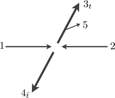
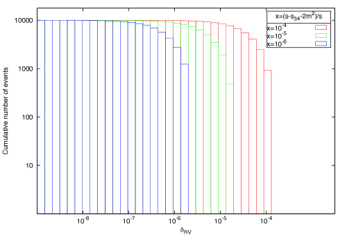
Figure 2: (a) Sketch of soft event limit. (b) Distribution of $R$ for $10^{4}$ soft phase space points with three different values of $x$

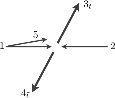
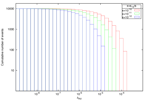
Figure 3: (a) Sketch of collinear event limit. (b) Distribution of $R$ for $10^{4}$ collinear phase space points with three different values of $x$

5 Virtual-virtual contributions to $q\bar{q}\rightarrow t\bar{t}$: the $N_{l}$ part

In this section we present the double virtual contributions to $q\bar{q}\to t\bar{t}$ proportional to $N_{l}$. We shall focus in particular in the double-virtual counter-term ${\rm d}\hat{\sigma}_{q\bar{q},NNLO,N_{l}}^{U}$ with which we construct the two-parton contribution

$$\int_{{\rm{d}}\Phi_{2\phantom{+1}}}\left[{\rm d}\hat{\sigma}_{q\bar{q},NNLO,N_{l}}^{VV}-{\rm d}\hat{\sigma}_{q\bar{q},NNLO,N_{l}}^{U}\right].$$ (42)

5.1 The virtual-virtual contributions

Following the general structure given in eq.(2), the virtual-virtual contributions can be written as

$${\rm d}\hat{\sigma}^{VV}_{q\bar{q},NNLO,N_{l}}={\cal N}_{NNLO}^{VV}N_{l}\sum_{\textrm{perms}}\int\frac{{\rm d}x_{1}}{x_{1}}\frac{{\rm d}x_{2}}{x_{2}}{\rm d}\Phi_{2}(p_{3},\ldots,p_{4};x_{1}p_{1},x_{2}p_{2})$$ (43)

$$\hskip 14.45377pt\times\delta(1-x_{1})\delta(1-x_{2})|{\cal M}^{2}_{4}(3_{Q},4_{\bar{Q}},\hat{2}_{\bar{q}},\hat{1}_{q})|^{2}\;J_{2}^{(2)}(p_{3},p_{4})\;,$$

where we have abbreviated

$$|{\cal M}^{2}_{4}(3_{Q},4_{\bar{Q}},\hat{2}_{\bar{q}},\hat{1}_{q})|^{2}=\bigg{[}2{\rm{Re}}\left({\cal M}^{2}_{q_{1}\bar{q}_{2}\rightarrow t_{3}\bar{t}_{4}}{\cal M}^{0\,\dagger}_{q_{1}\bar{q}_{2}\rightarrow t_{3}\bar{t}_{4}}\right)+|{\cal M}^{1}_{q_{1}\bar{q}_{2}\rightarrow t_{3}\bar{t}_{4}}|^{2}\bigg{]}\Bigg{|}_{N_{l}},$$ (44)

and the normalisation factor ${\cal N}_{NNLO}^{VV}$ was given in eq.(16).

For the $N_{l}$ part of the two-loop matrix element in eq.(44) we employ the analytic results of Bonciani:2008az . The “one-loop squared” term has been computed analytically in Korner:2008bn . We re-derived it ourselves, also analytically, and use our own result in our event generator. We further compared our one-loop amplitude squared with results provided by Roberto Bonciani and found full agreement.

In general, NNLO double virtual contributions contain poles of up to order four, all of which originate from the loop integrations. However, in the colour factors that we are considering in this paper, i.e. $N_{l}\,N_{c}$ and $N_{l}/N_{c}$, the deepest poles are of order three. Since at this level no partons can become unresolved, the phase space integration of ${\rm d}\hat{\sigma}^{VV}_{q\bar{q},NNLO,N_{l}}$ does not yield any additional singularities. As we shall see below, all explicit poles of the double virtual contributions are captured and cancelled by those in the subtraction term ${\rm d}\hat{\sigma}^{U}_{q\bar{q},NNLO,N_{l}}$, which, as shown in eq.(5), contains mass factorisation counter-terms as well as double real and real-virtual integrated subtraction terms.

5.2 The mass factorisation counterterm ${\rm d}\hat{\sigma}^{MF,2}$

We start the construction of the virtual-virtual subtraction term ${\rm d}\hat{\sigma}^{U}_{q\bar{q},NNLO,N_{l}}$ by deriving the mass factorisation counter-term ${\rm d}\hat{\sigma}_{q\bar{q},NNLO,N_{l}}^{MF,2}$.

In general, for a given partonic process initiated by two partons $i$ and $j$ with momenta $p_{1}$ and $p_{2}$, the mass factorisation counterterm ${\rm d}\hat{\sigma}_{ij,NNLO}^{MF,2}$ to be included at NNLO together with the double virtual matrix elements contributions reads Currie:2013vh ; GehrmannDeRidder:2011aa ; GehrmannDeRidder:2012dg ,

$${\rm d}\hat{\sigma}_{ij,NNLO}^{MF,2}(p_{1},p_{2})=-\bar{C}(\epsilon)^{2}\bigg{(}\frac{\alpha_{s}(\mu)}{2\pi}\bigg{)}^{2}\int\frac{{\rm d}x_{1}}{x_{1}}\frac{{\rm d}x_{2}}{x_{2}}\sum_{k,l}{\bf\Gamma}^{(2)}_{ij,kl}(x_{1},x_{2}){\rm d}\hat{\sigma}_{kl,LO}(x_{1}p_{1},x_{2}p_{2})$$

$$-\bar{C}(\epsilon)\frac{\alpha_{s}(\mu)}{2\pi}\int\frac{{\rm d}x_{1}}{x_{1}}\frac{{\rm d}x_{2}}{x_{2}}\sum_{k,l}{\bf\Gamma}^{(1)}_{ij,kl}(x_{1},x_{2})\Big{[}{\rm d}\hat{\sigma}_{kl,NLO}^{V}+{\rm d}\hat{\sigma}_{kl,NLO}^{MF}+\int_{1}{\rm d}\hat{\sigma}_{kl,NLO}^{S}\Big{]}(x_{1}p_{1},x_{2}p_{2}),$$

with the kernels ${\bf\Gamma}^{(1)}_{ij,kl}$ and ${\bf\Gamma}^{(2)}_{ij,kl}$ given by

$${\bf\Gamma}^{(1)}_{ij,kl}(x_{1},x_{2})=\delta_{ki}\delta(1-x_{1}){\bf\Gamma}^{(1)}_{lj}(x_{2})+\delta_{lj}\delta(1-x_{2}){\bf\Gamma}^{(1)}_{ki}(x_{1})$$ (46)

$${\bf\Gamma}^{(2)}_{ij,kl}(x_{1},x_{2})=\delta_{ki}\delta(1-x_{1}){\bf\Gamma}^{(2)}_{lj}(x_{2})+\delta_{lj}\delta(1-x_{2}){\bf\Gamma}^{(2)}_{ki}(x_{1})+{\bf\Gamma}^{(1)}_{ki}(x_{1}){\bf\Gamma}^{(1)}_{lj}(x_{2}).$$ (47)

To simplify the construction of the double virtual subtraction term ${\rm d}\hat{\sigma}_{NNLO}^{U}$, the splitting kernel ${\bf\Gamma}^{(2)}_{ij,kl}$ can be written as suggested in Currie:2013vh as

$${\bf\Gamma}_{ij;kl}^{(2)}(x_{1},x_{2})=\overline{{\bf\Gamma}}_{ij;kl}^{(2)}(x_{1},x_{2})-\frac{\beta_{0}}{\epsilon}{\bf\Gamma}_{ij;kl}^{(1)}(x_{1},x_{2})+\frac{1}{2}\big{[}{\bf\Gamma}_{ij;ab}^{(1)}\otimes{\bf\Gamma}_{ab;kl}^{(1)}\big{]}(x_{1},x_{2}),$$ (48)

such that,

$$\overline{{\bf\Gamma}}_{ij;kl}^{(2)}(x_{1},x_{2})=\overline{{\bf\Gamma}}_{ik}^{(2)}(x_{1})\delta_{jl}\delta(1-x_{2})+\overline{{\bf\Gamma}}_{jl}^{(2)}(x_{2})\delta_{ik}\delta(1-x_{1}).$$ (49)

The kernel $\overline{{\bf\Gamma}}_{ij}^{(2)}(z)$ is related to the usual Altarelli-Parisi splitting functions Altarelli:1977zs as

$$\overline{{\bf\Gamma}}_{ij}^{(2)}(x) = -\frac{1}{2\epsilon}\bigg{(}{\bf P}_{ij}^{1}(x)+\frac{\beta_{0}}{\epsilon}{\bf P}_{ij}^{0}(x).\bigg{)}.$$ (50)

For the partonic process $q\bar{q}\to t\bar{t}$, the part of the mass factorisation counter-term ${\rm d}\hat{\sigma}^{MF,2}_{q\bar{q},NNLO}$ that is proportional to $N_{l}$ reads

$${\rm d}\hat{\sigma}_{q\bar{q},NNLO,N_{l}}^{MF,2}(p_{1},p_{2})=$$

$$\hskip 15.89948ptN_{l}\bigg{[}-\bar{C}(\epsilon)\frac{\alpha_{s}(\mu)}{2\pi}\int\frac{{\rm d}x_{1}}{x_{1}}\frac{{\rm d}x_{2}}{x_{2}}{\bf\Gamma}_{qq;qq}^{(1)}(x_{1},x_{2}){\rm d}\hat{\sigma}_{q\bar{q},NLO,N_{l}}^{V}(x_{1}p_{1},x_{2}p_{2})$$

$$\hskip 36.135pt-\bar{C}(\epsilon)^{2}\bigg{(}\frac{\alpha_{s}(\mu)}{2\pi}\bigg{)}^{2}\int\frac{{\rm d}x_{1}}{x_{1}}\frac{{\rm d}x_{2}}{x_{2}}{\bf\Gamma}_{qq;qq}^{(2),[N_{l}]}(x_{1},x_{2}){\rm d}\hat{\sigma}_{q\bar{q},LO}(x_{1}p_{1},x_{2}p_{2})\bigg{]},$$

where ${\bf\Gamma}_{qq;qq}^{(2),[N_{l}]}$ and ${\rm d}\hat{\sigma}_{q\bar{q},NLO,N_{l}}^{V}$ denote the pieces proportional to $N_{l}$ in ${\bf\Gamma}_{qq;qq}^{(2)}$ and ${\rm d}\hat{\sigma}_{q\bar{q},NLO}^{V}$ respectively. Moreover, ${\rm d}\hat{\sigma}_{q\bar{q},LO}$ is the leading order partonic cross section for the process $q\bar{q}\to t\bar{t}$.

Trading ${\bf\Gamma}^{(2)}_{qq;qq}$ for $\overline{\bf\Gamma}^{(2)}_{qq;qq}$ in eq.(48), ${\rm d}\hat{\sigma}^{MF,2}_{q\bar{q},NNLO}$ can be compactly written as the sum of

$${\rm d}\hat{\sigma}^{MF,2a}_{q\bar{q},NNLO}(p_{1},p_{2})=-N_{l}\,\bar{C}(\epsilon)\,\frac{\alpha_{s}(\mu)}{2\pi}\int\frac{{\rm d}x_{1}}{x_{1}}\frac{{\rm d}x_{2}}{x_{2}}{\bf\Gamma}_{qq;qq}^{(1)}(x_{1},x_{2})$$

$$\hskip 21.68121pt\times\bigg{[}{\rm d}\hat{\sigma}_{q\bar{q},NLO,N_{l}}^{V}(x_{1}p_{1},x_{2}p_{2})-\bar{C}(\epsilon)\frac{\alpha_{s}(\mu)}{2\pi}\frac{b_{0,F}}{\epsilon}{\rm d}\hat{\sigma}_{qq,LO}(x_{1}p_{1},x_{2}p_{2})\bigg{]}$$ (52)

and

$${\rm d}\hat{\sigma}^{MF,2c}_{q\bar{q},NNLO}(p_{1},p_{2})=-N_{l}\,\bar{C}(\epsilon)^{2}\bigg{(}\frac{\alpha_{s}(\mu)}{2\pi}\bigg{)}^{2}\int\frac{{\rm d}x_{1}}{x_{1}}\frac{{\rm d}x_{2}}{x_{2}}\overline{\bf\Gamma}_{qq;qq}^{(2),[N_{l}]}(x_{1},x_{2}){\rm d}\hat{\sigma}_{q\bar{q},LO}(x_{1}p_{1},x_{2}p_{2}),$$ (53)

with the kernels ${\bf\Gamma}_{qq;qq}^{(1)}$ and $\overline{\bf\Gamma}_{qq;qq}^{(2),[N_{l}]}$ constructed as in eqs.(46-48) using the expressions given in the appendix of Currie:2013vh .

Note finally that the mass factorisation counter-term denoted in Currie:2013vh as ${\rm d}\hat{\sigma}^{MF,2b}$, which is necessary in the most general cases, is absent here. This is due to the fact that the one-loop kernel ${\bf\Gamma}_{qq;qq}^{(1)}$ does not contain any terms proportional to $N_{l}$.

5.3 The virtual-virtual subtraction term ${\rm d}\hat{\sigma}^{U}$

In addition to the mass factorisation counter-term derived above, the virtual-virtual subtraction term ${\rm d}\hat{\sigma}_{NNLO}^{U}$ contains in general contributions originated from the integrated double real and real-virtual subtraction terms. In the present case, it is given by

$${\rm d}\hat{\sigma}^{U}_{q\bar{q},NNLO,N_{l}}=-\int_{2}{\rm d}\hat{\sigma}^{S,b\>4}_{q\bar{q},NNLO,N_{l}}-{\rm d}\hat{\sigma}^{MF,2}_{q\bar{q},NNLO,N_{l}}-\int_{1}{\rm d}\hat{\sigma}^{VS,a}_{q\bar{q},NNLO,N_{l}}-\int_{1}{\rm d}\hat{\sigma}^{VS,d}_{q\bar{q},NNLO,N_{l}}.$$ (54)

The integrated double real subtraction term $\int_{2}{\rm d}\hat{\sigma}^{S,b\>4}_{q\bar{q},NNLO,N_{l}}$ in the equation above is obtained by integrating the four-parton B-type antennae in the subtraction term ${\rm d}\hat{\sigma}^{S,b\>4}_{q\bar{q},NNLO,N_{l}}$ given in eq.(A). Doing so we find

$$\int_{2}{\rm d}\hat{\sigma}^{S,b\>4}_{q\bar{q},NNLO,N_{l}}={\cal N}_{NNLO}^{VV}N_{l}\int\frac{{\rm d}x_{1}}{x_{1}}\frac{{\rm d}x_{2}}{x_{2}}{\rm d}\Phi_{2}(p_{3},p_{4};x_{1}p_{1},x_{2}p_{2})$$

$$\times\bigg{\{}N_{c}\bigg{[}{\cal B}^{0}_{q,Qq^{\prime}\bar{q^{\prime}}}(\epsilon,s_{\bar{1}3},x_{1},x_{2})+{\cal B}^{0}_{q,Qq^{\prime}\bar{q^{\prime}}}(\epsilon,s_{\bar{2}4},x_{2},x_{1})\bigg{]}$$

$$\hskip 5.78172pt+\frac{1}{N_{c}}\bigg{[}2{\cal B}^{0}_{q,Qq^{\prime}\bar{q^{\prime}}}(\epsilon,s_{\bar{2}3},x_{1},x_{2})+2{\cal B}^{0}_{q,Qq^{\prime}\bar{q^{\prime}}}(\epsilon,s_{\bar{1}4},x_{2},x_{1})$$

$$\hskip 27.10124pt-2{\cal B}^{0}_{q,Qq^{\prime}\bar{q^{\prime}}}(\epsilon,s_{\bar{1}3},x_{1},x_{2})-2{\cal B}^{0}_{q,Qq^{\prime}\bar{q^{\prime}}}(\epsilon,s_{\bar{2}4},x_{2},x_{1})\phantom{\bigg{[}}$$

$$\hskip 27.10124pt-{\cal B}^{0}_{Qq\bar{q}\hat{Q}}(\epsilon,s_{34},x_{1},x_{2})-{\cal B}^{0}_{q\bar{q},q^{\prime}\bar{q^{\prime}}}(\epsilon,s_{\bar{1}\bar{2}},x_{1},x_{2})\bigg{]}\bigg{\}}|{\cal M}^{0}_{4}(3_{Q},4_{\bar{Q}},\hat{\bar{2}}_{\bar{q}},\hat{\bar{1}}_{q})|^{2}J_{2}^{(2)}(p_{3},p_{4})$$

Similarly, the integrated real-virtual subtraction terms $\int_{1}{\rm d}\hat{\sigma}^{VS,a}_{q\bar{q},NNLO,N_{l}}$ and $\int_{1}{\rm d}\hat{\sigma}^{VS,d}_{q\bar{q},NNLO,N_{l}}$ are obtained from eqs.(4.2) and (4.2.3) by integrating the tree-level and one-loop three parton antennae over their corresponding phase space. We obtain

$$\int_{1}{\rm d}\hat{\sigma}_{q\bar{q},NNLO,N_{l}}^{VS,a}={\cal N}_{NNLO}^{VV}\,N_{l}\int\frac{{\rm d}x_{1}}{x_{1}}\frac{{\rm d}x_{2}}{x_{2}}{\rm d}\Phi_{2}(p_{3},p_{4};x_{1}p_{1},x_{2}p_{2})$$

$$\times\bigg{\{}N_{c}\bigg{[}\bigg{(}{\cal A}^{1,l}_{q,Qg}(\epsilon,s_{\bar{1}3},x_{1},x_{2})+{\cal A}^{1,l}_{q,Qg}(\epsilon,s_{\bar{2}4},x_{2},x_{1})\bigg{)}|{\cal M}^{0}_{4}(3_{Q},4_{\bar{Q}},\hat{\bar{2}}_{\bar{q}},\hat{\bar{1}}_{q})|^{2}$$

$$\hskip 27.10124pt+\bigg{(}{\cal A}^{0}_{q,Qg}(\epsilon,s_{\bar{1}3},x_{1},x_{2})+{\cal A}^{0}_{q,Qg}(\epsilon,s_{\bar{2}4},x_{2},x_{1})\bigg{)}|{\cal M}_{4}^{[l]}(3_{Q},4_{\bar{Q}},\hat{\bar{2}}_{\bar{q}},\hat{\bar{1}}_{q})|^{2}\bigg{]}$$

$$\hskip 5.78172pt+\frac{1}{N_{c}}\bigg{[}\bigg{(}2{\cal A}^{1,l}_{q,Qg}(\epsilon,s_{\bar{2}3},x_{2},x_{1})+2{\cal A}^{1,l}_{q,Qg}(\epsilon,s_{\bar{1}4},x_{1},x_{2})$$

$$\hskip 36.135pt-2{\cal A}^{1,l}_{q,Qg}(\epsilon,s_{\bar{1}3},x_{1},x_{2})-2{\cal A}^{1,l}_{q,Qg}(\epsilon,s_{\bar{2}4},x_{2},x_{1})\phantom{\bigg{(}}$$

$$\hskip 36.135pt-2{\cal A}^{1,l}_{Qg\bar{Q}}(\epsilon,s_{34},x_{1},x_{2})-2{\cal A}^{1,l}_{q\bar{q},g}(\epsilon,s_{\bar{1}\bar{2}},x_{1},x_{2})\bigg{)}|{\cal M}^{0}_{4}(3_{Q},4_{\bar{Q}},\hat{\bar{2}}_{\bar{q}},\hat{\bar{1}}_{q})|^{2}$$

$$\hskip 27.46295pt+\bigg{(}2{\cal A}^{0}_{q,Qg}(\epsilon,s_{\bar{2}3},x_{2},x_{1})+2{\cal A}^{0}_{q,Qg}(\epsilon,s_{\bar{1}4},x_{1},x_{2})$$

$$\hskip 36.135pt-2{\cal A}^{0}_{q,Qg}(\epsilon,s_{\bar{1}3},x_{1},x_{2})-2{\cal A}^{0}_{q,Qg}(\epsilon,s_{\bar{2}4},x_{2},x_{1})\phantom{\bigg{(}}$$

$$\hskip 36.135pt-2{\cal A}^{0}_{Qg\bar{Q}}(\epsilon,s_{34},x_{1},x_{2})-2{\cal A}^{0}_{q\bar{q},g}(\epsilon,s_{\bar{1}\bar{2}},x_{1},x_{2})\bigg{)}|{\cal M}_{4}^{[l]}(3_{Q},4_{\bar{Q}},\hat{\bar{2}}_{\bar{q}},\hat{\bar{1}}_{q})|^{2}\bigg{]}\bigg{\}}J_{2}^{(2)}(p_{3},p_{4}),$$

while for the integrated form of renormalisation scale dependent subtraction term we get

$$\int_{1}{\rm d}\hat{\sigma}_{q\bar{q},NNLO,N_{l}}^{VS,d}={\cal N}_{NNLO}^{VV}\,N_{l}\,b_{0,F}\int\frac{{\rm d}x_{1}}{x_{1}}\frac{{\rm d}x_{2}}{x_{2}}{\rm d}\Phi_{2}(p_{3},p_{4};x_{1}p_{1},x_{2}p_{2})|{\cal M}^{0}_{4}(3_{Q},4_{\bar{Q}},\hat{\bar{2}}_{\bar{q}},\hat{\bar{1}}_{q})|^{2}$$

$$\times\bigg{\{}N_{c}\bigg{[}\bigg{(}\log\left(\frac{\mu^{2}}{s_{\bar{1}3}}\right){\cal A}^{0}_{\hat{q},Qg}(\epsilon,s_{\bar{1}3},x_{1},x_{2})+\log\left(\frac{\mu^{2}}{s_{\bar{2}4}}\right){\cal A}^{0}_{\hat{q},Qg}(\epsilon,s_{\bar{2}4},x_{2},x_{1})\bigg{)}\bigg{]}$$

$$\hskip 5.42003pt+\frac{1}{N_{c}}\bigg{[}\bigg{(}2\log\left(\frac{\mu^{2}}{s_{\bar{2}3}}\right){\cal A}^{0}_{\hat{q},Qg}(\epsilon,s_{\bar{2}3},x_{2},x_{1})+2\log\left(\frac{\mu^{2}}{s_{\bar{1}4}}\right){\cal A}^{0}_{\hat{q},Qg}(\epsilon,s_{\bar{1}4},x_{1},x_{2})$$

$$\hskip 34.32869pt-2\log\left(\frac{\mu^{2}}{s_{\bar{1}3}}\right){\cal A}^{0}_{\hat{q},Qg}(\epsilon,s_{\bar{1}3},x_{1},x_{2})-2\log\left(\frac{\mu^{2}}{s_{\bar{2}4}}\right){\cal A}^{0}_{\hat{q},Qg}(\epsilon,s_{\bar{2}4},x_{2},x_{1})$$

$$\hskip 34.32869pt-\log\left(\frac{\mu^{2}}{s_{34}}\right){\cal A}^{0}_{Q\bar{Q}g}(\epsilon,s_{34},x_{1},x_{2})-\log\left(\frac{\mu^{2}}{s_{\bar{1}\bar{2}}}\right){\cal A}^{0}_{\hat{q}\hat{\bar{q}},g}(\epsilon,s_{\bar{1}\bar{2}},x_{2},x_{1})\bigg{)}\bigg{]}\bigg{\}}J_{2}^{(2)}(p_{3},p_{4}).$$

With the explicit expressions obtained for the integrated antennae, one can show analytically that

$${\cal P}oles\left({\rm d}\hat{\sigma}_{NNLO}^{VV}-{\rm d}\hat{\sigma}_{NNLO}^{U}\ \right)=0$$ (58)

demonstrating that we have correctly implemented all the subtractions terms at real-real, real-virtual and virtual-virtual levels in leading ($N_{l}N_{c}$) and subleading-colour ($N_{l}/N_{c}$) contributions for the parton-level process $q\bar{q}\to t\bar{t}$.

This pole cancellation provides furthermore a crucial check on the integrated forms of the massless and massive four-parton B-type antennae derived in Abelof:2012he ; Bernreuther:2011jt ; Boughezal:2010mc and of the correct implementation of the one-and two-loop massive amplitudes. Finally, it also provides a proof that the massive extension of the NNLO antenna formalism can be used to extract and cancel the infrared singularities of the top-antitop pair production cross section evaluated at the NNLO level, enabling the construction of a fully differential event generator.

6 Numerical results: NNLO differential distributions

With the double real counter-terms derived in Abelof:2011ap and recalled in appendix A together with the real-virtual and virtual-virtual subtraction terms presented above in sections 4 and 5, we developed a Monte Carlo parton-level event generator based on the set up of eq.(2). This program, written in Fortran following the structure of the program developed in GehrmannDeRidder:2013mf for the calculation of the di-jet hadronic cross section at NNLO, allows us to produce the first differential distributions for top pair production including exact NNLO results, namely the ${\cal O}(\alpha_{s}^{4})$ corrections to the $q\bar{q}\rightarrow t\bar{t}$ process proportional to the number of light quark flavors $N_{l}$.

In this section we present differential distributions in the top quark transverse momentum, the top quark rapidity, as well as in the rapidity and invariants mass of the top-antitop system. We consider the $q\bar{q}$ initiated process only, convoluted with parton distribution functions (PDFs) corresponding to proton-proton collisions, at leading order, next-to-leading order, and next-to-next-to-leading order. The next-to-next-to leading order results denoted as NNLO ($N_{l}$) in the figures 4-7 presented in this section are the sum of the full NLO corrections and the purely fermionic NNLO corrections to $q\bar{q}\rightarrow t\bar{t}$ discussed in this paper.

We employ a hadronic center-of-mass energy $\sqrt{s}=7$ TeV, a value of the top quark mass given by $m_{t}=173.5$ GeV, and the PDF sets MSTW2008LO90CL, MSTW2008NLO90CL and MSTW2008NNLO90CL for the computations at LO, NLO and NNLO respectively Martin:2009iq . We set the factorisation and renormalisation scales to be equal to the top quark mass $\mu_{R}=\mu_{F}=m_{t}$.

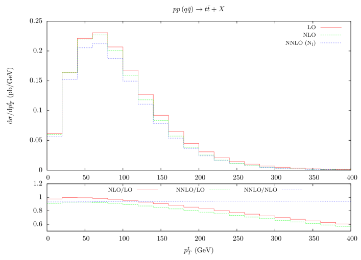
Figure 4: Transverse momentum distribution of a single top quark ${\rm d}\sigma/{\rm d}p_{T}^{t}$ for $\sqrt{s}=7$ TeV at LO (red), NLO (green), and NNLO (blue). The lower panel shows the ratios of LO, NLO and NNLO cross sections.

In figure 4 we present the inclusive $t\bar{t}$ cross section as a function of the top quark transverse momentum $p_{T}^{t}$ at LO, NLO, and NNLO together with the corresponding $k$-factors. From the NNLO/NLO ratio we see that the NNLO contributions proportional to $N_{l}$ decrease the cross section by $6-7\%$ depending on the value of the transverse momentum $p_{T}^{t}$ compared to the NLO result.

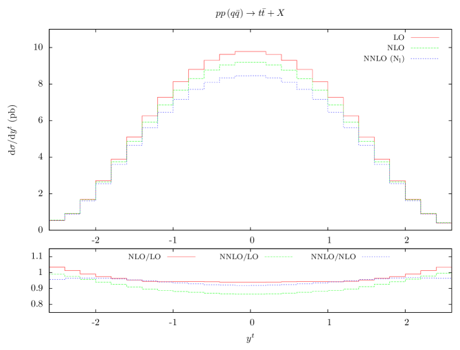
Figure 5: Rapidity distribution of a single top quark ${\rm d}\sigma/{\rm d}y^{t}$ for $\sqrt{s}=7$ TeV at LO (red), NLO (green), and NNLO (blue). The lower panel shows the ratios of LO, NLO and NNLO cross sections.

In figure 5 we show the inclusive $t\bar{t}$ cross section as a function of the top quark rapidity $y^{t}$ at LO, NLO, and NNLO with the corresponding $k$-factors in the lower panel. The NNLO/NLO ratio shows that the NNLO contributions proportional to $N_{l}$ decrease the cross section by $8\%$ in the central region and $5\%$ in the forward and backward regions.

Figure 6: Rapidity distribution of the top-antitop system ${\rm d}\sigma/{\rm d}y^{t\bar{t}}$ for $\sqrt{s}=7$ TeV at LO (red), NLO (green), and NNLO (blue). The lower panel shows the ratios of LO, NLO and NNLO cross sections.

Figure 6 contains the inclusive $t\bar{t}$ cross section as a function of the rapidity of the top-antitop system $y^{t\bar{t}}$ at LO, NLO and NNLO together with their corresponding $k$-factors. Once again we note an overall decrease in the cross section at NNLO, ranging from $2.5$ to $8.5\%$ with respect to the NLO result depending on the rapidity region considered.

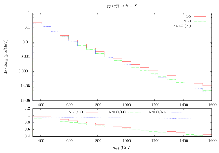
Figure 7: Invariant mass distribution of the top-antitop system ${\rm d}\sigma/{\rm d}m_{t\bar{t}}$ for $\sqrt{s}=7$ TeV at LO (red), NLO (green), and NNLO (blue). The lower panel shows the ratios of LO, NLO and NNLO cross sections.

In figure 7 we present the cross section as a function of the invariant mass of the $t\bar{t}$ system at LO, NLO and NNLO, with all three ratios in the lower panel. As can be seen from the NNLO/NLO ratio, the NNLO corrections proportional to the number of light quark flavours $N_{l}$ decrease the cross section over the entire $m_{t\bar{t}}$ spectrum considered. The decrease ranges from $6.5\%$ in the low invariant mass region to almost $10\%$ in the high invariant mass region.

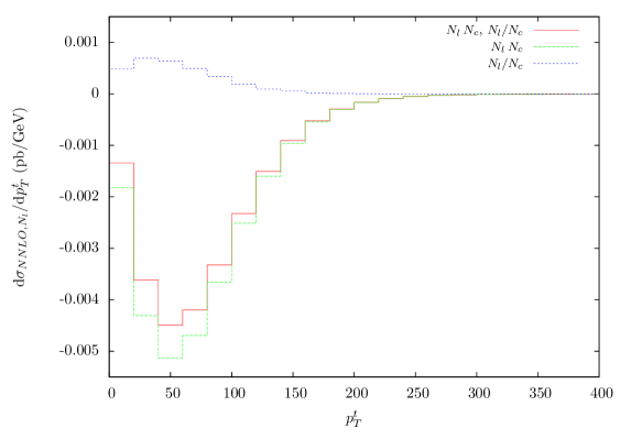
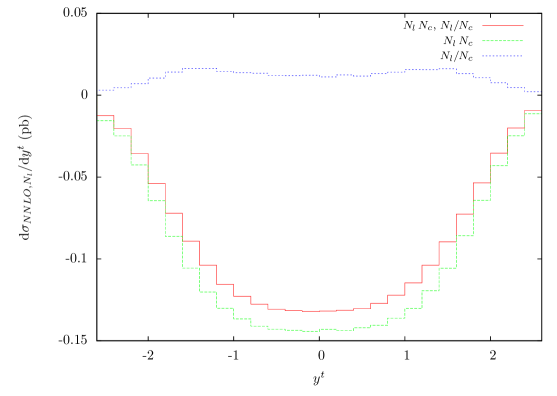
Figure 8: Individual NNLO contributions due to the colour factors $N_{l}\,N_{c}$ and $N_{l}/N_{c}$ as a function of (a) the top quark transverse momentum, (b) the top quark rapidity.

Naïve power counting suggests that the leading-colour NNLO contributions considered in this paper, i.e. the pieces proportional to $N_{l}\,N_{c}$ should approximately account for $90\%$ of the NNLO corrections, with the remainder being given by the subleading-colour contributions, proportional to $N_{l}/N_{c}$. At the level of the total cross section we find that the subleading-colour pieces are opposite in sign to the leading-colour and represent $13\%$ of the full result, in agreement with this naïve power counting expectation.

In order to assess the impact of the subleading-colour contributions, we studied the NNLO corrections proportional to $N_{l}N_{c}$ and $N_{l}/N_{c}$ separately as a function of the top quark transverse momentum and rapidity. The results of these studies are shown in figures 8(a) and 8(b). We find that the subleading-colour piece has a different shape and sign than the leading-colour part, and contributes more significantly in the forward and backwards regions and less when the top quark is more centrally produced. In particular, in the $p_{T}^{t}$ spectrum of figure 8(a) we find that at low transverse momenta, the size of the $N_{l}/N_{c}$ colour factor is of approximately $30\%$ of the full colour result, while at high transverse momenta its contribution is negligible.

As a check of our numerical results, we compared the value of the total NNLO correction proportional to $N_{l}$ with the result presented in Baernreuther:2012ws . In order to perform this check we had to incorporate to our calculation the NNLO contributions proportional to $N_{h}N_{l}$, with $N_{h}$ the number of heavy quark flavours, since those are included in the coefficient function $F_{1}(\beta)$ of Baernreuther:2012ws . These contributions are rather simple, as they only enter at the double virtual level, and they are finite. We employed the two-loop matrix elements derived in Bonciani:2008az , and computed the square of the one-loop matrix elements ourselves. With the same input parameters and PDF sets used throughout the present section, we find that the total NNLO correction to top pair production proportional to $N_{l}$ in the $q\bar{q}$ channel is $-0.5780$ pb, whereas with the coefficient function $F_{1}(\beta)$ of Baernreuther:2012ws we obtain $-0.5822$ pb. These two results agree within less that $1\%$, which represents a very strong check of both completely independent calculations.

7 Conclusions

In this paper we presented the ${\cal O}(\alpha_{s}^{4})$ light fermionic corrections to the partonic process $q\bar{q}\to t\bar{t}$. Those corrections are of three types: virtual-virtual, real-virtual and double real, with two, three and four particles in the final state respectively. While the ultraviolet divergencies are removed by renormalisation, the infrared singularities are treated using the massive extension of the NNLO antenna formalism.

The double real corrections had been derived in Abelof:2011ap . In this paper we presented the real-virtual and virtual-virtual contributions and derived their related subtraction terms explicitly. We showed that the real-virtual subtraction terms correctly approximate the real-virtual matrix elements in all their singular limits. Furthermore, combined with the integrated forms of the subtraction terms, we show analytically that all explicit infrared singularities are cancelled both at real-virtual and at the virtual-virtual levels. This analytic pole cancellation provides us with a very strong check on the correctness of our result and on the applicability of the antenna subtraction method to reactions involving massive final states.

The NNLO results of this paper are implemented in a Monte Carlo parton-level generator providing full kinematical information on an event-by event basis. This program, written in Fortran, allowed us to produce NNLO differential distributions for top pair production in the partonic channel under consideration for the first time. We studied the impact of the NNLO corrections proportional to $N_{l}$ for distributions in $p_{T}$ and rapidity of the top quark as well as in the rapidity and invariant mass of the $t\bar{t}$ system and found that those corrections are substantial. They reduce the cross section compared to the NLO results, with the reduction varying considerably over the phase space. We also assessed the separate sizes of the leading and subleading-colour $N_{l}$ contributions finding that they have opposite signs, and that, at the level of the total cross section, the subleading-colour part contributes with $13\%$. Its importance, however, varies substantially over different regions of phase space. It can be as high as $30\%$ for low transverse momenta of the top quark, and negligible for high transverse momenta.

The results presented in this paper can be regarded as a major step towards the computation of the complete cross section of top pair production including all partonic channels in fully differential form. For the first time, we have presented exact NNLO ($N_{l}$) corrections to one partonic channel in this process and produced NNLO differential distributions. Further work will include the computation of all remaining partonic channels.

Appendix A The double real subtraction term for $q\bar{q}\rightarrow t\bar{t}$: the $N_{l}$ part

The double real corrections to the process $q\bar{q}\rightarrow t\bar{t}$ proportional to the number of light quark flavours are due to the tree-level partonic process $q\bar{q}\rightarrow t\bar{t}q^{\prime}\bar{q}^{\prime}$. We derived the corresponding subtraction terms in Abelof:2011ap and found that only two pieces are needed, namely $ds^{S,a}_{q\bar{q},NNLO,N_{l}}$ and ${\rm d}\hat{\sigma}^{S,b}_{q\bar{q},NNLO,N_{l}}$. The subtraction term $ds^{S,a}_{q\bar{q},NNLO,N_{l}}$ capturing the single unresolved limits of the real-real contributions read

$${\rm d}\hat{\sigma}^{S,a}_{q\bar{q},NNLO,N_{l}}={\cal N}_{NNLO}^{RR,q\bar{q}}\,N_{l}\,{\rm d}\Phi_{4}(p_{3},p_{4},p_{5},p_{6};p_{1},p_{2})$$

$$\times\bigg{\{}N_{c}\bigg{[}\frac{1}{2}E_{3}^{0}(3_{Q},5_{q^{\prime}},6_{\bar{q}^{\prime}})\bigg{(}|{\cal M}^{0}_{5}((\widetilde{35})_{Q},\hat{1}_{q};;\hat{2}_{\bar{q}},(\widetilde{56})_{g},4_{\bar{Q}})|^{2}$$

$$\>\>\>\>\>\>\>\>\>\>\>\>\>\>\>\>\>\>\>\>\>\>\>\>\>\>\>\>\>+|{\cal M}^{0}_{5}((\widetilde{35})_{Q},(\widetilde{56})_{g},\hat{1}_{q};;\hat{2}_{\bar{q}},4_{\bar{Q}})|^{2}\bigg{)}J_{2}^{(3)}(p_{\widetilde{35}},p_{4},p_{\widetilde{56}})$$

$$\>\>\>\>\>\>\>\>\>\>\>+\frac{1}{2}E_{3}^{0}(4_{\bar{Q}},5_{q^{\prime}},6_{\bar{q}^{\prime}})\bigg{(}|{\cal M}^{0}_{5}(3_{Q},\hat{1}_{q};;\hat{2}_{\bar{q}},(\widetilde{56})_{g},(\widetilde{45})_{\bar{Q}})|^{2}$$

$$\>\>\>\>\>\>\>\>\>\>\>\>\>\>\>\>\>\>\>\>\>\>\>\>\>\>\>\>\>+|{\cal M}^{0}_{5}(3_{Q},(\widetilde{56})_{g},\hat{1}_{q};;\hat{2}_{\bar{q}},(\widetilde{45})_{\bar{Q}})|^{2}\bigg{)}J_{2}^{(3)}(p_{3},p_{\widetilde{45}},p_{\widetilde{56}})\bigg{]}$$

$$\>\>+\frac{1}{N_{c}}\bigg{[}\frac{1}{2}E_{3}^{0}(3_{Q},5_{q^{\prime}},6_{\bar{q}^{\prime}})\bigg{(}|{\cal M}^{0}_{5}((\widetilde{35})_{Q},4_{\bar{Q}};;\hat{2}_{\bar{q}},(\widetilde{56})_{g},\hat{1}_{q})|^{2}$$

$$\>\>\>\>\>\>\>\>\>\>\>\>\>\>\>\>\>\>\>\>\>\>\>\>\>\>\>\>\>\>\>\>\>\>\>\>\>\>\>\>\>\>\>\>\>\>+|{\cal M}^{0}_{5}((\widetilde{35})_{Q},(\widetilde{56})_{g},4_{\bar{Q}};;\hat{2}_{\bar{q}},\hat{1}_{q})|^{2}$$

$$\>\>\>\>\>\>\>\>\>\>\>\>\>\>\>\>\>\>\>\>\>\>\>\>\>\>\>\>\>\>\>\>\>\>\>\>\>\>\>\>\>\>\>\>\>\>-2|{\cal M}^{0}_{5}((\widetilde{35})_{Q},4_{\bar{Q}},\hat{2}_{\bar{q}},\hat{1}_{q},(\widetilde{56})_{\gamma})|^{2}\bigg{)}J_{2}^{(3)}(p_{\widetilde{35}},p_{4},p_{\widetilde{56}})$$

$$\>\>\>\>\>\>\>\>\>\>\>+\frac{1}{2}E_{3}^{0}(4_{\bar{Q}},5_{q^{\prime}},6_{\bar{q}^{\prime}})\bigg{(}|{\cal M}^{0}_{5}(3_{Q},(\widetilde{45})_{\bar{Q}};;\hat{2}_{\bar{q}},(\widetilde{56})_{g},\hat{1}_{q})|^{2}$$

$$\>\>\>\>\>\>\>\>\>\>\>\>\>\>\>\>\>\>\>\>\>\>\>\>\>\>\>\>\>\>\>\>\>\>\>\>\>\>\>\>\>\>\>\>\>\>+|{\cal M}^{0}_{5}(3_{Q},(\widetilde{56})_{g},(\widetilde{45})_{\bar{Q}};;\hat{2}_{\bar{q}},\hat{1}_{q})|^{2}$$

$$\>\>\>\>\>\>\>\>\>\>\>\>\>\>\>\>\>\>\>\>\>\>\>\>\>\>\>\>\>\>\>\>\>\>\>\>\>\>\>\>\>\>\>\>\>\>-2|{\cal M}^{0}_{5}(3_{Q},(\widetilde{45})_{\bar{Q}},\hat{2}_{\bar{q}},\hat{1}_{q},(\widetilde{56})_{\gamma})|^{2}\bigg{)}J_{2}^{(3)}(p_{3},p_{\widetilde{45}},p_{\widetilde{56}})\bigg{]}\bigg{\}}.$$

${\rm d}\hat{\sigma}^{S,b}_{q\bar{q},NNLO,N_{l}}$ captures the double unresolved limit. It reads

$${\rm d}\hat{\sigma}^{S,b}_{q\bar{q},NNLO,N_{l}}={\cal N}_{NNLO}^{RR,q\bar{q}}\,N_{l}\,{\rm d}\Phi_{4}(p_{3},p_{4},p_{5},p_{6};p_{1},p_{2})$$

$$\times\bigg{\{}N_{c}\bigg{[}\bigg{(}B_{4}^{0}(3_{Q},6_{\bar{q}^{\prime}},5_{q^{\prime}},\hat{1}_{q})-\frac{1}{2}E_{3}^{0}(3_{Q},5_{q^{\prime}},6_{\bar{q}^{\prime}})A_{3}^{0}((\widetilde{35})_{Q},(\widetilde{56})_{g},\hat{1}_{q})$$

$$\>\>\>\>\>\>\>\>\>\>\>\>\>\>\>-\frac{1}{2}E_{3}^{0}(4_{\bar{Q}},5_{q^{\prime}},6_{\bar{q}^{\prime}})A_{3}^{0}(3_{Q},(\widetilde{56})_{g},\hat{1}_{q})\bigg{)}|{\cal M}^{0}_{4}((\widetilde{356})_{Q},4_{\bar{Q}},\hat{2}_{\bar{q}},\hat{\bar{1}}_{q})|^{2}J_{2}^{(2)}(p_{\widetilde{356}},p_{4})$$

$$\>\>\>\>\>\>\>\>\>\>\>+\bigg{(}B_{4}^{0}(4_{\bar{Q}},5_{q^{\prime}},6_{\bar{q}^{\prime}},\hat{2}_{\bar{q}})-\frac{1}{2}E_{3}^{0}(3_{Q},5_{q^{\prime}},6_{\bar{q}^{\prime}})A_{3}^{0}(4_{\bar{Q}},(\widetilde{56})_{g},\hat{2}_{\bar{q}})$$

$$\>\>\>\>\>\>\>\>\>\>\>\>\>\>\>-\frac{1}{2}E_{3}^{0}(4_{\bar{Q}},5_{q^{\prime}},6_{\bar{q}^{\prime}})A_{3}^{0}((\widetilde{45})_{\bar{Q}},(\widetilde{56})_{g},\hat{2}_{\bar{q}})\bigg{)}|{\cal M}^{0}_{4}(3_{Q},(\widetilde{456})_{\bar{Q}},\hat{\bar{2}}_{\bar{q}},\hat{1}_{q})|^{2}J_{2}^{(2)}(p_{3},p_{\widetilde{456}})\bigg{]}$$

$$-\frac{1}{N_{c}}\bigg{[}\bigg{(}B_{4}^{0}(3_{Q},6_{\bar{q}^{\prime}},5_{q^{\prime}},4_{\bar{Q}})-\frac{1}{2}E_{3}^{0}(3_{Q},5_{q^{\prime}},6_{\bar{q}^{\prime}})A_{3}^{0}((\widetilde{35})_{Q},(\widetilde{56})_{g},4_{\bar{Q}})$$

$$\>\>\>\>\>\>\>\>\>\>\>\>\>\>-\frac{1}{2}E_{3}^{0}(4_{\bar{Q}},5_{q^{\prime}},6_{\bar{q}^{\prime}})A_{3}^{0}(3_{Q},(\widetilde{56})_{g},(\widetilde{45})_{\bar{Q}})\bigg{)}|{\cal M}^{0}_{4}((\widetilde{356})_{Q},(\widetilde{456})_{\bar{Q}},\hat{2}_{\bar{q}},\hat{1}_{q})|^{2}J_{2}^{(2)}(p_{\widetilde{356}},p_{\widetilde{456}})$$

$$\>\>\>\>\>\>\>\>\>+\bigg{(}B_{4}^{0}(\hat{2}_{\bar{q}},6_{\bar{q}^{\prime}},5_{q^{\prime}},\hat{1}_{q})-\frac{1}{2}E_{3}^{0}(3_{Q},5_{q^{\prime}},6_{\bar{q}^{\prime}})A_{3}^{0}(\hat{2}_{\bar{q}},(\widetilde{56})_{g},\hat{1}_{q})$$

$$\>\>\>\>\>\>\>\>\>\>\>\>\>\>-\frac{1}{2}E_{3}^{0}(4_{\bar{Q}},5_{q^{\prime}},6_{\bar{q}^{\prime}})A_{3}^{0}(\hat{2}_{\bar{q}},(\widetilde{56})_{g},\hat{1}_{q})\bigg{)}|{\cal M}^{0}_{4}(\tilde{3}_{Q},\tilde{4}_{\bar{Q}},\hat{\bar{2}}_{\bar{q}},\hat{\bar{1}}_{q})|^{2}J_{2}^{(2)}(\tilde{p}_{3},\tilde{p}_{4})$$

$$\>\>\>\>\>\>\>\>\>+2\bigg{(}B_{4}^{0}(3_{Q},6_{\bar{q}^{\prime}},5_{q^{\prime}},\hat{1}_{q})-\frac{1}{2}E_{3}^{0}(3_{Q},5_{q^{\prime}},6_{\bar{q}^{\prime}})A_{3}^{0}((\widetilde{35})_{Q},(\widetilde{56})_{g},\hat{1}_{q})$$

$$\>\>\>\>\>\>\>\>\>\>\>\>\>\>-\frac{1}{2}E_{3}^{0}(4_{\bar{Q}},5_{q^{\prime}},6_{\bar{q}^{\prime}})A_{3}^{0}(3_{Q},(\widetilde{56})_{g},\hat{1}_{q})\bigg{)}|{\cal M}^{0}_{4}((\widetilde{356})_{Q},4_{\bar{Q}},\hat{2}_{\bar{q}},\hat{\bar{1}}_{q})|^{2}J_{2}^{(2)}(p_{\widetilde{356}},p_{4})$$

$$\>\>\>\>\>\>\>\>\>+2\bigg{(}B_{4}^{0}(4_{\bar{Q}},5_{q^{\prime}},6_{\bar{q}^{\prime}},\hat{2}_{\bar{q}})-\frac{1}{2}E_{3}^{0}(3_{Q},5_{q^{\prime}},6_{\bar{q}^{\prime}})A_{3}^{0}(4_{\bar{Q}},(\widetilde{56})_{g},\hat{2}_{\bar{q}})$$

$$\>\>\>\>\>\>\>\>\>\>\>\>\>\>-\frac{1}{2}E_{3}^{0}(4_{\bar{Q}},5_{q^{\prime}},6_{\bar{q}^{\prime}})A_{3}^{0}((\widetilde{45})_{\bar{Q}},(\widetilde{56})_{g},\hat{2}_{\bar{q}})\bigg{)}|{\cal M}^{0}_{4}(3_{Q},(\widetilde{456})_{\bar{Q}},\hat{\bar{2}}_{\bar{q}},\hat{1}_{q})|^{2}J_{2}^{(2)}(p_{1},p_{\widetilde{456}})$$

$$\>\>\>\>\>\>\>\>\>-2\bigg{(}B_{4}^{0}(3_{Q},6_{\bar{q}^{\prime}},5_{q^{\prime}},\hat{2}_{\bar{q}})-\frac{1}{2}E_{3}^{0}(3_{Q},5_{q^{\prime}},6_{\bar{q}^{\prime}})A_{3}^{0}((\widetilde{35})_{Q},(\widetilde{56})_{g},\hat{2}_{\bar{q}})$$

$$\>\>\>\>\>\>\>\>\>\>\>\>\>\>-\frac{1}{2}E_{3}^{0}(4_{\bar{Q}},5_{q^{\prime}},6_{\bar{q}^{\prime}})A_{3}^{0}(3_{Q},(\widetilde{56})_{g},\hat{2}_{\bar{q}})\bigg{)}|{\cal M}^{0}_{4}((\widetilde{356})_{Q},4_{\bar{Q}},\hat{\bar{2}}_{\bar{q}},\hat{1}_{q})|^{2}J_{2}^{(2)}(p_{\widetilde{356}},p_{4})$$

$$\>\>\>\>\>\>\>\>\>-2\bigg{(}B_{4}^{0}(4_{\bar{Q}},5_{q^{\prime}},6_{\bar{q}^{\prime}},\hat{1}_{q})-\frac{1}{2}E_{3}^{0}(3_{Q},5_{q^{\prime}},6_{\bar{q}^{\prime}})A_{3}^{0}(4_{\bar{Q}},(\widetilde{56})_{g},\hat{1}_{q})$$

$$\>\>\>\>\>\>\>\>\>\>\>\>\>\>-\frac{1}{2}E_{3}^{0}(4_{\bar{Q}},5_{q^{\prime}},6_{\bar{q}^{\prime}})A_{3}^{0}((\widetilde{45})_{\bar{Q}},(\widetilde{56})_{g},\hat{1}_{q})\bigg{)}|{\cal M}^{0}_{4}(3_{Q},(\widetilde{456})_{\bar{Q}},\hat{2}_{\bar{q}},\hat{\bar{1}}_{q})|^{2}J_{2}^{(2)}(p_{1},p_{\widetilde{456}})\bigg{]}\bigg{\}},$$

where the pieces containing $B_{4}^{0}$ antennae subtract the double soft and triple collinear limits, while those of the form $E_{3}^{0}\times A_{3}^{0}$ subtract the single collinear limits of the B-type antennae, as well as spurious double unresolved limits of the ${\rm d}\hat{\sigma}^{S,a}_{q\bar{q},NNLO,N_{l}}$ subtraction term.

Appendix B Colour-ordered infrared singularity operators

The explicit pole structure of colour-ordered one-loop matrix elements can be written in terms of colour-ordered infrared singularity operators ${\bf I}^{(1)}_{ij}$. Within the antenna subtraction method, the pole part of one-loop antennae as well as that of integrated three-parton antennae can be also captured by these operators.

If only massless particles are involved, the following set of operators is sufficient (in addition to the one-loop splitting kernels $\Gamma^{(1)}_{ij}(x)$) to express the pole structure of a QCD one-loop amplitude as well as that of a one-particle inclusive integral of a tree-level amplitude Daleo:2006xa ; GehrmannDeRidder:2005cm :

$${\bf I}^{(1)}_{q\bar{q}}(\epsilon,s_{q\bar{q}})=-\frac{e^{\epsilon\gamma_{E}}}{2\Gamma(1-\epsilon)}\left(\frac{|s_{q\bar{q}}|}{\mu^{2}}\right)^{-\epsilon}\left[\frac{1}{\epsilon^{2}}+\frac{3}{2\epsilon}\right]$$ (61)

$${\bf I}^{(1)}_{qg}(\epsilon,s_{qg})=-\frac{e^{\epsilon\gamma_{E}}}{2\Gamma(1-\epsilon)}\left(\frac{|s_{qg}|}{\mu^{2}}\right)^{-\epsilon}\left[\frac{1}{\epsilon^{2}}+\frac{5}{3\epsilon}\right]$$ (62)

$${\bf I}^{(1)}_{gg}(\epsilon,s_{gg})=-\frac{e^{\epsilon\gamma_{E}}}{2\Gamma(1-\epsilon)}\left(\frac{|s_{gg}|}{\mu^{2}}\right)^{-\epsilon}\left[\frac{1}{\epsilon^{2}}+\frac{11}{6\epsilon}\right]$$ (63)

$${\bf I}^{(1)}_{qg,F}(\epsilon,s_{qg})=\frac{e^{\epsilon\gamma_{E}}}{2\Gamma(1-\epsilon)}\left(\frac{|s_{qg}|}{\mu^{2}}\right)^{-\epsilon}\frac{1}{6\epsilon}$$ (64)

$${\bf I}^{(1)}_{gg,F}(\epsilon,s_{gg})=\frac{e^{\epsilon\gamma_{E}}}{2\Gamma(1-\epsilon)}\left(\frac{|s_{gg}|}{\mu^{2}}\right)^{-\epsilon}\frac{1}{3\epsilon}.$$ (65)

When massive fermions are involved the following operators must also be considered Abelof:2011jv

$${\bf I}^{(1)}_{Q\bar{Q}}(\epsilon,s_{Q\bar{Q}})=-\frac{e^{\epsilon\gamma_{E}}}{2\Gamma(1-\epsilon)}\left(\frac{|s_{Q\bar{Q}}|}{\mu^{2}}\right)^{-\epsilon}\left[\frac{1}{\epsilon}\left(1-\frac{1+r_{0}}{2\sqrt{r_{0}}}\ln\left(\frac{1+\sqrt{r_{0}}}{1-\sqrt{r_{0}}}\right)\right)\right]$$ (66)

$${\bf I}^{(1)}_{Q\bar{q}}(\epsilon,s_{Q\bar{q}})=-\frac{e^{\epsilon\gamma_{E}}}{2\Gamma(1-\epsilon)}\left(\frac{|s_{Q\bar{q}}|}{\mu^{2}}\right)^{-\epsilon}\left[\frac{1}{2\epsilon^{2}}+\frac{5}{4\epsilon}+\frac{1}{2\epsilon}\ln\left(\frac{m_{Q}^{2}}{|s_{Q\bar{q}}|}\right)\right]$$ (67)

$${\bf I}^{(1)}_{Qg}(\epsilon,s_{Qg})=-\frac{e^{\epsilon\gamma_{E}}}{2\Gamma(1-\epsilon)}\left(\frac{|s_{Qg}|}{\mu^{2}}\right)^{-\epsilon}\left[\frac{1}{2\epsilon^{2}}+\frac{17}{12\epsilon}+\frac{1}{2\epsilon}\ln\left(\frac{m_{Q}^{2}}{|s_{Q\bar{g}}|}\right)\right]$$ (68)

$${\bf I}^{(1)}_{Qg,F}(\epsilon,s_{Qg})=\frac{e^{\epsilon\gamma_{E}}}{2\Gamma(1-\epsilon)}\left(\frac{|s_{Qg}|}{\mu^{2}}\right)^{-\epsilon}\frac{1}{6\epsilon},\phantom{\left(\frac{m_{Q}^{2}}{|s_{Q\bar{g}}|}\right)}$$ (69)

with

$$r_{0}=1-\frac{4m_{Q}^{2}}{s_{Q\bar{Q}}+2m_{Q}^{2}}.$$ (70)

Appendix C Infrared properties of tree-level and one-loop amplitudes

In this section we collect the single unresolved tree and one-loop factors needed in the context of the computation presented in this paper.

C.1 Infrared limits of tree-level amplitudes

The factorisation properties of colour-ordered tree-level amplitudes in single soft and collinear limits are well known Campbell:1997hg ; Catani:1999ss . They involve universal unresolved factors that are also encountered in the single unresolved limits of tree-level antennae. In the following we shall recall the general factorisation of tree-level matrix elements in single soft and collinear limits and present only those unresolved factors that are needed in the context of this paper.

C.1.1 Collinear limits

When two massless colour-connected partons $i$ and $j$ become collinear and cluster into a parent particle $k$, a sub-amplitude squared factorises as

$$|{\cal M}^{0}_{m}(\ldots,i,j,\ldots)|^{2}\stackrel{{{}^{p_{i}||p_{j}}}}{{\longrightarrow}}\frac{1}{s_{ij}}P_{ij\rightarrow k}(z)|{\cal M}^{0}_{m-1}(\ldots,k,\ldots)|^{2}.$$ (71)

The spin averaged Altarelli-Parisi splitting function $P_{ij\rightarrow k}(z)$ is different for the different parton-parton splittings. The definition of the momentum fraction $z$ in eq.(71) depends on whether both collinear particles are in the final state, or if one of them is in the initial state. In the final-final case we have

$$p_{i}\rightarrow z\,p_{k}\hskip 72.26999ptp_{j}\rightarrow(1-z)p_{k},$$ (72)

whereas if $p_{i}$ is in the initial state and $p_{j}$ in the final state, we have

$$p_{j}\rightarrow z\,p_{i}\hskip 72.26999ptp_{k}\rightarrow(1-z)p_{i}.$$ (73)

In the calculation presented in this paper, only the collinear limit of an initial state (anti)quark and a final state gluon must be considered. The corresponding splitting function is given by

$$P_{\hat{q}g\rightarrow\hat{q}}(z)=\frac{1+(1-z)^{2}-\epsilon z^{2}}{z(1-z)}.$$ (74)

C.1.2 Soft limits

Colour-ordered tree-level amplitudes develop an implicit soft singularity when the four-momentum of a final state gluon vanishes. When a gluon with momentum $p_{j}$ becomes soft in a colour-ordered amplitude where it is colour-connected to two hard particles with momenta $p_{i}$ and $p_{k}$, the amplitude factorises as,

$${\cal M}^{0}_{m}(\ldots,i,j,k,\ldots)\stackrel{{{}^{p_{j}\rightarrow 0}}}{{\longrightarrow}}\epsilon^{\mu}(p_{j},\lambda)J_{\mu}(p_{i},p_{j},p_{k}){\cal M}^{0}_{m-1}(\ldots,i,k,\ldots)$$ (75)

where $\epsilon^{\mu}(p_{j},\lambda)$ is the soft gluon’s polarisation vector, and the soft currents are given by

$$J_{\mu}(p_{i},p_{j},p_{k})=e_{\mu}(p_{i},p_{j})-e_{\mu}(p_{k},p_{j})$$ (76)

with

$$e^{\mu}(p_{a},p_{b})=\frac{p_{a}^{\mu}}{\sqrt{2}p_{a}\cdot p_{b}}.$$ (77)

After squaring eq.(75) we obtain the well-known formula

$$|{\cal M}^{0}_{m}(\ldots,i,j,k,\ldots)|^{2}\stackrel{{{}^{p_{j}\rightarrow 0}}}{{\longrightarrow}}{\cal S}_{ijk}(m_{i},m_{k})|{\cal M}^{0}_{m-1}(\ldots,i,k,\ldots)|^{2},$$ (78)

with the massive soft eikonal factor given by

$${\cal S}_{ijk}(m_{i},m_{k})=\frac{2s_{ik}}{s_{ij}s_{jk}}-\frac{2m_{i}^{2}}{s_{ij}^{2}}-\frac{2m_{k}^{2}}{s_{jk}^{2}}.$$ (79)

In multi-parton processes one often encounters certain subleading-colour contributions that, in addition to colour-ordered amplitudes squared, contain interferences of different colour-ordered amplitudes. Using eq.(75), we find that in their soft gluon limits, these types of interferences factorise as

$${\cal M}^{0}_{m}(\ldots,i,j,k,\ldots){\cal M}^{0}_{m}(\ldots,l,j,m,\ldots)^{\dagger}\stackrel{{{}^{p_{j}\rightarrow 0}}}{{\longrightarrow}}\phantom{\frac{2s_{il}}{s_{ij}s_{jl}}}$$

$$\hskip 14.45377pt\frac{1}{2}\left({\cal S}_{ijm}(m_{i},m_{m})+{\cal S}_{kjl}(m_{k},m_{l})-{\cal S}_{ijl}(m_{i},m_{l})-{\cal S}_{kjm}(m_{k},m_{m})\right)$$

$$\hskip 43.36243pt\times{\cal M}^{0}_{m}(\ldots,i,k,\ldots){\cal M}^{0}_{m}(\ldots,l,m,\ldots)^{\dagger}.\phantom{\frac{2s_{il}}{s_{ij}s_{jl}}}$$ (80)

In some cases we can employ decoupling identities and replace the subleading-colour interference terms by sub-amplitudes squared in which a gluon is $U(1)$-like, and does not have any non-abelian couplings. In these cases, the factorisation in the soft limit at the amplitude level is analogous to the soft photon factorisation of QED matrix elements. It reads

$${\cal M}^{0}_{m}(1,\ldots,m;;j_{\gamma})\stackrel{{{}^{p_{j}\rightarrow 0}}}{{\longrightarrow}}\epsilon^{\mu}(p_{j},\lambda)\Bigg{(}\sum_{i\in\{q\}}e_{\mu}(p_{i},p_{j})-\sum_{k\in\{\bar{q}\}}e_{\mu}(p_{k},p_{j})\Bigg{)}{\cal M}^{0}_{m-1}(1,\ldots,m),$$ (81)

where $\{q\}$ is the set of all final state quarks and initial state antiquarks in the process, and $\{\bar{q}\}$ stands for all final state antiquarks and initial state quarks. Squaring eq.(81) and rearranging the result, we find the following factorisation for the amplitude squared:

$$|{\cal M}^{0}_{m}(\ldots,m;;j_{\gamma})|^{2}\stackrel{{{}^{p_{j}\rightarrow 0}}}{{\longrightarrow}}\Bigg{(}\sum_{\begin{subarray}{c}i\in\{q\}\\ k\in\{\bar{q}\}\end{subarray}}{\cal S}_{ijk}(m_{i},m_{k})-\frac{1}{2}\sum_{\begin{subarray}{c}(i,k)\in\{q\}\\ i\neq k\end{subarray}}{\cal S}_{ijk}(m_{i},m_{k})$$

$$\hskip 156.49014pt-\frac{1}{2}\sum_{\begin{subarray}{c}(i,k)\in\{\bar{q}\}\\ i\neq k\end{subarray}}{\cal S}_{ijk}(m_{i},m_{k})\Bigg{)}|{\cal M}^{0}_{m-1}(\ldots,m)|^{2}.$$ (82)

We have employed this factorisation in the construction of the real-virtual subtraction term for the colour-ordered amplitude squared $|{\cal M}_{5}^{[l]}(3_{Q},4_{\bar{Q}},\hat{2}_{\bar{q}},\hat{1}_{q},5_{\gamma})|^{2}$ in eq.(4.1).

C.2 Infrared limits of one-loop amplitudes

Like at tree level, in their infrared limits the one-loop colour-ordered amplitudes undergo well-known factorisations involving universal one-loop and tree-level soft and collinear factors Weinzierl:2003ra ; Bern:1994zx ; Bern:1998sc ; Kosower:1999xi ; Kosower:1999rx ; Bern:1999ry ; Catani:2000pi ; Kosower:2002su ; Kosower:2003cz ; Catani:2003vu ; Bern:2004cz ; Badger:2004uk ; Bierenbaum:2011gg . Those singular factors are also found in the single unresolved limits of one-loop antennae.

Introducing the following notation

$$|{\cal M}^{1}_{m}|^{2}\equiv 2{\rm{Re}}({\cal M}^{1}_{m}{\cal M}^{0\,\,\dagger}_{m}),$$ (83)

the factorisation of $|{\cal M}^{1}_{m}|^{2}$ in single soft and collinear limits can be generically written as

$$|{\cal M}_{m}^{1}|^{2}\rightarrow\text{Sing}^{(0)}_{1}|{\cal M}^{1}_{m-1}|^{2}+\text{Sing}^{(1)}_{1}|{\cal M}^{0}_{m-1}|^{2},$$ (84)

where $\text{Sing}^{(1)}_{1}$ is a one-loop single unresolved factor and $|{\cal M}^{1}_{m-1}|^{2}$ is a one-loop reduced sub-amplitude squared. Following the decomposition of the one-loop colour-ordered amplitudes into primitives, the one-loop unresolved factor can be decomposed as

$$\text{Sing}^{(1)}_{1}=N_{c}\,\text{Sing}^{(1),[lc]}_{1}+N_{l}\,\text{Sing}^{(1),[l]}_{1}+N_{h}\,\text{Sing}^{(1),[h]}_{1}-\frac{1}{N_{c}}\,\text{Sing}^{(1),[slc]}_{1}.$$ (85)

In subleading-colour contributions involving interferences of one-loop and tree-level amplitudes with different colour-orderings the factorisation in eq.(84) does not hold for the soft limit. As was the case at tree level, multiple soft factors arise.

In the following, we shall explicitly present the one-loop singular factors that we encountered in the calculation presented in this paper.

C.2.1 One-loop collinear factors

In single collinear limits, the interference of a one-loop and a tree-level colour-ordered matrix element factorises as in eq.(84), with $\text{Sing}^{(0)}_{1}$ and $\text{Sing}^{(1)}_{1}$ given by a tree-level and a one-loop splitting function respectively. For the calculation presented in this paper only the $N_{l}$ part of the one-loop initial-final splitting function denoted by $P^{1,[N_{l}]}_{\hat{q}g\rightarrow\hat{q}}(z)$ is needed. It is proportional to its tree-level counterpart, which was given in eq.(74), and reads

$$P^{(1),[l]}_{\hat{q}g\rightarrow\hat{q}}(z)=-2\frac{b_{0,F}}{\epsilon}P_{\hat{q}g\rightarrow\hat{q}}(z)$$ (86)

with $z$ defined as in eq.(73).

C.2.2 One-loop soft factors

As was the case at tree level, when a soft gluon is emitted between massive fermions in the colour chain, the soft one-loop factor contains mass dependant terms. While at tree level the massless soft factor can be obtained from the massive one by setting the massess of the hard radiators to zero, this is no longer the case at the one-loop level: masses are present in the arguments of logarithms and polylogarithms that diverge in the massless limit. We must therefore consider separately the soft factors with: (a) two massless hard radiators, (b) one massless and one massive hard radiator, (c) two massive hard radiators. In the subleading-colour contributions to the real-virtual cross section and subtraction terms presented in section 4 all these three cases arise.

When a gluon $j$ becomes soft in a one-loop primitive amplitude where it is colour-connected to the hard particles $i$ and $k$, the amplitude factorises as

$${\cal M}^{1,[X]}_{m}(\ldots,i,j,k,\ldots)\stackrel{{{}^{p_{j}\rightarrow 0}}}{{\longrightarrow}}\,\epsilon^{\mu}(p_{j},\lambda)J_{\mu}(p_{i},p_{j},p_{k}){\cal M}^{1,[X]}_{m-1}(\ldots,i,k,\ldots)\phantom{\Big{(}}$$

$$\phantom{{\cal M}^{1,[X]}_{m}(\ldots,i,j,k,\ldots)\stackrel{{{}^{p_{j}\rightarrow 0}}}{{\longrightarrow}}}+\epsilon^{\mu}(p_{j},\lambda)J_{\mu}^{(1),[X]}(p_{i},p_{j},p_{k};m_{i},m_{k}){\cal M}^{0}_{m-1}(\ldots,i,k,\ldots),$$ (87)

where $X=lc,l,h,slc$. The tree-level current $J_{\mu}(p_{i},p_{j},p_{k})$ was given in eq.(76), and the primitive one-loop currents $J_{\mu}^{(1),[X]}(p_{i},p_{j},p_{k};m_{i},m_{k})$ take a different form depending on whether $m_{i}$ and/or $m_{k}$ vanish. Restricting ourselves to the light quark currents $J_{\mu}^{(1),[l]}$ we have

$$J_{\mu}^{(1),[l]}(p_{i},p_{j},p_{k};0,0)=-\frac{b_{0,F}}{\epsilon}J_{\mu}(p_{i},p_{j},p_{k})$$ (88)

$$J_{\mu}^{(1),[l]}(p_{i},p_{j},p_{k};m_{i},0)=-\frac{b_{0,F}}{\epsilon}J_{\mu}(p_{i},p_{j},p_{k})$$ (89)

$$J_{\mu}^{(1),[l]}(p_{i},p_{j},p_{k};m_{i},m_{k})=-\frac{b_{0,F}}{\epsilon}J_{\mu}(p_{i},p_{j},p_{k})$$ (90)

with $b_{0,F}=-1/3$.

The reason why the light-fermion one-loop currents $J_{\mu}^{(1),[l]}$ are proportional to the tree-level currents is that these contributions are absent in the bare currents, and only enter in the renormalised ones, which are obtained as

$$J_{\mu,\,ren}^{(1),[l]}(p_{i},p_{j},p_{k};m_{i},m_{k})=\frac{1}{\bar{C}(\epsilon)}J_{\mu,\,bare}^{(1),[l]}(p_{i},p_{j},p_{k};m_{i},m_{k})-\frac{b_{0,F}}{\epsilon}J_{\mu}(p_{i},p_{j},p_{k};m_{i},m_{k}).$$ (91)

The fact that the current $J_{\mu}^{(1),[l]}$ is proportional to the tree-level current is crucial for the construction of our real-virtual subtraction terms presented in section 4. Indeed, it allows us to use tree-level relations like those given in eqs.(80) and (C.1.2) for the one-loop $N_{l}$ subtraction term at subleading colour.

Using these one-loop currents, the one-loop soft factors read,

$$S^{(1),[X]}_{ijk}(m_{i},m_{k})=-2\,\eta^{\mu\nu}\,{\rm{Re}}\left(J_{\mu}^{(1),[X]}(p_{i},p_{j},p_{k};m_{i},m_{k})J_{\nu}(p_{i},p_{j},p_{k})\right),$$ (92)

which, for the $N_{l}$ parts, yields

$$S^{(1),[l]}_{ijk}(0,0)=-\frac{2b_{0,F}}{\epsilon}{\cal S}_{ijk}(0,0)$$ (93)

$$S^{(1),[l]}_{ijk}(m_{i},0)=-\frac{2b_{0,F}}{\epsilon}{\cal S}_{ijk}(m_{i},0)$$ (94)

$$S^{(1),[l]}_{ijk}(m_{i},m_{j})=-\frac{2b_{0,F}}{\epsilon}{\cal S}_{ijk}(m_{i},m_{j})$$ (95)

with, ${\cal S}_{ijk}(m_{i},m_{j})$ given eq.(79).

Appendix D Infrared properties of the massive one-loop antennae $A^{1}_{3}$

Before presenting the infrared limits of the one-loop antenna functions appearing in the real-virtual subtraction term ${\rm d}\hat{\sigma}^{T}_{q\bar{q},NNLO,N_{l}}$, derived in section 4 and required to subtract the single unresolved behaviour of the real-virtual contributions ${\rm d}\hat{\sigma}^{RV}_{q\bar{q},NNLO,N_{l}}$, let us first recall how one-loop antennae are defined in general.

D.1 One-loop antenna functions

Within the antenna formalism, the infrared limits of the real-virtual contributions are captured by three-parton one-loop antennae GehrmannDeRidder:2005cm ; GehrmannDeRidder:2011aa . These are generally denoted as $X^{1}_{3}(i,j,k)$ and depend on the antenna momenta $p_{i},p_{j},p_{k}$ as well as on the masses of the hard radiators in the massive case. Those one-loop antenna functions are constructed with colour-ordered one-loop three-parton and two-parton matrix elements as

$$X_{3}^{1}(i,j,k)=S_{ijk,IK}\,\frac{|{\cal M}^{1}_{3}(i,j,k)|^{2}}{|{\cal M}^{0}_{2}(I,K)|^{2}}-X_{3}^{0}(i,j,k)\,\frac{|{\cal M}^{1}_{2}(I,K)|^{2}}{|{\cal M}^{0}_{2}(IK)|^{2}}\;,$$ (96)

where the tree-level antenna function, denoted by $X_{3}^{0}(i,j,k)$, is given by

$$X_{3}^{0}(i,j,k)=S_{ijk,IK}\,\frac{|{\cal M}^{0}_{ijk}|^{2}}{|{\cal M}^{0}_{IK}|^{2}}.$$ (97)

$S_{ijk,IK}$ denotes the symmetry factor associated with the antenna, which accounts both for potential identical particle symmetries and for the presence of more than one antenna in the basic two-parton process. Initial-final and initial-initial antennae can be obtained from their final-final counterparts by the appropriate crossing of partons to the initial-state. This procedure is straightforward at tree level but requires some care in the one-loop case, since one-loop antennae contain polylogarithms or hypergeometric functions that must be analytically continued to the appropriate kinematical region Daleo:2009yj ; Gehrmann:2011wi .

In any of the three kinematical configurations, one-loop antenna functions like one-loop amplitudes, can be conveniently decomposed into primitives according to their colour factors as follows

$$X_{3}^{1}(i,j,k)=N_{c}X_{3}^{1,lc}(i,j,k)+N_{l}X_{3}^{1,l}(i,j,k)+N_{h}X_{3}^{1,h}(i,j,k)-\frac{1}{N_{c}}X_{3}^{1,slc}(i,j,k).$$ (98)

The one-loop matrix elements in eq.(96) are renormalised in the scheme of Bonciani:2008az ; Bonciani:2009nb ; Bonciani:2010mn ; Bonciani:2013ywa which we recalled in section 4. The renormalisation of the antennae is performed at the scale $\mu^{2}=|s_{ijk}|$. To ensure the correct subtraction of terms arising from renormalisation and to ensure that the antennae and real-virtual matrix elements are computed at the same renormalisation scale, for the $N_{l}$ contribution we must substitute

$$X_{ijk}^{1,l}\rightarrow X_{ijk}^{1,l}+\frac{b_{0,F}}{\epsilon}X_{ijk}^{0}\left((|s_{ijk}|)^{-\epsilon}-(\mu^{2})^{-\epsilon}\right).$$ (99)

As explained in section 4, this substitution gives rise to the real-virtual subtraction term of type ${\rm d}\hat{\sigma}^{VS,(d)}$.

After renormalisation, one-loop antennae contain explicit and implicit infrared singularities. The structure of the former can be entirely captured by colour-ordered infrared singularity operators, whereas the latter occur when massless partons in the antenna become soft or collinear.

The one-loop three parton antennae encountered in the context of this paper are of A-type. They involve either no masses, as the initial-initial antenna $A_{3}^{1,l}(\hat{1}_{q},3_{g},\hat{2}_{\bar{q}})$, one mass as the initial-final antenna $A_{3}^{1,l}(1_{Q},3_{g},\hat{2}_{q})$, or two masses as the final-final antenna $A_{3}^{1,l}(1_{Q},3_{g},2_{\bar{Q}})$.

D.2 Explicit infrared pole structure of $A^{1,l}_{3}$ one-loop antennae

In general, the explicit infrared poles of one-loop antennae can be written in terms of massless and massive ${\bf I}^{(1)}_{ij}$ operators, which were all recalled in the appendix B. The poles of the one-loop antennae required in the calculation presented in this paper are proportional to their tree-level counterparts as

$${\cal P}oles\left(A_{3}^{1,l}(1_{Q},3_{g},2_{\bar{Q}})\right)=2\,b_{0,F}A_{3}^{0}(1_{Q},3_{g},2_{\bar{Q}})$$ (100)

$${\cal P}oles\left(A_{3}^{1,l}(1_{Q},3_{g},\hat{2}_{q})\right)=2b_{0,F}A_{3}^{0}(1_{Q},3_{g},\hat{2}_{q})$$ (101)

$${\cal P}oles\left(A_{3}^{1,l}(\hat{1}_{q},3_{g},\hat{2}_{\bar{q}})\right)=2\,b_{0,F}A_{3}^{0}(\hat{1}_{q},3_{g},\hat{2}_{\bar{q}}).$$ (102)

D.3 Infrared limits of $A^{1,l}_{3}$ one-loop antennae

We conclude this section on one-loop antennae by listing the infrared limits of the three different $A^{1,l}_{3}$ antenna functions employed in this paper.

The infrared limits of of the one-loop initial-initial antenna $A_{3}^{1,l}(\hat{1}_{q},3_{g},\hat{2}_{\bar{q}})$ are given by

$$A_{3}^{1,l}(\hat{1}_{q},3_{g},\hat{2}_{\bar{q}})\mathop{\longrightarrow}^{p_{3}\rightarrow 0}S^{(1),[l]}_{132}(0,0)$$ (103)

$$A_{3}^{1,l}(\hat{1}_{q},3_{g},\hat{2}_{\bar{q}})\mathop{\longrightarrow}^{p_{1}||p_{3}}\frac{1}{s_{13}}P^{1,[l]}_{qg\leftarrow Q}(z)$$ (104)

$$A_{3}^{1,l}(\hat{1}_{q},3_{g},\hat{2}_{\bar{q}})\mathop{\longrightarrow}^{p_{2}||p_{3}}\frac{1}{s_{23}}P^{1,[l]}_{qg\leftarrow Q}(z).$$ (105)

The limits of the flavour-violating initial-final antenna $A_{3}^{1,l}(1_{Q},3_{g},\hat{2}_{\bar{q}})$ are

$$A_{3}^{1,l}(1_{Q},3_{g},\hat{2}_{\bar{q}})\mathop{\longrightarrow}^{p_{3}\rightarrow 0}S^{(1),[l]}_{132}(m_{Q}^{2},0)$$ (106)

$$A_{3}^{1,l}(1_{Q},3_{g},\hat{2}_{\bar{q}})\mathop{\longrightarrow}^{p_{2}||p_{3}}\frac{1}{s_{23}}P^{1,[l]}_{qg\leftarrow Q}(z).$$ (107)

Finally, the massive final-final antennae $A_{3}^{1,l}(1_{Q},3_{g},2_{\bar{Q}})$ only have soft limits

$$A_{3}^{1,l}(1_{Q},3_{g},2_{\bar{Q}})\mathop{\longrightarrow}^{p_{3}\rightarrow 0}S^{(1),[l]}_{132}(m_{Q}^{2},m_{Q}^{2}).$$ (108)

The one-loop soft factors $S^{(1),[l]}$ and $P^{1,[l]}_{qg\leftarrow Q}(z)$ have been given in appendix C.2.

Appendix E The integrated massive initial-final antenna ${\cal B}_{q,Qq^{\prime}\bar{q^{\prime}}}$

In Abelof:2012he we have derived the integrated tree-level four-parton massive antenna ${\cal B}_{q,Qq^{\prime}\bar{q^{\prime}}}$ expressing our results in terms of the following variables

$$y=1-\frac{Q^{2}+m_{Q}^{2}}{2p_{i}\cdot q}\hskip 108.405ptz=\frac{m_{Q}^{2}}{E^{2}_{cm}}$$ (109)

with $E^{2}_{cm}=y/(1-y-z)Q^{2}$. In the present paper, this integrated antenna is more easily employed and combined with other integrated subtraction terms at the virtual-virtual level if it is expressed in terms of

$$x_{1}=\frac{Q^{2}+m_{Q}^{2}}{2p_{i}\cdot q}\hskip 108.405ptx_{0}=\frac{Q^{2}}{Q^{2}+m_{Q}^{2}}$$ (110)

In terms of those variables, the pole part of the integrated four-parton antenna function denoted by ${\cal B}_{q,Qq^{\prime}\bar{q^{\prime}}}$ reads

$${\cal B}_{q,Qq^{\prime}\bar{q^{\prime}}}(\epsilon,s,x_{1},x_{2})=\delta(1-x_{2})\,\bigg{[}-\frac{1}{24\epsilon^{3}}\delta(1-x_{1})-\frac{1}{\epsilon^{2}}\bigg{(}\frac{11}{72}\delta(1-x_{1})$$

$$+\frac{6}{72}\delta(1-x_{1}){\rm G}(1;x_{0})-\frac{1}{6}{\cal D}_{0}(x_{1})+\frac{1}{12}(1+x_{1})\bigg{)}+\frac{1}{\epsilon}\bigg{(}\frac{65}{108}\delta(1-x_{1})-\frac{7}{144}\delta(1-x_{1})$$

$$-\frac{11}{36}\delta(1-x_{1}){\rm G}(1;x_{0})-\frac{1}{6}\delta(1-x_{1}){\rm G}(1,1;x_{0})+\frac{11}{18}{\cal D}_{0}(x_{1})+\frac{1}{3}{\cal D}_{0}(x_{1}){\rm G}(1;x_{0})-\frac{2}{3}{\cal D}_{1}(x_{1})$$

$$-\frac{17}{36}-\frac{5}{36}x_{1}-\frac{(1-x_{1})}{12(1-xx_{0})^{2}}+\frac{(1+x_{1}^{2})}{4(1-x_{1})}{\rm G}(0;x_{1})+\frac{1+x_{1}}{3}{\rm G}(1;x_{1})-\frac{1}{3(1-x_{1})}{\rm G}(1;x_{0})$$

$$+\frac{(1+x_{1}^{2})}{6(1-x_{1})}{\rm G}\bigg{(}\frac{1}{x_{1}};x_{0}\bigg{)}+{\cal O}(\epsilon^{0})\bigg{]},$$

where the functions denoted as ${\rm G}$ are two dimensional harmonic polylogarithms Gehrmann:2001jv , and, as usual,

$${\cal D}_{n}(x)=\bigg{(}\frac{\ln^{n}(1-x)}{(1-x)}\bigg{)}_{+}.$$ (112)

References

- (1) ATLAS Collaboration , G. Aad et. al., Measurements of top quark pair relative differential cross-sections with ATLAS in collisions at TeV, Eur.Phys.J. C73 (2013) 2261 [1207.5644].
- (2) CMS Collaboration , Measurement of differential top-quark pair production cross sections in the lepton+jets channel in pp collisions at 8 TeV, CMS-PAS-TOP-12-027 (2013).
- (3) CMS Collaboration , Measurement of the differential top-quark pair production cross section in the dilepton channel in pp collisions at p s = 8 TeV, CMS-PAS-TOP-12-028 (2013).
- (4) G. Abelof and A. Gehrmann-De Ridder, Antenna subtraction for the production of heavy particles at hadron colliders, JHEP 1104 (2011) 063 [1102.2443].
- (5) G. Abelof and A. Gehrmann-De Ridder, Double real radiation corrections to production at the LHC: the all-fermion processes, JHEP 1204 (2012) 076 [1112.4736].
- (6) G. Abelof, O. Dekkers and A. Gehrmann-De Ridder, Antenna subtraction with massive fermions at NNLO: Double real initial-final configurations, JHEP 1212 (2012) 107 [1210.5059].
- (7) G. Abelof and A. Gehrmann-De Ridder, Double real radiation corrections to production at the LHC: the channel, JHEP 1211 (2012) 074 [1207.6546].
- (8) G. Abelof, A. Gehrmann-De Ridder, P. Maierhofer and S. Pozzorini, NNLO QCD subtraction for top-antitop production in the channel, JHEP 1408 (2014) 035 [1404.6493].
- (9) C. Anastasiou and S. M. Aybat, The One-loop gluon amplitude for heavy-quark production at NNLO, Phys.Rev. D78 (2008) 114006 [0809.1355].
- (10) P. Baernreuther, M. Czakon and A. Mitov, Percent level precision physics at the Tevatron: first genuine NNLO QCD corrections to , 1204.5201.
- (11) W. Bernreuther, C. Bogner and O. Dekkers, The real radiation antenna function for at NNLO QCD, JHEP 1106 (2011) 032 [1105.0530].
- (12) W. Bernreuther, C. Bogner and O. Dekkers, The real radiation antenna functions for at NNLO QCD, JHEP 1310 (2013) 161 [1309.6887].
- (13) I. Bierenbaum, M. Czakon and A. Mitov, The singular behavior of one-loop massive QCD amplitudes with one external soft gluon, Nucl.Phys. B856 (2012) 228–246 [1107.4384].
- (14) R. Bonciani, A. Ferroglia, T. Gehrmann, D. Maitre and C. Studerus, Two-Loop Fermionic Corrections to Heavy-Quark Pair Production: The Quark-Antiquark Channel, JHEP 0807 (2008) 129 [0806.2301].
- (15) R. Bonciani, A. Ferroglia, T. Gehrmann and C. Studerus, Two-Loop Planar Corrections to Heavy-Quark Pair Production in the Quark-Antiquark Channel, JHEP 0908 (2009) 067 [0906.3671].
- (16) R. Bonciani, A. Ferroglia, T. Gehrmann, A. Manteuffel and C. Studerus, Two-Loop Leading Color Corrections to Heavy-Quark Pair Production in the Gluon Fusion Channel, JHEP 1101 (2011) 102 [1011.6661].
- (17) M. Czakon, Tops from Light Quarks: Full Mass Dependence at Two-Loops in QCD, Phys.Lett. B664 (2008) 307–314 [0803.1400].
- (18) M. Czakon, Double-real radiation in hadronic top quark pair production as a proof of a certain concept, Nucl.Phys. B849 (2011) 250–295 [1101.0642].
- (19) M. Czakon and A. Mitov, NNLO corrections to top-pair production at hadron colliders: the all-fermionic scattering channels, 1207.0236.
- (20) B. Kniehl, Z. Merebashvili, J. Korner and M. Rogal, Heavy quark pair production in gluon fusion at next-to-next-to-leading order: One-loop squared contributions, Phys.Rev. D78 (2008) 094013 [0809.3980].
- (21) J. Korner, Z. Merebashvili and M. Rogal, NNLO results for heavy quark pair production in quark-antiquark collisions: The One-loop squared contributions, Phys.Rev. D77 (2008) 094011 [0802.0106].
- (22) R. Bonciani, A. Ferroglia, T. Gehrmann, A. von Manteuffel and C. Studerus, Light-quark two-loop corrections to heavy-quark pair production in the gluon fusion channel, JHEP 1312 (2013) 038 [1309.4450].
- (23) S. Catani, M. Grazzini and A. Torre, Transverse-momentum resummation for heavy-quark hadroproduction, 1408.4564.
- (24) J. Gao and H. X. Zhu, Electroweak prodution of top-quark pairs in e+e- annihilation at NNLO in QCD: the vector contributions, 1408.5150.
- (25) H. T. Li, C. S. Li, D. Y. Shao, L. L. Yang and H. X. Zhu, Top quark pair production at small transverse momentum in hadronic collisions, Phys.Rev. D88 (2013) 074004 [1307.2464].
- (26) A. von Manteuffel, R. M. Schabinger and H. X. Zhu, The two-loop soft function for heavy quark pair production at future linear colliders, 1408.5134.
- (27) H. X. Zhu, C. S. Li, H. T. Li, D. Y. Shao and L. L. Yang, Transverse-momentum resummation for top-quark pairs at hadron colliders, Phys.Rev.Lett. 110 (2013) 082001 [1208.5774].
- (28) M. Czakon, P. Fiedler and A. Mitov, The total top quark pair production cross-section at hadron colliders through , 1303.6254.
- (29) S. Frixione, A General approach to jet cross-sections in QCD, Nucl.Phys. B507 (1997) 295–314 [hep-ph/9706545].
- (30) C. Anastasiou, K. Melnikov and F. Petriello, A New method for real radiation at NNLO, Phys.Rev. D69 (2004) 076010 [hep-ph/0311311].
- (31) T. Binoth and G. Heinrich, Numerical evaluation of phase space integrals by sector decomposition, Nucl.Phys. B693 (2004) 134–148 [hep-ph/0402265].
- (32) J. Currie, A. Gehrmann-De Ridder, E. Glover and J. Pires, NNLO QCD corrections to jet production at hadron colliders from gluon scattering, 1310.3993.
- (33) J. Currie, E. Glover and S. Wells, Infrared Structure at NNLO Using Antenna Subtraction, JHEP 1304 (2013) 066 [1301.4693].
- (34) A. Gehrmann-De Ridder, T. Gehrmann and N. Glover, Antenna subtraction at NNLO, JHEP 0509 (2005) 056 [hep-ph/0505111].
- (35) A. Gehrmann-De Ridder, N. Glover and J. Pires, Real-Virtual corrections for gluon scattering at NNLO, JHEP 1202 (2012) 141 [1112.3613].
- (36) A. Gehrmann-De Ridder, T. Gehrmann, E. Glover and J. Pires, Double Virtual corrections for gluon scattering at NNLO, JHEP 1302 (2013) 026 [1211.2710].
- (37) N. Glover and J. Pires, Antenna subtraction for gluon scattering at NNLO, JHEP 1006 (2010) 096 [1003.2824].
- (38) S. Catani, S. Dittmaier and Z. Trocsanyi, One loop singular behavior of QCD and SUSY QCD amplitudes with massive partons, Phys.Lett. B500 (2001) 149–160 [hep-ph/0011222].
- (39) R. Boughezal, A. Gehrmann-De Ridder and M. Ritzmann, Antenna subtraction at NNLO with hadronic initial states: double real radiation for initial-initial configurations with two quark flavours, JHEP 1102 (2011) 098 [1011.6631].
- (40) A. Gehrmann-De Ridder, T. Gehrmann and M. Ritzmann, Antenna subtraction at NNLO with hadronic initial states: double real initial-initial configurations, JHEP 1210 (2012) 047 [1207.5779].
- (41) A. Gehrmann-De Ridder and M. Ritzmann, NLO Antenna Subtraction with Massive Fermions, JHEP 0907 (2009) 041 [0904.3297].
- (42) P. Nogueira, Automatic Feynman graph generation, J.Comput.Phys. 105 (1993) 279–289.
- (43) A. Daleo, T. Gehrmann and D. Maitre, Antenna subtraction with hadronic initial states, JHEP 0704 (2007) 016 [hep-ph/0612257].
- (44) T. Gehrmann and P. F. Monni, Antenna subtraction at NNLO with hadronic initial states: real-virtual initial-initial configurations, JHEP 1112 (2011) 049 [1107.4037].
- (45) R. Kleiss, W. J. Stirling and S. Ellis, A new Monte Carlo treatment of multiparticle phase space at high-energies, Comput.Phys.Commun. 40 (1986) 359.
- (46) G. Altarelli and G. Parisi, Asymptotic Freedom in Parton Language, Nucl.Phys. B126 (1977) 298.
- (47) A. Gehrmann-De Ridder, T. Gehrmann, E. Glover and J. Pires, Second order QCD corrections to jet production at hadron colliders: the all-gluon contribution, 1301.7310.
- (48) A. Martin, W. Stirling, R. Thorne and G. Watt, Parton distributions for the LHC, Eur.Phys.J. C63 (2009) 189–285 [0901.0002].
- (49) J. M. Campbell and N. Glover, Double unresolved approximations to multiparton scattering amplitudes, Nucl.Phys. B527 (1998) 264–288 [hep-ph/9710255].
- (50) S. Catani and M. Grazzini, Infrared factorization of tree level QCD amplitudes at the next-to-next-to-leading order and beyond, Nucl.Phys. B570 (2000) 287–325 [hep-ph/9908523].
- (51) S. Weinzierl, Subtraction terms for one loop amplitudes with one unresolved parton, JHEP 0307 (2003) 052 [hep-ph/0306248].
- (52) Z. Bern, L. J. Dixon, D. C. Dunbar and D. A. Kosower, One loop n point gauge theory amplitudes, unitarity and collinear limits, Nucl.Phys. B425 (1994) 217–260 [hep-ph/9403226].
- (53) Z. Bern, V. Del Duca and C. R. Schmidt, The Infrared behavior of one loop gluon amplitudes at next-to-next-to-leading order, Phys.Lett. B445 (1998) 168–177 [hep-ph/9810409].
- (54) D. A. Kosower, All order collinear behavior in gauge theories, Nucl.Phys. B552 (1999) 319–336 [hep-ph/9901201].
- (55) D. A. Kosower and P. Uwer, One loop splitting amplitudes in gauge theory, Nucl.Phys. B563 (1999) 477–505 [hep-ph/9903515].
- (56) Z. Bern, V. Del Duca, W. B. Kilgore and C. R. Schmidt, The Infrared behavior of one loop QCD amplitudes at next-to-next-to leading order, Phys.Rev. D60 (1999) 116001 [hep-ph/9903516].
- (57) S. Catani and M. Grazzini, The soft gluon current at one loop order, Nucl.Phys. B591 (2000) 435–454 [hep-ph/0007142].
- (58) D. A. Kosower, Multiple singular emission in gauge theories, Phys.Rev. D67 (2003) 116003 [hep-ph/0212097].
- (59) D. A. Kosower, All orders singular emission in gauge theories, Phys.Rev.Lett. 91 (2003) 061602 [hep-ph/0301069].
- (60) S. Catani, D. de Florian and G. Rodrigo, The Triple collinear limit of one loop QCD amplitudes, Phys.Lett. B586 (2004) 323–331 [hep-ph/0312067].
- (61) Z. Bern, L. J. Dixon and D. A. Kosower, Two-loop splitting amplitudes in QCD, JHEP 0408 (2004) 012 [hep-ph/0404293].
- (62) S. Badger and E. N. Glover, Two loop splitting functions in QCD, JHEP 0407 (2004) 040 [hep-ph/0405236].
- (63) A. Daleo, A. Gehrmann-De Ridder, T. Gehrmann and G. Luisoni, Antenna subtraction at NNLO with hadronic initial states: initial-final configurations, JHEP 1001 (2010) 118 [0912.0374].
- (64) T. Gehrmann and E. Remiddi, Numerical evaluation of two-dimensional harmonic polylogarithms, Comput.Phys.Commun. 144 (2002) 200–223 [hep-ph/0111255].