Stability and super-resolution of generalized spike recovery

Abstract

We consider the problem of recovering a linear combination of Dirac delta functions and derivatives from a finite number of Fourier samples corrupted by noise. This is a generalized version of the well-known spike recovery problem, which is receiving much attention recently. We analyze the numerical conditioning of this problem in two different settings depending on the order of magnitude of the quantity $N\eta$, where $N$ is the number of Fourier samples and $\eta$ is the minimal distance between the generalized spikes. In the “well-conditioned” regime $N\eta\gg 1$, we provide upper bounds for first-order perturbation of the solution to the corresponding least-squares problem. In the near-colliding, or “super-resolution” regime $N\eta\to 0$ with a single cluster, we propose a natural regularization scheme based on decimating the samples – essentially increasing the separation $\eta$ – and demonstrate the effectiveness and near-optimality of this scheme in practice.

1 Introduction

In this work we consider the problem of reconstructing the locations $\xi_{j}\in\left[-\pi,\pi\right]$ and amplitudes $c_{\ell,j}\in\mathbb{R}$ of a “generalized spike train”

$$f(x) =\sum_{j=1}^{\mathcal{K}}\sum_{\ell=0}^{\ell_{j}-1}c_{\ell,j}\delta^{(\ell)}(x-\xi_{j}),$$ (1)

where $\delta\left(x\right)$ is the Dirac delta distribution and $\delta^{(\ell)}$ is its derivative of order $\ell$, from a finite number of the Fourier samples

$$\widehat{f}\left(k\right)=\frac{1}{2\pi}\int_{-\pi}^{\pi}f\left(t\right)\operatorname{e}^{-\imath kt}\operatorname{d}t,\quad k=0,1,\dots,N-1.$$

This problem will perhaps be more familiar to the reader in the setting where $\ell_{j}=1,\;j=1,\dots,\mathcal{K}$, where it becomes the so-called “spike recovery problem”, receiving much attention recently [4, 17, 18, 23, 21, 24, 29, 40, 41, 43]. In this case we have $f\left(x\right)=\sum_{j=1}^{\mathcal{K}}c_{j}\delta\left(x-\xi_{j}\right)$, and denoting $a_{j}:=\frac{c_{j}}{2\pi}$ and $z_{j}:=\operatorname{e}^{-\imath\xi_{j}k}$, the problem essentially reduces to solving the system of equations

$$m_{k}=\sum_{j=1}^{\mathcal{K}}a_{j}z_{j}^{k},\qquad a_{j},z_{j}\in\mathbb{C},\;k=0,1,\dots,N-1.$$ (2)

This algebraic system appeared originally in the work of G. R. de Prony [49] in the context of fitting a sum of exponentials to observed data samples, and hence it is also known as the Prony system. The equations (2) appear in areas such as frequency estimation, Padé approximation, array processing, statistics, interpolation, quadrature, radar signal detection, error correction codes, and many more [3].

The higher-order model (1) is considered in many applications, e.g. [8, 24, 33, 34, 46, 53, 59]. In this case, instead of (2) we have the following polynomial Prony system (as well as its “confluent” variant, see [10])

$$m_{k}=\sum_{j=1}^{\mathcal{K}}z_{j}^{k}\sum_{\ell=0}^{\ell_{j}-1}a_{\ell,j}k^{\ell},\qquad a_{\ell,j}\in\mathbb{C},\;\left|z_{j}\right|=1,$$ (3)

where $a_{\ell,j}=\frac{c_{\ell,j}\left(-\imath\right)^{\ell}}{2\pi}$. The unknowns $\left\{z_{j}\right\}$ (or the corresponding angles $\xi_{j}=\pm\arg z_{j}$) are frequently called “poles”, “nodes” or “jumps”, while the linear coefficients $\left\{a_{\ell,j}\right\}$ are called “magnitudes”.

Issues of numerical stability, or conditioning, of solving (2) and (3) when the left-hand side is perturbed have been recognized for a long time. Starting with the original Prony’s method, variety of more stable algorithms have been proposed such as MUSIC/ESPRIT [50], matrix pencils [26, 33], as well as several least-squares based methods [44, 45, 47] and total variation minimization via convex programming [4, 17, 18, 29, 43]. While the majority of these algorithms perform well on simple (i.e. with $\ell_{j}=1$) and well-separated nodes, they are poorly adapted to handle either multiple/clustered nodes, non-Gaussian noise or large values of $N$ ([15, 44]). An important open problem is stable super-resolution, or in other words the possibility to recover closely spaced spikes from noisy measurements, both in (2) and all the more in (3). Thus in this paper we regard “super-resolution” as the regime when the separation is much smaller than $1\over N$ [50, 57].

1.1 Summary of contributions

In this paper we are mainly interested in the numerical analysis of the generalized spike recovery problem, and more specifically in understanding the scalings pertaining to the noise amplification. Our first contribution is providing explicit component-wise numerical condition bounds for the recovery of all the unknown model parameters for the system (3), up to first order, in the overdetermined setting (i.e. $N$ larger than the number of unknowns). Theoretical analysis of the perturbation for the least-squares solution (Section 2) as well as numerical calculations (Section 5) of the condition numbers indicate that there is a “phase transition” between ill-conditioned and well-conditioned regimes, approximately when the node separation is of the order of $\frac{1}{N}$. Our results describe, in particular, an absolute resolution limit for any method whatsoever. They build upon and significantly extend our earlier work [10].

Our second contribution is proposing a regularization mechanism for the (mildly) overdetermined Prony problem (3) with closely spaced nodes by “decimation”, i.e. taking subsets of the equations with indices belonging to arithmetic progressions, and subsequently solving the resulting square systems (Section 3). We show that solution of a decimated system is as accurate as the (least-squares) solution to the full overdetermined problem (Section 5). Thus, decimation provides a mechanism for achieving near-optimal super-resolution, at least in the case of a single cluster.

In Section 6, Theorem 6.6 we specialize the above results to the system (2), and subsequently discuss their relation to existing works in the literature, in particular [6, 16, 17, 18, 23, 30, 40, 41, 42, 43, 47, 48, 54].

2 Accuracy of the least-squares solution

2.1 Problem setup

For a vector $\mathbf{v}\in\mathbb{C}^{m}$, we denote by $\mathbf{v}_{k}\;(k=1,\dots,m)$ the $k$-th component of $\mathbf{v}$, and we also set $\left|\mathbf{v}\right|_{k}:=\left|\mathbf{v}_{k}\right|$. For a matrix $\mathbf{M}\in\mathbb{C}^{m\times n},$ we denote its $i,j$-th entry by $\mathbf{M}_{i,j}$.

In what follows, we assume that the problem structure vector $\boldsymbol{\ell}=\left(\ell_{1},\dots,\ell_{\mathcal{K}}\right)$ is fixed. We denote by $R=R\left(\boldsymbol{\ell}\right):=\sum_{i=1}^{\mathcal{K}}\ell_{i}+\mathcal{K}$ the overall number of unknown parameters of the problem.

For any $N\geqslant R$, we consider the “forward mapping” ${\cal P}_{N}:\mathbb{C}^{R}\to\mathbb{C}^{N}$ given by the measurements (3), i.e:

$$\begin{split}{\cal P}_{N}\left(\left(a_{0,1},\dots,a_{\ell_{1}-1,1},z_{1},\dots,a_{0,\mathcal{K}},\dots,a_{\ell_{\mathcal{K}}-1,\mathcal{K}},z_{\mathcal{K}}\right)^{T}\right)&:=\left(m_{0},\dots,m_{N-1}\right)^{T},\\ m_{k}&:=\sum_{j=1}^{\mathcal{K}}z_{j}^{k}\sum_{\ell=0}^{\ell_{j}-1}a_{\ell,j}k^{\ell}.\end{split}$$ (4)

Thus, we enumerate the $R$ parameters in the order shown – so that $a_{0,1}$ is assigned the position $1$, $z_{1}$ is assigned the position $\ell_{1}+1$, and so on. For convenience, we define

$$L_{j}:=1+\sum_{m=1}^{j-1}\left(\ell_{m}+1\right),$$

so that the index corresponding to $a_{\ell,j}$ (resp. $z_{j}$) would be $L_{j}+\ell$ (resp. $L_{j}+\ell_{j}$).

Let $\mathbf{x}\in\mathbb{C}^{R}$ denote a “data point” in the parameter space:

$$\mathbf{x}:=\left(a_{0,1},\dots,a_{\ell_{1}-1,1},z_{1},\dots,a_{0,\mathcal{K}},\dots,a_{\ell_{\mathcal{K}}-1,\mathcal{K}},z_{\mathcal{K}}\right)^{T},$$

so that ${\cal P}_{N}\left(\mathbf{x}\right)$ stands for the noise-free measurement vector. The perturbed data vector is $\mathbf{y}:={\cal P}_{N}\left(\mathbf{x}\right)+\mathbf{e}$.

Let ${\cal J}_{N}\left(\mathbf{x}\right):=d{\cal P}_{N}\left(\mathbf{x}\right)\in\mathbb{C}^{N\times R}$ denote the Jacobian matrix of the mapping ${\cal P}_{N}$ at the point $\mathbf{x}$, and let ${\cal J}_{N}^{\dagger}$ denote the Moore-Penrose pseudo-inverse of ${\cal J}_{N}.$

Now consider the solution to the linearized least-squares problem

$$\mathbf{x^{*}}=\mathbf{x^{*}}\left(\mathbf{x},\mathbf{e}\right):=\arg\min_{\mathbf{z}\in\mathbb{C}^{R}}\left\|\mathbf{y}-{\cal L}_{\mathbf{x}}\left(\mathbf{z}\right)\right\|,$$ (5)

where ${\cal L}_{\mathbf{x}}\left(\mathbf{z}\right)={\cal P}_{N}\left(\mathbf{x}\right)+{\cal J}_{N}\left(\mathbf{x}\right)\left(\mathbf{z}-\mathbf{x}\right)$ is a point in $\left(d{\cal P}_{N}\right)_{\mathbf{x}}$, the tangent space of ${\cal P}_{N}$ at $\mathbf{x}$. For small $\|\mathbf{e}\|$, the vector $\mathbf{x^{*}}$ in (5) is a reasonable proxy for the solution of the nonlinear least squares problem $\mathbf{x^{*}}_{nl}:=\arg\min_{\mathbf{z}\in\mathbb{C}^{R}}\left\|\mathbf{y}-{\cal P}_{N}\left(\mathbf{z}\right)\right\|$, and our main goal in this paper is to investigate the error $\mathbf{x^{*}}-\mathbf{x}$. Note that by (5) we have

$$\mathbf{x^{*}}=\arg\min_{\mathbf{z}\in\mathbb{C}^{R}}\|\mathbf{e}-{\cal J}_{N}\left(\mathbf{x}\right)\left(\mathbf{z}-\mathbf{x}\right)\|,$$

and putting $\mathbf{t}:=\mathbf{z}-\mathbf{x}$ this becomes

$$\mathbf{x^{*}}-\mathbf{x}=\arg\min_{\mathbf{t}\in\mathbb{C}^{R}}\|\mathbf{e}-{\cal J}_{N}\left(\mathbf{x}\right)\mathbf{t}\|={\cal J}_{N}^{\dagger}\left(\mathbf{x}\right)\mathbf{e}.$$ (6)

In order to estimate $\mathbf{x^{*}}-\mathbf{x}$, we define the following component-wise measure of numerical conditioning for our problem.

Definition 2.1.

Assume that ${\cal J}_{N}\left(\mathbf{x}\right)$ has full rank. For $\alpha=1,2,\dots,R,$ the componentwise condition number of parameter $\alpha$ at the data point $\mathbf{x}\in\mathbb{C}^{R}$ is the quantity

$$\kappa_{\alpha,N}\left(\mathbf{x}\right):=\sum_{i=1}^{N}\left|{\cal J}_{N}^{\dagger}\left(\mathbf{x}\right)_{\alpha,i}\right|\underbrace{\left|{\cal P}_{N}\left(\mathbf{x}\right)_{i}\right|}_{=\left|m_{i-1}\right|}.$$ (7)

With this definition, suppose that the measurements have relative error at most $\varepsilon$, i.e. that the components of the error vector $\mathbf{e}\in\mathbb{C}^{N}$ satisfy

$$\frac{\left|\mathbf{e}_{k}\right|}{\left|m_{k}\right|}<\varepsilon,\quad k=0,1,\dots,N-1.$$ (8)

Then by combining (6), (7) and (8), the error of the solution to the linearized least squares problem (5) can be bounded componentwise by

$$\left|\mathbf{x^{*}}-\mathbf{x}\right|_{\alpha}\leqslant\kappa_{\alpha,N}\left(\mathbf{x}\right)\varepsilon.$$ (9)

In other words, the quantity $\kappa_{\alpha,N}$ is a measure of noise amplification for the parameter $\alpha$.

The reason for our choice of the noise model (8) is that the magnitude of the noise-free data (3) is growing with the index like $m_{k}\sim k^{\max_{j}\ell_{j}-1}$, and so it might be less reasonable to expect the same absolute error in $m_{1}$ and, say, $m_{100}$ if $\max_{j}\ell_{j}>1$. Other formulations are possible, for instance the absolute error bound $\|\mathbf{e}_{k}\|\leqslant\varepsilon$, and in fact our results can easily be modified to this scenario. However, for reasons of brevity, in the remainder of the paper we shall restrict ourselves to the assumption (8).

A central role is played by the node separation, defined as follows.

Definition 2.2.

Let $\mathbf{x}\in\mathbb{C}^{R}$ be a data point such that $\left|z_{j}\right|=1$ for $j=1,\dots,\mathcal{K}.$ For each $j$, let

$$\eta^{\left(j\right)}:=\min_{r\neq j}\left|\arg z_{j}-\arg z_{r}\right|$$

with the convention that $\eta^{\left(j\right)}\leqslant\pi$. Furthermore, we denote

$$\eta=\eta\left(\mathbf{x}\right):=\min_{j}\eta^{\left(j\right)}.$$

Sometimes it will be more convenient to use the absolute distance instead of the angular distance, i.e.

$$\zeta^{\left(j\right)}:=\min_{r\neq j}\left|\xi_{r}-\xi_{s}\right|,\quad\zeta:=\min_{j}\zeta^{\left(j\right)}$$ (10)

but clearly

$$\frac{2}{\pi}\leqslant\frac{\zeta^{\left(j\right)}}{\eta^{\left(j\right)}},\frac{\zeta}{\eta}\leqslant 1.$$ (11)

In what follows, all the constants will in general depend on the problem structure vector $\boldsymbol{\ell}$. Also for consistency we put $a_{-1,j}:=0$.

Finally, we assume an a-priori uniform bound on the magnitudes of the linear coefficients:

$$\left|a_{\ell,j}\right|\leqslant A.$$

2.2 Main result

It has long been known that the overdetermined Prony system (2) is numerically stable when the number of equations $N$ is greater than $\eta^{-1}$ (and of course also $N\geqslant R$). Here we present a certain quantitative version of this general principle for the system (3), using our definition of condition number as above. For proof see Subsection 4.3.

Theorem 2.1.

Let $\mathbf{x}\in\mathbb{C}^{R}$ be a data point such that $\eta=\eta\left(\mathbf{x}\right)>0$ and $a_{\ell_{j}-1,j}\neq 0$ for $j=1,\dots,\mathcal{K}$. Then the Jacobian matrix ${\cal J}_{N}\left(\mathbf{x}\right)$ has full rank. Furthermore, there exist constants $K$, $C^{\left(1\right)}$ and $C^{\left(2\right)}$, depending neither on $N$ nor $\eta$, such that for $N>K\cdot\eta^{-1}$:

$$\kappa_{L_{j}+\ell,N}\left(\mathbf{x}\right) \leqslant C^{\left(1\right)}A\left(1+\frac{\left|a_{\ell-1,j}\right|}{\left|a_{\ell_{j}-1,j}\right|}\right)\cdot\frac{1}{N^{\ell+1-\max_{j}\ell_{j}}},\quad\ell=0,\dots,\ell_{j}-1,$$

$$\kappa_{L_{j}+\ell_{j},N}\left(\mathbf{x}\right) \leqslant C^{\left(2\right)}A\frac{1}{\left|a_{\ell_{j}-1,j}\right|}.\frac{1}{N^{\ell_{j}+1-\max_{j}\ell_{j}}}.$$

Note that if the multiplicities of the nodes are different, Theorem 2.1 shows stability only for the highest-order node. For that node, increasing the number of measurements $N$ improves the accuracy with rate $\frac{1}{N}$. Furthermore, only the highest-order linear coefficient $a_{\ell_{j}-1,j}$ is provably stable, and increasing the number of measurements $N$ does not improve the accuracy for this coefficient beyond a certain bound. Further note that the (asymptotic) condition numbers themselves do not depend on the node separation, but only the starting position from which the convergence obeys the stated estimates (the “well-conditioned” regime).

In the setting where $N\eta\sim{\cal O}\left(1\right)$, obtaining comparable estimates for $\kappa_{\alpha,N}$ appears to be much more involved. In the remainder of this paper we treat two special cases: the square setting $N=R$ (Subsection 2.3), and a single cluster case (Section 3).

2.3 Square case

For square systems, Definition 2.1 reduces to the one used in [10], and in fact it coincides with the definition of sensitivity of solutions to well-posed algebraic problems given in [56]. The following estimate of the conditioning of the system (3) in the special case $N=R$ is a refinement of the main result in [10]. The proof is presented in Subsection 4.1. The main novelty compared to [10] is the explicit dependence on $\eta^{\left(j\right)}$.

Theorem 2.2.

Assume that $N=R$. Let $\mathbf{x}\in\mathbb{C}^{R}$ be a data point (see Definition 2.1) such that $\eta=\eta\left(\mathbf{x}\right)>0$ and $a_{\ell_{j}-1,j}\neq 0$ for $j=1,\dots,\mathcal{K}$. Then the Jacobian matrix ${\cal J}_{R}\left(\mathbf{x}\right)$ is invertible. Furthermore, there exist constants $C^{\left(3\right)},\;C^{\left(4\right)}$, not depending on $\eta$, such that:

$$\kappa_{L_{j}+\ell,R}\left(\mathbf{x}\right) \leqslant C^{\left(3\right)}A\left(\frac{1}{\eta^{\left(j\right)}}\right)^{R-\ell}\left(1+\frac{\left|a_{\ell-1,j}\right|}{\left|a_{\ell_{j}-1,j}\right|}\right),\quad\ell=0,\dots,\ell_{j}-1,$$

$$\kappa_{L_{j}+\ell_{j},R}\left(\mathbf{x}\right) \leqslant C^{\left(4\right)}A\left(\frac{1}{\eta^{\left(j\right)}}\right)^{R-\ell_{j}}\cdot\frac{1}{\left|a_{\ell_{j}-1,j}\right|}.$$

3 Decimation

In contrast with Theorem 2.1, now we shift our attention to the “super-resolution” regime $N\eta\ll 1$. In this section we develop a regularization scheme for the special case of a single cluster of nodes, based on the idea of decimation. We introduce the decimated Prony system, depending on a positive integer decimation parameter $p$, as follows:

$$n_{k}:=m_{pk}=\sum_{j=1}^{\mathcal{K}}z_{j}^{pk}\sum_{\ell=0}^{\ell_{j}-1}\left(a_{\ell,j}p^{\ell}\right)k^{\ell},\quad k=0,1,\dots,R-1.$$ (12)

The idea is that instead of solving (3) given $\left\{m_{0},\dots,m_{N-1}\right\}$ – a difficult numerical problem – one would choose $1\leqslant p\leqslant\left\lfloor\frac{N}{R}\right\rfloor$ and solve the square system (12) instead. The main reason why this should work is the following: if we have a cluster of closely spaced nodes $\{z_{j}\}$ with minimal separation $\eta\ll\pi$, then the modified nodes $\{z_{j}^{p}\}$ have minimal separation $\eta p$, and therefore by Theorem 2.2 these modified nodes can be recovered with improved accuracy by solving (12). Essentially speaking, decimation with parameter $p$ can be thought of as “zooming into” the cluster by a factor of $p$. In what follows we provide rigorous justification for this intuition. As it also turns out (see Section 5), the resulting accuracy is near-optimal, in the sense that it is of the same order as the “best possible accuracy” given by the non-decimated condition number $\kappa_{\alpha,N}$ in the “super-resolution” regime $N\eta\ll 1$. Thus, at least numerically, solving the decimated system provides solution as accurate as one would get if she solved the full overdetermined problem by least squares.

Analogously to Section 2, we define the decimated forward map ${\cal P}^{\left(p\right)}:\mathbb{C}^{R}\to\mathbb{C}^{R}$ as

$${\cal P}^{\left(p\right)}\left(\mathbf{x}\right):=\left(n_{0},\dots,n_{R-1}\right),$$

where $\mathbf{x}\in\mathbb{C}^{R}$ is as in Definition 2.1 and $n_{k}$ are given by (12). The decimated condition numbers $\kappa_{\alpha}^{\left(p\right)}$ are defined as

$$\kappa_{\alpha}^{\left(p\right)}\left(\mathbf{x}\right):=\sum_{i=1}^{R}\left|\left(\left\{{\cal J}^{\left(p\right)}\left(\mathbf{x}\right)\right\}^{-1}\right)_{\alpha,i}\right|\left|n_{i-1}\right|,$$

where ${\cal J}^{\left(p\right)}\left(\mathbf{x}\right)$ is the Jacobian of the decimated map ${\cal P}^{\left(p\right)}$ (the definition applies at every point $\mathbf{x}$ where the Jacobian is non-degenerate). In complete analogy to the non-decimated setting, we set

$$\eta_{p}^{\left(j\right)}: = \min_{r\neq j}\left|\arg z_{r}^{p}-\arg z_{j}^{p}\right|,$$

$$\eta_{p} := \min_{j}\eta_{p}^{\left(j\right)}.$$

The following result is proved in Subsection 4.2.

Theorem 3.3.

Let $\mathbf{x}\in\mathbb{C}^{R}$ be a data point (see Definition 2.1), and let $p\geqslant 1$ be such that $\eta_{p}>0$ and $a_{\ell_{j}-1,j}\neq 0$ for $j=1,\dots,\mathcal{K}$. Then the Jacobian matrix ${\cal J}^{\left(p\right)}\left(\mathbf{x}\right)$ is invertible. Furthermore, there exist constants $C^{\left(5\right)},\;C^{\left(6\right)}$, not depending on $\eta$ and $p$, such that:

$$\kappa_{L_{j}+\ell}^{\left(p\right)}\left(\mathbf{x}\right) \leqslant C^{\left(5\right)}\cdot\left(\frac{1}{\eta_{p}^{\left(j\right)}}\right)^{R-\ell}\cdot\left(1+\frac{\left|a_{\ell-1,j}\right|}{\left|a_{\ell_{j}-1,j}\right|p^{\ell_{j}-\ell}}\right)\cdot\frac{1}{p^{\ell+1-\max_{j}\ell_{j}}},$$

$$\kappa_{L_{j}+\ell_{j}}^{\left(p\right)}\left(\mathbf{x}\right) \leqslant C^{\left(6\right)}\cdot\left(\frac{1}{\eta_{p}^{\left(j\right)}}\right)^{R-\ell_{j}}\cdot\frac{1}{\left|a_{\ell_{j}-1,j}\right|}\cdot\frac{1}{p^{\ell_{j}+1-\max_{j}\ell_{j}}}.$$

Corollary 3.1.

Let $\eta^{*}:=\max_{r\neq j}\left|\arg z_{j}-\arg z_{r}\right|$, and assume that $N\eta^{*}<\pi R$ (i.e. all nodes form a cluster). Then the condition numbers of the decimated system (12) with parameter $p^{*}:=\left\lfloor\frac{N}{R}\right\rfloor$ satisfy

$$\kappa_{L_{j}+\ell}^{\left(p^{*}\right)}\left(\mathbf{x}\right) \leqslant C^{\left(7\right)}\cdot\left(\frac{1}{\eta^{\left(j\right)}}\right)^{R-\ell}\left(1+\frac{\left|a_{\ell-1,j}\right|}{\left|a_{\ell_{j}-1,j}\right|}\right)\cdot\frac{1}{N^{R+1-\max_{j}\ell_{j}}},$$

$$\kappa_{L_{j}+\ell_{j}}^{\left(p^{*}\right)}\left(\mathbf{x}\right) \leqslant C^{\left(8\right)}\cdot\left(\frac{1}{\eta^{\left(j\right)}}\right)^{R-\ell_{j}}\frac{1}{\left|a_{\ell_{j}-1,j}\right|}\cdot\frac{1}{N^{R+1-\max_{j}\ell_{j}}}.$$

Proof.

Substitution of $\eta_{p^{*}}^{\left(j\right)}=p^{*}\eta^{\left(j\right)}$ (of course $\eta_{p^{*}}^{\left(j\right)}<\pi$) and $p^{*}:=\left\lfloor\frac{N}{R}\right\rfloor$ into Theorem 3.3 leads to the desired result. ∎

Comparing Corollary 3.1 with Theorem 2.2, we see an improvement of conditioning by a factor of $\frac{1}{N^{R+1-\max_{j}\ell_{j}}}$ (disregarding the constants) gained by decimating - while staying with the same input size.

Comparing Corollary 3.1 with Theorem 2.1, it is seen that if $\eta$ is fixed, then the decimated condition numbers (say for the nodes) in the region $N\eta^{*}<\pi R$ decay as $N^{-R+\max_{j}\ell_{j}-1}$, while in the region $N\eta>K$ the rate of decay of the undecimated $\kappa$ is only $N^{-\ell_{j}+\max_{j}\ell_{j}-1}$ . This qualitative difference, or “phase transition”, is also evident from the numerical data in Section 5.

Let us now discuss how the decimated system can be solved in practice. Corollary 3.1 provides a simple recipe: given $N$ measurements, just pick up the $R$ evenly spaced ones having “maximal spread”. Since this is now a square system (effectively of constant size), it can be solved efficiently. In [7, 9] we propose such a method based on polynomial homotopy continuation. In Section 5 of this paper we show that even standard methods such as nonlinear least squares and ESPRIT do not lose accuracy when provided with decimated measurements on one hand, and have reduced running time on the other hand.

An important caveat of the decimation approach is that it introduces aliasing for the nodes - indeed, the system (12) has $w_{j}=z_{j}^{p}$ as the solution instead of $z_{j}$, and therefore after solving (12), the algorithm must select the correct value for the $p^{\text{-th}}$ root $\left(\widetilde{w}_{j}\right)^{\frac{1}{p}}$. Thus, either the algorithm should start with an approximation of the correct value (and thus decimation will be used as a fine-tuning technique), or it should choose one among the $p$ possibilities - for instance, by calculating the discrepancy with the other measurements, which were not originally utilized in the decimated calculation. Another possibility would be to try different decimation parameters and employ some matching procedure, discarding the spurious roots above. In [9] we discuss these issues in more detail.

4 Proofs of main results

4.1 Proof of Theorem 2.2

Definition 4.1.

Let $\left\{\ell_{j},z_{j}\right\}_{j=1}^{\mathcal{K}}$ be given, and put $F:=\sum_{j=1}^{\mathcal{K}}\ell_{j}.$ The Pascal-Vandermonde matrix is the $F\times F$ matrix

$$V=V\left(z_{1},\ell_{1},\dots,z_{\mathcal{K}},\ell_{\mathcal{K}}\right):=\begin{bmatrix}\mathbf{\boldsymbol{v_{0}}}\left(z_{1},\ell_{1}\right)&\mathbf{\boldsymbol{v_{0}}}\left(z_{2},\ell_{2}\right)&\dots&\mathbf{\boldsymbol{v_{0}}}\left(z_{\mathcal{K}},\ell_{\mathcal{K}}\right)\\ \mathbf{\boldsymbol{v_{1}}}\left(z_{1},\ell_{1}\right)&\mathbf{\boldsymbol{v_{1}}}\left(z_{2},\ell_{2}\right)&\dots&\mathbf{\boldsymbol{v_{1}}}\left(z_{\mathcal{K}},\ell_{\mathcal{K}}\right)\\ \vdots&\vdots&\vdots&\vdots\\ \mathbf{\boldsymbol{v_{F-1}}}\left(z_{1},\ell_{1}\right)&\mathbf{\boldsymbol{v_{F-1}}}\left(z_{2},\ell_{2}\right)&\dots&\mathbf{\boldsymbol{v_{F-1}}}\left(z_{\mathcal{K}},\ell_{\mathcal{K}}\right)\end{bmatrix},$$

where

$$\mathbf{\boldsymbol{v_{k}}}\left(z_{j},\ell_{j}\right):=z_{j}^{k}\left[\begin{array}[]{ccccc}1&k&k^{2}&\dots&k^{\ell_{j}-1}\end{array}\right].$$

Definition 4.2.

Under the above notations, the confluent Vandermonde matrix is the $F\times F$ matrix

$$U=U\left(z_{1},\ell_{1},\dots,z_{\mathcal{K}},\ell_{\mathcal{K}}\right):=\begin{bmatrix}\boldsymbol{u_{0}}\left(z_{1},\ell_{1}\right)&\boldsymbol{u_{0}}\left(z_{2},\ell_{2}\right)&\dots&\boldsymbol{u_{0}}\left(z_{\mathcal{K}},\ell_{\mathcal{K}}\right)\\ \boldsymbol{u_{1}}\left(z_{1},\ell_{1}\right)&\boldsymbol{u_{1}}\left(z_{2},\ell_{2}\right)&\dots&\boldsymbol{u_{1}}\left(z_{\mathcal{K}},\ell_{\mathcal{K}}\right)\\ \vdots&\vdots&\vdots&\vdots\\ \boldsymbol{u_{F-1}}\left(z_{1},\ell_{1}\right)&\boldsymbol{u_{F-1}}\left(z_{2},\ell_{2}\right)&\dots&\boldsymbol{u_{F-1}}\left(z_{\mathcal{K}},\ell_{\mathcal{K}}\right)\end{bmatrix}$$

where

$$\boldsymbol{u_{k}}\left(z_{j},\ell_{j}\right):=\left[\begin{array}[]{cccc}z_{j}^{k},&kz_{j}^{k-1},&\dots&,(k)_{\ell_{j}-1}z_{j}^{k-\ell_{j}+1}\end{array}\right]$$

and $(k)_{\ell}$ is the Pochhammer symbol for the falling factorial

$$(k)_{\ell}:=k(k-1)\cdot\dots\cdot(k-\ell+1).$$

Definition 4.3.

For every $x\in\mathbb{C}\setminus\left\{0\right\}$ and $c\in\mathbb{N}$, let $T_{x,c}$ denote the $c\times c$ matrix

$$T_{x,c}:=\operatorname{diag}\left\{1,x,x^{2},\dots,x^{c-1}\right\}.$$

Clearly,

$$\left(T_{x,c}\right)^{-1}=T_{x^{-1},c}.$$

Definition 4.4.

Let $\mathfrak{S}_{n}^{(k)}$ denote the Stirling number of the second kind [1, Section 24.1.4]:

$$\mathfrak{S}_{n}^{(k)}:=\frac{1}{k!}\sum_{j=0}^{k}\left(-1\right)^{(k-j)}{k\choose j}j^{n},$$

and let $\mathcal{S}_{m}$ denote the $m\times m$ upper triangular matrix

$$\mathcal{S}_{m}:=\left[\begin{array}[]{ccccc}\mathfrak{S}_{0}^{(0)}&\mathfrak{S}_{1}^{(0)}&\mathfrak{S}_{2}^{(0)}&\dots&\mathfrak{S}_{m-1}^{(0)}\\ 0&\mathfrak{S}_{1}^{(1)}&\mathfrak{S}_{2}^{(1)}&\dots&\mathfrak{S}_{m-1}^{(1)}\\ \vdots&\vdots&\ddots&&\vdots\\ 0&0&0&&\mathfrak{S}_{m-1}^{(m-1)}\end{array}\right].$$

Proposition 4.1.

The confluent Vandermonde and Pascal-Vandermonde matrices satisfy

$$V\left(z_{1},\ell_{1},\dots,z_{\mathcal{K}},\ell_{\mathcal{K}}\right)=U\left(z_{1},\ell_{1},\dots,z_{\mathcal{K}},\ell_{\mathcal{K}}\right)\times\operatorname{diag}\left\{T_{z_{j},\ell_{j}}\mathcal{S}_{\ell_{j}}\right\}_{j=1}^{\mathcal{K}}.$$ (13)

Proof.

The generating function of the Stirling numbers of the second kind is [1, Section 24.1.4]

$$\sum_{\ell=0}^{\ell_{j}-1}\mathfrak{S}_{\ell_{j}-1}^{(\ell)}(k)_{\ell}=k^{\ell}.$$

The formula (13) then immediately follows from Definition 4.1 and Definition 4.2. ∎

The confluent Vandermonde matrix $U$ is well-studied in numerical analysis due to its central role in polynomial interpolation. The following fact is well-known [10].

Proposition 4.2.

The matrix $U\left(z_{1},\ell_{1},\dots,z_{\mathcal{K}},\ell_{\mathcal{K}}\right)$ is invertible if and only if the nodes $\left\{z_{j}\right\}_{j=1}^{\mathcal{K}}$ are pairwise distinct.

Now we state the key estimate used to prove Theorem 2.2.

Theorem 4.4.

Let $\{x_{1},\dots,x_{n}\}$ be pairwise distinct complex numbers with $\left|x_{j}\right|\leq 1$. For each $j=1,\dots,n$ assume the separation condition $\left|x_{i}-x_{j}\right|\geq\zeta_{j}>0$ for $i\neq j$. Further, let $\{\ell_{1},\dots,\ell_{n}\}$ be an ordered collection of natural numbers such that $\ell_{1}+\ell_{2}+\dots+\ell_{n}=N$. Denote by $\boldsymbol{u}_{j,k}$ the row with index $\ell_{1}+\dots+\ell_{j-1}+k+1$ of $\left[U\left(x_{1},\ell_{1},\dots,x_{n},\ell_{n}\right)\right]^{-1}$ (for $k=0,1,\dots,\ell_{j}-1$). Then the $\ell_{1}$-norm of $\boldsymbol{u}_{j,k}$ satisfies

$$\|\boldsymbol{u}_{j,k}\|_{1}:=\sum_{s=1}^{N}\left|\left(\boldsymbol{u}_{j,k}\right)_{s}\right|\leqslant\left(\frac{2}{\zeta_{j}}\right)^{N-\ell_{j}}\frac{2^{k}}{k!}\left(1+\frac{2N}{\zeta_{j}}\right)^{\ell_{j}-1-k}.$$ (14)

The proof of this theorem (see below) combines original Gautschi’s technique [32] and the well-known explicit expressions for the entries of $U^{-1}$ from [52], plus a technical lemma (Lemma 4.1).

Definition 4.5.

For $j=1,\dots,n$ let

$$h_{j}(x)=\prod_{i\neq j}(x-x_{i})^{-\ell_{i}}.$$ (15)

Lemma 4.1.

For any natural $k$, the $k$-th derivative of $h_{j}$ at $x_{j}$ satisfies

$$\left|h_{j}^{(k)}\left(x_{j}\right)\right|\leqslant N(N+1)\cdots(N+k-1)\zeta_{j}^{-N-k+\ell_{j}}.$$

Proof.

We proceed by induction on $k$. For $k=0$ we have immediately $\left|h_{j}\left(x_{j}\right)\right|\leqslant\zeta_{j}^{-N+\ell_{j}}$. Now

$$h^{\prime}_{j}(x)=h_{j}(x)\sum_{i\neq j}\frac{-\ell_{i}}{x-x_{i}}.$$ (16)

By the Leibnitz rule we have

$$h_{j}^{\left(k\right)}\left(x\right) = \left(\frac{h_{j}^{\prime}}{h_{j}}h_{j}\right)^{\left(k-1\right)}$$

$$= \sum_{r=0}^{k-1}{k-1\choose r}h_{j}^{(r)}(x)\left(\frac{h^{\prime}_{j}}{h_{j}}\right)^{\left(k-1-r\right)}$$

$$= \sum_{r=0}^{k-1}{k-1\choose r}h_{j}^{(r)}(x)\sum_{i\neq j}\frac{(-1)^{k-r-1}(k-r-1)!\ell_{i}}{(x-x_{i})^{k-r}},$$

hence

$$\left|h_{j}^{(k)}(x_{j})\right|\leqslant\sum_{r=0}^{k-1}{k-1\choose r}\left|h_{j}^{(r)}(x_{j})\right|\sum_{i\neq j}\frac{(k-r-1)!\ell_{i}}{|x_{j}-x_{i}|^{k-r}}.$$

This implies, together with the induction hypothesis, that

$$\left|h_{j}^{(k)}(x_{j})\right| \leqslant \sum_{r=0}^{k-1}{k-1\choose r}\frac{N\left(N+1\right)\cdots\left(N+r-1\right)}{\zeta_{j}^{N+r-\ell_{j}}}\cdot\frac{(k-r-1)!N}{\zeta_{j}^{k-r}}$$

$$= \frac{N}{\zeta_{j}^{N+k-\ell_{j}}}\sum_{r=0}^{k-1}\frac{\left(k-1\right)!}{r!}N\left(N+1\right)\cdots\left(N+r-1\right)$$

$$= \frac{\left(k-1\right)!N}{\zeta_{j}^{N+k-\ell_{j}}}\sum_{r=0}^{k-1}{N-1+r\choose r}.$$

By a well-known binomial identity (proof is immediate by induction and Pascal’s rule) we have

$$\sum_{r=0}^{k-1}{N-1+r\choose r}={N+k-1\choose k-1}.$$

Therefore

$$\left|h_{j}^{\left(k\right)}\left(x_{j}\right)\right|\leqslant\frac{N\left(N+1\right)\cdots\left(N+k-1\right)}{\zeta_{j}^{N+k-\ell_{j}}},$$

as required. ∎

Proof of Theorem 4.4.

By using a generalization of the Hermite interpolation formula ([55]), it is shown in [52] that the components of the row $\boldsymbol{u}_{j,k}$ are just the coefficients of the polynomial

$$\frac{1}{k!}\sum_{t=0}^{\ell_{j}-1-k}\frac{1}{t!}h_{j}^{(t)}(x_{j})(x-x_{j})^{k+t}\prod_{i\neq j}(x-x_{i})^{\ell_{i}},$$

where $h_{j}\left(x\right)$ is given by (15). By [31, Lemma], the sum of absolute values of the coefficients of the polynomials $(x-x_{j})^{k+t}\prod_{i\neq j}(x-x_{i})^{\ell_{i}}$ is at most

$$(1+|x_{j}|)^{k+t}\prod_{i\neq j}(1+|x_{i}|)^{\ell_{i}}\leqslant 2^{N-(\ell_{j}-k-t)}.$$

Therefore

$$\|\boldsymbol{u}_{j,k}\|_{1} \leqslant \frac{1}{k!}\sum_{t=0}^{\ell_{j}-1-k}\frac{1}{t!}\frac{N(N+1)\cdots(N+t-1)}{{\zeta_{j}^{N+t-\ell_{j}}}}2^{N-\ell_{j}+k+t}$$

$$= \biggl{(}\frac{2}{\zeta_{j}}\biggr{)}^{N-\ell_{j}}\frac{2^{k}}{{k!}}\sum_{t=0}^{\ell_{j}-1-k}{\ell_{j}-1-k\choose t}\frac{N(N+1)\cdots(N+t-1)}{(\ell_{j}-k-t)\cdots(\ell_{j}-k-2)(\ell_{j}-k-1)}\biggl{(}\frac{2}{\zeta_{j}}\biggr{)}^{t}$$

$$\leqslant \biggl{(}\frac{2}{\zeta_{j}}\biggr{)}^{N-\ell_{j}}\frac{2^{k}}{{k!}}\biggl{(}1+\frac{2N}{\zeta_{j}}\biggr{)}^{\ell_{j}-1-k},$$

which completes the proof (in the last transition we used $\frac{N+r}{s+r}\leqslant\frac{Ns+rN}{s+r}=N$, where $s=\ell_{j}-k-t\geqslant 1$ and $r=0,\dots,t-1$). ∎

Now we state a similar bound for the Pascal-Vandermonde matrix $V$.

Corollary 4.1.

Assume that $\left|z_{j}\right|=1$, with $\min_{i\neq j}\left|z_{i}-z_{j}\right|=\zeta_{j}>0$ for $j=1,\dots,\mathcal{K}$. Denote by $\boldsymbol{v}_{j,k}$ the row with index

$$\ell_{1}+1+\dots+\ell_{j-1}+1+k+1$$ (17)

of $\left\{V\left(z_{1},\ell_{1}+1,\dots,z_{\mathcal{K}},\ell_{\mathcal{K}}+1\right)\right\}^{-1}$ (for $k=0,1,\dots,\ell_{j}$). Then there exists a constant $C$, not depending on $\zeta$, such that

$$\|\boldsymbol{v}_{j,k}\|_{1}\leqslant C\cdot\left(\frac{1}{\zeta_{j}}\right)^{R-k}$$ (18)

where $R=\sum_{j=1}^{\mathcal{K}}\left(\ell_{j}+1\right)=F+\mathcal{K}$.

Proof.

Denote by $u_{j,k}$ the row with index (17) of

$$\left\{U\left(z_{1},\ell_{1}+1,\dots,z_{\mathcal{K}},\ell_{\mathcal{K}}+1\right)\right\}^{-1}.$$

Since $\left(T_{z_{j},\ell_{j}}\mathcal{S}_{\ell_{j}}\right)^{-1}$ is block upper triangular with entries bounded by a constant, say, $C^{*}$, we have by Theorem 4.4 (obviously $\zeta_{j}<2R)$

$$\|\boldsymbol{v}_{j,k}\|_{1} \leqslant \ell_{j}\cdot C^{*}\cdot\max_{t=k,\dots,\ell_{j}}\|u_{j,t}\|_{1}$$

$$\leqslant C^{*}\ell_{j}\left(\frac{2}{\zeta_{j}}\right)^{R-\ell_{j}}\max_{t=k,\dots,\ell_{j}}\frac{2^{t}}{t!}\left(\frac{4R}{\zeta_{j}}\right)^{\left(\ell_{j}+1\right)-1-t}$$

$$\leqslant C\cdot\left(\frac{1}{\zeta_{j}}\right)^{R-k},$$

which finishes the proof. ∎

Definition 4.6.

For every $j=1,\dotsc,\mathcal{K}$ let us denote by $E_{j}$ the following $(\ell_{j}+1)\times(\ell_{j}+1)$ block

$$E_{j}=E_{j}\left(\mathbf{x}\right) := \left[\begin{array}[]{cccc}1&0&0&0\\ 0&1&0&\frac{a_{0,j}}{z_{j}}\\ \vdots&\vdots&\ddots&\vdots\\ 0&0&0&\frac{a_{\ell_{j}-1,j}}{z_{j}}\end{array}\right].$$ (23)

Subsequently, we denote by $E$ the block diagonal $R\times R$ matrix

$$E=E\left(\mathbf{x}\right):=\operatorname{diag}\left\{E_{1},\dots,E_{\mathcal{K}}\right\}.$$ (24)

Proposition 4.3.

Direct calculation gives

$$E_{j}^{-1} =\begin{bmatrix}1&0&0&\dots&0\\ 0&1&0&\dots&-\frac{a_{0,j}}{a_{\ell_{j}-1,j}}\\ 0&0&1&\dots&-\frac{a_{1,j}}{a_{\ell_{j}-1,j}}\\ &&&&\vdots\\ 0&0&0&\dots&+\frac{z_{j}}{a_{\ell_{j}-1,j}}\end{bmatrix},$$ (25)

Proof of Theorem 2.2.

For the Jacobian matrix of ${\cal P}_{R}$, we have the following factorization by a straightforward computation:

$${\cal J}_{R}\left(\mathbf{x}\right)=V\left(z_{1},\ell_{1}+1,\dots,z_{\mathcal{K}},\ell_{\mathcal{K}}+1\right)\times E\left(\mathbf{x}\right).$$ (26)

Therefore

$${\cal J}_{R}^{-1} = \operatorname{diag}\left\{E_{j}^{-1}\right\}V^{-1}.$$

Combining this with (25), (11) and Corollary 4.1, we complete the proof of Theorem 2.2. ∎

4.2 Proof of Theorem 3.3

From (12) it is clear that the map ${\cal P}^{\left(p\right)}$ can be written as a composition: ${\cal P}^{\left(p\right)}={\cal P}_{R}\circ{\cal R}_{p}$, where ${\cal P}_{R}$ is given by (4) and ${\cal R}_{p}$ is the rescaling mapping given by

$${\cal R}_{p}\left(\left(a_{0,1},\dots,a_{\ell_{1}-1,1},z_{1},\dots,a_{0,\mathcal{K}},\dots,a_{\ell_{\mathcal{K}}-1,\mathcal{K}},z_{\mathcal{K}}\right)^{T}\right) :=$$

$$\left(b_{0,1},\dots,b_{\ell_{1}-1,1},w_{1},\dots,b_{0,\mathcal{K}},\dots,b_{\ell_{\mathcal{K}}-1,\mathcal{K}},w_{\mathcal{K}}\right)^{T} =$$

$$\left(a_{0,1}\cdot p^{0},\dots,a_{\ell_{1}-1,1}\cdot p^{\ell_{1}-1},z_{1}^{p},\dots,a_{0,\mathcal{K}}\cdot p^{0},\dots,a_{\ell_{\mathcal{K}}-1,\mathcal{K}}\cdot p^{\ell_{\mathcal{K}}-1},z_{\mathcal{K}}^{p}\right)^{T}.$$

By the chain rule, $d{\cal P}^{\left(p\right)}=d{\cal P}_{R}\times d{\cal R}_{p}$. But $d{\cal R}_{p}$ is just the diagonal matrix

$$d{\cal R}_{p}=\operatorname{diag}\left\{1,p,p^{2},\dots,p^{\ell_{1}-1},pz_{1}^{p-1},\dots,1,p,p^{2},\dots,p^{\ell_{\mathcal{K}}-1},pz_{\mathcal{K}}^{p-1}\right\}.$$

By definition, $\min_{r\neq j}\left|\arg w_{r}-\arg w_{j}\right|=\eta_{p}^{\left(j\right)}$. Furthermore, we have the estimate $\left|n_{k}\right|\leqslant Ap^{\max_{j}\ell_{j}-1}$. Taking the inverse, and applying Corollary 4.1 and (26), it can be seen that the decimated condition numbers satisfy:

$$\kappa_{L_{j}+\ell}^{\left(p\right)}\left(\mathbf{x}\right) \leqslant C^{\left(5\right)}A\left(\frac{1}{\eta_{p}^{\left(j\right)}}\right)^{R-\ell}\left(1+\frac{\left|b_{\ell-1,j}\right|}{\left|b_{\ell_{j}-1,j}\right|}\right)\cdot\frac{1}{p^{\ell+1-\max_{j}\ell_{j}}},$$

$$\kappa_{L_{j}+\ell_{j}}^{\left(p\right)}\left(\mathbf{x}\right) \leqslant C^{\left(6\right)}\left(\frac{1}{\eta_{p}^{\left(j\right)}}\right)^{R-\ell_{j}}\frac{1}{\left|b_{\ell_{j}-1}\right|}\cdot\frac{1}{p^{2-\max_{j}\ell_{j}}}.$$

Now plug in $\left|b_{\ell,j}\right|=p^{\ell}\left|a_{\ell,j}\right|$ to finish the proof of Theorem 3.3.

4.3 Proof of Theorem 2.1

A key step in the proof of this result is an accurate description of pseudo-inverses of rectangular Pascal-Vandermonde matrices, with the nodes on the unit circle.

Definition 4.7.

Let $\left\{\ell_{j},z_{j}\right\}_{j=1}^{\mathcal{K}}$ be given. For any $t=0,1,\dots,$ and $j=1,\dots,\mathcal{K},$ denote by $\mathbf{w}_{j,N}^{\left(t\right)}$ the column vector (where $0^{0}=1$)

$$\mathbf{w}_{j,N}^{\left(t\right)}=\begin{pmatrix}0^{t}\\ z_{j}\\ 2^{t}z_{j}^{2}\\ \vdots\\ \left(N-1\right)^{t}z_{j}^{N-1}\end{pmatrix}.$$

With this notation, we define the following $N\times R$ matrix:

$$W_{N}=W_{N}\left(z_{1},\ell_{1},\dots,z_{\mathcal{K}},\ell_{\mathcal{K}}\right):=\begin{pmatrix}\mathbf{w}_{1,N}^{\left(0\right)}&\dots&\mathbf{w}_{1,N}^{\left(\ell_{1}\right)}&\dots&\mathbf{w}_{\mathcal{K},N}^{\left(0\right)}&\dots&\mathbf{w}_{\mathcal{K},N}^{\left(\ell_{\mathcal{K}}\right)}\end{pmatrix}.$$

We also put

$${\cal W}:=W_{N}^{*}W_{N}\in\mathbb{C}^{R\times R}.$$

Recalling Definition 4.1, note that $W_{R}=V\left(z_{1},\ell_{1}+1,\dots,z_{\mathcal{K}},\ell_{\mathcal{K}}+1\right)$. Thus we immediately obtain the following corollary of Proposition 4.2.

Proposition 4.4.

Suppose that $\left\{z_{j}\right\}$ are pairwise distinct. Then, for $N\geqslant R,$ the matrix $W_{N}$ has full column rank, and thus ${\cal W}$ has full rank.

The next claim is easily verified by observation.

Proposition 4.5.

The matrix ${\cal W}$ has an explicit block structure as follows:

$${\cal W}=\left[B_{rs}\right]_{1\leqslant r,s\leqslant\mathcal{K}},$$

where $B_{rs}$ is a rectangular $\left(\ell_{r}+1\right)\times\left(\ell_{s}+1\right)$ block

$$B_{rs}=\left[b_{i,j}^{\left(r,s\right)}\right]_{0\leqslant i\leqslant\ell_{r},\;0\leqslant j\leqslant\ell_{s}}$$

and

$$b_{i,j}^{\left(r,s\right)}=\left[\mathbf{w}_{r,N}^{\left(i\right)}\right]^{*}\mathbf{w}_{s,N}^{\left(j\right)}=\sum_{\ell=0}^{N-1}\ell^{i+j}\left(z_{r}^{*}z_{s}\right)^{\ell}.$$ (27)

Definition 4.8.

Given $N,q$ integers, $h_{N,q}$ is the sum of $q$-th powers (generalized harmonic number)

$$h_{N,q}:=\sum_{\ell=0}^{N-1}\ell^{q}.$$

For instance, $h_{N,0}=N$, $h_{N,1}=1+\dots+\left(N-1\right)=\frac{N\left(N-1\right)}{2}$. In general, by the Faulhaber’s formula [20], $h_{N,q}$ is a polynomial in $N$ with leading term $\frac{1}{q+1}N^{q+1}$.

Proposition 4.6.

The entries $b_{i.j}^{\left(r,s\right)}$ defined in (27) satisfy, as $N>K_{1}$ for some constant $K_{1}$ (depending only on $i+j$)

$$\left|b_{i,j}^{\left(r,s\right)}\right|\leqslant\begin{cases}\frac{2}{i+j+1}N^{i+j+1}&r=s,\\ 4\eta_{rs}^{-1}N^{i+j}&r\neq s,\end{cases}$$

where $\eta_{rs}:=\left|\arg z_{r}^{*}z_{s}\right|$ (as in Definition 2.2).

Proof.

Let $u_{rs}=z_{r}^{*}z_{s}$. It is a complex number on the unit circle. Consider two cases.

1. $r=s$ and so $u_{rs}=1$. In this case $b_{i,j}^{\left(r,r\right)}$ is just the $\left(i+j\right)$-th generalized harmonic number

   $$b_{i,j}^{\left(r,r\right)}=h_{N,i+j}.$$

2. $r\neq s$. Let $q$ be a non-negative integer, put $u_{rs}:=z$ and consider

   $$f_{N,q}\left(z\right):=\sum_{k=0}^{N-1}k^{q}z^{k}.$$

   We evaluate the above expression using summation by parts. Define sequences $A_{k}:=k^{q}$ and

   $$B_{k}:=1+z+\dots+z^{k-1}.$$

   That is, $B_{k+1}-B_{k}=z^{k}$ with $B_{0}:=0$. Thus

   $$f_{N,q}\left(z\right) = \sum_{k=0}^{N-1}A_{k}\left(B_{k+1}-B_{k}\right)$$

   $$= A_{N}B_{N}-A_{0}B_{0}-\sum_{k=0}^{N-1}B_{k+1}\left(A_{k+1}-A_{k}\right)$$

   $$= N^{q}B_{N}-\sum_{k=0}^{N-1}\left[\left(k+1\right)^{q}-k^{q}\right]B_{k}.$$

   Now put $z=\exp\left(\imath t\right)$ (without loss of generality for $0<t<\pi$). Then obviously for any non-negative integer $k$ we have

   $$\left|B_{k}\right|^{2} = \left|\frac{z^{k+1}-1}{z-1}\right|^{2}=\left|\frac{\sin\left(k+1\right)\frac{t}{2}}{\sin\frac{t}{2}}\right|^{2},$$

   and thus $\left|B_{k}\right|\leqslant\frac{2}{t}$. Therefore

   $$\left|f_{N,q}\left(z\right)\right| \leqslant \frac{2}{t}\left\{N^{q}+\sum_{k=0}^{N-1}\left[\left(k+1\right)^{q}-k^{q}\right]\right\}=\frac{4}{t}N^{q}.$$

This proves the claim. ∎

Now we move on to study ${\cal W}^{-1}$.

Proposition 4.7.

The square matrix $B_{rr}$ is invertible, with $\left(i,j\right)$-th entry ($i,j$ starting from $1$) of the inverse satisfying for $N>K_{2}$

$$\left(B_{rr}^{-1}\right)_{i,j}\leqslant C_{1}\cdot\frac{q_{i,j}}{N^{i+j-1}},$$

where $q_{i.j}$ is the $\left(i.j\right)$-th entry of the inverse $\left(\ell_{r}+1\right)\times\left(\ell_{r}+1\right)$ Hilbert matrix, and $C_{1}$, as well as $K_{2}$, do not depend on $N$.

Proof.

Use formula for component-wise perturbation of matrix inverse. Namely, write

$$B_{rr}=H_{\ell_{r}}+\Delta H$$

where $H_{\ell_{r}}$ is the scaled $\left(\ell_{r}+1\right)\times\left(\ell_{r}+1\right)$ Hilbert matrix

$$H_{\ell_{r}}=\left(\frac{N^{i+j-1}}{i+j-1}\right)_{i,j}.$$ (28)

Given any matrix $A$, let us denote by $\left|A\right|$ the matrix of absolute values of entries of $A$. Now we have $\left|\Delta H\right|\leqslant\epsilon\left|H_{\ell_{r}}\right|$ for $\epsilon\sim N^{-1}$. It is immediately checked that

$$H_{\ell_{r}}^{-1}=\left(\frac{q_{i,j}}{N^{i+j-1}}\right)_{i,j}$$ (29)

where $q_{i,j}$ is the $\left(i.j\right)$-th entry of the inverse $\left(\ell_{r}+1\right)\times\left(\ell_{r}+1\right)$ Hilbert matrix.

Then (see [35, Section 3]) to first order in $\epsilon$ we have $B_{rr}^{-1}=H_{\ell_{r}}^{-1}+\Delta B_{rr}^{-1}$ where

$$\left|\Delta B_{rr}^{-1}\right|\sim\left|H_{\ell_{r}}^{-1}\right|\left|H_{\ell_{r}}\right|\left|H_{\ell_{r}}^{-1}\right|\epsilon.$$

Taking into account the order of magnitudes specified by (28) and (29) we easily obtain that the order of growth of $\left(B_{rr}^{-1}\right)_{i,j}$ is

$$\frac{q_{i,j}}{N^{i+j-1}}+O\left(N^{-i-j}\right).$$

Since the entries of $B_{rr}$ are polynomials in $N$ (see Proposition 4.6), the entries of $B_{rr}^{-1}$ are rational functions in $N$, and thus we obtain the desired result. ∎

Now we come to the main structure result for ${\cal W}$.

Definition 4.9.

Given the structure vector $\boldsymbol{\ell}=\left(\ell_{1},\dots,\ell_{\mathcal{K}}\right)$, let $D_{\boldsymbol{\ell}}$ denote the following block diagonal matrix:

$$D_{\boldsymbol{\ell}}=\operatorname{diag}\left\{B_{11},\dots,B_{\mathcal{K}\mathcal{K}}\right\}.$$

Recall that the matrix ${\cal W}$ consists of the rectangular blocks $B_{rs}$. The following claim is straightforward.

Proposition 4.8.

We have

$${\cal W}=D_{\mathbf{\ell}}\times X,$$

where $X\in\mathbb{C}^{R\times R}$ has the block structure

$$X=\left[C_{rs}\right]_{1\leqslant r,s\leqslant\mathcal{K}},$$

each $C_{rs}$ being a $\left(\ell_{r}+1\right)\times\left(\ell_{s}+1\right)$ block

$$C_{rs}=B_{rr}^{-1}\times B_{rs}.$$

So in particular $C_{rr}=I_{\left(\ell_{r}+1\right)\times\left(\ell_{r}+1\right)}.$

Now using Proposition 4.6 and Proposition 4.7 we easily obtain the following.

Proposition 4.9.

For $r\neq s$, the $\left(i,j\right)$-th entry of $C_{rs}$ (counting starts from $1$) satisfies, for $N>K_{2}$ and some constant $C_{2}$

$$\left|\left[C_{rs}\right]_{i,j}\right|\leqslant C_{2}\cdot\eta^{-1}N^{-i+j-1}.$$

Next we denote $Y:=I_{R\times R}-X$. By induction on $k$, it is easy to prove the following fact.

Proposition 4.10.

For each $k=1,2,\dots,$ the matrix $Y^{k}$ has the block structure

$$Y^{k}=\left[T_{rs}^{\left(k\right)}\right]_{1\leqslant r,s\leqslant\mathcal{K}},$$

where $T_{rs}^{\left(k\right)}$ is a $\left(\ell_{r}+1\right)\times\left(\ell_{s}+1\right)$ block, whose $\left(i.j\right)$-th entry satisfies, for $N>K_{2}$ and some constant $C_{3}$

$$\left|\left[T_{rs}^{\left(k\right)}\right]_{i,j}\right|\leqslant C_{3}\cdot\frac{R^{k-1}}{\eta^{k}}N^{-i+j-k}.$$

This immediately leads to the following conclusion.

Proposition 4.11.

For $N>K_{3}:=\max\left(\frac{R}{\eta},K_{2}\right)$ the Neumann series $\sum_{k=1}^{\infty}Y^{k}$ converges, and thus $X=I-Y$ is invertible, with

$$X^{-1}=I+\sum_{k=1}^{\infty}Y^{k}=I+Z,$$

where $Z$ has the same block structure as $X$, i.e. $Z=\left[\Xi_{rs}\right]_{1\leqslant r,s\leqslant\mathcal{K}}$ , with $\Xi_{rs}$ being a $\left(\ell_{r}+1\right)\times\left(\ell_{s}+1\right)$ block, whose $\left(i,j\right)$-th entry satisfies, for some constant $C_{4}$

$$\left|\left[\Xi_{rs}\right]_{i,j}\right|\leqslant C_{4}\cdot\frac{1}{1-\frac{R}{N\eta}}\cdot\begin{cases}N^{-i+j-1}&r\neq s,\\ N^{-i+j-2}&r=s\end{cases}.$$

Now, since ${\cal W}=D_{\mathbf{\ell}}\left(I-Y\right)$, then

$${\cal W}^{-1} = X^{-1}D_{\mathbf{\ell}}^{-1}=\left(I+Z\right)D_{\mathbf{\ell}}^{-1}$$

$$= D_{\mathbf{\ell}}^{-1}+\left[\Xi_{rs}\right]\operatorname{diag}\left\{B_{tt}^{-1}\right\}.$$

Using all the above structural results, we obtain the following asymptotic description of the blocks of ${\cal W}^{-1}$.

Proposition 4.12.

The matrix ${\cal W}^{-1}\in\mathbb{C}^{R\times R}$ has the block form

$${\cal W}^{-1}=\left[{\cal V}_{rs}\right]_{1\leqslant r,s\leqslant\mathcal{K}},$$

where each ${\cal V}_{rs}$ is a $\left(\ell_{r}+1\right)\times\left(\ell_{s}+1\right)$ block, whose $\left(i,j\right)$-th entry satisfies, for some constant $C_{5}$ and $N>K_{3}$,

$$\left|\left[{\cal V}_{rs}\right]_{i,j}\right|\leqslant C_{5}\cdot\frac{1}{1-\frac{R}{N\eta}}\cdot\begin{cases}N^{-i-j+1}&r=s,\\ N^{-i-j}&r\neq s.\end{cases}$$

So we actually have proved the following result.

Theorem 4.5.

Consider the pseudo-inverse $W_{N}^{\dagger}={\cal W}^{-1}W_{N}^{*}\in\mathbb{C}^{R\times N}$ Pascal-Vandermonde matrix as a striped matrix, i.e. $W_{N}^{\dagger}=\left[\mathbf{v}_{\ell,j}\right]_{1\leqslant j\leqslant\mathcal{K}}^{0\leqslant\ell\leqslant\ell_{j}}$, where each $\mathbf{v}_{\ell,j}\in\mathbb{C}^{1\times N}$ is a row vector. Then as $N>K_{4}:=\max\left(K_{3},\frac{2R}{\eta}\right)$, the magnitudes of the entries of $\mathbf{v}_{\ell,j}$ are bounded by $C_{6}\cdot N^{-\ell-1}$, where $C_{6}$ depends only on the problem structure vector $\boldsymbol{\ell}$.

Proof of Theorem 2.1.

For the Jacobian matrix ${\cal J}_{N}\left(\mathbf{x}\right)=d{\cal P}_{N}\left(\mathbf{x}\right)\in\mathbb{C}^{N\times R}$, direct computation gives

$${\cal J}_{N}\left(\mathbf{x}\right)=W_{N}\times E,$$

where $E$ is defined in (24). Combining this with Proposition 4.4 proves that ${\cal J}_{N}$ has full rank.

Furthermore,

$${\cal J}_{N}^{\dagger}=\left({\cal J}_{N}^{*}{\cal J}_{N}\right)^{-1}{\cal J}_{N}^{*} = \left(E^{*}W_{N}^{*}W_{N}E\right)^{-1}E^{*}W_{N}^{*}=E^{-1}{\cal W}^{-1}\left(E^{*}\right)^{-1}E^{*}W_{N}^{*}$$

$$= E^{-1}{\cal W}^{-1}W_{N}^{*}=E^{-1}W_{N}^{\dagger}.$$

Consider ${\cal J}_{N}^{\dagger}\in\mathbb{C}^{R\times N}$ as a striped matrix, i.e. ${\cal J}_{N}^{\dagger}=\left[\mathbf{j}_{\ell,j}\right]_{1\leqslant j\leqslant\mathcal{K}}^{0\leqslant\ell\leqslant\ell_{j}}$ where each $\mathbf{j}_{\ell,j}\in\mathbb{C}^{1\times N}$ is a row vector. Using (25) and Theorem 4.5, we obtain that for $N>K_{4}$ and some constant $C_{7}$

$$\left|\left(\mathbf{j}_{\ell,j}\right)_{t}\right|\leqslant C_{7}\cdot\begin{cases}\left(1+\frac{\left|a_{\ell-1,j}\right|}{\left|a_{\ell_{j}-1,j}\right|}\right)\cdot\frac{1}{N^{\ell+1}}&0\leqslant\ell<\ell_{j},\\ \frac{1}{\left|a_{\ell_{j}-1,j}\right|}\cdot\frac{1}{N^{\ell_{j}+1}}&\ell=\ell_{j}.\end{cases}$$ (30)

Let $i=0,1,\dots,N-1$. Clearly, we have

$$\left|{\cal P}_{N}\left(\mathbf{x}\right)\right|_{k}=\left|m_{k-1}\right|\leqslant C_{8}A\left(k-1\right)^{\max_{j}\ell_{j}-1}.$$

Thus in particular

$$\sum_{k=0}^{N-1}\left|m_{k}\right|\leqslant C_{9}AN^{\max_{j}\ell_{j}}.$$ (31)

Plugging (30) and (31) into (7), the second claim of Theorem 2.1 immediately follows. ∎

5 Numerical experiments

5.1 Condition numbers

In this section we present numerical study of the quantities $\kappa_{\alpha,N}$ and $\kappa_{\alpha}^{\left(p^{*}\right)}$, and their comparison with the respective upper bounds given by Theorem 2.1 and Corollary 3.1.

5.1.1 Experimental setup

1. In all experiments, the nodes were chosen to be evenly spaced and of the same order (i.e. $\ell_{r}=\ell_{s}=n$ for all $r,s$). In all the experiments we put $\mathcal{K}=3$. The variable parameters were $n$ and $\eta$.

2. We were interested primarily in asymptotics w.r.t $N$ and $\eta$. Thus, in order to minimize the influence of the magnitudes of the linear coefficients $a_{\ell,j}$, we effectively computed the inner products of the rows of the corresponding (pseudo-) inverse Vandermonde matrices $W_{N}^{\dagger}$ and $V^{-1}$ with the measurement vector, see Subsection 4.1 and Subsection 4.3.

3. The following quantities were computed:

   1. Decimated and undecimated condition numbers.

   2. Theoretical bounds for the stable regime, according to Theorem 2.1 (accurate computation was done according to Proposition 4.7, and specifically (28) and (29)):

      $$Bound1_{\ell}\left(N\right):=N^{n}\left(H_{\ell_{r}}^{-1}\right)_{\ell+1,1}.$$

   3. Theoretical bounds for the super-resolution regime, according to Corollary 3.1 (see also Corollary 4.1):

      $$Bound2_{\ell}\left(N,\eta\right):=\frac{R^{R}2^{\left(R+2\left(\ell_{j}-\ell\right)+1\right)}\cdot\ell_{j}}{\ell!}\eta^{\ell-R}N^{n-1-R}.$$

4. All calculations were done using Mathematica with 30 digit precision.

5.1.2 Results

The graphs in Figure 1 on page 1 present the computed values of $\kappa_{L_{j}+\ell,N}$ (solid) and $\kappa_{L_{j}+\ell}^{\left(p^{*}\right)}$ (thick solid), as well as the quantities $Bound1_{\ell}\left(N\right)$ (dashed) and $Bound2_{\ell}\left(N,\eta\right)$ (dotted). The different values of $\ell$ are distinguished by color-coding. In each experiment we fixed $\mathcal{K}$, $n$ and $\eta$, while varying $N$. The horizontal axis is scaled as $\frac{N\eta}{R}$. The plots are semi-logarithmic in the vertical axis.

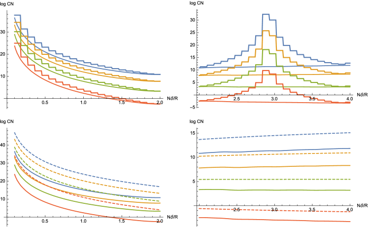
(a) $n=3,\;\eta=0.1,\;\mathcal{K}=3$

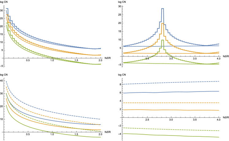
(b) $n=2,\;\eta=0.05,\;\mathcal{K}=3$

Figure 1: Estimating the condition numbers and their upper bounds. Upper row: decimated vs. non-decimated, super-resolution (upper left) and stable (upper right) regions. Lower row: undecimated condition numbers vs. upper bounds. CN stands for condition number ($\kappa$) and $\delta$ stands for $\eta$.

5.1.3 Conclusions

1. A “phase transition” between well-conditioned and ill-conditioned regions is seen to occur with the threshold in the range $\frac{N\eta}{R}\in\left(1,3\right)$.

2. In the “near ill-conditioned” (or “super-resolution”) region, the decimated condition number are almost identical with the non-decimated ones.

3. The computed upper bounds provide accurate growth rates in the region $N\eta\gg 1$, and are also relatively accurate in the super-resolution region.

4. The periodic pattern for $\kappa^{\left(p\right)}$ is seen in the well-conditioned region and it is well-predicted by the theory. For instance, it is easy to see that for infinite number of values of $p$ we have $\pi<p\eta^{*}<\pi+\varepsilon$ (recall Corollary 3.1), thus $\eta_{p}$ becomes small and $\kappa^{\left(p\right)}$ blows up.

5.2 Least Squares and ESPRIT with decimation

We have tested the decimation technique on two well-known algorithms for Prony systems - generalized ESPRIT [5] and nonlinear least squares (LS, implemented by MATLAB’s lsqnonlin). To avoid the aliasing problem, we assumed an initial approximation to be given. All computations were done in MATLAB with double precision floating point arithmetic. The computed values of $m_{k}$ were perturbed in a random manner with specified noise level.

In the first experiment, we fixed the number of measurements to be 66, and changed the decimation parameter $p$, while keeping the noise level constant. The accuracy of recovery increased with $p$ – see Figure 2 on page 2.

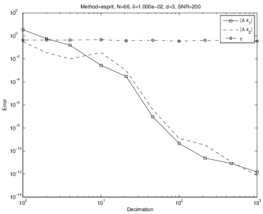
(a) ESPRIT, $\ell_{j}=3$

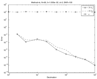
(b) LS, $\ell_{j}=3$

Figure 2: Reconstruction error as a function of the decimation with fixed number of measurements ($N=66$). The signal has two nodes with distance $\eta=10^{-2}$ between each other. Notice that ESPRIT requires significantly higher Signal-to-Noise Ratio in order to achieve the same performance as LS.

In the second experiment, we fixed the highest available measurement to be $N=1600$, and changed the decimation from $p=1$ to $p=100$ (thereby reducing the number of measurements from $1600$ to just $16$). The accuracy of recovery stayed relatively constant – see Figure 3 on page 3. Such a reduction leads to a corresponding decrease in the running time, since for instance the SVD computation in ESPRIT takes $O\left(N^{2}R\right)$.

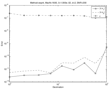
(a) ESPRIT, $\ell_{j}=2$

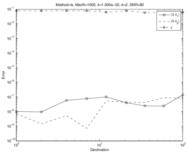
(b) LS, $\ell_{j}=2$

Figure 3: Reconstruction error as a function of the decimation, reducing number of measurements from $N=1600$ to $N=16$. The signal has two nodes with distance $\eta=10^{-2}$ between each other. The reconstruction accuracy remains almost constant.

6 Relation to existing work

Majority of the existing works in the literature consider the first order Prony system (2). Specializing the results of the present paper to this special case, we have the following result.

Theorem 6.6.

Consider the system (3) with $\ell_{1}=\dots=\ell_{\mathcal{K}}=1$, and with a-priori bounds as elaborated in Section 2.

1. For $N\eta\gg 1$ and for $j=1,\dots,\mathcal{K}$ we have (here $A=\sum_{m=1}^{\mathcal{K}}\left|a_{j}\right|$)

   $$\kappa_{2j-1,N} \lessapprox A,$$

   $$\kappa_{2j,N} \lessapprox \frac{A}{\left|a_{j}\right|}\cdot\frac{1}{N}.$$

2. If, on the other hand, all the nodes form a cluster, i.e. $N\eta^{*}<2\pi\mathcal{K}$, then

   $$\kappa_{2j-1}^{\left(p^{*}\right)} \lessapprox \frac{1}{\left(N\eta^{\left(j\right)}\right)^{2\mathcal{K}}},$$

   $$\kappa_{2j}^{\left(p^{*}\right)} \lessapprox \frac{1}{\left|a_{j}\right|}\cdot\frac{\eta^{\left(j\right)}}{\left(N\eta^{\left(j\right)}\right)^{2\mathcal{K}}}.$$

In his influential paper [23], Donoho gave bounds for noise amplification (modulus of continuity $\Lambda$) for recovery of signed measures from their continuous spectra of width $\Omega$ on a lattice with step size $\Delta$ in the superresolution setting $\Omega\Delta\ll\pi$. The ratio $\frac{1}{\Delta\Omega}$ is called the “super-resolution factor” (SRF). If the measure has at most $\ell$ nonzero coefficients, then $\Lambda$ is shown to increase at least as $\approx\left(\frac{1}{\Delta}\right)^{2\ell-1}$ and at most as $\approx\left(\frac{1}{\Delta}\right)^{2\ell+1}$. When $\Delta\to 0$, the lower bound effectively scales as $\left(SRF\right)^{2\ell-1}$, and the same scaling was recently shown to hold also for the upper bound by Demanet and Nguyen [21].

No practical way to achieve the above bounds have been proposed, however, recent works of Candes and Fernandez-Granda [17, 18, 29] showed that under an additional assumption of node separation (effectively putting $\ell=1$ above) a stable recovery via total variation (TV) minimization is possible, both for the $\ell_{1}$-norm and for the locations of the spikes. Additional recent works [25, 58] explore penalized TV approaches and provide similar stability estimates under various assumptions.

To express the above setting in the notations of this paper, we identify $\Delta$ with $\eta$, $\Omega$ with $N$ and $\ell$ with $\mathcal{K}$, and put $\ell_{j}=1$. After this identification, the second part of Theorem 6.6 gives an upper bound for the modulus of continuity of the order $\left(SRF\right)^{2\ell}$, which is slightly worse than the estimates in [21, 23]. Our setting is more general however, as the spikes are not assumed to lie on a grid. Furthermore, we also provide perturbation bounds for the locations of the spikes in terms of the super-resolution factor.

In a recent paper [43] the authors observed a phase transition for the (unstructured) condition number of Vandermonde matrices, a clear analogy with our results (note that in addition to a similar phase transition, our estimates also predict an exponential increase w.r.t $R$ in the condition number, see Subsection 4.1). In another related work, Demanet and Townsend [22] studied the problem of polynomial extrapolation of analytic functions, and they showed two different stability regimes, depending on the number of samples of the function – similar to what we have described in this paper. It would be highly interesting to relate these results to each other.

A method very similar to decimation, called “subspace shifting”, or interleaving, was proposed by Maravic & Vetterli in [42] in the context of analyzing performance of Finite Rate of Innovation (FRI) sampling in the presence of noise. Their idea was to interleave the rows of the Hankel matrix used in subspace estimation methods, effectively increasing the separation of closely spaced nodes. They confirmed this idea with numerical experiments. The results of our paper can be considered as a theoretical justification of their approach, and its extension to the more general system (3).

In statistical signal estimation, the Cramer-Rao Lower Bound (CRB) gives a lower bound for the variance of any unbiased estimator, see [37]). In [40] the authors only prove the CRB estimates for $\mathcal{K}=1,2$ and $N\gg 1$, for the system (2). On the other hand, the authors of [6] consider the more general system (3) (called PACE model), and derive asymptotic estimates for $N\gg 1$. These results are qualitatively similar to our Theorem 2.2 and Theorem 2.1. Obviously our results are different in nature from the CRB, but nevertheless the stated similarity is worth investigating further. Generalized ESPRIT is shown to asymptotically attain the CRB for $N\to\infty$.

The effect of oversampling for FRI signals was also studied in [16], where they showed that it can improve performance by several orders of magnitude - a conclusion which is certainly consistent with our Theorem 2.1.

Stability analysis of Approximate Prony method, carried out by the authors of [47, 48], suggests an increase in recovery error for the linear coefficients $a_{j}$, again consistent with our results (see [10] for further details).

Performance analysis of MUSIC in another recent paper [41] (see also a recent preprint [28] regarding ESPRIT) suggests that it can resolve arbitrarily close frequencies below $N^{-1}$ for sufficiently small noise - compare this with Theorem 2.1, which shows that the sensitivity indeed does not depend on the node separation.

The method of Filbir et. al [30] solves the system (2) via constructing a certain orthogonal polynomial on the unit circle. Their perturbation analysis gives an error in the nodes of the order of $\sqrt{\frac{\log N}{N}}$. Also, localized kernel methods were recently shown to provide stable estimation of instantaneous frequencies, under minimal separation assumption [19].

Decimation has recently appeared in zooming methods such as ZMUSIC [38] and zoom-ESPRIT [39] for reducing computational complexity and memory requirements for estimating frequencies in a specified range. Experiments show also improvement in accuracy of the zooming techniques w.r.t to their regular counterparts, thus it would be interesting to see whether an analysis similar to ours can be applied also in these cases.

A variant of decimation for Prony systems, called “arithmetic progression sampling” (APS) and described in detail in [54], was shown by Sidi to enhance substantially both the convergence acceleration and numerical stability properties of generalizations of the Richardson extrapolation process. It would be interesting to make this connection more elaborate and precise.

A kind of “stochastic decimation” (randomized arithmetic progression sampling) was recently used by Kaltofen et.al for outlier removal in sparse model synthesis and interpolation [36].

7 Some future directions

This paper is a part of a continuing research effort, investigating the applicability of algebraic methods to signal reconstruction problems [2, 7, 8, 9, 10, 12, 13, 14, 27, 51]. Some of its findings were initially reported in [11]. Building upon the presented ideas, we have recently proposed a novel “decimated homotopy” algorithm, which has been shown to achieve the accuracy specified in Corollary 3.1, and outperform state of the art methods such as ESPRIT in the near-colliding setting [7, 9]. Another extension of this work is reported in [2], providing tight global bounds (opposed to the first-order situation of this paper) for the accuracy of cluster recovery. Decimation also played a major role in our recent proposed algorithm for resolving the Gibbs phenomenon [8].

The numerical analysis of Prony systems in an important topic for further investigations. For instance, the bounds of Theorem 2.1 are valid for the noise model (8). However, in some applications such as [8], a more appropriate assumption is

$$\frac{\left|\Delta m_{k}\right|}{\left|m_{k}\right|}\leqslant\rho k^{-1},$$

for some fixed $\rho$. In general, “semi-global” analysis is required in this and similar settings, and we leave this for a future publication (cf. [2]).

An important open question connected with stable solution of Prony systems is how to detect the near-singular situations, and choose the problem structure vector $\boldsymbol{\ell}=\left(\ell_{1},\dots,\ell_{\mathcal{K}}\right)$ in an optimal way. One possible approach might involve symbolic-numeric techniques for polynomial systems, combined with analysis of the singularities of the mapping ${\cal P}_{N}$ ([12, 13]).

Under our assumption of a single cluster, decimation appears to provide near-optimal conditioning with respect to the number of samples $N$. While theoretical justification of this optimality would be desirable, a more important goal is to provide optimal solution when only some of the nodes form a cluster.

8 Acknowledgements

We would like to thank H. Mhaskar for useful suggestions regarding the manuscript.

References

References

- Abramowitz and Stegun [1965] M. Abramowitz and I. Stegun. Handbook of mathematical functions: with formulas, graphs, and mathematical tables. 1965.
- Akinshin et al. [2015] A. Akinshin, D. Batenkov, and Y. Yomdin. Accuracy of spike-train Fourier reconstruction for colliding nodes. In 2015 International Conference on Sampling Theory and Applications (SampTA), pages 617–621, May 2015. doi: 10.1109/SAMPTA.2015.7148965.
- Auton [1981] J. Auton. Investigation of Procedures for Automatic Resonance Extraction from Noisy Transient Electromagnetics Data. Volume III. Translation of Prony’s Original Paper and Bibliography of Prony’s Method. Technical report, Effects Technology Inc., Santa Barbara, CA, 1981.
- Azaïs et al. [2015] J.-M. Azaïs, Y. de Castro, and F. Gamboa. Spike detection from inaccurate samplings. Applied and Computational Harmonic Analysis, 38(2):177–195, Mar. 2015. ISSN 1063-5203. doi: 10.1016/j.acha.2014.03.004. URL http://www.sciencedirect.com/science/article/pii/S106352031400044X.
- Badeau et al. [2008a] R. Badeau, B. David, and G. Richard. Performance of ESPRIT for estimating mixtures of complex exponentials modulated by polynomials. IEEE Transactions on Signal Processing, 56(2):492–504, 2008a. ISSN 1053-587X.
- Badeau et al. [2008b] R. Badeau, B. David, and G. Richard. Cramér–Rao bounds for multiple poles and coefficients of quasi-polynomials in colored noise. IEEE Transactions on Signal Processing, 56(8):3458–3467, 2008b. ISSN 1053-587X.
- Batenkov [2014] D. Batenkov. Prony Systems via Decimation and Homotopy Continuation. In Proceedings of the 2014 Symposium on Symbolic-Numeric Computation, SNC ’14, page 59–60, New York, NY, USA, 2014. ACM. ISBN 978-1-4503-2963-7. doi: 10.1145/2631948.2631961. URL http://doi.acm.org/10.1145/2631948.2631961.
- Batenkov [2015] D. Batenkov. Complete algebraic reconstruction of piecewise-smooth functions from Fourier data. Mathematics of Computation, 84(295):2329–2350, 2015. ISSN 0025-5718, 1088-6842. doi: 10.1090/S0025-5718-2015-02948-2. URL http://www.ams.org/mcom/2015-84-295/S0025-5718-2015-02948-2/.
- Batenkov [2016] D. Batenkov. Accurate solution of near-colliding Prony systems via decimation and homotopy continuation. Accepted for publication in Theoretical Computer Science, 2016. URL http://arxiv.org/abs/1501.00160. arXiv: 1501.00160.
- Batenkov and Yomdin [2013a] D. Batenkov and Y. Yomdin. On the accuracy of solving confluent Prony systems. SIAM J. Appl. Math., 73(1):134–154, 2013a.
- Batenkov and Yomdin [2013b] D. Batenkov and Y. Yomdin. Algebraic signal sampling, Gibbs phenomenon and Prony-type systems. In Proceedings of the 10th International Conference on Sampling Theory and Applications (SAMPTA), 2013b.
- Batenkov and Yomdin [2014] D. Batenkov and Y. Yomdin. Geometry and Singularities of the Prony mapping. Journal of Singularities, 10:1–25, 2014. ISSN 19492006. doi: 10.5427/jsing.2014.10a. URL http://www.journalofsing.org/volume10/article1.html.
- Batenkov and Yomdin [2015] D. Batenkov and Y. Yomdin. Local and Global Geometry of Prony Systems and Fourier Reconstruction of Piecewise-Smooth Functions. In Operator-Related Function Theory and Time-Frequency Analysis, pages 57–76. Springer, 2015. URL http://link.springer.com/chapter/10.1007/978-3-319-08557-9_2.
- Batenkov et al. [2012] D. Batenkov, N. Sarig, and Y. Yomdin. An "algebraic" reconstruction of piecewise-smooth functions from integral measurements. Functional Differential Equations, 19(1-2):9–26, 2012.
- Beckermann et al. [2007] B. Beckermann, G. H. Golub, and G. Labahn. On the numerical condition of a generalized Hankel eigenvalue problem. Numerische Mathematik, 106(1):41–68, Mar. 2007. ISSN 0029-599X, 0945-3245. doi: 10.1007/s00211-006-0054-x. URL http://link.springer.com/article/10.1007/s00211-006-0054-x.
- Ben-Haim et al. [2012] Z. Ben-Haim, T. Michaeli, and Y. Eldar. Performance Bounds and Design Criteria for Estimating Finite Rate of Innovation Signals. IEEE Transactions on Information Theory, 58(8):4993–5015, 2012. ISSN 0018-9448. doi: 10.1109/TIT.2012.2197719.
- Candès and Fernandez-Granda [2013] E. J. Candès and C. Fernandez-Granda. Super-resolution from noisy data. Journal of Fourier Analysis and Applications, 19(6):1229–1254, Dec. 2013. ISSN 1069-5869, 1531-5851. doi: 10.1007/s00041-013-9292-3. URL http://link.springer.com/article/10.1007/s00041-013-9292-3.
- Candès and Fernandez-Granda [2014] E. J. Candès and C. Fernandez-Granda. Towards a mathematical theory of super-resolution. Communications on Pure and Applied Mathematics, 67(6):906–956, June 2014. ISSN 1097-0312. doi: 10.1002/cpa.21455. URL http://onlinelibrary.wiley.com/doi/10.1002/cpa.21455/abstract.
- Chui and Mhaskar [2016] C. K. Chui and H. N. Mhaskar. Signal decomposition and analysis via extraction of frequencies. Applied and Computational Harmonic Analysis, 40(1):97–136, Jan. 2016. ISSN 1063-5203. doi: 10.1016/j.acha.2015.01.003. URL http://www.sciencedirect.com/science/article/pii/S1063520315000044.
- Conway and Guy [1995] J. H. Conway and R. Guy. The Book of Numbers. Copernicus, New York, NY, corrected edition, Mar. 1995. ISBN 978-0-387-97993-9.
- Demanet and Nguyen [2014] L. Demanet and N. Nguyen. The recoverability limit for superresolution via sparsity. Preprint, 2014. URL http://math.mit.edu/icg/papers/scaling-superres.pdf.
- Demanet and Townsend [2016] L. Demanet and A. Townsend. Stable extrapolation of analytic functions. arXiv:1605.09601 [cs, math], May 2016. URL http://arxiv.org/abs/1605.09601. arXiv: 1605.09601.
- Donoho [1992] D. Donoho. Superresolution via sparsity constraints. SIAM Journal on Mathematical Analysis, 23(5):1309–1331, 1992.
- Dragotti et al. [2007] P. L. Dragotti, M. Vetterli, and T. Blu. Sampling moments and reconstructing signals of finite rate of innovation: Shannon meets strang-fix. IEEE Transactions on Signal Processing, 55(5):1741, 2007.
- Duval and Peyré [2014] V. Duval and G. Peyré. Exact Support Recovery for Sparse Spikes Deconvolution. Foundations of Computational Mathematics, 15(5):1315–1355, Oct. 2014. ISSN 1615-3375, 1615-3383. doi: 10.1007/s10208-014-9228-6. URL http://link.springer.com/article/10.1007/s10208-014-9228-6.
- Elad et al. [2004] M. Elad, P. Milanfar, and G. H. Golub. Shape from moments-an estimation theory perspective. Signal Processing, IEEE Transactions on, 52(7):1814–1829, 2004. URL http://ieeexplore.ieee.org/xpls/abs_all.jsp?arnumber=1306639.
- Ettinger et al. [2008] B. Ettinger, N. Sarig, and Y. Yomdin. Linear versus Non-Linear Acquisition of Step-Functions. Journal of Geometric Analysis, 18(2):369–399, Apr. 2008. ISSN 1050-6926, 1559-002X. doi: 10.1007/s12220-008-9016-0. URL http://link.springer.com/article/10.1007/s12220-008-9016-0.
- Fannjiang [2016] A. Fannjiang. Compressive Spectral Estimation with Single-Snapshot ESPRIT: Stability and Resolution. arXiv:1607.01827 [cs, math], July 2016. URL http://arxiv.org/abs/1607.01827. arXiv: 1607.01827.
- Fernandez-Granda [2013] C. Fernandez-Granda. Support detection in super-resolution. In Proc. of 10th Sampling Theory and Applications (SAMPTA), pages 145—148, 2013. URL http://arxiv.org/abs/1302.3921.
- Filbir et al. [2012] F. Filbir, H. N. Mhaskar, and J. Prestin. On the problem of parameter estimation in exponential sums. Constructive Approximation, 35(3):323–343, 2012. URL http://link.springer.com/article/10.1007/s00365-011-9136-9.
- Gautschi [1962] W. Gautschi. On inverses of Vandermonde and confluent Vandermonde matrices. Numerische Mathematik, 4(1):117–123, 1962.
- Gautschi [1963] W. Gautschi. On inverses of Vandermonde and confluent Vandermonde matrices. II. Numerische Mathematik, 5(1):425–430, 1963.
- Golub et al. [2000] G. H. Golub, P. Milanfar, and J. Varah. A Stable Numerical Method for Inverting Shape from Moments. SIAM Journal on Scientific Computing, 21(4):1222–1243, 2000.
- Gustafsson et al. [2000] B. Gustafsson, C. He, P. Milanfar, and M. Putinar. Reconstructing planar domains from their moments. Inverse Problems, 16(4):1053–1070, 2000.
- Higham [1994] N. J. Higham. A survey of componentwise perturbation theory in numerical linear algebra. In Proceedings of symposia in applied mathematics, volume 48, page 49–77, 1994. URL http://www.google.com/books?hl=en&lr=&id=vSdUw1HRuwMC&oi=fnd&pg=PA49&ots=fX4VcPcBFd&sig=TkuOxpYvZikq8QSnSIFU-_0ztag.
- Kaltofen [2014] E. L. Kaltofen. Cleaning-up data for sparse model synthesis: When symbolic-numeric computation meets error-correcting codes. In Proceedings of the 2014 Symposium on Symbolic-Numeric Computation, SNC ’14, pages 1–2, New York, NY, USA, 2014. ACM. ISBN 978-1-4503-2963-7. doi: 10.1145/2631948.2631949. URL http://doi.acm.org/10.1145/2631948.2631949.
- Kay [1993] S. Kay. Fundamentals of Statistical Signal Processing. Prentice-Hall, 1993.
- Kia et al. [2007] S. Kia, H. Henao, and G.-A. Capolino. A High-Resolution Frequency Estimation Method for Three-Phase Induction Machine Fault Detection. IEEE Transactions on Industrial Electronics, 54(4):2305–2314, Aug. 2007. ISSN 0278-0046. doi: 10.1109/TIE.2007.899826.
- Kim et al. [2013] Y.-H. Kim, Y.-W. Youn, D.-H. Hwang, J.-H. Sun, and D.-S. Kang. High-Resolution Parameter Estimation Method to Identify Broken Rotor Bar Faults in Induction Motors. IEEE Transactions on Industrial Electronics, 60(9):4103–4117, Sept. 2013. ISSN 0278-0046. doi: 10.1109/TIE.2012.2227912.
- Kusuma and Goyal [2009] J. Kusuma and V. K. Goyal. On the accuracy and resolution of powersum-based sampling methods. IEEE Transactions on Signal Processing, 57(1):182–193, 2009.
- Liao and Fannjiang [2016] W. Liao and A. Fannjiang. MUSIC for single-snapshot spectral estimation: Stability and super-resolution. Applied and Computational Harmonic Analysis, 40(1):33–67, Jan. 2016. ISSN 1063-5203. doi: 10.1016/j.acha.2014.12.003. URL http://www.sciencedirect.com/science/article/pii/S1063520314001432.
- Maravic and Vetterli [2005] I. Maravic and M. Vetterli. Sampling and reconstruction of signals with finite rate of innovation in the presence of noise. IEEE Transactions on Signal Processing, 53(8 Part 1):2788–2805, 2005.
- Moitra [2015] A. Moitra. Super-resolution, Extremal Functions and the Condition Number of Vandermonde Matrices. In Proceedings of the Forty-Seventh Annual ACM on Symposium on Theory of Computing, STOC ’15, pages 821–830, New York, NY, USA, 2015. ACM. ISBN 978-1-4503-3536-2. doi: 10.1145/2746539.2746561. URL http://doi.acm.org/10.1145/2746539.2746561.
- O’Leary and Rust [2013] D. P. O’Leary and B. W. Rust. Variable projection for nonlinear least squares problems. Computational Optimization and Applications, 54(3):579–593, 2013. URL http://link.springer.com/article/10.1007/s10589-012-9492-9.
- Pereyra and Scherer [2010] V. Pereyra and G. Scherer. Exponential Data Fitting and Its Applications. Bentham Science Publishers, Jan. 2010. ISBN 9781608050482.
- Peter and Plonka [2013] T. Peter and G. Plonka. A generalized Prony method for reconstruction of sparse sums of eigenfunctions of linear operators. Inverse Problems, 29(2):025001, Feb. 2013. ISSN 0266-5611. doi: 10.1088/0266-5611/29/2/025001. URL http://iopscience.iop.org/0266-5611/29/2/025001.
- Peter et al. [2011] T. Peter, D. Potts, and M. Tasche. Nonlinear approximation by sums of exponentials and translates. SIAM Journal on Scientific Computing, 33(4):1920, 2011.
- Potts and Tasche [2010] D. Potts and M. Tasche. Parameter estimation for exponential sums by approximate Prony method. Signal Processing, 90(5):1631–1642, 2010.
- Prony [1795] R. Prony. Essai experimental et analytique. J. Ec. Polytech.(Paris), 2:24–76, 1795.
- Rao and Arun [1992] B. D. Rao and K. S. Arun. Model based processing of signals: A state space approach. Proceedings of the IEEE, 80(2):283–309, 1992.
- Sarig and Yomdin [2008] N. Sarig and Y. Yomdin. Signal Acquisition from Measurements via Non-Linear Models. Mathematical Reports of the Academy of Science of the Royal Society of Canada, 29(4):97–114, 2008.
- Schappelle [1972] R. Schappelle. The inverse of the confluent Vandermonde matrix. IEEE Transactions on Automatic Control, 17(5):724–725, 1972.
- Sidi [1982] A. Sidi. Interpolation at equidistant points by a sum of exponential functions. Journal of Approximation Theory, 34(2):194–210, 1982. URL http://www.sciencedirect.com/science/article/pii/0021904582900922.
- Sidi [2003] A. Sidi. Practical extrapolation methods: Theory and applications. Cambridge University Press, 2003.
- Spitzbart [1960] A. Spitzbart. A generalization of Hermite’s interpolation formula. American Mathematical Monthly, pages 42–46, 1960.
- Stetter [2004] H. J. Stetter. Numerical polynomial algebra. SIAM, 2004. URL http://www.google.com/books?hl=en&lr=&id=bnBrsj_cA2gC&oi=fnd&pg=PR2&dq=stetter+numerical+polynomial+algebra&ots=QHVMS_N6TA&sig=0o-YZNlg4JPRU-W7Jsub5sBFmTs.
- Stoica and Moses [2005] P. Stoica and R. Moses. Spectral analysis of signals. Pearson/Prentice Hall, 2005.
- Tang et al. [2015] G. Tang, B. N. Bhaskar, and B. Recht. Near Minimax Line Spectral Estimation. IEEE Transactions on Information Theory, 61(1):499–512, Jan. 2015. ISSN 0018-9448. doi: 10.1109/TIT.2014.2368122.
- Van Blaricum and Mittra [1978] M. L. Van Blaricum and R. Mittra. Problems and solutions associated with Prony’s method for processing transient data. IEEE Transactions on Antennas and Propagation, AP-26(1):174–182, 1978.