Abstract

pde2path 2.0 is an upgrade of the continuation/bifurcation package pde2path for elliptic systems of PDEs over bounded 2D domains, based on Matlab’s pdetoolbox. The new features include a more efficient use of FEM, easier switching between different single parameter continuations, genuine multi–parameter continuation (e.g., fold continuation), more efficient implementation of nonlinear boundary conditions, cylinder and torus geometries (i.e., periodic boundary conditions), and a general interface for adding auxiliary equations like mass conservation or phase equations for continuation of traveling waves. The package (library, demos, manuals) can be downloaded at www.staff.uni-oldenburg.de/hannes.uecker/pde2path.

MSC: 35J47, 35J60, 35B22, 65N30
Keywords: elliptic systems, continuation and bifurcation, finite element method

1 Introduction

pde2path, based on the FEM of the Matlab pdetoolbox, is a continuation/bifurcation package for elliptic systems of PDEs of the form

$$G(u,\lambda):=-\nabla\cdot(c\otimes\nabla u)+au-b\otimes\nabla u-f=0,$$ (1)

where $u=u(x)\in{\mathbb{R}}^{N}$, $x\in\Omega\subset{\mathbb{R}}^{2}$ some bounded domain, $\lambda\in{\mathbb{R}}^{p}$ is a parameter (vector), $c\in{\mathbb{R}}^{N\times N\times 2\times 2}$, $b\in{\mathbb{R}}^{N\times N\times 2}$, $a\in{\mathbb{R}}^{N\times N}$ and $f\in{\mathbb{R}}^{N}$ can depend on $x,u,\nabla u$, and, of course, parameters. The boundary conditions (BC) are “generalized Neumann” of the form

$${\bf n}\cdot(c\otimes\nabla u)+qu=g,$$ (2)

where ${\bf n}$ is the outer normal and again $q\in{\mathbb{R}}^{N\times N}$ and $g\in{\mathbb{R}}^{N}$ may depend on $x$, $u$ and parameters. These BC include prescribed flux BC, and a “stiff spring” approximation of Dirichlet BC via large prefactors in $q$ and $g$.

For the basic ideas of continuation/bifurcation, the algorithms, and the class of systems we aim at, i.e., the meaning of the terms in (1) and the associated boundary conditions, we refer to [13], and the references therein. Here we explain a number of additional features in pde2path 2.0, in short p2p2, compared to the version documented in [13], and some changes in the underlying data structures. The new features include:

1. easy switching between different single parameter continuations;

2. genuine multi–parameter continuation, in particular automatic fold and branch point continuation;

3. general interface for adding auxiliary equations, such as mass conservation, or freezing-type equations for continuation of traveling waves;

4. periodic domains: cylinder and torus geometries;

5. fast FEM for a subclass of (1), roughly where $c,a,b,q$ and $g$ are independent of $u$, i.e., where nonlinearity enters only through $f$;

6. improved and more user-friendly plotting.

We explain these features by a number of examples, but first describe the major structural changes (items 1,2,3).

Remark 1.1.

The concept of p2p2 is that of a box of customizable tools. These tools (functions) are in p2p2/p2plib, which must be in the Matlab path. When starting Matlab in the p2p2 home directory, execute setpde2path. The demo directories are under p2p2/demos/. Each demo (with name *) comes with one or more script-files *cmds.m, which typically are organized in cells, i.e., should be stepped through cell by cell. To get help on any p2p2 function, e.g., cont, type help cont or doc cont. To get started type help p2phelp. Additional Matlab–internal and online html–help will be added shortly.

To set up a new problem in p2p2 we recommend to copy a suitable demo directory (i.e., a demo directory which considers a similar problem) to a new working directory and start modifying the pertinent files. To customize any of the functions from p2p2/p2plib we recommend to copy it to the working directory and modify it there (thus “overloading” the file from p2p2/p2lib). $\rfloor$

Remark 1.2.

The new data structure and different user interfaces mean that there is no downward compatibility with [13]. On the other hand, we think that upgrading old pde2path files to p2p2 is quickly achieved, and that the data structure and user interfaces now have a final form. $\rfloor$

Parameters, auxiliary variables and auxiliary equations.

A p2p2 problem is described by a matlab structure p. The most drastic change compared to [13] is that no single distinguished parameter $\lambda$ appears in p anymore, but any number of auxiliary variables, typically parameters, can be added. If the FEM mesh has $n_{p}=$np points and $N=$neq in (1) we have $n_{u}=Nn_{p}=$p.nu=neq*p.np unknown nodal values for $u$, (except in the case of periodic BC, see below), and p.u(1:p.nu) contains these nodal values.

The arbitrary number of auxiliary variables are stored in p.u(p.nu+1:end) and can be “passive”, serving as constant parameters, or “active” unknowns to be solved for. In the following we write, on the discrete level, $U=(u,w)=$p.u, where $u$ corresponds to (the nodal values of) the PDE variables in (1) and $w$ the auxiliary variables. Suppose there are $n_{q}+1$ active variables $w_{{\rm act}}\in{\mathbb{R}}^{n_{q}+1}$. Exactly one of these is the “primary” active parameter, and we write $w_{{\rm act}}=(\tilde{w},\alpha)$. The remaining $n_{q}$ active variables require $n_{q}$ additional (‘auxiliary’) equations

$$q_{i}(U)=0,\quad i=1,\ldots,n_{q}.$$ (3)

In the functions defining $G$ or its Jacobian a typical first step is to split off the PDE part $u$ as shown in the examples below. The active auxiliary variables are selected by the user in the array of indices p.nc.ilam, whose first entry is the primary continuation parameter. For different continuation tasks the user may freely modify this list to choose different active, passive and primary parameters. Thus, $w_{{\rm act}}=(\tilde{w},\alpha)$ is only a symbolic notation, and the role of parameters (primary, active, passive) is determined by p.nc.ilam. For convenience, the routines printaux and getaux can be used to obtain all or only the active auxiliary variables. Internally, the routines au2u and u2au are used to transform p.u into the vector suitable for the Newton-loop or back to the full p.u.

Examples of additional equations are

• prescribed mass: $\int u\,{\rm d}x-m=0$, $m\in{\mathbb{R}}$, see, e.g., §2.4;

• a phase condition $\langle\partial_{x}u,u-u_{\rm old}\rangle_{2}=0$ for the continuation of traveling waves, see, e.g., §2.5.

As discussed in [13], it is useful to give $u$ and the continuation parameter different weights in the arclength equation

$$p(U,s)=\left\langle\dot{U},U(s)-U_{0}\right\rangle-(s-s_{0})=0;$$ (4)

see [13, §2.1]. In p2p2  this is extended to the active variables in $w_{{\rm act}}=(\tilde{w},\alpha)$, and as scalar product in (4) we use,

$$\left\langle(u,\tilde{w},\alpha),(v,\tilde{z},\beta)\right\rangle:=\xi\left\langle u,v\right\rangle_{2}+\xi_{q}\left\langle\tilde{w},\tilde{z}\right\rangle_{2}+(1-(\xi+\xi_{q})/2)\alpha\beta,$$ (5)

with independent weights $\xi$ and $\xi_{q}$ and $\left\langle\cdot,\cdot\right\rangle_{2}$ the euclidean inner product.

Numerical approximation of $\partial_{\lambda}G$.

In order to ease switching between different primary parameters, and since finite difference approximations of derivatives of $G$ with respect to just one parameter are relatively cheap, we deleted all explicit references to $\partial_{\lambda}G$. Hence, the interfaces for the functions defining $G(u)$ and its Jacobian now read function [c,a,f,b]=G(p,u) and function [cj,aj,bj]=Gjac(p,u), see the examples below.

Substructures of p: Names of numerical variables, switches, etc.

In p2p2 the many switches and settings in the problem structure variable p in [13] are now grouped as explained in Table LABEL:tab1a, i.e., function handles are entries in p.fuha, numerical controls are entries in p.nc, and so on. See also Appendix A. In particular, this makes it easier to get an overview over current parameter settings. For instance, to see the values of (all) the numerical control parameters for a given p, type p.nc on the command line. Of course, the user is free to add as many additional fields/variables to the structure p as desired/needed. If there are many of these, then we recommend to organize them in a substructure p.usr, say.

An example of a (here predefined) “user”–field is p.usrlam, which may contain target values for the primary parameter $\lambda$. This means that if during continuation u(p.nu+p.nc.ilam(1)) passes a value $\lambda^{*}$ in [p.usrlam,p.nc.lammin,p.nc.lammax], then the algorithm calculates and saves to file the solution at $\lambda^{*}$. The names of files containing solution data at a continuation point have changed from the previous (p.dir/)p*.mat to (p.dir/)pt*.mat. Similarly, the solution at a bifurcation point is saved in bpt*.mat and a fold point is saved in fpt*.mat.

Table 1: Fields in structure p; see stanparam.m in p2plib for detailed information on the contents of these fields and the standard settings, and the reference card in Appendix A.

field	purpose	field	purpose
fuha	function handles, e.g., fuha.G, …	nc	numerical controls, e.g., nc.tol, …
sw	switches such as sw.bifcheck,…	sol	values/fields calculated at runtime
eqn	tensors $c,a,b$ for fast FEM setup	mesh	the geometry data and mesh
plot	switches and controls for plotting	file	switches etc for file output
time	timing information	pm	pmcont switches
fsol	switches for the fsolve interface	nu,np	# PDE unknowns, # meshpoints
u,tau	solution and tangent	branch	branch data
usrlam	vector of user set target values for the primary parameter, default usrlam=[];
mat	problem matrices, in general data that is not saved to file, see Remark 2.3

Further general comments.

Concerning the improved plotting, p2p2  uses telling axis labelling and, for instance, a simplified user-friendly branch-plotting command: plotbra(p). By default, this plots the branch with primary parameter on the $x$-axis and $L^{2}$-norm (now stored in the internal part of the branch data) on the $y$-axis; the figure used can be controlled by p.plot.brafig. Similarly, plotbraf(’p’) is now allowed for convenience and calls plotbra(p) with structure p from the file in directory ’p’ with the highest point label. Moreover, in demo schnakfold we provide some examples how to create movies of some continuation.

Finally, we also added a wrapper to call Matlab’s fsolve routine; allthough this is typically slower than our own Newton loops, it may be useful, for instance, to find solutions from poor initial guesses, see §2.4.

Acknowledgement

We thank Ben Schweizer (TU Dortmund) for help on the transformation to periodic boundary conditions used in §2.6.

2 New features - by examples

2.1 Allen-Cahn model (acfold)

As a first example we (re)consider the cubic–quintic Allen-Cahn equation from [13, §3.2], written as

$$-c\Delta u-\lambda u-u^{3}+\gamma u^{5}=0,$$ (6)

on the rectangle $\Omega=(-1,1)\times(-0.9,0.9)$ with homogeneous Dirichlet BC. Our first task is to explain the new meaning of p.u, parameter–switching and fold–continuation, and a new setup with a more efficient use of the FEM. The demo directory for this is acfold.

2.1.1 Parameter switching

There are three parameters $c,\lambda,\gamma$, and in addition to the standard domain and BC setup known from [13], the init-routine acfold$\_$init now initializes these and sets the primary continuation parameter:

% initialize auxiliary variables, here parameters of PDE
par(1)=1;         % linear cofficient of f
par(2)=0.25;      % diffusion coefficient
par(3)=1;         % quintic coefficient of f
p.u=[p.u; par’];  % augment p.u by parameters
p.nc.ilam=1;      % set active parameter indices (here only one)
p.usrlam=[3.5 4]; % "target" values of the parameter

The functions defining $G$ and its Jacobian read

function [c,a,f,b]=acfold_G(p,u)  % coefficient functions for AC
% separate pde and auxiliary variables, here "par", and interpolate to triangles
par=u(p.nu+1:end); u=pdeintrp(p.points,p.tria,u(1:p.nu));
c=par(2); a=0; b=0; f=par(1)*u+u.^3-par(3)*u.^5; end;

function [cj,aj,bj]=acfold_Gjac(p,u)  % jacobian for AC
par=u(p.nu+1:end); u=pdeintrp(p.points,p.tria,u(1:p.nu));
cj=par(2); bj=0; fu=par(1)+3*u.^2-par(3)*5*u.^4;  aj=-fu; end

Remark 2.1.

We recall, see [13, Remark 3.2], that cj,aj,bj in Gjac are not the derivatives of $c,a,b$ in $G$. The notation only indicates that cj,aj,bj are the coefficients needed to assemble $G_{u}$. In general, the relation between cj,aj,bj and $c,a,b,f$ can be quite complicated, and only if $c,a,b$ are independent of $u$, and $f$ only depends on $u$ without derivatives (roughly: the semilinear case), then cj$=c$, bj$=b$, and aj$=a-f_{u}$. Similar remarks apply to the functions p.fuha.bc and p.fuha.bcjac, see §2.3. $\rfloor$

2.1.2 Efficient use of FEM matrices in the semilinear case

Exploiting a semilinear structure in the FEM assembling can give a significant computational speedup: the FEM representation $G(u)=Ku-F$ of, e.g., $-\Delta u-f(u)$, can be obtained directly from $Ku$=p.mat.K*u and $F=$p.mat.M*f(u), where p.mat.M and p.mat.K are the pre-assembled mass and stiffness matrices, and f(u) denotes $f(u)$ as nodal values. In contrast, the FEM assembling via the general routine [c,a,f,b]=G(p,u), calculates the coefficients c,a,f,b on the triangles after interpolation, and then K, F are assembled from these at every Newton step.

In p2p2  the faster FEM setting is turned on by p.eqn.sfem=1, which requires implementing the nodal routines for the Jacobian and residual, as well as setting the divergence tensor and, if needed, the advection tensor. The matrices $M$ and $K$ are then generated via p=setfemops(p) and stored in the structure p.mat. For the acfold demo the setup in acfold$\_$init reads
p.sw.sfem=1; p.fuha.sG=@acfold$\_$sG; p.fuha.sGjac=@acfold$\_$sGjac;
p.eqn.c=1; p.eqn.b=0; p.eqn.a=0;
and the relevant routines are:

function r=acfold_sG(p,u)
par=u(p.nu+1:end); u=u(1:p.nu); f=par(1)*u+u.^3-par(3)*u.^5;
r=par(2)*p.mat.K*u(1:p.nu)-p.mat.M*f; end

function Gu=acfold_sGjac(p,u)
par=u(p.nu+1:end); fu=par(1)+3*u.^2-par(3)*5*u.^4; Fu=spdiags(fu,0,p.nu,p.nu);
Gu=par(2)*p.mat.K-p.mat.M*Fu; end

For problems involving the advection tensor $b$, analogously define p.eqn.b and use the matrix p.mat.Kadv in the routines; see the acfront and acffold demos and, for a system, the schnaktravel and nlb demos. Assembling the mass matrix at startup, and automatic updates at mesh adaption or refinement, are controlled by setting p.sw.sfem to a nonzero value. If the user only wants to use pre-assembled mass matrix (hence no fast FEM for (1)), this would be p.sw.sfem=-1.

Remark 2.2.

(Customisation) If the operators in (1) depend on parameters, the “semilinear” implementation explained above can sometimes be extended by splitting the operators suitably. For instance, if the operator $c$ can be written as $c=c_{1}+\lambda c_{2}$, the routine setfemops can be locally (in the demo directory) modified to generate p.mat.K and p.mat.K2 so that the residual reads p.mat.K+lam*p.mat.K2. See §2.7.1 for an example. $\rfloor$

Remark 2.3.

(Mesh refinement, saving of FEM matrices) If a (semilinear) problem is to be run on a fixed mesh, then setting p.sw.sfem=1 and setting p.fuha.sG and p.fuha.sjac as above can replace the old setting with p.fuha.G completely. However, if adaptive mesh refinement is desired, then p.fuha.G is still needed to identify the triangles to be refined. The required new matrices p.mat.M, p.mat.K and p.mat.Kadv are automatically reassembled during mesh adaption. Moreover, to save hard disk space, in the standard setting p.fuha.savefu=@standsavefu, the struct p.mat is not saved in the solution files. When loading via loadp, it is automatically regenerated. However, when loading a p struct into the Matlab  workspace by a double click, this is not the case and a manual call to setfemops is needed. $\rfloor$

Remark 2.4.

(time integration) Although p2p2 is not primarily intended for time integration, we also provide some extensions of the simple general time–integrator tint from [13] for systems ${\partial}_{t}u=-G(u,\lambda)$. tintx uses the same (linearly implicit) algorithm as tint, based on the full p.fuha.G syntax, but also returns a time–series of the residual at each plotting step, and saves the time evolution in p.file.pre. In detail, at startup, the full structure p is saved (if it does not yet exist) to “pre/pt0.mat”, and afterwards only p.u is saved at the selected time steps. To load a point ptn from “pre”, we then use a modified p=loadp2(pre,’ptn’,’pt0’).

For the fast FEM setting sfem=1 the integrators tints and tintxs are much more efficient – typically by at least a factor 10. Again these are simple linearly implicit schemes, but based on an LU decompostion of $M+dtK$. See §2.2.2 for more comments. $\rfloor$

2.1.3 Fold detection, point types and parameter switching

Coming back to (6), after locating the well-known bifurcation points (eigenvalues of the Dirichlet Laplacian) from the trivial branch $u\equiv 0$, we switch in acfold$\_$cmds to the first bifurcating branch and continue it including fold-detection by

q=swibra(’p’,’bpt1’,’q’,-0.2); q.sw.foldcheck=1; p=cont(p);

where fold detection works by bisection as for branch points. The resulting branch is plotted in Figure 1(a) with the fold point marked. It is also stored in the file q/fpt1.mat and assigned a special point type in the branch p.branch. These point types in p2p2  branches are:

-1	= initial point or restart
-2	= guess from swibra for the initialization of branch switching
0	= regular point
1	= bifurcation point (found with bifdetec)
2	= fold point (found with folddetec)

(a)	(b)	(c)	(d)

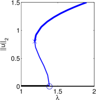
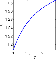
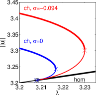
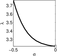
Figure 1: Fold continuation in the Allen–Cahn model (6) and the Schnakenberg model (9). (a),(b) First bifurcating branch ($(c,\gamma)=(0.25,1)$) and “fold position” $\lambda$ over the quintic parameter $\gamma$ in (6). (c) “cold hexagon” solution branch (blue) for (9) with $\sigma{=}0$. (d) continuation of the fold for $\sigma{=}0$ from (c) in $\sigma$; afterwards, the red branch in (c) was obtained via foldexit at $\sigma\approx-0.094$ and continuing in $\lambda$ again, with positive and negative ds. For details see acfold_cmds.m and schnakcmds.m, respectively.

Switching parameters in order to continue a stored solution in the previously constant diffusion rate $c$ (parameter number 2 in the implementation) goes simply by w=swiparf(’q’,’pt10’,’w’,2); where the essential change done by swiparf is setting w.ilam=2 and where w is the name of the new branch and q/pt10 is the file name of the stored solution. Before continuation by w=cont(w); some adjustments to the settings are useful in this case:

w.nc.lammin=0.1; w.sol.ds=-0.01; w.sol.xi=1e-6;

where the small weight $\xi$ is useful since the problem is more sensitive in the diffusion coefficient.

2.1.4 Fold and branch point continuation

We explain continuation of the fold-point in the q–branch in Fig. 1(a). Constraining continuation to folds requires an additional free parameter, e.g, $w:=(\lambda,\gamma)$. Before going into the practice in p2p2 we briefly discuss the background of fold–(and branchpoint–) continuation. In this case p2p2 discretizes the extended system

$$H(U)=\begin{pmatrix}G(u,w)\\ \partial_{u}G(u,w)\phi\\ \|\phi\|^{2}_{L^{2}}-1\\ p(U)\end{pmatrix}=0,\quad U=(u,\phi,w),$$ (7)

so that $\phi$ is in the kernel of $\partial_{u}G$ with $L^{2}$-norm constrained to 1 by the third equation, and $p(U)=0$ is the arclength equation (4). Thus the FEM discretization of (7) is a system of p.nu+p.nu+2 equations in p.nu+p.nu+1 unknowns.

For continuation of (7) we need the Jacobian

$$D_{U}H(U)=\begin{pmatrix}{\partial}_{u}G&0&{\partial}_{w}G\\ {\partial}_{u}({\partial}_{u}G\phi)&{\partial}_{u}G&{\partial}_{w}({\partial}_{u}G\phi)\\ 0&2\phi^{T}&0\\ \xi\dot{u}^{T}&\xi\dot{\phi}^{T}&(1-(\xi+\xi_{q})/2)\dot{w}\end{pmatrix},$$ (8)

where depending on p.sw.jac and p.sw.sfem ${\partial}_{u}G$ is calculated numerically or assembled using p.fuha.Gjac or p.fuha.Gjac, respectively, $\phi$ only occurs linearly in (7), derivatives with respect to $w$ are done via finite differences, and the computationally most costly part is the evaluation of ${\partial}_{u}({\partial}_{u}G\phi)$. While this is done numerically for p.sw.spjac=0, the user is urged to implement ${\partial}_{u}({\partial}_{u}G\phi)$ in a routine p.fuha.spjac and set p.sw.spjac=1.

In the acfold demo, this is readily done since ${\partial}_{u}({\partial}_{u}G\phi)=f_{uu}\phi$ so that we can use a pre-assembled mass matrix p.mat.M as in the FEM assembling for semilinear problems discussed in §2.1.2:

function Guuph=acfold_spjac(p,u)
ph=u(p.nu+1:2*p.nu); par=u(2*p.nu+1:length(u)); u=u(1:p.nu);
fuu=6*u-20*par(3)*u.^3; Guuph=-(p.mat.M*diag(fuu))*diag(ph);

The use of the extended system (7) and its Jacobian for subsequent continuations (the fold-/branch point-continuation mode) in p2p2  is turned on by calling spcontini; for instance (see acfold$\_$cmds):

qf=spcontini(’q’,’fpt1’,3,’qf’);% init fold continuation with par 3 as new active parameter
qf.plot.bpcmp=3; clf(2);        % use this new parameter for plotting
qf.nc.tol=1e-5;                 % increase tolerance as typically required for fold cont.
qf.sol.ds=1e-3;                 % new stepsize in new primary parameter

The branch computed now by qf=cont(qf) is plotted in Fig. 1(a). Note here p.nc.ilam=[1;3]. Starting a normal continuation from a point stored during a fold- or branch point-continuation is done on by calling spcontexit as in:

q1=spcontexit(’qf’,’pt10’,’q1’); q1.nc.tol=1e-8; q1.sol.ds=1e-3; q1=cont(q1);

Remark 2.5.

The switch sw.spcont is internally used to distinguish these modes: 0 means normal, 1 means branch point and 2 means fold point continuation, in agreement with the point types mentioned above. This stores the continuation mode since during continuation of fold/branch points the point types are normally zero as for usual continuation. For branch switching from a branch point continuation it can be useful to generate a new guess for the tangent vector tau. This can be conveniently done with the new routine p=getinitau(p) and the new method to call swibra as in q=swibra(p,0.05,’q’). See the demo bratu for an example. $\rfloor$

2.2 Semilinear structure in a system: the Schnakenberg model (schnackfold)

2.2.1 Fold continuation

As an example of a system (i.e. $N=$neq$>1$) we consider the Schakenberg model

$${\partial}_{t}U=D\Delta U+N(u,\lambda)+\sigma\left(u-\frac{1}{v}\right)^{2}\begin{pmatrix}1\\ -1\end{pmatrix},\quad N(U,\lambda)=\begin{pmatrix}-u+u^{2}v\\ \lambda-u^{2}v\end{pmatrix},$$ (9)

with $U=(u,v)(t,x,y)\in{\mathbb{R}}^{2}$, diffusion matrix $D=\bigl{(}\begin{smallmatrix}1&0\\ 0&d\end{smallmatrix}\bigr{)}$, $d$ fixed to $d=60$, and bifurcation parameters $\lambda\in{\mathbb{R}}_{+}$ and $\sigma\in{\mathbb{R}}$. System (9) has the homogeneous stationary solution $(u,v)=(\lambda,1/\lambda)$, which becomes Turing unstable for $\lambda\leq\lambda_{c}\approx 3.2085$, independent of $\sigma$, with critical wave-vectors $k=(k_{1},k_{2},k_{3})$ with $|k|=k_{c}=\sqrt{\sqrt{2}{-}1}{\approx}0.6436$. Here $\sigma$ can be used to turn certain 2D bifurcations from sub–to supercritical, and many branches of patterns exhibit one or many folds (“snaking”) [13, §4.2] and [11]. Fold continuation can be used to discuss snaking widths, see [12], which however, requires rather large systems with grid size ${\cal O}(10^{5})$ so that finite differences for ${\partial}_{u}({\partial}_{u}G\phi)$ in (8) are inefficient.

Following the approach discussed in §2.1.2 for semilinear problems, here we implement ${\partial}_{u}({\partial}_{u}G\phi)$ in the simplified nodal FEM format (in the demo schnakfold also the PDE itself is implemented according to §2.1.2). Denoting $u=(u_{1},u_{2})$, $\phi=(\phi_{1},\phi_{2})$, $f=(f_{1},f_{2})$ for the components of $u,\phi$ and $f$, we have

$${\partial}_{u}({\partial}_{u}G\phi)=\begin{pmatrix}({\partial}_{u_{1}}^{2}f_{1})\phi_{1}+({\partial}_{u_{1}}{\partial}_{u_{2}}f_{1})\phi_{2}&({\partial}_{u_{1}}{\partial}_{u_{2}}f_{1})\phi_{1}+({\partial}_{u_{2}}^{2}f_{1})\phi_{2}\\ ({\partial}_{u_{1}}^{2}f_{2})\phi_{1}+({\partial}_{u_{1}}{\partial}_{u_{2}}f_{2})\phi_{2}&({\partial}_{u_{1}}{\partial}_{u_{2}}f_{2})\phi_{1}+({\partial}_{u_{2}}^{2}f_{2})\phi_{2}\end{pmatrix}.$$ (10)

Using the nodal values for ${\partial}_{i}{\partial}_{j}f_{k}$ and multiplication with the mass matrix p.mat.M, this is implemented in schnakspjac.m of the schnakfold demo. The continuation in p2p2  works as discussed in §2.1.4. We plot the “cold hexagon” branch in $\sigma$ on a small domain and the continuation of its first fold point in Figure 1(c),(d).

2.2.2 Time integration and movies

As indicated in Remark 2.4, we also use the Schnakenberg model as an example for time integration with tints and tintxs, see schnakcmds2.m. In p=tints(p,dt,nt,pmod, nffu,varargin), for time–integration with stepsize ${\tt dt}=\delta$ of the FEM representation $Mu_{t}=Ku-Mf(u)$ with a $u$-independent $K$ we use

$$\Lambda u^{n+1}=\left[Mu^{n}+\delta Mf(u)\right],\text{ where }\Lambda=M+\delta K,$$

To solve this linear system for $u^{n+1}$, we $LU$-decompose $\Lambda$ at startup. The nodal values $f(u)$, which are also needed in p.fuha.sG, must be encoded in f=nffu(p,u), $M$ is taken from p.mat.M, and for $K$ there are the following options: If varargin=[], then $K$ (including advective terms, if non–zero) is built from p.mat.K and p.mat.Kadv, i.e., $K={\tt p.mat.K}+{\tt p.mat.Kadv}$. If varargin=K, then $K={\tt K}+{\tt p.mat.Kadv}$, and if varargin=[K,Kadv], then $K={\tt K}+{\tt Kadv}$. This is useful if diffusion parameters are not included in $K$ but used explicitly in p.fuha.sG, see acfold for an example.

If applicable, tints is at least 10 times faster than the old tint method which assembles $M,K,F$ at each time-step, and cannot take advantage of a precomputed $LU$-decomposition of $\Lambda$. Besides the simple–interface versions p=tint(p,dt,nt,pmod) and p=tints(p,dt,nt,pmod,nnfu,varargin) there are also versions tintx and tintxs which write the solution at selected time–steps in a file, and return some diagnostics, such as the time series of the residual $\|G(u(t))\|$. See Fig. 2 for an example. Again we remark that all these time–integrators should be seen as templates for more problem-adapted routines; in particular, there is no error or stepsize control.

(a)	(b)

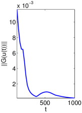
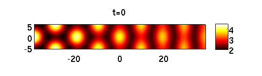
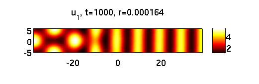
Figure 2: Time integration of (9), $\lambda=2.8,\sigma=0$. (a) time evolution of the residual; (b) initial guess for a front between hexagons and stripes in (9), and the solution at $t=1000$. The latter can be used as starting point for continuation of the stationary problem in, e.g., $\lambda$, which gives a “snaking” branch of stationary fronts. See [11] for further discussion, including the bifurcation of such snaking branches of localized solutions from so–called bean branches. In (b) the horizontal and vertical axes are $x=x_{1}$ and $y=x_{2}$ resp.

Finally, in moviescript.m we give some examples for movie creation. Typically, these require some customized plotsol and plotbra, see mplotsol.m and mplotbra.m, but otherwise explain themselves. See also the end of schnakcmds2.m for time-integration movies.

2.3 Nonlinear boundary conditions (nlbc)

We consider

$$-\Delta u=0\text{ in }\Omega,\quad{\partial}_{n}u+\lambda s(x,y)f(u)=0,$$ (11)

taken from [7], where we choose $s(x,y)=0.5+x+y$, $f(u)=u(1-u)$, and, for diversity, $\Omega=D=\{(x,y)\in{\mathbb{R}}^{2}:\|(x,y)\|_{2}<1\}$. Thus we have the simple linear Laplace equation with nonlinear boundary conditions, where we take $\lambda$ as our bifurcation parameter. Clearly, $u\equiv 0$ and $u\equiv 1$ are two trivial branches, $f(u)>0$ in between, and a crucial feature is that the weight function $s$ changes sign on ${\partial}\Omega$. Moreover, $\left\langle s\right\rangle:=\int_{{\partial}\Omega}sd\Gamma>0$, which corresponds to the case $\left\langle s\right\rangle<0$ in [7]; we chose the different sign to make the connection to the general form (2), ${\bf n}\cdot(c\otimes\nabla u)+qu=g$, of boundary conditions more transparent, i.e., we choose $q=\lambda s(x,y)(1-u)$ and $g=0,c=1$.

As the model is related to gene frequencies, in applications one is mostly interested in solutions $u$ with $0\leq u(x,y)\leq 1$, and in [7] a number of remarkable results are shown, essentially assuming $f$ of the above form and $\left\langle s\right\rangle\neq 0$. In particular, if $\left\langle s\right\rangle>0$ (in our convention), the only nontrivial solutions with $0\leq u(x,y)\leq 1$ in $\Omega$ are on a global branch $u(\cdot;\lambda)$, $\lambda>\lambda_{0}>0$, and these are exponentially stable in the heat equation associated with (11). Additionally, for $0<\lambda\leq\lambda_{0}$, the trivial solution $u\equiv 0$ is stable. We do recover these results numerically, but for completeness we drop the restrictions $\lambda>0$ and $0\leq u(x,y)\leq 1$; note, for instance, that at $\lambda=0$ any constant $u$ is a solution of (11).

The coefficients c=1; a=0; b=0; in fuha.G and in fuha.Gjac are rather obvious, and it remains to encode the boundary conditions in the form (2). The format of the “boundary matrix” bc in the pdetoolbox is rather unhandy, which is why we provide the functions bc=gnbc(neq,varargin) and bc=gnbcs(neq,varargin), see [13, §3.1.4]. Here we need the second version which takes string arguments containing expressions in x,u, and set up fuha.bc as

function bc=nlbc(p,u) % nonlin., x-dep. BC;
lam=u(p.nu+1); enum=max(p.mesh.e(5,:)); % find number of edges
g=mat2str(0);q=[mat2str(lam) ’*(0.5+x+y).*(1-u)’]; bc=gnbcs(p.nc.neq,enum,q,g);

The function fuha.bcjac must provide the coefficients to assemble the $u$ derivatives of the BC. Accordingly,

function bc=nlbcjac(p,u) % generate bc-matrix for derivatives of BC
lam=u(p.nu+1); enum=max(p.mesh.e(5,:));
g=mat2str(0);qj=[mat2str(lam) ’*(0.5+x+y).*(1-2*u)’]; bc=gnbcs(p.nc.neq,enum,qj,g);

With these definitions, (11) can now be run in p2p2 with sw.jac=1 (assembled Jacobians) in a standard way, see nlbccmds.m, and Fig. 3 for some results.

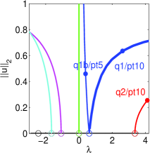
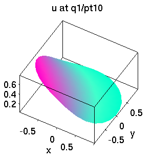
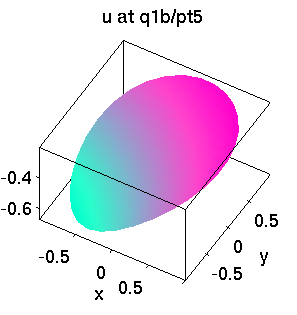
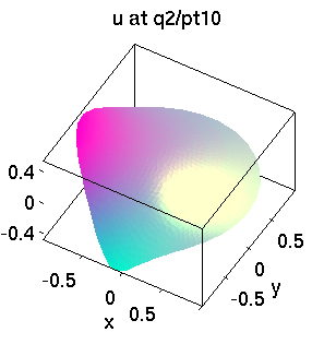
Figure 3: Bifurcation diagram (BD) and example plots for (11). Here at $\lambda_{0}\approx 0.62$ the bifurcation is transcritical, but $0\leq u\leq 1$ holds only on the blue branch to the right of $\lambda_{0}$, i.e. branch q1. $u\equiv 0$ is stable for $0\leq\lambda\leq\lambda_{0}$. At $\lambda=0$ a vertical branch of constant solutions bifurcates, and there are further bifurcation points both for $\lambda<0$ and $\lambda>\lambda_{0}$, but the only non–constant solutions $u$ with $0\leq u\leq 1$ are on q1.

Remark 2.6.

There is less flexibility when using fuha.bcjac for linearizing BC than in using fuha.Gjac for linearizing $G$, as $c$ in (2) is fixed by (1). Thus, essentially bcjac can be used if only $q$ or $g$ in (2) depend on $u$, and in more general cases one has to use sw.jac=0, i.e. numerical differentiation, where fuha.bcjac is not used. On the other hand, in the case of linear homogeneous BC, one has bcjac=bc and hence can set fuha.bcjac=fuha.bc. This is what we do in most examples. $\rfloor$

2.4 Integral constraints: the functionalized Cahn-Hilliard equation (fCH)

As an example of a problem with a constraint we consider the so called functionalized Cahn–Hilliard equation from [2],

$${\partial}_{t}u=-{\cal G}[(\varepsilon^{2}\Delta-W^{\prime\prime}(u)+\varepsilon\eta_{1})(\varepsilon^{2}\Delta u-W^{\prime}(u)+\varepsilon\eta_{d}W^{\prime}(u))],$$ (12)

where $\varepsilon,\eta_{1,2}$ are parameters, $\eta_{d}=\eta_{2}-\eta_{1}$, $W$ is a double–well–potential, typically containing more parameters, with $W^{\prime}(-1)=W^{\prime}(0)=W^{\prime}(u_{+})=0$, for some $u_{+}>0$, and ${\cal G}$ is an operator ensuring mass-conservation, e.g., ${\cal G}f=f-\frac{1}{|\Omega|}\int_{\Omega}f(x)\,{\rm d}x$. In suitable parameter regimes (12) is extremely rich in pattern formation. The basic building blocks are straight (see Fig.4) and curved (see Fig.5 and Fig.6) “channels”, i.e., bilayer interfaces between $u\equiv-1$ and some positive $u$, which show “pearling” and “meander” instabilities, leading to more complex patterns.

Here we explain how to start exploring these with p2p2. Setting $v=\varepsilon^{2}\Delta u-W^{\prime}(u)$, the stationary equation can be written as the two component system

$$-\varepsilon^{2}\Delta u+W^{\prime}(u)+v=0,$$ (13a)

$$-\varepsilon^{2}\Delta v+W^{\prime\prime}(u)v-\varepsilon\eta_{1}v-\varepsilon\eta_{d}W^{\prime}(u)+\varepsilon\gamma=0,$$ (13b)

where $$\gamma \gamma$$ is a Lagrange-multiplier for mass-conservation in (12). We take as an additional unknown, and add the equation

$$q(u):=\int_{\Omega}u\,{\rm d}x-m=0,$$ (13c)

where $m$ is a reference mass, also taken as a parameter. Thus, we now have 4 parameters $(\eta_{1},\eta_{2},\varepsilon,m)$, one additional unknown $\gamma$, and one additional equation $n_{q}=1$. To implement $q$ from (13c), and, strongly recommended, also ${\partial}_{u}q$, we set fuha.qf=@fchqf; fuha.qfder=@fchqjac; and sw.qjac=1. For $W$ we follow [2, §5] and let

$$W(u)=W_{p}(u+1)+20(u-m_{p}+1)^{p+1}H(u-m_{p}+1),\text{ where }W_{p}(u)=\frac{1}{p-2}(pu^{2}-2u^{p})$$

with $m_{p}=(p/2)^{1/(p-2)}$, and $H$ being the Heaviside function. In [2, §5] numerical time integrations are presented with $p=3$, $\varepsilon=0.1$, $\eta_{2}=2$, and $\eta_{1}=1$ (which leads to pearling), resp. $\eta_{1}=2$ (which gives meandering). We aim at similar parameter regimes, but remark that we use somewhat larger $\varepsilon$ to keep numerical costs low in our tutorial setting.

(a) BD	(b)
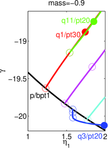
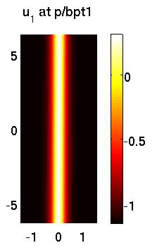
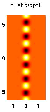
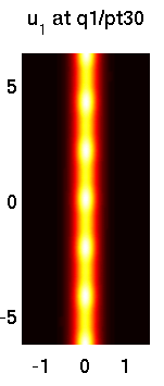
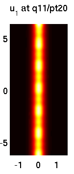
(c)	(d)

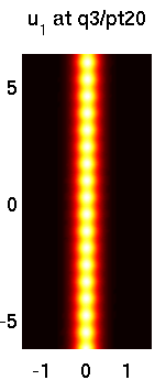
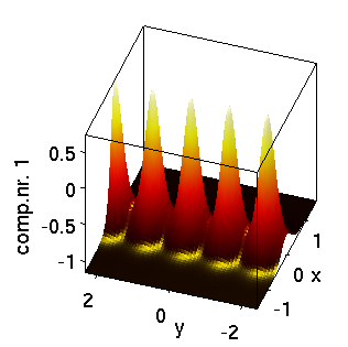
Figure 4: Bifurcations from a straight channel (fchcmds1.m). (a) BD for $\varepsilon=0.35,\eta_{2}=2.5$, $m=-0.9$. (b) $u_{1}$ at 1st BP, tangent direction, pearled branch, and solution on secondary branch. (c) tangent a 3rd BP, and solution on bifurcating branch. Colormap everywhere as in the first plot in (b). In (b) and (c) the horizontal and vertical axes are $x=x_{1}$ and $y=x_{2}$ resp. For (d) see text.

Getting good initial guesses for continuation is a delicate problem for (13). Here we use guesses of the form

$$u_{ig}(x)=-1+(a_{1}+a_{2}\sin(b_{1}y)/\cosh(b_{2}x),\quad v_{ig}=-W^{\prime}(u_{ig})$$ (14)

on rectangular domains $|\Omega|$ with homogeneous Neumann BC for $u$ and $v$, and regular initial meshes of about 8000 points. Moreover, we can either let the software calculate the mass $m=\frac{1}{|\Omega|}\int u(x)\,{\rm d}x$ of the initial guess and use it as the constraint, or give a target $m$ externally.

Figures 4(a)-(c) show some first continuation of and bifurcation from a straight channel, for $\varepsilon=0.35,\eta_{2}=2.5$, fixing $m=-0.9$, primary parameter $\eta_{1}$, and initial guess at $\eta_{1}=1$ of the form (14) with $a_{1}=1.25,a_{2}=0,b_{1}=0,b_{2}=10$. The interfaces between $-1$ and $u_{+}$ and vice versa are rather sharp already for $\varepsilon=0.35$, and only via adaptive mesh–refinement we get a “straight channel” solution from (14), on a grid of about 15.000 triangles. Then increasing $\eta_{1}$ we get a number of “pearling instabilities” and bifurcating pearling branches, which moreover show secondary bifurcations. Interestingly, while the 2nd and 4th primary pearling instabilities have roughly the same wavelengths as the first (see (b)), the 3rd has a much shorter wavelength (see (c)).

As indicated above, slightly changing initial guesses may lead to failure of the initial Newton loop, or to convergence to quite different solutions. As an example we present in Fig. 4(d) the solution for $\varepsilon=0.35,\eta_{1}=1,\eta_{2}=3$ from an initial guess of the form (14) with $a_{1}=1.25,a_{2}=0.25,b_{1}=6,b_{2}=10$, and requiring $m=-0.98$. This directly yields a pearled straight channel.

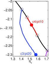
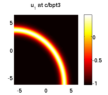
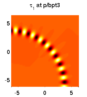
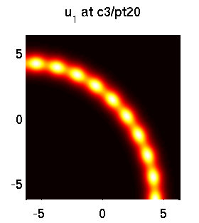
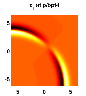
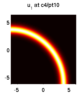
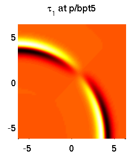
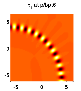
Figure 5: Bifurcation diagram and example directions/solutions for a curved channel. $\varepsilon=0.75,\eta_{2}=2$, and $\eta_{1}=1$ initially, with a quarter-circle channel initial guess with mass $m\approx-0.8675$. On continuation in $\eta_{1}$, the blue branch bifurcates at the 3rd bifurcation point (BP); the first two BPs also yield pearling. The 4th and 5th BPs are connected by a “meandering” branch, and the 6th BP yields pearling again. The horizontal and vertical axes in the solution plots are $x=x_{1}$ and $y=x_{2}$ resp. See fchcmds2.m.

Getting a curved channel from (a curved version of) an initial guess like (14) turns out to be difficult for small $\varepsilon$. Figure 5 shows an example obtained after some trial and error (where the Newton loop often gets stuck at residuals of about $10^{-4}$ or $10^{-5}$), after mesh–refinement to about 25.000 triangles, but with still rather large $\varepsilon=0.75$. After having found some curved solution (on the black branch), we can continue it to smaller $\varepsilon$, which, however, needs more mesh refimement, and the bifurcation scenario does not change much compared to the case $\varepsilon=0.75$ in Fig. 5.

Finally, in fchcmds3.m we give firstly a curved channel obtained by first using Matlab’s fsolve on an initial guess, see Fig. 6 (a), and secondly a channel with a sharp bend as an initial guess that leads to spots, Fig. 6 (b).

Remark 2.7.

As the fCH examples are rather slow, in the cmds files we often set p.nc.ntot to a rather small number, e.g., p.nc.ntot=20, and we often switch off bifurcation detection and localization on bifurcating branches. When using these files as templates, this very likely needs to be reset. $\rfloor$

(a)	(b)

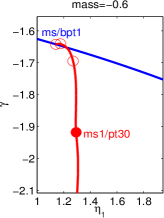
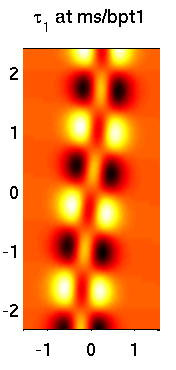
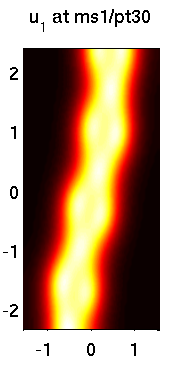
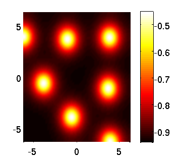
Figure 6: (a) Bifurcation from a “thick” meandering branch. $(\varepsilon,\eta_{3},m)=(0.35,3,-0.6)$, initially $\eta_{1}=1$ and initial guess of type (14) with $a=1.25,a_{2}=0.3,b_{1}=0.5,b_{2}=10$. Note that the tangent at bifurcation is different from the previous pearling in the sense that it also has a transversal periodic structure. (b) $u$ for spots obtained from a “sharp bend” initial guess, $(\eta_{1},\eta_{2},\varepsilon)=(1,2,0.8)$, $m\approx-0.85$. See fchcmds3.m for details. The horizontal and vertical axes in the solution plots are $x=x_{1}$ and $y=x_{2}$ resp.

2.5 Phase equation for traveling waves

Systems (1) with continuous symmetries require the selection of a particular group element in order to allow for a continuation approach since otherwise the linearization $\partial_{u}G$ has a kernel. This can often conveniently be done by adding a suitable constraint, such as the norm constraint in (7) for the scaling symmetry in the eigenvalue problem. Note that although the discretization error may eliminate the kernel, such that the continuation works, it is essentially uncontrolled and correct resolution of parameter dependencies requires a modification.

A traveling wave $u$ on an infinite strip $\Omega={\mathbb{R}}\times(-L,L)$ possesses a translation symmetry in $x$-direction with kernel of $\partial_{u}G(u)$ generated by the spatial derivative $\partial_{x}u$. The selection of a fixed translate is naturally done by (i) adding a comoving frame term $s\partial_{x}u$ to (1), that is, by modifying the tensor $b$ with an additional parameter $s$, and (ii) adding an auxiliary equation that constrains the continuation path to be orthogonal to the group orbit: $\langle\partial_{\lambda}u,\partial_{x}u\rangle_{2}=0$. Numerically, we discretize the derivative in the continuation direction $\partial_{\lambda}u\approx(u_{\rm old}-u)/(\lambda_{\rm old}-\lambda)$, where the subscript ‘old’ refers to the previous continuation step (saved in p.u in p2p2). Since the division by $\lambda_{\rm old}-\lambda$ is redundant, we obtain the auxiliary equation

$$\langle\partial_{x}u,u_{\rm old}-u\rangle_{2}=0.$$

For the benefit of a simpler derivative of the resulting $G$ with respect to $u$ one may also use $\langle\partial_{x}u_{\rm old},u_{\rm old}-u\rangle_{2}=0$ since these are equivalent in the continuum limit. In the case of periodic boundary conditions in the $x$-direction we have $\langle\partial_{x}u,u\rangle=0$ such that the conditions simplify to

$$\langle\partial_{x}u,u_{\rm old}\rangle=0 \langle\partial_{x}u_{\rm old},u\rangle=0$$ or ,

respectively. See, e.g., demo schnaktravel for an implementation in p2p2.

On the other hand, with the separated boundary conditions in Matlab’s pdetoolbox the translation symmetry never appears, but the constraining procedure still allows to model the real line. For illustration, consider fronts, which are spatially heteroclinic connections to homogeneous steady states. In this case a sufficiently long $\Omega$ in the $x$-direction and homogeneous Neumann BC at the end sides is (generically) a small perturbation to the front profile, also for a traveling front with $s$ chosen as the wave speed. Continuation in a parameter $\lambda$ of $G$ is now typically possible, which means fixed speed $s$. But on the infinite strip the speed $s$ will typically depend on $\lambda$. This is resolved by a constraint as described above, which (implicitly) couples $s$ and $\lambda$, so that continuation of the extended system in $\lambda$ with additional unknown $s$ calculates their interdependence. In §2.6 we show how periodic domains can be implemented in p2p2 such that translation symmetry can be realized (e.g. for periodic or localized traveling waves) and a priori requires the constraint.

Example: Traveling fronts in an Allen-Cahn model (acfront).

For illustration of the simplest setting, consider the Allen-Cahn equation $\partial_{t}u=\Delta u+\lambda u(1-u)(\mu+u)$, whose traveling waves with speed $s$ in $x$-direction solve the elliptic equation

$$-\Delta u-\lambda u(1-u)(\mu+u)-s\partial_{x}u=0.$$

The (explicitly known) quasi 1D traveling front solutions are near a $y$-independent heteroclinic connection from $-\mu$ to $1$. With domain $\Omega$ set to a finite rectangle with homogeneous Neumann BC  we detect near-front solutions as follows. For $\mu=1$ the nonlinearity is symmetric and waves stationary. Increasing $\lambda$ from $1$ yields a pitchfork bifurcation to half cosine-modes that approach a heteroclinic connection between $\pm 1$ as $\lambda$ increases further. Next we add the constraint and the parameter $s$ and perform a continuation in the symmetry breaking parameter $\mu$. The bifurcation diagrams (see acfront_cmds) match the explicitly known dependence of $s$ on $\mu$, e.g. [6].

2.6 Periodic boundary conditions for rectangular domains

For axis-aligned rectangular domains p2p2  can identify opposite sides with equal grid arrangements in order to generate cylindrical or toroidal geometry. The initial setup requires homogeneous Neumann boundary conditions on the sides that are to be identified, and the grid requirement is most easily realized with a mesh from poimesh. The boundary conditions on the remaining boundary can be arbitrary. For all calculations the effective mesh is reduced by removing the points from one of the identified sides of the rectangle such that the solution vector p.u is smaller than on the initial mesh. However, the full mesh and the Neumann BC are used for assembling the FEM discretized PDE and for plotting purposes.

The transformation of a vector from the reduced to the full mesh goes by the matrix p.mat.fill, which simply extends a vector by generating copies of entries on the periodic boundary. For instance, p.mat.fill*p.u(1:p.nu) gives the extended solution vector.

The switch to periodic domains in p2p2 can be conveniently done by calling the routine rec2per with additional argument to determine the type of periodic domain:

1: top=bottom side, 2: left=right side, 3: torus (this setting is stored in p.sw.bcper).

The convenience function rec2perf in addition loads a point from a Neumann BC  solution from a file for the purpose of continuing from this solution with periodic BC.

These routines essentially generate the matrix p.mat.fill, which is set to $1$ in the standard (non-periodic) setting. In addition these routines modify a given solution from the Neumann domain to the periodic domain by removing the redundant entries from p.u with the matrix p.mat.drop via p.mat.drop*p.u(1:p.nu); also the degree of freedom parameter p.nu is set to the corresponding (smaller) value.

Next, we explain the details of the transformation of the system matrices from Neumann to periodic BC and provide an example in §2.6.2.

Remark 2.8.

Remark 2.3 also applies to these matrices p.mat.XX so that they are not saved to disk. In order to avoid miscalculations upon reloading, for periodic geometries p.mat.fill and p.mat.drop are saved as empty arrays [] (for non-periodic domains these are saved as $1$); an attempt to run a problem from a periodic domain without resetting the matrices will then produce an error message. The matrices are automatically regenerated when loading a point with loadp, which uses the geometry type stored in p.sw.bcper. $\rfloor$

Remark 2.9.

Grid adaption for periodic domains is so far implemented only in a simple ad hoc way: to ensure that identified boundaries match after grid adaption, we remove triangles from a refinement–list generated by pdeadworst. This is controlled by p.nc.bddistx, p.nc.bddisty, see rmbdtri.m for details. Thus, for periodic domains, mesh adaption is useful only as long as there are no large gradients near the identified domain boundaries. $\rfloor$

2.6.1 Transforming the FEM problem from Neumann to periodic BC.

For illustration, consider the simple situation of a one-dimensional chain with 4 elements. In that case node 1 and 4 are identified to generate a ring and we have

$$\texttt{p.mat.fill}=\begin{pmatrix}1&0&0\\ 0&1&0\\ 0&0&1\\ 1&0&0\end{pmatrix},\quad\texttt{p.mat.fill'}=\begin{pmatrix}1&0&0&1\\ 0&1&0&0\\ 0&0&1&0\end{pmatrix},\quad\texttt{p.mat.drop}=\begin{pmatrix}1&0&0&0\\ 0&1&0&0\\ 0&0&1&0\end{pmatrix}.$$

Hence, p.mat.fill writes a copy of entry 1 into slot 4 while p.mat.fill’ adds entries 1 and 4 into slot 1, and p.mat.drop simply removes the last entry. Note that in the actual matrix construction it is not assumed that the points that are to be identified appear within p.u in any specific ordering.

Next, observe that the piecewise linear ‘hat’ basis function at a node is the sum of its triangular parts over the neighboring triangles. At a boundary node the basis function for homogeneous Neumann conditions simply does not have an additive contribution from outside the grid. Therefore, it can be extended to a full basis function of an interior node in the periodic domain by adding the corresponding contributions from periodically identified nodes. Denote the basis functions for the Neumann problem by $(\phi_{j})_{j=1}^{n_{p}}$ and those for the periodic problem by $(\psi_{j})_{j=1}^{n_{p}^{\text{per}}}$ with $n_{p}^{\text{per}}<n_{p}$. For the above 1D example $n_{p}=4,n^{\text{per}}_{p}=3,\psi_{1}=\phi_{1}+\phi_{4},\psi_{2}=\phi_{2}$, and $\psi_{3}=\phi_{3}$. Considering for simplicity the mass matrix (denoted by $M$in the Neumann case and $M^{\text{per}}$ in the periodic case), we have $M_{ij}=\langle\phi_{i},\phi_{j}\rangle_{2}$ and $M^{\text{per}}_{ij}=\langle\psi_{i},\psi_{j}\rangle_{2}$ such that

$$M^{\text{per}}_{ij}=M_{ij}\quad\text{for}\ 2\leq i,j\leq 3$$

$$M^{\text{per}}_{1j}=M_{1j}+M_{4j},\ M^{\text{per}}_{j1}=M_{j1}+M_{j4},\quad\text{for}\ 2\leq j\leq 3$$

$$M^{\text{per}}_{11}=M_{11}+M_{14}+M_{41}+M_{44}.$$

The modification of the Neumann stiffness matrix $K$ to the periodic stiffness matrix $K^{\text{per}}$ is completely analogous. The right hand side $F$ satisfies

$$F^{\text{per}}_{j}=F_{j}\quad\text{for}\ 2\leq j\leq 3,\ F^{\text{per}}_{1}=F_{1}+F_{4}.$$

These transformations are efficiently performed via

Kper	= p.mat.fill’ * K * p.mat.fill
Mper	= p.mat.fill’ * M * p.mat.fill
Fper	= p.mat.fill’ * F.

In practice we assemble $K,M$ and $F$ via the Matlab pdetoolbox and apply the above transformation.

In order to account for the dependence of $c,b,a,f$ in (1) on p.u, the vector p.mat.fill*p.u is fed into the Neumann BC assembling routines. Recall that the matrices p.mat.fill and p.mat.drop are generated automatically by the routine rec2per according to the value of p.sw.bcper.

2.6.2 Cylinder geometry: Quasi-1D traveling waves (schnacktravel)

For the simplest illustration of cylinder geometries we consider a quasi 1D setting in the Schnakenberg model (9) with $\sigma=0$, $\Omega=(-0.1,0.1)\times(-L,L)$ and full Neumann boundary conditions at first. Based on expectations of the general structure of the existence region for wavetrains in such systems [9, 3], we follow a certain continuation path in $(\lambda,L)$ that leads to a travelling wave bifurcation. First we choose the domain length $L=L_{c}$ compatible with the Turing instability mentioned in §2.2: this occurs at $\lambda_{c}=\sqrt{d}\sqrt{3-2\sqrt{2}}\approx 3.2085$ with spatial period $L_{c}=2\pi/k_{c}$, $k_{c}=\sqrt{\sqrt{2}-1}$.

For decreasing $\lambda$ from, say $\lambda=3.5$, the instability appears as a pitchfork bifurcation under Neumann BC and we continue the resulting branch until $\lambda=1.3$. See Figure 7(a). This value is somewhat arbitrarily chosen from the expectation that for sufficiently small $\lambda$, increasing the domain length yields a fold and traveling wave bifurcation for the associated wavetrains. To change the domain length, we multiply both diffusion constants by a factor $\rho$, i.e. $L=\pi/(\sqrt{\rho}k_{c})$. Now we switch the continuation parameter to $\rho$ and continuation starting from the endpoint of the previous continuation indeed leads to a fold. See Figure 7(b). Note that the bifurcation point marked with a circle does not give traveling waves on ${\mathbb{R}}$ as it stems from Neumann BC. This is because there is no extension of the Neumann solution from the bounded domain onto ${\mathbb{R}}$.

(a)	(b)	(c)	(d)

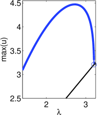
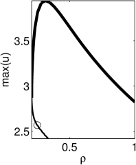
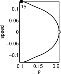
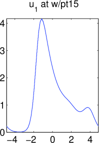
Figure 7: (a) Bifurcation of stripes under Neumann BC  through a Turing instability. (b) Continuation from endpoint of (a) in the domain length parameter $\rho=(L_{c}/L)^{2}$. Here the circle marks a bifurcation under Neumann BC. The traveling wave bifurcation under periodic BC  is closer to the fold point. (c) Bifurcation diagram in cylindrical geometry with parameters $\rho$ and speed $s$. (d) profile for the solution at point 15 marked in (c).

After these preparatory steps we change the geometry to a cylinder such that the boundaries at $-L$ and $L$ are identified. As described in §2.5, we add a phase equation to eliminate the zero eigenvalue from translation symmetry and add the traveling wave speed as a second parameter to the active continuation parameters. Finally, we load the endpoint from the previous calculation. These steps are conveniently done in the schnaktravel demo by the following commands:

r=rec2perf(’q2’,’pt25’,’r’,1);  % load ’q2/pt25’, set directory name ’r’, geometry type 1
r.nc.ilam=[3;2];                % set parameters with indices 3 and 2 as active
r.nc.nq=1; r.fuha.qf=@schnakqf; % set number auf aux. eqn. and function handle
p.sw.qjac=1; p.fuha.qfder=@schnak_qfder;         % analytical jac for aux. eqn.

Here the new primary parameter has index 3, which corresponds to the traveling wave speed $s$ in the comoving frame term $s\partial_{y}(u,v)^{T}$ added to (1); see §2.5. Now we perform a continuation from the endpoint of the Neumann BC computations back for decreasing $\rho$. The stationary solution branch is the same, but the location of the bifurcation point changed to a value much closer to the fold point. Branch switching in both directions and continuation yields the branches and profile plotted in Figure 7(c),(d).

2.6.3 2D traveling waves in a cylinder (twofluid)

A traveling wave problem that cannot be reduced to a one dimensional problem occurs in the ‘two-fluid’ tokamak plasma model from [14]. The profile satisfies the elliptic problem

$$0 =-\nu\Delta u_{1}-(\nabla V)^{\perp}\cdot\nabla u_{1}-(\delta+s)\partial_{x_{2}}u_{1}+\partial_{x_{2}}V/L_{1},$$ (15)

$$0 =-\nu\Delta u_{2}-(\nabla V)^{\perp}\cdot\nabla u_{2}-s\partial_{x_{2}}u_{2}-\partial_{x_{2}}V/L_{1},$$

$$0 =-\Delta V-u_{1}-u_{2}$$

posed on $\Omega=(-1,1)^{2}$ subject to periodic BC  in the second variable $x_{2}$ and homogeneous Dirichlet BC in $x_{1}$, with parameters $\nu,\delta,L_{1}>0$. For definiteness we fix $L_{1}=2$ and $\nu=9\cdot 10^{-4}$, and take $\delta$ as primary parameter.

As proven in [14], in the parabolic problem the trivial state $u_{1}=u_{2}=V=0$ for $s=0$ undergoes a generic supercritical Hopf bifurcation for decreasing $\delta$ at $\delta=\delta_{2}\approx 0.16$ and this generates periodic traveling waves. However, using the knowledge of $s$ at onset, the bifurcation has a double zero eigenvalue and hence cannot be detected by the standard bifdetec. Instead, we set $s$ at the onset speed and $\delta$ just below the bifurcation value, and perturb the trivial solution by a rough eigenfunction. Using time evolution with tint, the trajectory indeed approaches the stable traveling wave solution. A Newton-loop for the system augmented by the phase equation from §2.5 then yields an initial solution to (15). In Figure 8 we plot some resulting branches and solutions.

Remarkably, we find solutions on the blue branch for values of $\delta$ larger than the bifurcation point. It thus coexists with the locally stable trivial state, which is proven to be globally stable for $\delta>5\delta_{2}$ in [14]. This numerical result thus shows that failure to prove global stability of the trivial state for $\delta\in(\delta_{2},5\delta]$ is not a technicality: there is a branch of nontrivial solutions preventing global stability for some range above $\delta_{2}$.

(a)	(b)	(c)	(d)

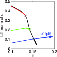
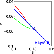
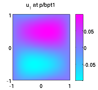
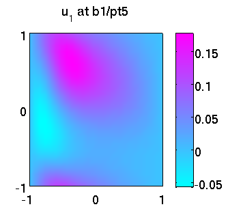
Figure 8: (a),(b) Bifurcation diagrams. (c),(d) Contour plots of $u_{1}$-component for solutions.

2.6.4 Torus geometry: nonlinear Bloch waves (nlb)

As a second example for periodic boundary conditions we consider the time harmonic Gross-Pitaevskii equation

$$-\Delta\phi-\omega\phi+V(x)\phi+\sigma|\phi|^{2}\phi=0,\quad x\in{\mathbb{R}}^{2}$$ (16)

with the periodic potential $V(x+2\pi e_{m})=V(x)$ for all $x\in{\mathbb{R}}^{2}$ and $m=1,2$, where $e_{m}$ is the $m$-th Euclidean unit vector in ${\mathbb{R}}^{2}$, and $\sigma=\pm 1$. Equation (16) describes, e.g., time harmonic electromagnetic fields in nonlinear photonic crystals or Bose-Einstein condensates loaded on optical lattices. It has quasi–periodic solutions bifurcating from the trivial solution at spectral points $\omega_{*}\in\text{spec}(-\Delta+V)$, see [4, 5]. Here we consider the particular case where $\omega_{*}=\omega_{n_{*}}(k_{*})$ for some fixed $k_{*}\in(-1/2,1/2]^{2}$, with $\omega_{n_{*}}$ the $n_{*}$-th band function in the band structure $(\omega_{n}(k))_{n\in{\mathbb{N}}}$, $k\in(-1/2,1/2]^{2}$. Thus we seek a quasi-periodic nonlinear Bloch-wave $\phi$ of (16) with the quasi-periodicity vector $k_{*}$, i.e., $\phi(x)=e^{{\rm i}k_{*}\cdot x}\eta(x),\eta(x{+}2\pi e_{m})=\eta(x)\text{ for all }x{\in}{\mathbb{R}}^{2},m=1,2.$ As shown in [5], for $\omega=\omega_{*}+\text{sign}(\sigma)\varepsilon^{2}$ with $\varepsilon>0$ small enough such nonlinear Bloch waves exist and have the asymptotics

$$\phi(x)\sim\varepsilon\left(|\sigma|\|p_{n_{*}}(\cdot,k_{*})\|_{L^{4}((-\pi,\pi)^{2})}^{4}\right)^{-1/2}p_{n_{*}}(x,k_{*})e^{{\rm i}k_{*}\cdot x} \varepsilon\to 0.$$ for (17)

Inserting $\phi(x)=e^{{\rm i}k_{*}\cdot x}\eta(x)$ in (16) and using real variables $u_{1},u_{2}$, i.e., $\eta=u_{1}+{\rm i}u_{2}$, we get

$$0=G(u_{1},u_{2}):=-\begin{pmatrix}\Delta u_{1}\\ \Delta u_{2}\end{pmatrix}+2\begin{pmatrix}k_{*}\cdot\nabla u_{2}\\ -k_{*}\cdot\nabla u_{1}\end{pmatrix}+(|k_{*}|^{2}-\omega+V(x))\begin{pmatrix}u_{1}\\ u_{2}\end{pmatrix}+\sigma(u_{1}^{2}+u_{2}^{2})\begin{pmatrix}u_{1}\\ u_{2}\end{pmatrix},$$ (18)

on the torus $\mathbb{T}^{2}={\mathbb{R}}^{2}/(2\pi{\mathbb{Z}}^{2})$, with linerization

$$Lu=-\begin{pmatrix}\Delta u_{1}\\ \Delta u_{2}\end{pmatrix}+2\begin{pmatrix}k_{*}\cdot\nabla u_{2}\\ -k_{*}\cdot\nabla u_{1}\end{pmatrix}+(|k_{*}|^{2}-\omega+V(x))\begin{pmatrix}u_{1}\\ u_{2}\end{pmatrix}$$

around $0$. We aim to find bifurcations from the branch $u{=}0$, with primary parameter $\omega$.

(18) has the continuous symmetry $u\mapsto\bigl{(}\begin{smallmatrix}\cos\alpha&-\sin\alpha\\ \sin\alpha&\cos\alpha\end{smallmatrix}\bigr{)}u$ from the phase invariance $\phi\mapsto{\rm e}^{{\rm i}\alpha}\phi$ of (16). In particular, each eigenvalue $\mu$ of $L$ is double: if $Lu=\mu u$, then also, e.g., $Lv=\mu v$ with $v=(-u_{1},u_{2})$ which is linearly independent of $u$. To deal with this phase invariance we proceed as follows. First we modify findbif.m to search for $\omega$ values where two eigenvalues go through zero; see findbifm.m, which can easily be generalized to $m$ eigenvalues going through zero. Next we modify swibra.m to a version swibram.m. Here, the user first has to choose which of the two zero eigenvalues to use for bifurcation, and second, has to set a “phase-fix-factor” ${\tt pffac}=\gamma\neq 0$.

For $\gamma=0$, branch–switching proceeds as usual: swibram produces a new tangent $\tau$, from which we may continue a bifurcating branch using cont, with one caveat. During continuation, the phase $\alpha$ of the solution, for instance defined as $\alpha=\arctan\frac{u_{2}(x_{*})}{u_{1}(x_{*})}$ at one point $x_{*}$ in the domain, may change in an uncontrolled way, strongly dependent, for instance, on the step–length.

For $\gamma\neq 0$, the software removes this undesired phase–wandering by fixing $u_{2}(x_{*})=0$ at a point $x_{*}$ where $|u_{1}(x_{*})|$ (i.e., the absolute value of the real part) is maximal. If $\gamma<0$, this is achieved by the method (a), where $u_{2}(x_{*})$ is set to $0$ and $u_{2}(x_{*})$ as well as the equation for $u_{2}(x_{*})$ are dropped from the discretized system. For this we use modifications of p.mat.drop and p.mat.fill, see dropp.m.

If $\gamma>0$ is chosen, the following method (b) is used. Assume that $x_{*}$ is point ${\tt p.pfn}=n_{*}$ in the discretization. We then overload pderesi.m locally to replace the $n_{u}/2+n_{*}$ entry r(p.nu/2+p.pfn) in $G(u)$ by $\gamma u(n_{u}/2+n_{*})$, i.e., r(p.nu/2+p.pfn)=p.pffac*u(p.nu/2+p.pfn); where p.pffac=$\gamma$. Accordingly we also overload getGupde.m locally and add:
Gu(p.nu/2+p.pfn,:)=zeros(1,p.nu); Gu(p.nu/2+p.pfn,p.nu/2+p.pfn)=p.pffac;

In swibram.m we thus use method (a) if ${\tt p.pffac}<0$ (with the precise value irrelevant) and method (b) if ${\tt p.pffac}>0$ (with for instance $\gamma=10^{3}$). Both methods yield indistinguishable results for all our tests.

For a numerical example we choose $\sigma=-1$, the potential $V(x)=e^{-x_{1}^{2}}\cos(x_{2}),\ x\in(-\pi,\pi]^{2}$ and $k_{*}=(1/2,1/2)$. Figure 9 shows the first three bifurcating branches, and real parts of selected profiles. For all three branches we obtain excellent agreement with the asymptotics (17). The mesh was generated by poimesh. Though time is not crucial here, for illustration we precompute ${\tt pot}:=V$ resp. its interpolation poti to the triangle centers (needed in mesh-refinement) and put these fields into p.mat. As p.mat is not saved to disk, we then also need to overload loadp.m locally, and also recompute p.mat.pot and p.mat.poti after mesh–refinement, see nlbpmm.m. See also the end of cmds.m for an example of mesh-refinement following Remark 2.8.

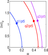
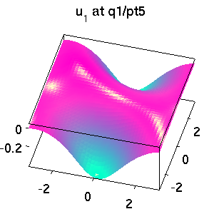
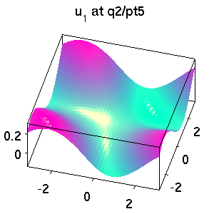
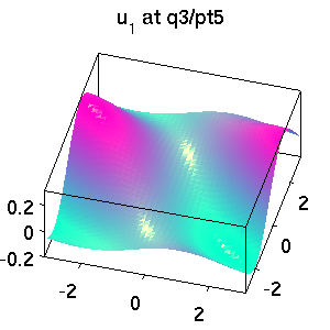
Figure 9: Nonlinear Bloch wave example for $V(x)=e^{-x_{1}^{2}}\cos(x_{2})$ and $k_{*}=(1/2,1/2)$.

2.7 Other examples from [13]

The root demo directory p2p2/demos also contains transfers of the examples from [13] to the new setup, e.g:

• acgc: the (cubi–quintic) Allen–Cahn with Dirichlet BC and a global coupling, i.e.,

  $$-0.1\Delta u-u-u^{3}+u^{5}-\lambda\left\langle u\right\rangle=0,$$

  where $\left\langle u\right\rangle=\int_{\Omega}u\,{\rm d}x$. This uses some modifications of the linear system solvers.

• bratu: a scalar elliptic equation on the unit square with zero flux BC

  $$-\Delta u-f(u,\lambda)=0,\quad f(u,\lambda)=-10(u-\lambda{\rm e}^{u}),$$

  for which a number of results can be obtained analytically. The updated demo contains a branch point continuation, see §2.1.4.

• chemtax: a quasi–linear non–diagonal reaction–diffusion system from chemotaxis in the form

  $$G(u,\lambda):=-\begin{pmatrix}D\Delta u_{1}-\lambda\nabla\cdot(u_{1}\nabla u_{2})\\ \Delta u_{2}\end{pmatrix}-\begin{pmatrix}ru_{1}(1-u_{1})\\ \frac{u_{1}}{1+u_{1}}-u_{2}\end{pmatrix}=0.$$ (19)

• rbconv: Rayleigh-Bénard convection in the Boussinesq approximation streamfunction form

  $$-\Delta\psi+\omega =0,$$

  $$-\sigma\Delta\omega-\sigma R\partial_{x}\theta+\partial_{x}\psi\partial_{z}\omega-\partial_{z}\psi\partial_{x}\omega =0,$$ (20)

  $$-\Delta\theta-\partial_{x}\psi+\partial_{x}\psi\partial_{z}\theta-\partial_{z}\psi\partial_{x}\theta =0,$$

  and with various boundary conditions. (The implementation given here detects both branches of the stress-free BC by continuation – in [13] we used tint to detect the second branch.)

• gpsol: time–harmonic Gross–Pitaevskii equations in a rotating frame, leading to real systems of the form

  $$-\Delta u+(r^{2}-\mu)u-|U|^{2}u-\omega(x{\partial}_{y}v-y{\partial}_{x}v)=0,$$ (21a)

  $$-\Delta v+(r^{2}-\mu)v-|U|^{2}v-\omega(y{\partial}_{x}u-x{\partial}_{y}u)=0,$$ (21b)

  where $|U|^{2}=u^{2}+v^{2}$, and generalizations to more components. This is similar to (18), but here we use potentials $V(x,y)=x^{2}+y^{2}$, and search for and continue soliton solutions.

• vkplate: the Von Kármán equations for the buckling of elastic plates

  $$\begin{split}-\Delta^{2}v-\lambda{\partial}_{x}^{2}v+[v,w]&=0,\quad-\Delta^{2}w-\frac{1}{2}[v,v]=0,\end{split}$$ (22)

  where $[v,w]:=v_{xx}w_{yy}-2v_{xy}w_{xy}+v_{yy}w_{xx}$, with various boundary conditions. After some transformations this yields a 10-equations-system of the form (1).

In general, the transfer is rather straightforward, and here we only give some details on the new implementation of vkplate which is our most complicated example with respect to coding. Mainly we want to illustrate how to gain additional flexibility in the sfem=1 setup by modifying setfemops.m. This is needed if a parameter genuinely enters, for instance, the stiffness matrix $K$, as does $\lambda$ in vkplate. Similar ideas are also used in, e.g., gpsol and rbconv. See also Remark 2.2.

2.7.1 Semilinear setting for Von Kármán equations (vkplate)

In [13] we rewrite (22) as a system of 10 equations, where the (bifurcation) parameter $\lambda$ enters the stiffness matrix. In order to treat this in the sfem=1 setting, we essentially put the tensors a and c into p.eqn.a, p.eqn.c, with one little trick: the $\lambda$ dependent part is not put into p.eqn.c, but (with $\lambda=1$) into an extra field p.eqn.c2. We then locally modify setfemops.m to also assemble the associated stiffness matrix p.mat.K2, and set up vksG as, essentially,
r=(p.mat.K+lam*p.mat.K2)*u(1:p.nu)-p.mat.M*f; The encoding of ${\partial}_{u}G(u)$ then also requires a little care, see the listing below.

function p=setfemops(p) % modified for vkplate: generate additional K2 which
% will be multiplied by lam in vksG and vksGjac
upde=p.mat.fill*p.u(1:p.nu); neq=p.nc.neq; bc=p.fuha.bc(p,p.u); m=p.mesh;
[~,p.mat.M,~,~,p.mat.bcG,~,~]=assempde(bc,m.p,m.e,m.t,0,1,zeros(neq,1),upde);
[p.mat.K,~]=assempde(bc,m.p,m.e,m.t,p.eqn.c,p.eqn.a, zeros(neq,1),upde);
[p.mat.K2,~]=assema(m.p,m.t,p.eqn.c2,0,zeros(neq,1));
end

function Gu=vksGjac(p,u)  % sfem=1 jacobian for von karman-plate
lam=u(p.nu+1); n=p.np; u5=u(4*n+1:5*n); u6=u(5*n+1:6*n);
u7=u(6*n+1:7*n); u8=u(7*n+1:8*n); u9=u(8*n+1:9*n); u10=u(9*n+1:10*n);
f2u5=spdiags(-u9,0,n,n); f2u6=spdiags(-u8,0,n,n); f2u7=spdiags(2*u10,0,n,n);
f2u8=spdiags(-u6,0,n,n); f2u9=spdiags(-u5,0,n,n); f2u10=spdiags(2*u7,0,n,n);
f4u5=spdiags(u6,0,n,n); f4u6=spdiags(u5,0,n,n); f4u7=spdiags(-2*u7,0,n,n);
zd=spdiags(zeros(n,1),0,n,n); % 0-diag for easy sorting of non-zeros into Fu
Fu=[sparse([],[],[],n,10*n,0);
    [zd zd zd zd f2u5 f2u6 f2u7  f2u8  f2u9 f2u10];
    sparse([],[],[],n,10*n,0);
    [zd zd zd zd f4u5 f4u6 f4u7   zd    zd   zd];
    sparse([],[],[],6*n,10*n,0)];  % set remainder of Fu to 0
Gu=p.mat.K+lam*p.mat.K2-p.mat.M*Fu;
end

3 Discussion and outlook

Compared to the version of pde2path documented in [13], p2p2 brings a number of

1. extensions, e.g.: fold–and branchpoint continuation, general auxiliary equations, periodic boundary conditions, interface to fsolve,

2. optimizations, e.g.: faster FEM in the sfem=1 setting,

3. cleanups, reorganizations, improved user–friendliness, e.g.: substructures of p, no single explicit parameter $\lambda$ anymore, but easy switching between different parameters, improved plotting,

and some bug-fixes (not documented in detail here). Moreover, besides the tutorial examples given here and in [13], pde2path and p2p2 have been applied to a number of genuine research problems, e.g., [5, 11, 12, 14], and a number of further projects are in progress. Often, new projects require extensions of the software, and while (i) clears point 2 from the To-Do-List in [13, §6], the list as such has rather become longer. Currently, we are working on or planning the following extensions:

1. Implement some more general (stationary) bifurcation handling, including branch–switching at multiple bifurcations; for the case of double eigenvalues due to phase–invariance this has been done in an ad–hoc way in §2.6.4. Also, Hopf bifurcations will be tackled. These points still roughly correspond to [13, Point 1. in §6].

2. Invariant subspace continuation, e.g., [1]; the goal is to track the small eigenvalues in an efficient way, and to check the performance of other test functions as an alternative to the determinant of the (extended) Jacobian or the number of eigenvalues with negative real–parts used so far (see [13, §2.1,§3.1.6]).

3. There are function handles p.fuha.lss and p.fuha.blss for solving the linear systems and the extended linear systems that occur in Newton loops and, e.g., for calculating new tangent predictors. However, except for some Sherman–Morrison formulas for the case of an Allen–Cahn equation with global coupling [13, §3.5], we always use the standard solvers lss.m and blss.m, which simply call Matlab’s $\backslash$ operator. So far, this turned out superior to iterative solvers, but this seems to change for very large systems, in particular in 3D, see 5 below, and in summary some iterative solvers and customized solvers for bordered systems will be fitted into p2p2 as well.

4. A Matlab environment online help for p2p2 should be coming soon.

5. The basic functionality of p2p2 has already been ported to 3D, based on the free Matlab FEM package OOPDE, [8]. In particular, this gives identical user interfaces in 2D and 3D. In the long term, the 2D, 3D (and also 1D) versions shall merge to a single package. This is partly similar to the philosophy of COCO [10].

As pde2path is and will remain an “open project”, comments and help on any of the above points will be very welcome. Please send questions, remarks or requests to pde2path@uni-oldenburg.de or to any of the authors.

Appendix A Tables of p2p2 functions, controls, switches and fields

In this appendix, intended as a reference card, we give overviews of the main p2p2 functions (see the files in p2plib for more comments), and of the basic p2p2 structure p and the contents of its fields.

Table 2: Main fields in the structure p describing a p2p2 proplem; see stanparam.m in p2plib for detailed information on the contents of these fields and the standard settings. The destinction between nc and sw is somewhat fuzzy, as both contain variables to control the behaviour of the numerics: the rule is that nc contains numerical constants, real or integer, while the switches in sw only take a finite number of values like 0,1,2,3. Finally, u,np,nu,tau and branch are not grouped into a substructure as, in our experience, these are the variables most often accessed directly by the user.

field	purpose
fuha	struct of function handles; in particular the function handles p.fuha.G, p.fuha.Gjac, p.fuha.bc, p.fuha.bcjac defining (1) and Jacobians, and others such as p.fuha.outfu, p.fuha.savefu, …
nc, sw	numerical controls such as p.nc.tol, p.nc.nq, …, and switches such as p.sw.bifcheck,…
u,np,nu	the solution u (including all parameters/auxiliary variables in u(p.nu+1:end)), the number of nodes p.np in the mesh, and the number of nodal values p.nu of PDE–variables
tau,branch	tangent tau(1:p.nu+p.nc.nq+1), and the branch, filled via bradat.m and p.fuha.outfu.
sol	other values/fields calculated at runtime, e.g.: ds (stepsize), res (residual), …
usrlam	vector of user set target values for the primary parameter, default usrlam=[];
eqn,mesh	the tensors $c,a,b$ for the semilinear FEM setup, and the geometry data and mesh.
plot, file	switches (and, e.g., figure numbers and directory name) for plotting and file output
time, pm	timing information, and pmcont switches
fsol	switches for the interface to fsolve, see Remark 2.
mat	problem matrices, e.g., mass/stiffness matrices $M$, $K$ for the the semilinear FEM setting, and drop and fill for periodic BC; by default, mat is not saved to disk, see also Remark 4.

Table 3: Main p2p2 functions for user calls; some of these take auxiliary parameters, and in general the behaviour is controlled by the settings in p.nc and p.sw; …indicates additional arguments. See the m-files and the demo-directories for details.

function	purpose,remarks
p=stanparam(p)	sets many parameters to “standard” values; typically called during initialization; also serves as documentation of the meaning of parameters
p=cont(p), p=pmcont(p)	continuation of problem p, and parallel multi-predictor version
p=swibra(dir,bptnr,varargin)	branch–switching at point dir/bptnr, varargin for new dir and ds
plotbra(p,var)	plot branch in p, see also plotbraf.m for plotting from file; see also p.plot for settings for plotting
plotsol(p,wnr,cmp,style)	plot solution, see also plotsolu, plotsolf, and plotEvec
p=loadp(dir,pname,varargin)	load p-data at the point pname from directory dir; varargin for new dir
p=swipar(p,var)	switch parametrization, see also swiparf
p=setpar(p,par)	set parameter values, see also par=getpar(p,varargin), p=setlam(p,lam), and getlam(p);
geo=rec(lx,ly)	encode rectangular domain in pdetoolbox syntax
bc=gnbc(neq,vararg)	generate pdetoolbox–style boundary conditions, see also the convenience functions [geo,bc]=recnbc*(lx,ly) and [geo,bc]=recdbc*(lx,ly), *=1,2
p=findbif(p,varargin)	bifurcation detection via change of stability index; alternative to bifurcation detection in cont or pmcont; can be run with larger ds, as even number of eigenvalues crossing the imaginary axis is no problem
p=spcontini(dir,name,npar)	initialization for ”spectral continuation”, e.g. fold continuation
p=spcontexit(dir,name)	exit spectral continuation
p=rec2per(p)	transform to periodic BC by setting p.mat.drop, p.mat.fill;
[u,…]=nloop(p,u)	Newton–loop for $(G(u),q(u))=0$
[u,…]=nloopext(p,u)	Newton–loop for the extended system $(G(u),q(u),p(u))=0$
p=meshref(p,varargin)	adaptively refine mesh
p=meshadac(p)	project onto background mesh p.bmesh, then adaptively refine
p=setfemops(p)	set the FEM operators like $M,K$ for the semilinear p.sw.sfem=1 setting
p=setfn(p,name)	set output directory to name (or p, if name omitted)
err=errcheck(p)	calculate error-estimate
screenlayout(p)	position figures for solution-plot, branch-plot and information
[Gua, Gun]=jaccheck(p)	compare Jacobian p.fuha.Gjac (resp. p.fuha.sGjac) with finite differences
p=tint(p,dt,nt,pmod)	time integration of ${\partial}_{t}u=-G(u)$; see also tintx for a version with more input and output arguments, and saving of selected time-steps.
p=tints(p,dt,nt,pmod,nffu)	time integration based on the semilinear p.sw.sfem=1 setting. If applicable, much faster than tint; again, see also tintxs
p=loadp2(dir,name,name0)	load u-data from name in directory dir, other p-data from name0

Table 4: Description of functions in p.fuha; In the first block, only G, bc, bcjac are needed if p.sw.sfem=0, Gjac (or sGjac) only if p.sw.jac$>$0. The defaults in the second block are set by p=stanparam(p). Third block only needed/recommended if p.nc.nq$>0$, or for spectral continuation, respectively.

function	purpose, remarks
[c,a,f,b]=G(p,u)	compute coeffcients $c,a,b$ and $f$ in $G$ in the full (sfem=0) syntax
[cj,aj,bj]=Gjac(p,u)	coefficients for calculating $G_{u}$ in the (sfem=0) syntax
r=sG(p,u), Gu=sGjac(p,u)	residual $G(u)$ and jacobian $G_{u}(u)$ in the sfem=1 setting using the preassembled matrices p.mat.M, p.mat.K, p.mat.Kadv
bc=bc(p,u), bcj=bcjac(p,u)	boundary conditions, and their jacobian
[p,cstop]=ufu(p,brdat,ds)	user function called after each cont. step, for instance to check $\lambda_{\min}<\lambda<\lambda_{\max}$, and to give printout; cont. stops if ufu returns cstop$>$0; default=stanufu, which also checks if $\lambda$ has passed a value in p.usrlam.
headfu(p)	function called at start of cont, e.g. for printout; default stanheadfu
out=outfu(p,u)	function to generate branch data additional to bradat.m; default stanbra
savefu(p,varargin)	function to save solution data, default stansavefu; see also p.file for settings for saving
p=postmmod(p)	function called after mesh-modification; default stanpostmeshmod
x=lss(A,u,p)	linear system solver for $Ax=u$, $A=D(G,q)$; default lss with $x=A\backslash u$
x=blss(A,u,p)	linear system solver for $Ax=u$, $A=D(G,q,p)$ (extended or bordered linear system in arclength cont.); default blss with $x=A\backslash u$
q=qf(p,u), qu=qjac(p,u)	additional equation(s) $q(u){=}0$, and Jac. function, see, e.g., demo fCH
Guuphi=spjac(p,u)	${\partial}_{u}({\partial}_{u}G\phi)$ for fold–or branchpoint continuation, see, e.g., demo acfold

Table 5: Description of main numerical controls in p.nc.

name and default (where applicable)	purpose, remarks
neq, nq	number $N$ of equations in $G(u)$, see (1); number of additional equations (3)
tol=1e-10, imax=10	desired residual; max iterations in Newton loops
del=1e-8	stepsize for numerical differentiation
ilam	indices of active parameters; ilam(1) is the primary parameter
lammin,lammax=$\mp 1e6$	bounds for primary parameter during continuation, also added to p.usrlam
dsmin, dsmax	min and max arclength stepsize, current stepsize in p.sol.ds
dsinciter=imax/2	increase ds by factor dsincfac=2 if iter $<$ dsinciter
dlammax=1	max stepsize in primary parameter
lamdtol=0.5	control to switch between arclength and natural parametrization if p.sw.para=1;
dsminbis=1e-9	min arclength in bisection for bifurcation localization
bisecmax=10	max # of bisections in bifurcation localization
nsteps=10	# of continuation steps (multiple steps for pmcont)
ntot=10000	total maximal # of continuation steps
neig=50	# of eigenvalues closest to 0 calculated for stability (and bif. in findbif)
errbound=0	used as indicator for mesh refinement if $>0$
amod=0	mesh-adaption each amod-th step, none if amod=0
ngen=3	number of refinement steps under mesh-refinement
bddistx=bddisty=0.1	for periodic BC: do not refine at distance$<$ bddistx/y from respective boundary

Table 6: Description of switches in p.sw.

name and default	purpose, remarks
bifcheck=1	0/1 for bif.detection off/on
spcalc=1	0/1 for calc. eigenvalues nearest to 0 off/on
foldcheck=0	0/1 for fold detection off/on
jac=1	0/1 for numerical/analytical (via p.fuha.(s)jac) jacobians for $G$
qjac=1	0/1 for numerical/analytical (via p.fuha.qjac) jacobians for $q$
spjac=1	0/1 for numerical/analytical (via p.fuha.spjac) jacobian for spectral point cont.
sfem=0	0/1 for full/semilinear FEM setting
newt=0	0/1 for full/chord Newton method
bifloc=2	0 for tangent, 1 for secant, 2 for quadratic predictor in bif.localization
bcper=0	0 for BC via p.fuha.bc, 1 for top=bottom, 2 for left=right, 3 for torus
spcont=0	0 for normal cont., 1 for bif. point cont., 2 for fold cont.
para=1	0: natural parametr.; 2: arclength; 1: automatic switching via $\dot{\lambda}<>$p.nc.lamd
norm=’inf’	or use any number$\geq 1$
inter=1,verb=1	interaction and verbosity switches $\in\{0=\text{little},1=\text{some},2=\text{much}\}$
bprint=[]	indices of user-branch data for printout

Table 7: Summary of additional data in p.sol calculated at runtime. Note that the actual solution is stored directly in p.u, and similarly for the tangent p.tau, the branch data p.branch and the frequently needed data p.np (number of points in mesh) and p.nu (number of PDE variables).

name	meaning	name	meaning
deta	sign of det($A$)	muv	vector of eigenvalues of $G_{u}$
err	error estimate	lamd	$\dot{\lambda}$
meth	used method (nat or arc)	restart	1 to restart continuation
iter	# of iterations in last Newton loop	xi,xiq	$\xi,\xi_{q}$ from (5)
ineg	# of negative eigenvalues	ds	current stepsize

Table 8: Summary of p.file.

name	meaning
count, b(f)count	counters for regular/bif./fold points; filenames for regular, bif., fold points automatically composed as dir/ptcount.mat, dir/bptbcount.mat and dir/fptfcount.mat
dir, pnamesw=0	directory for saving; if pnamesw=1, then set to ’name of p’;
dirchecksw=0	if dirchecksw=1, then warnings given if files might be overwritten

Table 9: Summary of p.plot.

name & default	meaning	name & default	meaning
pfig=1, brfig=2	fig. nr. for sol./branch plot at runtime	ifig=6, spfig=4	info(mesh)/spectrum plot
brafig=3	fig. nr. for plotbra ( a posteriori)	labelsw=0	axis labeling
fs=16	fontsize	lpos=[0 0 10]	light position
cm=’hot’	colormap	axis=’tight’	axis type
pstyle=2	plotstyle=0,1,2,3; or customize plotsol
pcmp=1, bpcmp=0	component# for sol. plot and branch plot (relative to data in outfu; last component in bradat=$\|u\|_{2}$ plotted if bpcmp=0)

Table 10: Summary of p.pm and p.fsol.

name and default	meaning
pm: mst=10, imax=1, resfac=0.2	# of parallel predictors, # of iterations in each Newton loop (adapted), factor for desired residual improvement; see [13, §4.3]
fsol: fsol=0, tol=1e-16, imax=5, meth, disp, opt	turn on(1)/off(0) fsol; tol and imax for fsol, and fsolve options. Note: fsolve tolerance applies to $\|G(u)\|_{2}^{2}$.

References

- [1] D. Bindel, M. Friedman, W. Govaerts, J. Hughes, and Yu.A. Kuznetsov. Numerical computation of bifurcations in large equilibrium systems in matlab. J. Comput. Appl. Math., 261:232–248, 2014.
- [2] A. Doelman, G. Hayrapetyan, K. Promislow, and B. Wetton. Meander and pearling of single-curvature bilayer interfaces in the functionalized Cahn-Hilliard equation. Preprint, 2012.
- [3] A. Doelman, J.D.M. Rademacher, and S. van der Stelt. Hopf dances near the tips of busse balloons. Discr. Cont. Dyn. Sys., 5:61–92, 2012.
- [4] T. Dohnal, D. Pelinovsky, and G. Schneider. Coupled-mode equations and gap solitons in a two-dimensional nonlinear elliptic problem with a separable periodic potential. J. Nonlinear Sci., 19(2):95–131, 2009.
- [5] T. Dohnal and H. Uecker. Bifurcation of Nonlinear Bloch waves from the spectrum in the nonlinear Gross-Pitaevskii equation. In preparation, 2014.
- [6] P. Grindrod. The Theory and Applications of Reaction-Diffusion Equations, Pattern and Waves. Oxford Applied Mathematics and Computing Science Series. 2 edition, 1996.
- [7] G.F. Madeira and A.S. do Nascimento. Bifurcation of stable equilibria and nonlinear flux boundary condition with indefinite weight. J. Diff. Eq., 251(11):3228–3247, 2011.
-
[8]
U. Prüfert.
OOPDE: FEM for Matlab, www.mathe.tu-freiberg.de/nmo/mitarbeiter/
uwe-pruefert/software, 2014. - [9] J.D.M. Rademacher. First and second order semi-strong interface interaction in multiscale reaction diffusion systems. SIAM J. Appl. Dyn. Syst., 12:175–203, 2013.
- [10] F. Schilder and H. Dankowicz. coco. http://sourceforge.net/projects/cocotools/.
- [11] H. Uecker and D. Wetzel. Numerical results for snaking of patterns over patterns in some 2D Selkov-Schnakenberg Reaction-Diffusion systems. SIADS, 13-1:94–128, 2014.
- [12] H. Uecker and D. Wetzel. The snaking width for homoclinics between spots and stripes in some Reaction–Diffusion systems. In preparation, 2014.
- [13] H. Uecker, D. Wetzel, and J. Rademacher. pde2path – a Matlab package for continuation and bifurcation in 2D elliptic systems. NMTMA (Numerical Mathematics : Theory, Methods, Applications), 7:58–106, 2014. see also www.staff.uni-oldenburg.de/hannes.uecker/pde2path.
- [14] D. Zhelyasov, D. Han-Kwan, and J.D.M. Rademacher. Global stability and local bifurcations in a two-fluid model for tokamak plasma. Preprint, 2014.