Quantum-to-Classical Reduction of Quantum Master Equations

Abstract

A general method of quantum-to-classical reduction of quantum dynamics is described. The key aspect of our method is the similarity transformation of the Liouvillian, which provides a new perspective. In conventional studies of quantum energy transport, the rotating wave approximation has been frequently regarded as an inappropriate approach because it causes the energy flow through the system to vanish. Our formulation elucidates as to why this unphysical result occurs and provides a solution for the problem. That is, not only the density matrix but also the physical quantity is to be transformed. Moreover, we show that quantum dynamics can be “exactly” replaced with classical equations for the calculation of the transport efficiency.

1 Introduction

Understanding the time evolution of an open quantum system (for e.g., a phenomenon such as quantum transport) is an important issue in quantum physics. One of the most common methods to study the problem is the quantum-master-equation approach bib1.0 . In contrast to a classical master equation, a quantum master equation has a coherent part (off-diagonal elements of the density matrix), which makes the problem difficult. For example, the non-commutativity due to off-diagonal elements prevents analytical calculation. The presence of the coherent part also leads to a difficulty in numerical calculation because in many-body quantum systems, the number of off-diagonal elements of the density matrix is considerably larger than the number of the diagonal elements. These difficulties are addressed by reducing a quantum master equation to the corresponding classical one, at least in the two following cases. One is the situation in which the system we consider is under the influence of environmental decoherence bib1.0 ; bib2.0 ; bib2.1 . The other is the decoupling between the population part and the coherent part achieved by the rotating wave approximation (RWA) bib1.0 . The resulting classical master equations are easy to calculate and they are also intuitively understandable. These classical reductions are uniformly described by the projection-operator technique. Although these methods have succeeded in many areas of quantum physics, the classical reduction of the master equation for quantum energy transport fails as we will describe afterward.

In the current paper, we present a new method of classical reduction that involves not only the classical reduction of the quantum master equation but also the transformation of the physical observables. The concept underlying our method is the similarity transformation of Liouvillians, and the formulation explicitly indicates the necessity of the transformation of the observables. This is a crucial difference between the conventional approaches (for e.g. the projection-operator technique) and our method, which solves the difficulty of the conventional approaches. We provide the formula for the transformation of the observables in the general form.

The RWA is one of the most popular methods to obtain a quantum master equation that is of the Lindblad form, which is a desirable property because it ensures the trace preserving property and complete positivity of the density matrix bib3.0 . The RWA is generally applicable as long as the energy levels are not degenerate and the system is weakly coupled with its environment. However, in the study of quantum energy transport, the use of the RWA leads to a puzzling problem bib4.0 . The density matrix in the steady state for the master equation with the RWA is diagonal in the energy representation, while the internal energy current operator is off-diagonal. Consequently, there is no resulting energy flow for the RWA master equation. Only the calculation of the bath-to-system energy flux is successfully performed, for example, with the generalized quantum master equation bib5.0 ; bib5.1 . This is highly unphysical, and it has been frequently considered that the RWA is inappropriate for the study of energy transport. Our method that utilizes a similarity transformation clearly addresses the problem: the observables should also be transformed in the RWA.

	Redfield equation	assumed Lindblad equation	RWA-equation
physical picture	clear	unclear	clear
equilibrium solution	Gibbs state	not Gibbs state	Gibbs state
numerical calculation	difficult	easy	easy
positivity	not ensured	ensured	ensured

Table 1: Comparison table between the Redfield equation, the assumed Lindblad equation, and the RWA-equation.

The solution of the problem in the RWA has much significance in the study of quantum energy transport. Conventionally, two approaches for the problem of quantum energy transport have been proposed. One is to use the Redfield equation which is derived from the total Hamiltonian including the reservoir and the interaction Hamiltonian bib9.0 ; bib9.2 ; bib9.3 ; bib9.4 ; bib9.5 . The Redfield equation is unfortunately not of the Lindblad form and does not ensure the positivity of the density matrix. Moreover, it is difficult to compute the Redfield equation. If we take the RWA in the Redfield equation, we obtain the classical equation that is of the Lindblad form. However, the RWA-equation has the problem as mentioned above and has not been much used. The other approach is to start with the Lindblad equation without derivation from the total Hamiltonian doc6 ; doc7 ; doc8 ; doc9 ; doc10 ; bib9.1 . The dissipator in this case consists of local operators of the edges of the system. Although the assumed Lindblad equation is easy to calculate compared to the Redfield equation, it lacks its physical picture and the stationary solution of the master equation is not the canonical equilibrium distribution (Gibbs state) doc6 . In fact, the assumed Lindblad equation can be derived from the quantum repeated interaction model (QRIM), which is a model to represent the laser-beam-like interaction and does not conserve the total energy QRIM1 ; QRIM2 . The QRIM is thus inappropriate as a model to study the energy transport. The two conventional approaches have these defects respectively. In contrast, the RWA has a clear physical picture, and at the same time, it ensures the positivity of the density matrix (Table 1).

As another advantage of the idea of the similarity transformation of Liouvillans, We show that the quantum-to-classical reduction rigorously holds for the calculation of a quantity such as transport efficiency. The classical picture is intuitive, and it aids in understanding environment-assisted quantum transport phenomena bib6.0 ; bib6.1 ; bib6.2 ; bib6.3 .

The rest of this paper is organized as follows. In section 2, we present a general method of reducing a quantum Markovian master equation to the corresponding classical one by means of utilizing a similarity transformation. In section 3, we apply the method to a system under the influence of decoherence, and we confirm the validity of our method. In section 4, we explain why the expectation value of the energy current vanishes in the steady state of the RWA master equation, and we show that the transformation of observables by our method recovers the consistency. Another technique of quantum-to-classical reduction is presented in section 5. The summary of the study is provided in section 6. Throughout the paper, we set the Planck constant to unity.

2 Reduction to Classical Dynamics

In this section, we present a method to extract the effective classical Liouvillian for a quantum system. Our strategy is to split the eigenvalue problem of the Liouvillian into the population part and the coherent part in a certain basis. We show that the splitting procedure can be carried out by a similarity transformation.

First, we define the inner product of operators $(A,B)$ as

$$(A,B)=\mathrm{Tr}[A^{\dagger}B]$$ (1)

where $A$ and $B$ denote arbitrary operators. With the definition, we represent the quantum Markovian master equation in the block matrix form:

$$\frac{d}{dt}\rho={\cal L}\rho=\begin{pmatrix}{\cal L}_{\mathrm{PP}}&{\cal L}_{\mathrm{PC}}\\ {\cal L}_{\mathrm{CP}}&{\cal L}_{\mathrm{CC}}\end{pmatrix}\begin{pmatrix}\rho_{\mathrm{P}}\\ \rho_{\mathrm{C}}\end{pmatrix}.$$ (2)

Here, $\rho_{\mathrm{P}}$ and $\rho_{\mathrm{C}}$ denote the diagonal and off-diagonal components, respectively, in a certain basis of the density matrix $\rho$. Since in the present paper, we treat superoperators as matrices and operators as vectors, in order to avoid confusion, we call the subspace spanned by the diagonal components of operators as “P-space” and the remnant space “C-space.” The dynamics is called classical if it is closed in P-space.

We assume that the minimum value of the diagonal components of the superoperator ${\cal L}_{\mathrm{CC}}$ (say $M$) is much larger than the maximum of the other components of ${\cal L}$ (say $m$). This is the condition of application for the method in this study. For example, if the energy levels of the system are not degenerate and the unitary part of the Liouvillian is large compared to other parts, the diagonal components of ${\cal L}_{\mathrm{CC}}$ in the energy representation have large values, which is also the condition of application for the RWA. In this case, the minimum of the energy level spacings corresponds to $M$. In the following, without loss of generality, we set $M=\Gamma$ and $m=1$ for simplicity.

The solution of the quantum master equation (2) is related to the eigenvalue problem

$${}\begin{pmatrix}{\cal L}_{\mathrm{PP}}&{\cal L}_{\mathrm{PC}}\\ {\cal L}_{\mathrm{CP}}&{\cal L}_{\mathrm{CC}}\end{pmatrix}\begin{pmatrix}\rho_{\mathrm{P}}^{E}\\ \rho_{\mathrm{C}}^{E}\end{pmatrix}=E\begin{pmatrix}\rho_{\mathrm{P}}^{E}\\ \rho_{\mathrm{C}}^{E}\end{pmatrix},$$ (3)

where $\rho^{E}=(\rho_{\mathrm{P}}^{E},\rho_{\mathrm{C}}^{E})^{T}$ denotes the eigenvector corresponding to the eigenvalue $E$. The above equation can be solved formally, and we obtain the equation for $\rho_{\mathrm{P}}^{E}$ as

$${}\bigl{(}{\cal L}_{\mathrm{PP}}+{\cal L}_{\mathrm{PC}}\frac{1}{E-{\cal L}_{\mathrm{CC}}}{\cal L}_{\mathrm{CP}}\bigr{)}\rho_{\mathrm{P}}^{E}=E\rho_{\mathrm{P}}^{E}.$$ (4)

The eigenvalues of ${\cal L}$ are divided into two groups. One consists of the eigenvalues of ${\cal O}(\Gamma^{0})$ and the other those of ${\cal O}(\Gamma)$. The latter is related to coherence decaying or fast rotating wave dynamics and the time scale is fast. Therefore, the dynamics can be regarded as a classical one when we focus only on phenomena occurring at sufficiently large time scales. For an eigenvalue $\epsilon$ that has an ${\cal O}(\Gamma^{0})$ value, the following equation approximately holds:

$${}\biggl{(}{\cal L}_{\mathrm{PP}}-{\cal L}_{\mathrm{PC}}\frac{1}{{\cal L}_{\mathrm{CC}}}{\cal L}_{\mathrm{CP}}\biggr{)}\rho_{\mathrm{P}}^{\epsilon}=\epsilon\rho_{\mathrm{P}}^{\epsilon}+{\cal O}(\Gamma^{-2}).$$ (5)

The above effective Liouvillian is nothing but that derived by the projection-operator technique.

The above procedure can be understood in terms of a similarity transformation of ${\cal L}$. The eigenvalue problem expressed by Eq. (3) is transformed by an arbitrary non-singular matrix (superoperator) ${\cal S}$ without any changes in the eigenvalue:

$${}{\cal S}\begin{pmatrix}{\cal L}_{\mathrm{PP}}&{\cal L}_{\mathrm{PC}}\\ {\cal L}_{\mathrm{CP}}&{\cal L}_{\mathrm{CC}}\end{pmatrix}{\cal S}^{-1}{\cal S}\begin{pmatrix}\rho_{\mathrm{P}}^{E}\\ \rho_{\mathrm{C}}^{E}\end{pmatrix}=E{\cal S}\begin{pmatrix}\rho_{\mathrm{P}}^{E}\\ \rho_{\mathrm{C}}^{E}\end{pmatrix}.$$ (6)

Let us define the transformed Liouvillian ${\cal L}^{\prime}\equiv{\cal S}{\cal L}{\cal S}^{-1}$ and the new density matrix ${\rho^{\mathrm{E}}}^{\prime}\equiv{\cal S}\rho^{\mathrm{E}}$. We note that the transformation may violate the property of positive mapping, and in fact, there exists a transformation from a positive mapping Liouvillian to a non-positive mapping Liouvillian. If we choose ${\cal S}$ as

$${}{\cal S}=\begin{pmatrix}I&0\\ -(E-{\cal L}_{\mathrm{CC}})^{-1}{\cal L}_{\mathrm{CP}}&I\end{pmatrix},$$ (7)

then, the density matrix is transformed as

$${}{\rho^{\mathrm{E}}}^{\prime}={\cal S}\rho^{\mathrm{E}}=\begin{pmatrix}\rho_{\mathrm{P}}^{E}\\ 0\end{pmatrix}.$$ (8)

This is because the equality

$${}\rho_{\mathrm{C}}^{E}=\frac{1}{E-{\cal L}_{\mathrm{CC}}}{\cal L}_{\mathrm{CP}}\rho_{\mathrm{P}}^{E}$$ (9)

holds from Eq. (3). The transformed Liouvillian ${\cal L}^{\prime}$ is expressed as

$${\cal L}^{\prime}=\begin{pmatrix}{\cal J}&{\cal L}_{\mathrm{PC}}\\ {\cal L}_{\mathrm{CP}}+{\cal L}_{\mathrm{CC}}{\cal A}-{\cal A}{\cal J}&-{\cal A}{\cal L}_{\mathrm{PC}}+{\cal L}_{\mathrm{CC}}\end{pmatrix},$$ (10)

where ${\cal A}=(E-{\cal L}_{\mathrm{CC}})^{-1}{\cal L}_{\mathrm{CP}}$ and ${\cal J}={\cal L}_{\mathrm{PP}}+{\cal L}_{\mathrm{PC}}{\cal A}$. Utilizing Eq. (3), the following equality holds:

$$({\cal L}_{\mathrm{CP}}+{\cal L}_{\mathrm{CC}}{\cal A}-{\cal A}{\cal J})\rho_{\mathrm{P}}^{E}=0.$$ (11)

For an eigenvalue $\epsilon$, ${\cal S}$ approximately becomes

$${\cal S}\simeq\begin{pmatrix}I&0\\ {\cal L}_{\mathrm{CC}}^{-1}{\cal L}_{\mathrm{CP}}&I\end{pmatrix},$$ (12)

which does not depend on eigenvalues. All the eigenvectors of ${\cal O}(\Gamma^{0})$ are transformed as Eq. (8).

Next, let us consider the time evolution of the density matrix. A density matrix is expanded by the eigenvectors of the Liouvillian, and its time evolution can be expressed as

$$\rho(t)=\mathrm{e}^{{\cal L}t}\rho(0)=\mathrm{e}^{{\cal L}t}\bigl{(}\sum_{\alpha}C_{\alpha}\rho^{\alpha}+\sum_{\beta}C_{\beta}^{{}^{\prime}}\rho^{\beta}\bigr{)},$$ (13)

where the $\rho^{\alpha}$ values denote the eigenvectors of the Liouvillian, which correspond to the eigenvalues of ${\cal O}(\Gamma^{0})$, and the $\rho^{\beta}$ values denote the eigenvectors corresponding to the eigenvalues of ${\cal O}(\Gamma)$. $C_{\alpha}$ and $C_{\beta}^{{}^{\prime}}$ denote the coefficients of the expansion. We can ignore the summation over $\beta$ in Eq. (13) because the time evolution of $\rho^{\beta}$ is fast-decaying in the case wherein the real parts of the eigenvalues are large or the time evolution is fast-rotating if the imaginary parts of the eigenvalues are large. Consequently, this density matrix is transformed into

$${\cal S}\rho(0)\simeq\begin{pmatrix}\rho_{\mathrm{P}}(0)\\ 0\end{pmatrix}.$$ (14)

The Liouvillian is transformed by ${\cal S}$ in Eq. (12) into

$${}{\cal L}^{\prime}={\cal S}{\cal L}{\cal S}^{-1}\simeq\begin{pmatrix}{\cal L}_{\mathrm{PP}}-{\cal L}_{\mathrm{PC}}{\cal L}_{\mathrm{CC}}^{-1}{\cal L}_{\mathrm{CP}}&{\cal L}_{\mathrm{PC}}\\ {\cal L}_{\mathrm{CC}}^{-1}{\cal L}_{\mathrm{CP}}({\cal L}_{\mathrm{PP}}-{\cal L}_{\mathrm{PC}}{\cal L}_{\mathrm{CC}}^{-1}{\cal L}_{\mathrm{CP}})&{\cal L}_{\mathrm{CC}}^{-1}{\cal L}_{\mathrm{CP}}{\cal L}_{\mathrm{PC}}+{\cal L}_{\mathrm{CC}}\end{pmatrix}.$$ (15)

We can regard the left-bottom block of ${\cal L}^{\prime}$ in Eq. (15) as zero matrix because we ignore the $\beta$-summation part and the left-bottom block of ${\cal L}^{\prime}$ does not affect the dynamics by virtue of Eqs. (10)–(12). From Eqs. (8), (12), and (14), we obtain the following equation:

$${\cal S}\rho(t)=\mathrm{e}^{{\cal L}^{\prime}t}{\cal S}\rho(0)\simeq\begin{pmatrix}\mathrm{e}^{{\cal L}_{\mathrm{eff}}t}\rho_{\mathrm{P}}(0)\\ 0\end{pmatrix},$$ (16)

where we define the superoperator ${\cal L}_{\mathrm{eff}}$ as

$${\cal L}_{\mathrm{eff}}={\cal L}_{\mathrm{PP}}-{\cal L}_{\mathrm{PC}}{\cal L}_{\mathrm{CC}}^{-1}{\cal L}_{\mathrm{CP}}.$$ (17)

This expression is equivalent to Eq. (5). However, Eq. (5) is considered as a mere approximation, whereas Eq. (17) means the transformation. The difference in meaning causes a significant effect on how to calculate an expectation value of observables.

The foregoing formulation utilizing a similarity transformation provides an important perspective on the calculation of physical quantities. The statistical average of an arbitrary physical observable $A$ can be written as:

$$\mathrm{Tr}[A\rho(t)]=\mathrm{Tr}[A{\cal S}^{-1}{\cal S}\rho(t)]=\mathrm{Tr}[A{\cal S}^{-1}\mathrm{e}^{{\cal L}_{\mathrm{eff}}t}\rho_{\mathrm{P}}(0)].$$ (18)

Thus, when we reduce the quantum master equation to the classical one, the observable $A$ also should be transformed to $\tilde{A}$ as:

$$\tilde{A}=A{\cal S}^{-1}=\{{\cal S}^{-1}\}^{\dagger}A,$$ (19)

where we introduce the adjoint superoperator for convenience, which is defined for an arbitrary superoperator ${\cal K}$ as bib1.0 ; bib7.0

$$\mathrm{Tr}[A{\cal K}\rho]=\mathrm{Tr}[({\cal K}^{\dagger}A)\rho].$$ (20)

From Eq. (12), $\tilde{A}$ is written as

$$\tilde{A}=\bigl{\{}1-{\cal P}{\cal L}^{\dagger}\{(1-{\cal P}){\cal L}^{\dagger}(1-{\cal P})\}^{-1}\bigr{\}}A,$$ (21)

where the superoperator ${\cal P}$ represents the projection superoperator onto the P-space. If $A$ has no C-space components, it is not changed by ${\cal S}$. The transformation given by Eq. (21) is a novel and important outcome of our formulation, and it explains why the RWA results in problems in the study of energy transport and further explains how the physical consistency can be recovered (section 4).

3 Example: Quantum Dynamics under Dephasing

In this section, we apply the method described in the previous section to a simple physical system. We consider a single particle hopping on a one-dimensional lattice with a periodic boundary condition, which is given by the Hamiltonian:

$$H=\sum_{k=1}^{N}(\ket{k}\bra{k+1}+\ket{k+1}\bra{k}),$$ (22)

where the ket-vector $\ket{k}$ represents the particle being at the site $k$ and $\ket{N+1}=\ket{1}$. We assume that the system is influenced by its environment and the dynamics is described by the following Lindblad equation:

$$\frac{d}{dt}\rho=i[\rho,H]+\Gamma\sum_{k=1}^{N}(n_{k}\rho n_{k}-\frac{1}{2}\{n_{k},\rho\}),$$ (23)

where $n_{k}=\ket{k}\bra{k}$ and $\{.,.\}$ denotes the anticommutator. The non-unitary part in Eq. (23) is called “pure dephasing,” which is one of the simplest models of the environmental noise, and it has been frequently used in studies of quantum transport efficiency bib6.0 ; bib6.1 ; bib6.2 ; bib6.3 and quantum transport in the stationary state bib8.0 ; bib8.1 ; bib8.2 ; bib8.3 .

Here, we represent the Liouvillian with the basis $\{\ket{k}\bra{j}\}\ \ (k,j=1,2,..,N)$. Consequently, the diagonal components of the matrix ${\cal L}_{\mathrm{CC}}$ are $-\Gamma$. Thus, we can apply our method if $\Gamma\gg 1$, which results in

$${}\frac{d}{dt}\rho_{P}={\cal L}_{\mathrm{eff}}\rho_{\mathrm{P}}=-{\cal L}_{\mathrm{PC}}{\cal L}_{\mathrm{CC}}^{-1}{\cal L}_{\mathrm{CP}}\rho_{\mathrm{P}}.$$ (24)

Let us next consider the operation of ${\cal L}_{\mathrm{eff}}$ on $n_{k}$. The superoperator ${\cal L}_{\mathrm{CP}}$ yields

$${}{\cal L}_{\mathrm{CP}}n_{k}=i(\ket{k}\bra{k-1}-\ket{k-1}\bra{k})-i(\ket{k+1}\bra{k}-\ket{k}\bra{k+1}).$$ (25)

Although calculating the inverse operator ${\cal L}_{\mathrm{CC}}^{-1}$ is difficult in general, it is approximately given by

$${}\begin{array}[]{l}{\cal L}_{\mathrm{CC}}^{-1}\ket{k}\bra{k+1}=-\frac{1}{\Gamma}\ket{k}\bra{k+1}+{\cal O}(\frac{1}{\Gamma^{2}}).\end{array}$$ (26)

Using Eqs. (24)–(26), we obtain

$${}{\cal L}_{\mathrm{eff}}n_{k}=\frac{2}{\Gamma}(n_{k-1}-2n_{k}+n_{k+1}).$$ (27)

This can be rewritten in the following Lindblad form

$$\frac{d}{dt}\rho_{\mathrm{P}}=\frac{2}{\Gamma}\sum_{k=1}^{N}\sum_{i=L,R}(L_{k,k+1}^{(i)}\rho_{\mathrm{P}}L_{k,k+1}^{(i)\dagger}-\frac{1}{2}\{L_{k,k+1}^{(i)\dagger}L_{k,k+1}^{(i)}.\rho_{\mathrm{P}}\}),$$ (28)

where

$$L_{k,k+1}^{(L)}=\ket{k}\bra{k+1},\ L_{k,k+1}^{(R)}=\ket{k+1}\bra{k}.$$ (29)

Thus, the population dynamics shows a diffusive behaviour that obeys Eq. (27). This result agrees with those of previous works bib2.0 ; bib8.1 ; bib8.2 .

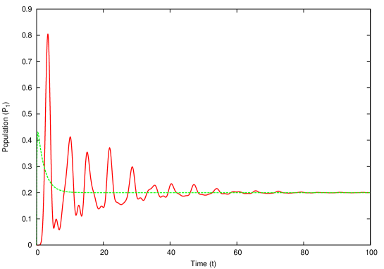
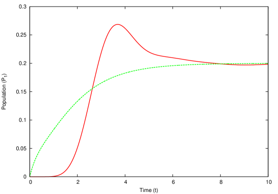
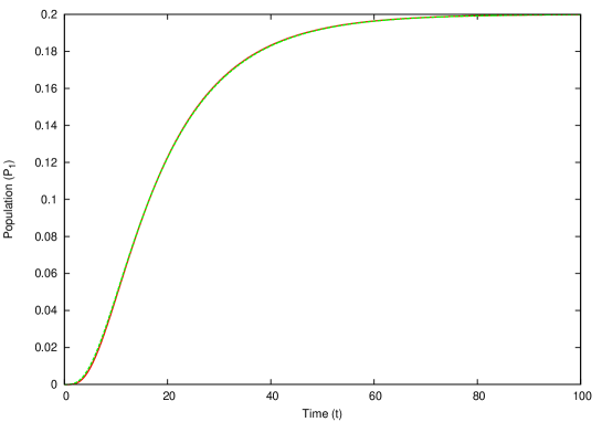
Figure 1: Time evolution of $P_{1}$ for three different values of dephasing rate: $\Gamma=0.1$ (top), $\Gamma=1.0$ (middle), and $\Gamma=10$ (bottom). The red and dashed-green lines in each panel denote results based on the original quantum dynamics (23) and the effective classical equation (24), respectively.

We next compare of the original quantum dynamics with the classical reduction. We consider the case wherein the particle is initially at site $N$. In our study, we numerically calculated the population at site 1, $P_{1}(t)=\mathrm{Tr}[n_{1}\rho(t)]$ for the system size $N=5$ and three different values of the dephasing rate $\Gamma$ (Fig. 1). In all cases, the population $P_{1}$ converges to $1/5$. However, the intermediate behaviour of the reduced equation is different from the original quantum dynamics for $\Gamma=0.1$ and $\Gamma=1$. In contrast, for the case of $\Gamma=10$, the classical and the quantum time evolutions agree with each other. This is because quantum effects decreases as the dephasing rate increases.

In the above example, we consider the quantity $n_{k}$ which does not vary under the transformation (21). The work of the transformation (21) is shown in the following section.

4 Energy Transport and RWA

In this section, we show that our formulation includes the RWA that is a standard method to study quantum open systems. By means of our method, we can clearly explain why the RWA gives unphysical results for energy transport problems.

A system in contact with heat reservoirs is frequently described by the Redfield equation bib9.0 ; bib9.2 ; bib9.3 ; bib9.4 ; bib9.5 . It is derived from the total Hamiltonian:

$$H_{\mathrm{tot}}=H_{\mathrm{S}}+\lambda H_{\mathrm{SB}}+H_{\mathrm{B}},$$ (30)

where $H_{\mathrm{S}}$, $H_{\mathrm{SB}}$, and $H_{\mathrm{B}}$ denote the system Hamiltonian, the system–bath interaction Hamiltonian, and the bath Hamiltonian respectively. The system–bath coupling $\lambda$ is assumed to be weak. Here, we assume $H_{\mathrm{SB}}$ as the following:

$$H_{\mathrm{SB}}=X\otimes Y,$$ (31)

where $X$ and $Y$ denote Hermitian operators that operate on the Hilbert space of the system and that of the bath, respectively. Utilizing the second-order perturbation with several approximations, the Redfield equation is obtained in the following form:

$$\frac{d}{dt}\rho={\cal L}^{(\mathrm{Red})}\rho=i[\rho,H_{\mathrm{S}}]+\pi\lambda^{2}\sum_{i,j}\bigl{(}\Gamma_{ij}\bra{\epsilon_{i}}X\ket{\epsilon_{j}}[\ket{\epsilon_{i}}\bra{\epsilon_{j}}\rho,X]+h.c.\bigr{)},$$ (32)

where $\ket{\epsilon_{i}}$ denotes the energy eigenstate of the eigenvalue $\epsilon_{i}$ of $H_{\mathrm{S}}$ and $\Gamma_{ij}$ denote the Fourier transformations of the reservoir correlation function. The temperature of the reservoir $\beta$ is given by the Kubo–Martin–Schwinger condition:

$$\Gamma_{ij}=\mathrm{e}^{-\beta(\epsilon_{i}-\epsilon_{j})}\Gamma_{ji}.$$ (33)

The RWA is usually carried out by considering the interaction picture, which results in the following classical master equation bib1.0 :

$$\frac{d}{dt}P_{k}(t)=2\pi\lambda^{2}\sum_{i}\bigl{(}\Gamma_{ki}|X_{ik}|^{2}P_{i}(t)-\Gamma_{ik}|X_{ik}|^{2}P_{k}(t)\bigr{)},$$ (34)

where $P_{k}(t)$ denotes the probability of observing the energy $\epsilon_{k}$ at time $t$.

It is easily verified that Eq. (34) is equivalent to time evolution by ${\cal L}^{(\mathrm{Red})}_{\mathrm{PP}}$ with the energy representation. The Redfield equation (32) is obtained by means of the second-order perturbation with respect to $\lambda$. Hence, for the same level of accuracy, the effective classical Liouvillian (17) becomes ${\cal L}_{\mathrm{eff}}\simeq{\cal L}^{(\mathrm{Red})}_{\mathrm{PP}}$. This indicates that the procedure of the RWA represented by Eq. (32) through Eq. (34) is accounted for in our formulation, and it also indicates that at the same time the observables should be transformed by Eq. (21).

As an example, let us calculate the expectation value of the energy current in the steady state for the following non-equilibrium systems:

$$\left\{\begin{array}[]{l}{\displaystyle\frac{d}{dt}\rho=i[\rho,H]+\gamma(\sigma_{1}^{-}\rho\sigma_{1}^{+}-\frac{1}{2}\{\sigma_{1}^{+}\sigma_{1}^{-},\rho\})+\gamma(\sigma_{2}^{+}\rho\sigma_{2}^{-}-\frac{1}{2}\{\sigma_{2}^{-}\sigma_{2}^{+},\rho\})}\\ H=\ket{1}\bra{2}+\ket{2}\bra{1}+h(n_{1}+n_{2}).\end{array}\right.$$ (35)

where $\sigma_{k}^{+}=\ket{k}\bra{0}$, $\sigma_{k}^{-}=\ket{0}\bra{k}$, and $\ket{0}$ denotes the vacuum state. Here we are only concerned with the single exciton space, that is, we exclude the state $\sigma_{1}^{+}\sigma_{2}^{+}\ket{0}$. Although we introduce the above quantum master equation a priori here, the RWA can be performed for weak coupling, i.e., small values of $\gamma$. The eigenvalues of the Hamiltonian are $\epsilon_{0}=0$, $\epsilon_{1}=h-1$, and $\epsilon_{2}=h+1$. The RWA can be performed if $\epsilon_{i}-\epsilon_{j}\gg\gamma\ (i\neq j)$ is satisfied, and it can be realized by assuming a suitable value of $h$. We define the energy current $J$ as

$$J=-ih(\ket{1}\bra{2}-\ket{2}\bra{1})$$ (36)

As in the case of the Redfield equation, for the purpose of simplicity, we ignore the second- and higher-order $\gamma$ terms.

We first calculate the expectation of the energy current $\langle J\rangle$ in the steady state without using the RWA. The bracket $\langle\ \rangle$ denotes the statistical average of the observables. The time derivative of an observable $A$ is given by

$$\frac{d}{dt}A={\cal L}^{\dagger}A=-i[A,H]+\gamma(\sigma_{1}^{+}A\sigma_{1}^{-}-\frac{1}{2}\{\sigma_{1}^{+}\sigma_{1}^{-}.A\})+\gamma(\sigma_{2}^{-}A\sigma_{2}^{+}-\frac{1}{2}\{\sigma_{2}^{-}\sigma_{2}^{+}.A\}).$$ (37)

Using this equation, we can write the time derivatives of the expectation values of observables by

$$\left\{\begin{array}[]{l}{\displaystyle\frac{d}{dt}\langle J\rangle=-2h(\langle n_{1}\rangle-\langle n_{2}\rangle)-\frac{\gamma}{2}\langle J\rangle}\\ {\displaystyle\frac{d}{dt}\langle n_{1}\rangle=\frac{1}{h}\langle J\rangle-\gamma\langle n_{1}\rangle}\\ {\displaystyle\frac{d}{dt}\langle n_{2}\rangle=-\frac{1}{h}\langle J\rangle+\gamma\langle n_{0}\rangle}.\end{array}\right.$$ (38)

Moreover, the completeness relation

$$\sum_{k=0}^{2}n_{k}=1$$ (39)

holds. In the steady state, the left-hand sides of the equations (38) vanish. Solving Eqs. (38) and (39), we obtain the expectation value of the energy current in the steady state:

$$\langle J\rangle\simeq\frac{\gamma h}{3},$$ (40)

where the higher order of $\gamma$ has been omitted.

Next, we compute the energy current $J$ with the RWA. The RWA results in the classical Liouvillian:

$${\cal L}_{\mathrm{eff}}=\frac{\gamma}{2}\begin{pmatrix}-2&1&1\\ 1&-1&0\\ 1&0&-1\end{pmatrix},$$ (41)

where the basis $\{\ket{\epsilon_{0}}\bra{\epsilon_{0}},\ket{\epsilon_{1}}\bra{\epsilon_{1}},\ket{\epsilon_{2}}\bra{\epsilon_{2}}\}$ is used in this order. The steady-state solution of the Liouvillian (41) is given as

$$\rho^{\mathrm{ss}}=\frac{1}{3}(\ket{\epsilon_{0}}\bra{\epsilon_{0}}+\ket{\epsilon_{1}}\bra{\epsilon_{1}}+\ket{\epsilon_{2}}\bra{\epsilon_{2}}).$$ (42)

The energy current is expressed in the energy basis as

$$J=ih(\ket{\epsilon_{1}}\bra{\epsilon_{2}}-\ket{\epsilon_{2}}\bra{\epsilon_{1}}).$$ (43)

We note that the expression for $J$ has no P-space components. In conventional approaches, the energy current $J$ is used without any changes, thereby resulting in $\mathrm{Tr}[J\rho^{\mathrm{ss}}]=0$. This brings to light the necessity of the transformation of $J$ to $\tilde{J}$. From Eqs. (21) and (37), the transformed current $\tilde{J}$ is given as

$$\tilde{J}\simeq J+\frac{\gamma h}{4}(2\ket{\epsilon_{0}}\bra{\epsilon_{0}}+\ket{\epsilon_{1}}\bra{\epsilon_{1}}+\ket{\epsilon_{2}}\bra{\epsilon_{2}}),$$ (44)

which reproduces the correct expectation value of the energy current

$$\langle\tilde{J}\rangle=\mathrm{Tr}[\tilde{J}\rho^{\mathrm{ss}}]=\frac{\gamma h}{3}.$$ (45)

5 Exact Replacement with Classical Dynamics

The reduced equation (17) is derived by expanding the original quantum master equation with respect to $1/\Gamma$. Therefore, it is only valid for large values of $\Gamma$. In this section, we show that the replacement of quantum dynamics with the classical equation can be carried out for any values of the parameters for quantities such as transport efficiency.

Let us consider the quantum open system that is described by the Markovian quantum master equation:

$$\frac{d}{dt}\rho={\cal L}\rho.$$ (46)

Let us assume that the quantum master equation has a unique steady state $\rho^{\mathrm{ss}}$. Let us consider the following quantity:

$$\zeta=\int^{\infty}_{0}dt\mathrm{Tr}[A\mathrm{e}^{{\cal L}t}\rho(0)],$$ (47)

where $A$ denotes a P-space observable that satisfies $\mathrm{Tr}[A\rho^{\mathrm{ss}}]=0$.

We first show that the time integral in Eq. (47) is related to a certain steady-state problem from the analogy of the linear-response theory. For this purpose, we modify the Liouvillian ${\cal L}$ to ${\cal K}$ as

$${\cal K}={\cal L}+\epsilon\chi,$$ (48)

where $\epsilon$ is the small parameter and the superoperator $\chi$ satisfies

$$\chi={\cal P}\chi{\cal P},\ \ \chi\rho^{\mathrm{ss}}=\chi\rho_{\mathrm{P}}^{\mathrm{ss}}=\rho(0),$$ (49)

where $\rho_{\mathrm{P}}^{\mathrm{ss}}$ denotes the P-space components of $\rho^{\mathrm{ss}}$. The steady-state solution $\eta$ of the modified Liouvillian ${\cal K}$ is expressed as

$$\eta=\rho^{\mathrm{ss}}+\epsilon\int^{\infty}_{0}dt\mathrm{e}^{{\cal L}t}\chi\rho^{\mathrm{ss}}+{\cal O}(\epsilon^{2})=\rho^{\mathrm{ss}}+\epsilon\int^{\infty}_{0}dt\mathrm{e}^{{\cal L}t}\rho(0)+{\cal O}(\epsilon^{2}).$$ (50)

Thus, $\zeta$ can be represented as

$$\zeta=\lim_{\epsilon\to 0}\epsilon^{-1}\mathrm{Tr}[A\eta]=\lim_{\epsilon\to 0}\epsilon^{-1}\mathrm{Tr}[A\eta_{\mathrm{P}}],$$ (51)

where $\eta_{\mathrm{P}}$ represents the P-space components of $\eta$.

The steady-state problem is expressed as

$$\begin{pmatrix}{\cal L}_{\mathrm{PP}}+\epsilon\chi&{\cal L}_{\mathrm{PC}}\\ {\cal L}_{\mathrm{CP}}&{\cal L}_{\mathrm{CC}}\end{pmatrix}\begin{pmatrix}\eta_{\mathrm{P}}\\ \eta_{\mathrm{C}}\end{pmatrix}=0.$$ (52)

Let us transform the above equation by the superoperator ${\cal S}$

$${}{\cal S}=\begin{pmatrix}I&0\\ {\cal L}_{\mathrm{CC}}^{-1}{\cal L}_{\mathrm{CP}}&I\end{pmatrix}.$$ (53)

From Eqs. (7) and (8), we obtain the following equation:

$${\cal S}{\cal L}{\cal S}^{-1}{\cal S}\eta=\begin{pmatrix}{\cal L}_{\mathrm{eff}}+\epsilon\chi&{\cal L}_{\mathrm{PC}}\\ {\cal L}_{\mathrm{CC}}^{-1}{\cal L}_{\mathrm{CP}}({\cal L}_{\mathrm{eff}}+\epsilon\chi)&{\cal L}_{\mathrm{CC}}^{-1}{\cal L}_{\mathrm{CP}}{\cal L}_{\mathrm{PC}}+{\cal L}_{\mathrm{CC}}\end{pmatrix}\begin{pmatrix}\eta_{\mathrm{P}}\\ 0\end{pmatrix}=0.$$ (54)

Thus, $\eta_{\mathrm{P}}$ is the steady-state solution of the superoperator ${\cal L}_{\mathrm{eff}}+\epsilon\chi$, and it can be expressed as

$$\eta_{P}=\rho_{\mathrm{P}}^{\mathrm{ss}}+\epsilon\int^{\infty}_{0}dt\mathrm{e}^{{\cal L}_{\mathrm{eff}}t}\rho(0)+{\cal O}(\epsilon^{2}).$$ (55)

Using Eqs. (50), (51), and (55), we obtain the following equation:

$$\zeta=\int^{\infty}_{0}dt\mathrm{Tr}[A\mathrm{e}^{{\cal L}t}\rho(0)]=\int^{\infty}_{0}dt\mathrm{Tr}[A\mathrm{e}^{{\cal L}_{\mathrm{eff}}t}\rho(0)].$$ (56)

Thus, the time evolution of the quantum system is fully replaced by population dynamics.

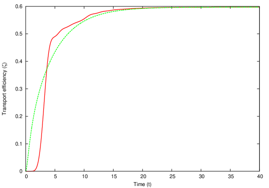
Figure 2: Numerical calculation of $\zeta(t)$ based on the original quantum dynamics (red line) and the classical dynamics (green dashed-line). The original quantum evolution asymptotically coincides with the classical replacement in the long-time regime.

To validate the above argument, we numerically calculate the quantum transport efficiency for the system given by the following equation:

$$\frac{d}{dt}\rho={\cal L}\rho=i[\rho,H]+{\cal L}_{\mathrm{deph}}\rho+{\cal L}_{\mathrm{diss}}\rho+{\cal L}_{\mathrm{trap}}\rho,$$ (57)

where the Hamiltonian $H$ is the tight-binding model given by Eq. (22), and the Lindblad superoperators are given by

$$\left\{\begin{array}[]{l}{\cal L}_{\mathrm{deph}}=\gamma{\displaystyle\sum_{k=1}^{N}(n_{k}\rho n_{k}-\frac{1}{2}\{n_{k},\rho\})}\\ {\cal L}_{\mathrm{diss}}={\displaystyle\mu\sum_{k=1}^{N}(\sigma_{k}^{-}\rho\sigma_{k}^{+}-\frac{1}{2}\{\sigma_{k}^{+}\sigma_{k}^{-},\rho\})}\\ {\cal L}_{\mathrm{trap}}=\kappa(\sigma_{1}^{-}\rho\sigma_{1}^{+}-\frac{1}{2}\{\sigma_{1}^{+}\sigma_{1}^{-},\rho\}).\\ \end{array}\right.$$ (58)

The raising and lowering operators at the $k$-th site are denoted by $\sigma_{k}^{+}$ and $\sigma_{k}^{-}$, respectively. Let us suppose that the particle is at the $N$-th site initially. The transport efficiency is defined by how often the particle is trapped at the first site during the time interval $t$, which efficiency is expressed by

$$\zeta(t)=\kappa\int^{t}_{0}ds\mathrm{Tr}[n_{1}\mathrm{e}^{{\cal L}s}\rho(0)],$$ (59)

where $\zeta(t)$ represents the transport efficiency at time $t$. We numerically calculate the time evolution of $\zeta(t)$ with parameters $N=5$, $\kappa=1$, $\mu=0.1$, and $\gamma=0.1$ (Fig. 2). The classical time evolution based on the Liouvillian ${\cal L}_{\mathrm{eff}}$ does not coincide with the original quantum time evolution in the short-time regime; however, the time evolutions converge with the same value in the long-time regime.

We note that the superoperator ${\cal L}_{\mathrm{eff}}$ does not ensure the positivity of the density matrix in general. Nevertheless, in the case of the transport efficiency problem, the time evolution can be intuitively interpreted. This is because the superoperator ${\cal L}_{\mathrm{eff}}$ is trace-preserving. Therefore, the particle flow can be defined. The only difference with respect to the general classical picture is that negative values of population can be obtained.

6 Conclusions

We have proposed a general method to reduce a quantum master equation to a classical one by utilizing a similarity transformation. Our formulation reveals the necessity of the transformation of observables. This is the solution of the problem that the energy flow through the system vanishes in the RWA scheme. We have also shown that the exact replacement with classical dynamics is possible for the calculation of a quantity such as the transport efficiency. Our method facilitates an understanding of several mechanisms of environment-assisted quantum transport in the unified picture prepare .

The introduction of a similarity transformation is also observed in the study of the non-relativistic reduction of the Dirac equation with electromagnetic fields bib10.0 ; bib10.1 . In such a case, the transformation is performed on the Hamiltonian, and hence, it should be a unitary transformation. However, the nature of the similarity transformation in the Liouville space has not been understood clearly. Thus, it is important to examine as to what kinds of transformations conserve the nature of the Liouvillian that is of the Lindblad form.

The argument in this paper is general, and therefore, we expect that the results can be applied to a wide range of quantum physics problems.

References

- (1) H-P. Breuer and F. Petruccione, The Theory of Open Quantum Systems (Oxford University Press, Oxford, 2002)
- (2) S. Hoyer, M. Sarovar, and K. B. Whaley, New J. Phys. 12, 065041 (2010)
- (3) H. Haken and P. Reineker, Z. Phys. 249, 253 (1972)
- (4) G. Lindblad, Commun. Math. Phys. 48, 119 (1976)
- (5) H. Wichterich, M. J. Henrich, H-P. Breuer, J. Gemmer, and M. Michel, Phys. Rev. E 76, 031115 (2007)
- (6) M. Esposito, U. Harbola, and S. Mukamel, Rev. Mod. Phys. 81, 1665 (2009)
- (7) T. Yuge, T. Sagawa, A. Sugita, and H. Hayakawa, Phys. Rev. B 86, 235308 (2012)
- (8) K. Saito, S. Takesue, and S. Miyashita, Phys. Rev. E 61, 2397 (2000)
- (9) T. Prosen and B. Žunkovič, New J. Phys. 12, 025016 (2010)
- (10) J. Wu and M. Berciu, Phys. Rev. E 83, 214416 (2011)
- (11) M. Michel and O. Hess, Phys. Rev. B. 77, 104303 (2008)
- (12) K. Saito, Europhys Lett. 61, 34 (2003)
- (13) M. Znidaric, T. Prosen, G. Benetti, G. casati, and D. Rossini, Phys. Rev. E. 81, 051135 (2010)
- (14) T. Prosen, New J. Phys. 10, 043026 (2008)
- (15) R. Steinigeweg, M. Ogiewa, and J. Gemmer, EPL 87, 10002 (2009)
- (16) K. Sun, C. Wang, and Q. Chen, EPL 92, 24002 (2010)
- (17) W. Li and P. Tong, Phys. Rev. E 83, 031128 (2011)
- (18) Y. Yan, C.-Q. Wu, G. Casati, T. Prosen, and B. Li, Phys. Rev. B 77, 172411 (2008)
- (19) S. Attal and Y. Pautrar, Ann. Henri Poincaré 7, 59 (2006)
- (20) A. Dhahri, J. Phys. A 41, 275305 (2008)
- (21) M. B. Plenio and S. F. Huelga, New J. Phys. 10, 113019 (2008)
- (22) P. Rebentrost, M. Mohseni, I. Kassal, S. Lloyd, and A. Aspuru-Guzik, New J. Phys. 11, 033003 (2009)
- (23) I. Kassal and A. Aspuru-Guzik, New J. Phys. 14, 053041 (2012)
- (24) K. M. Pelzer, A. F. Fidler, G. B. Griffin, S. K. Gray, and G. S. Engel, New J. Phys. 15, 095019 (2013)
- (25) N. Kamiya and S. Takesue, J. Phys. Soc. Jpn. 82, 114002 (2013)
- (26) M. Žnidarič, New J. Phys. 12, 043001 (2010)
- (27) M. Žnidarič, J. Stat. Mech. 2010, L05002 (2010)
- (28) D. Manzano, M. Tiersch, A. Asadian, and H. J. Briegel, Phys. Rev. E 86, 061118 (2012)
- (29) J. J. Mendoza-Arenas, T. Grujic, D. Jaksch, and S. R. Clark, Phys. Rev. E 87, 235130 (2013)
- (30) in preparation.
- (31) L. L. Foldy and S. A. Wouthuysen, Phys. Rev. 78, 29 (1950)
- (32) S. Okubo, Prog. Theor. Phys. 12, 603 (1954)