Linearized fluid/gravity correspondence: from shear viscosity to all order hydrodynamics

Abstract

In ref. 1406.7222 , we reported a construction of all order linearized fluid dynamics with strongly coupled $\mathcal{N}=4$ super-Yang-Mills theory as underlying microscopic description. The linearized fluid/gravity correspondence makes it possible to resum all order derivative terms in the fluid stress tensor. Dissipative effects are fully encoded by the shear term and a new one, emerging starting from third order in hydrodynamic derivative expansion. In this work, we provide all computational details omitted in 1406.7222 and present additional results. We derive closed-form linear holographic RG flow-type equations for momenta-dependent transport coefficient functions. Generalized Navier-Stokes equations are shown to emerge from the constraint components of the bulk Einstein equations. We perturbatively solve the RG equations for the viscosity functions, up to third order in derivative expansion, and up to this order compute spectrum of small fluctuations. Finally, we solve the RG equations numerically, thus accounting for all order derivative terms in the boundary stress tensor.

1 Introduction

In heavy ion collisions at RHIC and LHC, a novel state of QCD matter, quark-gluon plasma, is created. The quark-gluon plasma produced at RHIC was discovered to behave like a nearly perfect fluid reflecting strongly coupled regime of QCD nucl-th/0405013 ; hep-ph/0405066 , with relativistic hydrodynamics found to provide an accurate description of the plasma fireball expansion. The hydrodynamic evolution of the quark-gluon plasma is characterized by a set of transport coefficients, which have to be computed from the microscopic QCD. However, strongly coupled nature of this system prevents from a first principe analytic calculation of these coefficients. While lattice methods are quite reliable in studying QCD thermodynamics hep-lat/0611014 ; 1007.2580 ; 1309.5258 , they usually fail in extracting transport coefficients due to limited applicability to real-time dynamics. Therefore, various microscopic models are indispensable to understand transport properties of this QCD matter.

Fluid dynamics fluid1 ; fluid2 is an effective description of most interacting quantum field theories at long wavelengths. The description is of statistical nature: it captures collective dynamics of a large number of microscopic degrees of freedom. The collective variables suitable for such a description are local densities of conserved charges, local fluid velocity and temperature. Hydrodynamic equations are local conservation laws for corresponding currents, which are specified via constitutive relations. As a low energy effective field theory, fluid dynamics describes near-thermal equilibrium systems and is naturally defined in terms of derivative expansion of the local fluid mechanical variables. Up to a finite number of transport coefficients, the derivative expansion at any given order is completely fixed by thermodynamic and symmetry considerations. Transport coefficients, such as viscosities and conductivities, must be determined from either experimental measurements or theoretical computations in the underlying microscopic theory.

The stress tensor $T_{\mu\nu}$ of a relativistic fluid is usually presented as a sum of two terms

$$T_{\mu\nu}=T_{\mu\nu}^{\text{Ideal}}+T_{\mu\nu}^{\text{Diss}},$$ (1)

where $T_{\mu\nu}^{\text{Ideal}}$ corresponds to ideal fluid dynamics and for conformal fluids has the form

$$T_{\mu\nu}^{\text{Ideal}}=\frac{1}{{\bf b}^{4}}(\eta_{\mu\nu}+4u_{\mu}u_{\nu}),$$ (2)

where $\eta_{\mu\nu}$ is the four dimensional Minkowski metric, the fluid’s four velocity is $u_{\mu}$ and, in our notations, the temperature is

$$T=\frac{1}{\pi\bf b}.$$ (3)

$T_{\mu\nu}^{\text{Diss}}$ accounts for dissipative effects and is chosen to be nonzero only for spatial components. Up to the first velocity gradient it is given by the Navier-Stokes term

$$T_{ij}^{\text{Diss}}=-\eta_{0}\,\sigma_{ij},$$ (4)

where $\eta_{0}$ is the shear viscosity coefficient and the tensor $\sigma_{ij}$ has the form

$$\sigma_{ij}=\frac{1}{2}\left(\partial_{i}\beta_{j}+\partial_{j}\beta_{i}-\frac{2}{3}\delta_{ij}\partial\beta\right),~{}~{}~{}~{}~{}~{}~{}~{}~{}u_{i}=\frac{\beta_{i}}{\sqrt{1-\beta^{2}}}.$$ (5)

Theoretical foundations of relativistic dissipative fluid dynamics are not yet fully established. The relativistic Navier-Stokes equations are a-causal and unstable instable1 ; instable2 ; instable3 ; instable4 : the irreversible currents are linearly proportional to the thermodynamic forces, which have instantaneous influence on the currents, obviously violating causality. These problems can be solved by introducing retardation into the definitions of the irreversible currents IS1 ; IS2 , leading to equations of motion for these currents, which thus become independent dynamical variables. Theories of this type are known as causal relativistic dissipative fluid dynamics. Causality usually also implies stability 0907.3906 . To obtain a causal formulation, one needs to include higher order terms in the gradient expansion of the currents, in which case additional transport coefficients arise. Truncation at any fixed order would presumably lead to violation of causality that can be fully restored only at infinite order, which we refer to as an all-order gradient resummation. Non-trivial physical consequences imposed by causality of relativistic fluids were investigated in instable1 ; instable2 ; instable3 ; instable4 ; 0807.3120 ; 0907.3906 ; 1102.4780 and lead to certain constraints on possible values of higher order transport coefficients.

AdS/CFT correspondence hep-th/9711200 ; hep-th/9802109 ; hep-th/9802150 ; hep-th/9905111 emerged over a decade ago as a standard tool and a model playground for addressing strongly coupled dynamics of gauge theories. The AdS/CFT correspondence relates holographically a large $N$ strongly interacting quantum field theory with dynamics of classical gravity in (asymptotically) AdS spacetime. Fluid/gravity correspondence hep-th/0104066 ; hep-th/0205052 ; hep-th/0405231 ; hep-th/0512162 is a long wavelength limit of the AdS/CFT correspondence: it gives a map between black holes in asymptotically AdS spacetime and fluid dynamics of a strongly coupled boundary field theory. The most celebrated prediction of the fluid/gravity correspondence is a ratio of the shear viscosity $\eta_{0}$ to the entropy density $s$ hep-th/0104066 ; hep-th/0205052 ; hep-th/0405231 ,

$$\frac{\eta_{0}}{s}=\frac{1}{4\pi}.$$ (6)

The ratio (6) is universal for a large class of strongly coupled gauge theory plasmas for which holographic duals are governed by Einstein gravities in asymptotically AdS spacetimes. Remarkably, this small ratio is quite close to the values extracted for QCD plasma from the RHIC experiments. Universality of this ratio was further proved in hep-th/0311175 ; 0808.1837 and in 0809.3808 using black hole membrane paradigm. It was later found that university of the ratio (6) gets violated by either modifying Einstein gravity 0712.0743 ; 0712.0805 ; 0806.2156 ; 0812.2521 ; 0811.1665 ; 0901.1421 ; 0903.2527 ; 0903.2834 ; 0903.3244 ; 0908.1473 or breaking isotropic invariance among spatial directions 1011.5912 ; 1109.4592 ; 1110.6825 ; 1406.6019 . We refer the reader to 0704.0240 for a comprehensive review on early literature.

A specific realization of the fluid/gravity correspondence, and the one we will closely follow below, was established in 0712.2456 : it provides a systematic framework to construct a universal nonlinear fluid dynamics, order by order in the boundary derivative expansion. The stress tensor for the dual conformal fluid was explicitly constructed in 0712.2456 up to second order in derivative expansion, which is in perfect agreement with a general form of second order conformal hydrodynamics as analyzed in 0712.2451 . Computations of 0712.2456 were later generalized to conformal fluids in flat 0806.4602 and also weakly curved 0809.4272 background manifolds of various dimensions. Forced fluids in a weakly curved manifold were examined in 0806.0006 by studying long wavelength solutions of Einstein-dilaton gravity with negative cosmological constant. Further developments can be found in reviews 0905.4352 ; 1107.5780 and references therein.

Refs. 0704.1647 ; 0905.4069 (see also 1103.3452 ; 1203.0755 ; 1302.0697 ) initiated study of generalized relativistic hydrodynamics by considering all orders in derivatives of local fluid mechanical variables in the stress tensor.

All order or resummed hydrodynamics is found to accommodate certain contributions, which are not present in a strict low momentum approximation. To avoid any confusion we thus clarify the terminology: by hydrodynamics we mean an effective theory given by a constitutive relation for the stress tensor in terms of temperature, fluid velocity and their gradients only. Navier-Stokes or any “unresummed” hydrodynamics involves only a finite number of gradients, while all order or “resummed” hydrodynamics means infinite number of gradients, but no other degrees of freedom.

The higher order derivative expansion generally includes two types of terms: nonlinear in the fluid velocity, like $(\nabla u)^{2}$, and linear ones like $\nabla\cdots\nabla u$. The nonlinearities are significant when amplitudes of local fluid mechanical variables are large. However, even for fluid perturbations with small amplitudes, one can get large contributions from the linear terms when the momenta associated with the fluid perturbations are large. Given that these two types of terms are controlled by different parameters, it is possible to separate these contributions and to have the linear terms under theoretical control. We will focus on those linear terms in the rest of this paper.

To collect all order linear terms in a self-consistent manner, the shear viscosity $\eta_{0}$ was generalized into momenta-dependent function $\eta(\omega,q^{2})$. This viscosity function is expressed in momentum space which follows from the replacement $\partial_{\mu}\to\left(-i\omega,i\vec{q}\right)$ in the linear gradient expansion of $T_{\mu\nu}$. By postulating a constitutive relation for $T_{\mu\nu}$ in terms of the shear viscosity function $\eta(\omega,q^{2})$, the authors of 0905.4069 attempted to extract $\eta(\omega,q^{2})$ from thermal correlators of the stress tensor computed on the gravity side hep-th/0205051 ; hep-th/0602059 . While certain progress was achieved in 0905.4069 , its prime goal of complete determination of the viscosity function was not reached. It was realized that even in the case of linearized hydrodynamics, knowledge of retarded correlators contains insufficient information about all transport properties of the system. In ref. 1406.7222 , we succeeded to completely solve this problem and below we provide all the details related to our computations.

In ref. 1406.7222 , we reported progress, achieved via linearizing fluid/gravity correspondence, in consistently generalizing relativistic hydrodynamics to all orders. Upon linearization, perturbative computations of 0712.2456 can be straightforwardly extended to arbitrary order in the boundary derivative expansion. Our procedure is, however, slightly different from that of 0712.2456 . Particularly, the dissipative part in the stress tensor is collected in a unified way, rather than being determined order by order in derivative expansion. The Einstein equations in the bulk are split into two sets: dynamical equations and constraints. It turns out that in order to derive transport coefficient functions, it is sufficient to solve dynamical components of the bulk Einstein equations only. By solving only those we construct an “off-shell” fluid stress tensor. The remaining constraint components of the Einstein equations are equivalent to conservation laws of thus constructed fluid stress tensor and lead to generalized Navier-Stokes equations. It is worth emphasizing that the bulk dynamics is not absorptive, rather the bulk acts as a non-linear dispersive medium. Dissipative effects emerge via absorptive boundary conditions at the black hole horizon.

We find that the dissipative part of the stress tensor has the following form

$$T_{ij}^{\text{Diss}}=-\left[\eta(\omega,q^{2})\sigma_{ij}+\zeta(\omega,q^{2})\pi_{ij}\right],$$ (7)

where $\pi_{ij}$ is a third order tensor structure

$$\pi_{ij}=\partial_{i}\partial_{j}\partial\beta-\frac{1}{3}\delta_{ij}\partial^{2}\partial\beta$$ (8)

and $\zeta(\omega,q^{2})$ is a new viscosity function, which in 0905.4069 , apparently incorrectly, was argued to be zero. We here express the viscosity functions in momentum space but with tensors $\sigma_{ij}$ and $\pi_{ij}$ formulated as explicit derivatives of the fluid velocity. Later, the notations $\eta(\partial_{v},\partial^{2})$ and $\zeta(\partial_{v},\partial^{2})$ will also be used to denote the viscosity functions. All these expressions are interchangeable under the above rule of replacement. We will be working using dimensionless units for all the momenta, choosing units such that the temperature is normalized to $\pi T=1$. So all the physical momenta should be understood as in units of $\pi\,T$: $\omega\pi T$ and $q_{i}\pi T$.

In the hydrodynamic limit $\omega,q_{i}\ll 1$, $\eta(\omega,q^{2})$ and $\zeta(\omega,q^{2})$ are expandable in power series and a perturbative analysis to be presented below reveals a few first terms in the expansions,

$$\begin{split}\eta(\omega,q^{2})&=2+(2-\ln{2})i\omega-\frac{1}{4}q^{2}-\frac{1}{24}\left[6\pi-\pi^{2}+12\left(2-3\ln{2}+\ln^{2}{2}\right)\right]\omega^{2}+\cdots,\\ \zeta(\omega,q^{2})&=\frac{1}{12}\left(5-\pi-2\ln{2}\right)+\cdots,\end{split}$$ (9)

where in our units, the first term in $\eta$ corresponds to the ratio (6), while the second term accounts for the relaxation time hep-th/0703243 ; 0712.2451 ; 0712.2456 ; 0712.2916 ; 0811.1794 . The remaining two terms in equation (9) are new third order transport coefficients. In section 4, $\eta(\omega,q^{2})$ and $\zeta(\omega,q^{2})$ are computed numerically to all orders, and we will also present expansions of these viscosity functions up to fifth order.

The remaining part of this paper is organized as follows. In section 2, we outline the derivation of the fluid dynamics from the bulk gravity. The main results are formulated as closed linear holographic RG flow-type equations for the generalized transport coefficient functions and generalized Navier-Stokes equations. We then compute dispersion relations for sound and shear modes. In section 3, to make comparison with previous studies in the literature, we perturbatively solve these holographic RG flow-type equations and obtain the fluid stress tensor up to third order in the derivative expansion. In section 4, we numerically solve the RG flow-type equations and obtain generalized transport coefficient functions, extending the perturbative analysis of section 3 to very large momenta. We also extract the viscosity functions via an approximate matching scheme, and find perfect agreement with the numerical results. Summary and discussion can be found in section 5.

2 Fluid dynamics from the bulk gravity

2.1 Linearized fluid/gravity correspondence

The fluid/gravity correspondence makes it possible to construct the fluid stress tensor and prove its conservation law (Navier-Stokes equations) by solving the bulk Einstein equations in asymptotically AdS spacetime, in the long wavelength limit. We start by considering a universal sector of the AdS/CFT correspondence: classical Einstein gravity with a negative cosmological constant in five dimensional spacetime,

$$S=\frac{1}{16\pi G_{N}}\int d^{5}x\sqrt{-g}\left(R+12\right),$$ (10)

where the AdS radius is set to one for convenience. The Einstein equations which follow from the action (10) are

$$E_{MN}\equiv R_{MN}-\frac{1}{2}g_{MN}R-6g_{MN}=0.$$ (11)

We use upper case Latin indices $\{M,N,\cdots\}$ and lower case Greek indices $\{\mu,\nu,\cdots\}$ to denote bulk and boundary directions, respectively. Lower case Latin indices $\{i,j,\cdots\}$ will be used to specify spatial directions along the boundary.

Besides pure $AdS_{5}$ spacetime which is dual to the vacuum state of the boundary CFT, the action (10) also admits a 4-parameter family of Black Hole solutions,

$$ds^{2}=-2u_{\mu}dx^{\mu}dr-r^{2}f\left({\bf b}r\right)u_{\mu}u_{\nu}dx^{\mu}dx^{\nu}+r^{2}\mathcal{P}_{\mu\nu}dx^{\mu}dx^{\nu},$$ (12)

with

$$u_{v}=-\frac{1}{\sqrt{1-\beta^{2}}},~{}~{}~{}~{}u_{i}=\frac{\beta_{i}}{\sqrt{1-\beta^{2}}},~{}~{}~{}~{}\beta^{2}=\sum_{i=1}^{3}\beta_{i}\beta_{i},$$ (13)

and $f(r)=1-1/r^{4}$. Hawking temperature of this black hole is

$$T=\frac{1}{\pi\bf b}$$ (14)

which is identified as the temperature of the dual CFT. The operator $\mathcal{P}_{\mu\nu}=\eta_{\mu\nu}+u_{\mu}u_{\nu}$ acts as a projector onto spatial directions. Notice that so far the parameters $\beta_{i}$ and $\bf b$ are held constant, so that the line element (12) does form a class of solutions to the Einstein equations (11). As pointed out in 0712.2456 , the line element (12) defines a metric of a uniform black brane written in the ingoing Eddington-Finkelstein coordinate, moving at velocity $\beta_{i}$ along spatial direction $x_{i}$.

Discussing fluid dynamics we closely follow 0712.2456 and promote the constant parameters $\beta_{i}$ and $\bf b$ into arbitrarily slowly varying functions of boundary coordinates $x^{\alpha}$,

$$ds^{2}=-2u_{\mu}(x^{\alpha})dx^{\mu}dr-r^{2}f\left({\bf b}(x^{\alpha})r\right)u_{\mu}(x^{\alpha})u_{\nu}(x^{\alpha})dx^{\mu}dx^{\nu}+r^{2}\mathcal{P}_{\mu\nu}(x^{\alpha})dx^{\mu}dx^{\nu},$$ (15)

In general, (15) no longer solves the Einstein equations (11). The method developed in 0712.2456 is to add suitable corrections to (15), so that (11) is satisfied by the new line element. The corrected metric is not easily found for a general configuration. The authors of 0712.2456 introduced a systematic way to construct the corrected metric, expanding in the long wavelength limit. A scale associated with this expansion should be much larger than a characteristic scale of the system, such as inverse of the temperature $1/T$. That is the velocity and temperature fields are assumed to vary slowly on this scale, admitting a gradient expansion around some arbitrarily chosen point, such as spacetime origin $x^{\alpha}=0$. The Einstein equations (11) for the metric are then solved order by order in the boundary derivative expansion. As has been pointed out in the Introduction, the dual metric was constructed up to second order in the velocity gradient, including nonlinear terms quadratic in the velocity gradient.

Our main goal is to perform a summation over all higher order derivative terms in the boundary stress tensor, but as stressed employing linear approximation. Rather than resorting to order by order derivative expansion of 0712.2456 , we instead linearize the problem in perturbations of the fluid mechanical variables $u_{\mu}(x^{\alpha})$ and ${\bf b}(x^{\alpha})$. More specifically, the fluid velocity and temperature parameters are expanded as

$$u_{\mu}(x^{\alpha})=\left(-1,\epsilon\beta_{i}(x^{\alpha})\right)+\mathcal{O}(\epsilon^{2}),~{}~{}~{}{\bf b}(x^{\alpha})={\bf b}_{0}+\epsilon{\bf b}_{1}(x^{\alpha})+\mathcal{O}(\epsilon^{2}),$$ (16)

where, as in 0712.2456 , we multiply $\beta_{i}(x^{\alpha})$ and ${\bf b}_{1}(x^{\alpha})$ by a small number $\epsilon$, which is an order counting parameter. Below we are going to systematically trace only the terms linear in $\epsilon$ and set $\epsilon$ to one in the final expression of the fluid stress tensor. ${\bf b}_{0}$ corresponds to the equilibrium temperature of the dual fluid system while ${\bf b}_{1}(x^{\alpha})$ accounts for the dissipative corrections. In what follows, we use conformal symmetry to set ${\bf b}_{0}$ to one.

Substituting (16) into (12), the “seed” metric, i.e., a linearized version of (15) is

$$\begin{split}ds^{2}=&2drdv-r^{2}f(r)dv^{2}+r^{2}d{\vec{x}}^{2}\\ &-\epsilon\left[2\beta_{i}(x^{\alpha})drdx^{i}+\frac{2}{r^{2}}\beta_{i}(x^{\alpha})dvdx^{i}+\frac{4}{r^{2}}{\bf b}_{1}(x^{\alpha})dv^{2}\right]+\mathcal{O}(\epsilon^{2}),\end{split}$$ (17)

where the first line is the line element of $AdS_{5}$ black hole written in the ingoing Eddington-Finkelstein coordinate. As has been explained above, the metric (17) does not solve the Einstein equations (11) at order $\epsilon$. The term linear in $\epsilon$ in  (17) is only a part of the metric we are after, and additional corrections at this order have to be introduced. The full metric is formally written as

$$g=g^{(0)}+\epsilon g^{(1)}+\mathcal{O}(\epsilon^{2}),~{}~{}~{}\text{with}~{}~{}~{}g^{(1)}=g_{\text{in}}^{(1)}+g_{\text{corr}}^{(1)},$$ (18)

where $g^{(0)}$ is the first line of (17) and $g_{\text{in}}^{(1)}$ corresponds to the term linear in $\epsilon$ of (17). The term $g_{\text{corr}}^{(1)}$ is the added correction, whose form has to be determined via solving the bulk Einstein equations (11).

In order to proceed with the computations, we fix gauge. Following 0712.2456 , we work in the “background field” gauge,

$$g_{rr}=0,~{}~{}~{}g_{r\mu}\propto u_{\mu},~{}~{}~{}\textrm{Tr}\left[(g^{(0)})^{-1}g^{(1)}\right]=0.$$ (19)

We pause to explain the results of the above gauge condition. The most general form of the undetermined metric correction $g_{\text{corr}}^{(1)}$ could be parameterized as,

$$ds_{\text{corr}}^{2}=\epsilon\left(\mathfrak{g}_{rr}dr^{2}+2\mathfrak{g}_{rv}drdv+2\mathfrak{g}_{ri}drdx^{i}+\mathfrak{g}_{vv}dv^{2}+2\mathfrak{g}_{vi}dvdx^{i}+\mathfrak{g}_{ij}dx^{i}dx^{j}\right).$$ (20)

The condition $g_{rr}=0$ implies $\mathfrak{g}_{rr}=0$. The metric components $g_{r\mu}$ can be read off from eqs. (17) and (20),

$$g_{r\mu}=\left(1,-\epsilon\beta_{i}\right)+\epsilon\left(\mathfrak{g}_{rv},\mathfrak{g}_{ri}\right).$$ (21)

Therefore, the second condition $g_{r\mu}\propto u_{\mu}$ amounts to requiring that

$$\left(\mathfrak{g}_{rv},\mathfrak{g}_{ri}\right)\propto(1,-\epsilon\beta_{i})~{}\Longrightarrow\mathfrak{g}_{ri}=-\epsilon\beta_{i}\mathfrak{g}_{rv}.$$ (22)

In other words, up to $\mathcal{O}(\epsilon)$, the vector component $\mathfrak{g}_{ri}$ will be set to zero. The last condition in (19) gives a constraint,

$$\mathfrak{g}_{rv}+\frac{1}{2r^{2}}\sum_{i=1}^{3}\mathfrak{g}_{ii}=0.$$ (23)

Under the gauge condition (19), the line element (20) for $g_{\text{corr}}^{(1)}$ can be rewritten in the similar fashion as that of 0712.2456 ,

$$ds_{\text{corr}}^{2}=\epsilon\left(-3hdrdv+\frac{k}{r^{2}}dv^{2}+r^{2}hd{\vec{x}}^{2}+\frac{2}{r^{2}}j_{i}dvdx^{i}+r^{2}\alpha_{ij}dx^{i}dx^{j}\right),$$ (24)

where the trace part of $\mathfrak{g}_{ij}$ is explicitly denoted as scalar function $h$. Therefore, $\alpha_{ij}$ is a symmetric traceless tensor of rank two. Notice that all the metric components $\{h,~{}k,~{}j_{i},~{}\alpha_{ij}\}$ are functions of the bulk coordinates $\{x^{\alpha},r\}$. We shall find that these functions are functionals of the fluid velocity $\beta_{i}$, which we leave as an undetermined parameter. Their precise forms have to be determined by solving the bulk Einstein equations (11), supplemented with appropriate boundary conditions to be discussed in subsection 2.2.

Once the dual metric is found, the fluid stress tensor of the boundary CFT can be computed via holographic dictionary hep-th/9802109 ; hep-th/9802150 . The dual fluid system is defined on the $r=\infty$ hypersurface. However, in an asymptotically AdS spacetime, holographic renormalization is needed to remove divergences near conformal boundary $r=\infty$. To proceed, we consider a hypersurface $\Sigma$ at constant $r$. The outgoing normal vector $n_{M}$ to $\Sigma$ is

$$n_{M}=\frac{\nabla_{M}r}{\sqrt{g^{MN}\nabla_{M}r\nabla_{N}r}},~{}~{}~{}~{}\textrm{and}~{}~{}~{}~{}n^{M}=g^{MN}n_{N}.$$ (25)

The induced metrics $\gamma_{MN}$ and $\gamma^{MN}$ on the hypersurface $\Sigma$ are constructed as

$$\gamma_{MN}=g_{MN}-n_{M}n_{N},~{}~{}~{}~{}\gamma^{MN}=g^{MN}-n^{M}n^{N}.$$ (26)

The extrinsic curvature tensor $\mathcal{K}_{MN}$ of the hypersurface $\Sigma$ is

$$\mathcal{K}_{MN}=\frac{1}{2}\left(n^{A}\partial_{A}\gamma_{MN}+\gamma_{MA}\partial_{N}n^{A}+\gamma_{NA}\partial_{M}n^{A}\right).$$ (27)

Using the formula of hep-th/9902121 ; hep-th/9806087 , the stress tensor for the dual fluid is

$$T_{\nu}^{\mu}=\lim_{r\rightarrow\infty}\tilde{T}_{\nu}^{\mu}(r)=-2\lim_{r\rightarrow\infty}r^{4}\left(\mathcal{K}_{\nu}^{\mu}-\mathcal{K}\gamma_{\nu}^{\mu}+3\gamma_{\nu}^{\mu}-\frac{1}{2}G^{\mu}_{\nu}\right),$$ (28)

where $G^{\mu}_{\nu}$ is the Einstein tensor constructed from the induced metric $\gamma_{\mu\nu}$ and $\mathcal{K}\equiv\gamma^{\mu\nu}\mathcal{K}_{\mu\nu}$. The last two terms in eq. (28) are the counter-terms needed to remove divergences near the conformal boundary $r=\infty$.

Applied to the metric (24), the fluid stress tensor can be expressed in terms of the functions $\{h,~{}k,~{}j_{i},~{}\alpha_{ij}\}$. We here record all the components of $\tilde{T}^{\mu}_{\nu}$,

$$\left\{\begin{aligned} \tilde{T}_{0}^{0}=&-3(1-4\epsilon{\bf b}_{1})+\frac{\epsilon}{2r}\left\{-6rk+4r^{4}\partial\beta-4\partial j-r^{3}\partial_{i}\partial_{j}\alpha_{ij}+18(r^{5}-r)h\right.\\ &\left.+6(r^{6}-r^{2})\partial_{r}h+2r^{3}\partial^{2}h+6r^{4}\partial_{v}h\right\},\\ \tilde{T}^{0}_{i}=&\frac{\epsilon}{2r^{4}}\left\{2\left[4r^{4}\beta_{i}-4(r^{4}-1)j_{i}+r^{7}\partial_{v}\beta_{i}-r^{3}\partial_{i}k+(r^{5}-r)\partial_{r}j_{i}\right]\right.\\ &\left.-r^{2}\left(-\partial^{2}j_{i}+\partial_{i}\partial j+r^{4}\partial_{v}\partial_{k}\alpha_{ik}-2r^{4}\partial_{v}\partial_{i}h-3r^{5}\partial_{i}h\right)\right\},\\ \tilde{T}^{i}_{0}=&-\frac{\epsilon}{2r^{3}}\left\{2\left[4r^{3}\beta_{i}-4r^{3}j_{i}+r^{6}\partial_{v}\beta_{i}-r^{2}\partial_{i}k+(r^{4}-1)\partial_{r}j_{i}\right]\right.\\ &\left.+r\left[\partial^{2}j_{i}-\partial_{i}\partial j-r^{4}\partial_{v}\partial_{k}\alpha_{ik}-2r^{4}\partial_{v}\partial_{i}h-3(r^{6}-r^{2})\partial_{i}h\right]\right\},\\ \tilde{T}_{j}^{i}=&\delta^{i}_{j}(1-4\epsilon{\bf b}_{1})+\frac{\epsilon}{2r^{4}}\delta^{i}_{j}\left\{r^{2}\left[-\partial^{2}k+(1-r^{4})\partial_{k}\partial_{l}\alpha_{kl}+2\partial_{v}\partial j\right]\right.\\ &\left.-2\left[(1-r^{4})k-2r^{7}\partial\beta+2r^{3}\partial j-r^{3}\partial_{v}k+(r^{5}-r)\partial_{r}k\right]+r^{6}\partial^{2}h\right.\\ &\left.-2r^{6}\partial_{v}^{2}h+2\left[\left(3-12r^{4}+9r^{5}\right)h+(r^{3}-r^{7})\partial_{v}h+(2r-4r^{5}+2r^{9})\partial_{r}h\right]\right\}\\ &+\frac{\epsilon}{2r^{2}}\left\{-2r\left[2r^{4}\partial_{(i}\beta_{j)}-2\partial_{(i}j_{j)}+r^{4}\partial_{v}\alpha_{ij}+(r^{6}-r^{2})\partial_{r}\alpha_{ij}\right]-r^{4}\partial_{i}\partial_{j}h\right.\\ &\left.+\left[\partial_{i}\partial_{j}k+(1-r^{4})\partial^{2}\alpha_{ij}+2(r^{4}-1)\partial_{k}\partial_{(i}\alpha_{j)k}-2\partial_{v}\partial_{(i}j_{j)}+r^{4}\partial_{v}^{2}\alpha_{ij}\right]\right\},\end{aligned}\right.$$ (29)

where the notation $\partial_{(i}\beta_{j)}$ etc stands for symmetrization over the indices $i$ and $j$. It is important to notice that in the above expression for $\tilde{T}^{\mu}_{\nu}$, we have already dropped terms, which explicitly vanish as $r\to\infty$.

2.2 Dynamics: the bulk gravity and the boundary hydrodynamics

In this subsection we write down dynamical equations which determine the functions $\{h,~{}k,~{}j_{i},~{}\alpha_{ij}\}$ in the bulk. Having these functions at hand, we extract the fluid stress tensor via eq. (29). To proceed, we have to specify proper boundary conditions for these metric functions. The first one is a regularity requirement for the metric over the whole range of $r$, in particular at unperturbed horizon $r=1$. This follows from our choice of the ingoing Eddington-Finkelstein coordinate in which the metric is free of any coordinate singularity. The second boundary condition comes from asymptotic considerations. In the present paper we restrict our analysis to boundary fluid dynamics in flat spacetime with the Minkowski metric $\eta_{\mu\nu}$. Therefore, we require that the metric correction does not modify the asymptotic features of the metric (15). This condition tightly constrains the large $r$ behavior for metric functions $\{h,~{}k,~{}j_{i},~{}\alpha_{ij}\}$. Specifically, as $r\to\infty$, their behaviors should be restricted as

$$h<\mathcal{O}(r^{0}),~{}~{}~{}k<\mathcal{O}(r^{4}),~{}~{}~{}j_{i}<\mathcal{O}(r^{4}),~{}~{}~{}\alpha_{ij}<\mathcal{O}(r^{0}).$$ (30)

Yet some integration constants remain unfixed due to a freedom of defining fluid velocity. We follow 0712.2456 and choose a frame for the dual fluid system. We will work in the “Landau frame” defined by

$$u_{\mu}T^{\mu\nu}_{\text{Diss}}=0.$$ (31)

We are now in the position to study dynamics of the bulk gravity. As pointed out in section $3.2$ of 0712.2456 , there is one redundancy among the total $15$ components of the Einstein equations (11). Similarly to 0712.2456 , we classify the remaining $14$ equations into constraint equations and dynamical ones. In order to construct the fluid stress tensor, we only solve the dynamical equations. This will lead us to an “off-shell” fluid stress tensor with undetermined fluid velocity but with the transport coefficient functions fixed. The constraint equations will be shown to be equivalent to the conservation law of thus constructed fluid stress tensor.

The first equation we are to consider is $E_{rr}=0$,

$$5\partial_{r}h+r\partial_{r}^{2}h=0.$$ (32)

A generic solution to $h$ is

$$h(x^{\alpha},r)=s_{0}(x^{\alpha})+\frac{s_{1}(x^{\alpha})}{r^{4}},$$ (33)

where $s_{0}$ and $s_{1}$ are arbitrary functions of the boundary coordinates $x^{\alpha}$. A nonzero function $s_{0}$ would violate the asymptotic requirement for $h$ as specified in eq. (30). In addition, $s_{1}\neq 0$ will result in $T_{\text{Diss}}^{00}\neq 0$ as can be seen from eq. (29). Therefore, the constraint on the asymptotic behavior at the infinity and the “Landau frame” convention enforce $h=0$.

We proceed by considering $E_{rv}=0$,

$$3r^{2}\partial_{r}k=6r^{4}\partial\beta+r^{3}\partial_{v}\partial\beta-2\partial j-r\partial_{r}\partial j-r^{3}\partial_{i}\partial_{j}\alpha_{ij}.$$ (34)

Clearly, the function $k$ cannot be found until the vector $j_{i}$ and tensor $\alpha_{ij}$ are computed and we will postpone integration of eq. (34) until first solving for $j_{i}$ and $\alpha_{ij}$. Fortunately, the dynamical equations for $j_{i}$ and $\alpha_{ij}$ can be disentangled from $k$.

The dynamical equation for $j_{i}$ follows from $E_{ri}=0$,

$$-\partial_{r}^{2}j_{i}=\left(\partial^{2}\beta_{i}-\partial_{i}\partial\beta\right)+3r\partial_{v}\beta_{i}-\frac{3}{r}\partial_{r}j_{i}+r^{2}\partial_{r}\partial_{j}\alpha_{ij}.$$ (35)

The diagonal and off-diagonal components of $\alpha_{ij}$ should be treated separately. We first consider the off-diagonal components emerging from $E_{ij}=0$ with $i\neq j$,

$$\begin{split}0=&(r^{7}-r^{3})\partial_{r}^{2}\alpha_{ij}+(5r^{6}-r^{2})\partial_{r}\alpha_{ij}+2r^{5}\partial_{v}\partial_{r}\alpha_{ij}+3r^{4}\partial_{v}\alpha_{ij}\\ &+r^{3}\left\{\partial^{2}\alpha_{ij}-\left(\partial_{i}\partial_{k}\alpha_{jk}+\partial_{j}\partial_{k}\alpha_{ik}\right)\right\}+\left(\partial_{i}j_{j}+\partial_{j}j_{i}\right)-r\partial_{r}\left(\partial_{i}j_{j}+\partial_{j}j_{i}\right)\\ &+3r^{4}\left(\partial_{i}\beta_{j}+\partial_{j}\beta_{i}\right)+r^{3}\partial_{v}\left(\partial_{i}\beta_{j}+\partial_{j}\beta_{i}\right).\end{split}$$ (36)

The diagonal components of $\alpha_{ij}$ are coupled with the function $k$. We present the dynamical equation for $\alpha_{11}$,

$$\begin{split}0=&(r^{4}-1)\partial_{r}^{2}\alpha_{11}+\frac{5r^{4}-1}{r}\partial_{r}\alpha_{11}+2r^{2}\partial_{v}\partial_{r}\alpha_{11}+3r\partial_{v}\alpha_{11}\\ &-\left(\partial_{3}^{2}\alpha_{22}-2\partial_{2}\partial_{3}\alpha_{23}+\partial_{2}^{2}\alpha_{33}\right)-\frac{2}{r^{3}}\left(\partial j-\partial_{1}j_{1}\right)+\frac{2}{r^{2}}\partial_{r}\left(\partial j-\partial_{1}j_{1}\right)\\ &-6r(\partial\beta-\partial_{1}\beta_{1})-2\partial_{v}\left(\partial\beta-\partial_{1}\beta_{1}\right)+\partial_{r}^{2}k,\end{split}$$ (37)

where the term $\partial_{r}^{2}k$ will be eliminated using eqs. (34) and (35),

$$\partial_{r}^{2}k=4r\partial\beta+\frac{4}{3}\partial_{v}\partial\beta+\frac{4}{3r^{3}}\partial j-\frac{4}{3r^{2}}\partial_{r}\partial j-\frac{1}{3}\partial_{i}\partial_{j}\alpha_{ij}.$$ (38)

The equation for $\alpha_{11}$ can be put into a new form,

$$\begin{split}0=&(r^{7}-r^{3})\partial_{r}^{2}\alpha_{11}+(5r^{6}-r^{2})\partial_{r}\alpha_{11}+2r^{5}\partial_{v}\partial_{r}\alpha_{11}+3r^{4}\partial_{v}\alpha_{11}\\ &-r^{3}\left(\partial_{3}^{2}\alpha_{22}-2\partial_{2}\partial_{3}\alpha_{23}+\partial_{2}^{2}\alpha_{33}+\frac{1}{3}\partial_{i}\partial_{j}\alpha_{ij}\right)\\ &+\left(\partial_{1}j_{1}+\partial_{1}j_{1}-\frac{2}{3}\partial j\right)-r\partial_{r}\left(\partial_{1}j_{1}+\partial_{1}j_{1}-\frac{2}{3}\partial j\right)\\ &+3r^{4}\left(\partial_{1}\beta_{1}+\partial_{1}\beta_{1}-\frac{2}{3}\partial\beta\right)+r^{3}\partial_{v}\left(\partial_{1}\beta_{1}+\partial_{1}\beta_{1}-\frac{2}{3}\partial\beta\right).\end{split}$$ (39)

Similar equations hold for $\alpha_{22}$ and $\alpha_{33}$. Remarkably, the equations for the off- and diagonal components of $\alpha_{ij}$ can be combined into a unified form,

$$\begin{split}0=&(r^{7}-r^{3})\partial_{r}^{2}\alpha_{ij}+(5r^{6}-r^{2})\partial_{r}\alpha_{ij}+2r^{5}\partial_{v}\partial_{r}\alpha_{ij}+3r^{4}\partial_{v}\alpha_{ij}\\ &+r^{3}\left\{\partial^{2}\alpha_{ij}-\left(\partial_{i}\partial_{k}\alpha_{jk}+\partial_{j}\partial_{k}\alpha_{ik}-\frac{2}{3}\delta_{ij}\partial_{k}\partial_{l}\alpha_{kl}\right)\right\}\\ &+\left(\partial_{i}j_{j}+\partial_{j}j_{i}-\frac{2}{3}\delta_{ij}\partial j\right)-r\partial_{r}\left(\partial_{i}j_{j}+\partial_{j}j_{i}-\frac{2}{3}\delta_{ij}\partial j\right)\\ &+3r^{4}\left(\partial_{i}\beta_{j}+\partial_{j}\beta_{i}-\frac{2}{3}\delta_{ij}\partial\beta\right)+r^{3}\partial_{v}\left(\partial_{i}\beta_{j}+\partial_{j}\beta_{i}-\frac{2}{3}\delta_{ij}\partial\beta\right).\end{split}$$ (40)

We are to solve these second order partial differential equations (35) and (40). As has been outlined above, $j_{i}$ and $\alpha_{ij}$ are linear functionals of $\beta_{i}$. They can be uniquely decomposed as

$$\left\{\begin{aligned} j_{i}=&a(\omega,q,r)\beta_{i}+b(\omega,q,r)\partial_{i}\partial\beta,\\ \alpha_{ij}=&2c(\omega,q,r)\sigma_{ij}+d(\omega,q,r)\pi_{ij},\end{aligned}\right.$$ (41)

where $\sigma_{ij}$ and $\pi_{ij}$ are defined in (5) and (8). The above decomposition is obviously inspired by the special structure of the source terms in (35) and (40), which are composed of $\beta_{i}$ and its derivatives only. In writing down (41), we ignored the homogeneous part of the general solutions for (35) and (40), as they would modify the definition of fluid velocity (31) and the boundary requirement (30). In addition, the possible basis vector and tensor constructed from the temperature variation ${\bf b}_{1}$ do not appear in (41). One would add such structures in (41) with associated coefficient functions. Then, these new coefficient functions would obey homogeneous differential equations. The boundary conditions summarized in subsection 2.2, in particular the “Landau frame” convention, force these new coefficient functions to trivially vanish. Indeed, the generalized Navier-Stokes equations (49) relate temperature gradient to derivatives of fluid velocity. Therefore, the derivatives of ${\bf b}_{1}$ should not be treated as linearly independent blocks in (41).

Eqs. (35) and (40) get converted into dynamical equations for the functions $a,b,c,d$

$$\left\{\begin{aligned} 0=&r\partial_{r}^{2}a-3\partial_{r}a-q^{2}r^{3}\partial_{r}c-3i\omega r^{2}-q^{2}r,\\ 0=&r\partial_{r}^{2}b-3\partial_{r}b+\frac{1}{3}r^{3}\partial_{r}c-\frac{2}{3}r^{3}q^{2}\partial_{r}d-r,\\ 0=&(r^{7}-r^{3})\partial_{r}^{2}c+(5r^{6}-r^{2})\partial_{r}c-2i\omega r^{5}\partial_{r}c\\ &-r\partial_{r}a+a-3i\omega r^{4}c+3r^{4}-i\omega r^{3},\\ 0=&(r^{7}-r^{3})\partial_{r}^{2}d+(5r^{6}-r^{2})\partial_{r}d-2i\omega r^{5}\partial_{r}d\\ &+\frac{q^{2}}{3}r^{3}d-3i\omega r^{4}d+2b-2r\partial_{r}b-\frac{2}{3}r^{3}c.\end{aligned}\right.$$ (42)

The dynamical equation (34) is rendered into the form,

$$\partial_{r}k=\left\{2r^{2}-\frac{1}{3}i\omega r-\frac{2}{3r^{2}}(a-q^{2}b)-\frac{1}{3r}\left(\partial_{r}a-q^{2}\partial_{r}b\right)-\frac{q^{2}r}{9}\left(-4c+2q^{2}d\right)\right\}\partial\beta.$$ (43)

The replacement rule $\partial_{\mu}\to\left(-i\omega,i\vec{q}\right)$ is implied in eqs. (41), (42) and (43). The equations (42) are the holographic RG-flow type equations for the viscosity functions. Together with corresponding solutions, these equations constitute our main results of this paper. Through the relations (41) and (29), the fluid stress tensor of the boundary CFT is determined by asymptotic behaviors of the functions $a,b,c,d$ as $r\to\infty$. In section 4 we will study these asymptotic behaviors by exploring the equations (42) near the boundary. Here we summarize these studies,

$$\begin{split}a(\omega,q,r)&=-i\omega r^{3}+\mathcal{O}\left(\frac{1}{r}\right),~{}~{}~{}~{}~{}~{}~{}~{}~{}~{}~{}~{}~{}b(\omega,q,r)=-\frac{1}{3}r^{2}+\mathcal{O}\left(\frac{1}{r}\right),\\ c(\omega,q,r)&=\frac{1}{r}-\frac{\eta(\omega,q^{2})}{8r^{4}}+\mathcal{O}\left(\frac{1}{r^{5}}\right),~{}~{}~{}d(\omega,q,r)=-\frac{\zeta(\omega,q^{2})}{4r^{4}}+\mathcal{O}\left(\frac{1}{r^{5}}\right),\end{split}$$ (44)

where the momenta-dependent functions $\eta(\omega,q^{2})$ and $\zeta(\omega,q^{2})$ are formally introduced as coefficients in the asymptotic expansion. The boundary conditions (30) and (31) have been already applied while deriving eq. (44). Asymptotic behaviors as $r\to\infty$ by themselves cannot fix the coefficients $\eta(\omega,q^{2})$ and $\zeta(\omega,q^{2})$. To find them, we have to solve the RG equations (42) in full starting from the horizon and integrating up to the boundary. The regularity requirement at $r=1$ is found to be sufficient to fix $\eta$ and $\zeta$ uniquely. We postpone completing this computation until sections 3 (analytic) and 4 (numeric).

Meanwhile, based on (44), as $r\to\infty$ the components $j_{i}$ and $\alpha_{ij}$ behave as

$$\left\{\begin{aligned} j_{i}\to&-i\omega r^{3}\beta_{i}-\frac{1}{3}r^{2}\partial_{i}\partial\beta+\mathcal{O}\left(\frac{1}{r}\right),\\ \alpha_{ij}\to&\left(\frac{2}{r}-\frac{\eta(\omega,q^{2})}{4r^{4}}\right)\sigma_{ij}-\frac{\zeta(\omega,q^{2})}{4r^{4}}\pi_{ij}+\mathcal{O}\left(\frac{1}{r^{5}}\right).\end{aligned}\right.$$ (45)

The large $r$ behavior of the function $k$ follows from first integrating (43) over $r$ and then making use of eq. (44),

$$k\to\frac{2}{3}\left(r^{3}+i\omega r^{2}\right)\partial\beta+\mathcal{O}\left(\frac{1}{r^{2}}\right),~{}~{}~{}\text{as}~{}~{}~{}r\to\infty,$$ (46)

where the integration constant is fixed by the “Landau frame” convention (31).

Substituting eqs. (45) and (46) into eqs. (29) and (28), we derive the fluid stress tensor as summarized in eqs. (2) and (7). This establishes, fully and uniquely, the relation (7) between the dissipative part of the stress tensor and the large $r$ behaviors of the functions $c$ and $d$, as encoded in the viscosity functions $\eta(\omega,q^{2})$ and $\zeta(\omega,q^{2})$.

2.3 Generalized Navier-Stokes equations and spectrum of small fluctuations

Generalized, all order Navier-Stokes equations follow from the bulk constraints $E_{vv}=E_{vi}=0$. We find it more convenient to study suitable linear combinations of these constraints and dynamical equations. More specifically, the combination $r^{2}f(r)E_{vr}+E_{vv}=0$ states

$$\begin{split}12\partial_{v}{\bf b}_{1}=&4\partial\beta+\frac{4}{r}\partial^{2}{\bf b}_{1}-\left(\frac{1}{r}+r^{3}\right)\partial_{v}\partial\beta-4\partial j\\ &-\frac{1}{r}\partial^{2}k+3\partial_{v}k+\frac{2}{r}\partial_{v}\partial j-\left(\frac{1}{r^{3}}-r\right)\partial_{r}\partial j.\end{split}$$ (47)

The second constraint $r^{2}f(r)E_{ri}+E_{vi}=0$ yields

$$\begin{split}4\partial_{i}{\bf b}_{1}=&4\partial_{v}\beta_{i}+r^{3}\partial_{i}\partial\beta-r^{3}\partial^{2}\beta_{i}+r^{3}\partial_{v}^{2}\beta_{i}+\frac{1}{r}\partial^{2}j_{i}-\frac{1}{r}\partial_{i}\partial j+\partial_{i}k\\ &-4\partial_{v}j_{i}-r^{3}\partial_{v}\partial_{j}\alpha_{ij}+(r-r^{5})\partial_{r}\partial_{j}\alpha_{ij}-r\partial_{r}\partial_{i}k+r\partial_{r}\partial_{v}j_{i}.\end{split}$$ (48)

Taking the large $r$ limit of (47) and (48) results in

$$\partial_{v}{\bf b}_{1}=\frac{1}{3}\partial\beta,~{}~{}~{}~{}~{}~{}~{}\partial_{i}{\bf b}_{1}=\partial_{v}\beta_{i}-\frac{\eta(\partial_{v},\partial^{2})}{24}\left(\partial_{i}\partial\beta+3\partial^{2}\beta_{i}\right)-\frac{\zeta(\partial_{v},\partial^{2})}{6}\partial^{2}\partial_{i}\partial\beta.$$ (49)

Eqs. (49) are equivalent to the boundary stress tensor conservation law $\partial_{\mu}T^{\mu\nu}=0$, which determines the temperature and velocity profiles as functions of time, provided initial configuration is specified.

We close this section by studying the spectrum of small fluctuations of the local fluid mechanical variables. We consider a plane wave ansatz for the velocity $\beta_{i}(x^{\alpha})$ and temperature ${\bf b}(x^{\alpha})$,

$$\beta_{i}(x^{\alpha})=\delta\beta_{i}e^{-i\omega v+iq_{j}x^{j}},~{}~{}~{}~{}~{}~{}~{}~{}{\bf b}(x^{\alpha})=1+\delta{\bf b}_{1}e^{-i\omega v+iq_{j}x^{j}}.$$ (50)

Substituting this ansatz into eqs. (49) results in a set of four homogeneous linear equations in the amplitudes $\delta\beta_{i}$ and $\delta{\bf b}_{1}$. Coefficients of these equations are functions of $\omega$ and $q_{i}$. These equations have nontrivial solutions if and only if the matrix formed out of these coefficient functions has zero determinant. For transverse case, where $\vec{q}\perp\vec{\beta}$, we are led to dispersion relation for shear mode,

$$\omega+\frac{i}{8}\eta(\omega,q^{2})q^{2}=0.$$ (51)

Similarly, we obtain dispersion relation for sound mode by taking $\vec{q}\parallel\vec{\beta}$,

$$q^{2}-3\omega^{2}-\frac{i}{2}\eta(\omega,q^{2})\omega q^{2}+\frac{i}{2}\zeta(\omega,q^{2})\omega q^{4}=0.$$ (52)

Notice that the second viscosity function $\zeta(\omega,q^{2})$ does not contribute to the shear mode. The dispersion relations (51,52), are exact, namely valid for any value of $\omega$ and $q$. As has been already discussed in 0905.4069 , beyond small $\omega$, $q$ limit, these equations generate infinitely many solutions, which are the quasinormal modes of the dual theory.

In the next section, we will determine the viscosity functions $\eta(\omega,q^{2})$ and $\zeta(\omega,q^{2})$ in the hydrodynamic limit $\omega,~{}q_{i}\ll 1$. The results have been quoted in eq. (9). With these expressions at hand, we consider corrections to dispersion relations due to the higher order derivative terms. Solving the dispersion equations (51) and (52) perturbatively, we obtain

$$\begin{split}\text{shear wave:}~{}~{}\omega=&-\frac{i}{4}q^{2}-\frac{i}{32}(1-\ln{2})q^{4}+\cdots,\\ \text{sound wave:}~{}~{}\omega=&\pm\frac{1}{\sqrt{3}}q-\frac{i}{6}q^{2}\pm\frac{1}{24\sqrt{3}}\left(3-2\ln{2}\right)q^{3}\\ &+\frac{i}{288}\left(8-\frac{\pi^{2}}{3}+4\ln^{2}{2}-4\ln{2}\right)q^{4}+\cdots.\end{split}$$ (53)

These results can be compared with those obtained in 0712.2451 ; 0712.2456 . The shear mode dispersion relation agrees with the quasi-normal mode computations of 0712.2451 up to $q^{4}$ terms. This further validates the argument of 0712.2451 ; 0712.2456 that the third order derivative terms in the fluid stress tensor are crucial in correctly producing the shear wave mode at order $q^{4}$. However, the sound wave dispersion relation presented here is different from the one obtained in 0712.2451 ; 0712.2456 : it is being corrected by the third order derivative in the fluid stress tensor. The analytical expressions for the dispersion relations should agree at small $\omega,q_{i}$ with numerical results of hep-th/0506184 .

3 Viscosity functions in the hydrodynamic regime: Perturbative analysis

In this section we solve eqs. (42) and (43) perturbatively in the hydrodynamic regime $\omega,~{}q_{i}\ll 1$. We then compute the fluid stress tensor using thus constructed perturbative metric correction, up to third order in the derivative expansion. Up to second order, we reproduce some well-known results from the literature, validating correctness of our formalism. We also compute new third order transport coefficients. Finally, we give a formal construction to any order in the derivative expansion, which is fully consistent with the numerical analysis of section 4.

To trace the order in the derivative expansion, we multiply $\omega$ and $q_{i}$ by a small parameter $\lambda$

$$\omega\rightarrow\lambda\omega,~{}~{}~{}~{}q_{i}\rightarrow\lambda q_{i}.$$ (54)

The functions $a,~{}b,~{}c,~{}d$ are then expanded in powers of $\lambda$,

$$\begin{split}a(\omega,q,r)&=\sum_{n=0}^{\infty}\lambda^{n}a_{n}(\omega,q,r),~{}~{}~{}b(\omega,q,r)=\sum_{n=0}^{\infty}\lambda^{n}b_{n}(\omega,q,r),\\ c(\omega,q,r)&=\sum_{n=0}^{\infty}\lambda^{n}c_{n}(\omega,q,r),~{}~{}~{}d(\omega,q,r)=\sum_{n=0}^{\infty}\lambda^{n}d_{n}(\omega,q,r).\end{split}$$ (55)

Correspondingly, the metric correction is counted by powers of $\lambda$,

$$k=\sum_{n=1}^{\infty}k^{(n)},~{}~{}~{}j_{i}=\sum_{n=1}^{\infty}j_{i}^{(n)},~{}~{}~{}\alpha_{ij}=\sum_{n=1}^{\infty}\alpha_{ij}^{(n)},$$ (56)

which follows from (55). Notice, however, that different orders in the coefficients $a_{n},\cdots,d_{n}$ mix due to explicit derivatives in the decomposition (41). It is straightforward to write down equations for $a_{n},\cdots,d_{n}$ at each order in $\lambda$. In what follows, we explicitly solve these equations imposing the boundary conditions discussed in section 2.

3.1 Perturbative solution to the metric correction

Metric correction at zeroth order.

To the lowest order, we have equation for $a_{0}$ only,

$$r\partial_{r}^{2}a_{0}-3\partial_{r}a_{0}=0,$$ (57)

whose generic solution is

$$a_{0}(\omega,q,r)=Cr^{4}+C^{\prime}.$$ (58)

In the above solution, the constant $C$ multiplies a non-normalizable mode, which deforms the metric of the boundary field theory. It has to vanish by the condition (30). The remaining constant $C^{\prime}$ corresponds to a shift of the fluid velocity and is set to zero by the “Landau frame” convention (31). Therefore, there exists no nontrivial solution for $a_{0}$, which is consistent with intuition that metric correction appears starting from first order in the derivative expansion.

Metric correction at first order.

Up to the first order in the derivative expansion, it is sufficient to consider the system of differential equations,

$$\left\{\begin{aligned} &0=(r^{7}-r^{3})\partial_{r}^{2}c_{0}+(5r^{6}-r^{2})\partial_{r}c_{0}+3r^{4},\\ &0=r\partial_{r}^{2}a_{1}-3\partial_{r}a_{1}-3i\omega r^{2},\end{aligned}\right.$$ (59)

where $a_{0}=0$ was already used. We study (59) as an example of how to fix integration constants. We first rewrite equation for $c_{0}$ as

$$\begin{split}(r^{7}-r^{3})\partial_{r}^{2}c_{0}+(5r^{6}-r^{2})\partial_{r}c_{0}+3r^{4}=0\\ \Longrightarrow~{}r^{2}\partial_{r}\left[(r^{5}-r)\partial_{r}c_{0}\right]+3r^{4}=0.\end{split}$$ (60)

First integration is done from $1$ to $r$:

$$\partial_{r}c_{0}=\frac{1}{r^{5}-r}\int_{1}^{r}(-3y^{2})dy+\frac{\sharp_{c_{0}}}{r^{5}-r},$$ (61)

where the integration constant $\sharp_{c_{0}}$ is set to zero by the regularity condition at $r=1$. Then, as $r\to\infty$, the right-handed side of (61) falls off like $\sim 1/r^{2}$, so that it is valid to integrate the above equation from $r$ to $\infty$,

$$\begin{split}c_{0}(\omega,q,r)&=-\int_{r}^{\infty}\frac{dx}{x^{5}-x}\int_{1}^{x}(-3y^{2})dy+\natural_{c_{0}}\\ &=\frac{1}{4}\left[\ln{\frac{(1+r^{2})(1+r)^{2}}{r^{4}}}-2\arctan{(r)}+\pi\right]+\natural_{c_{0}}\\ &\equiv F(r)+\natural_{c_{0}}.\end{split}$$ (62)

To fix the integration constant $\natural_{c_{0}}$, we consider the large $r$ behavior of $F(r)$,

$$F(r)\to\frac{1}{r}-\frac{1}{4r^{4}}+\mathcal{O}\left(\frac{1}{r^{5}}\right),~{}~{}~{}~{}\text{as}~{}r\rightarrow\infty.$$ (63)

Therefore, to keep the asymptotic requirement for $\alpha_{ij}$ as given in (30), the integration constant $\natural_{c_{0}}=0$. So,

$$c_{0}(\omega,q,r)=F(r).$$ (64)

A remark about the integration constant $\natural_{c_{0}}$ is worthy. In principle, the outer integral in eq. (62) might also be done from $1$ to $r$, but with a new integration constant different from $\natural_{c_{0}}$. This constant would have to be determined by the same asymptotic considerations. The final result for $c_{0}$ is still given by eq. (64).

We proceed with $a_{1}$,

$$\begin{split}&r\partial_{r}^{2}a_{1}-3\partial_{r}a_{1}-3i\omega r^{2}=0\\ &\Longrightarrow r^{4}\partial_{r}(r^{-3}\partial_{r}a_{1})=3i\omega r^{2}\\ &\Longrightarrow a_{1}(\omega,q,r)=-i\omega r^{3}+A(\omega,q^{2})r^{4}+A^{\prime}(\omega,q^{2}).\end{split}$$ (65)

The functions $A(\omega,q^{2})$ and $A^{\prime}(\omega,q^{2})$ should equal zero, following the same arguments as below eq. (58). We arrive at a first nontrivial expression for the function $a$,

$$a_{1}(\omega,q,r)=-i\omega r^{3}.$$ (66)

Up to the first order in the derivative of the fluid velocity, equation (43) simplifies to

$$\partial_{r}k^{(1)}=2r^{2}\partial\beta,$$ (67)

and the result for $k^{(1)}$ is

$$k^{(1)}=\frac{2}{3}r^{3}\partial\beta,$$ (68)

where we use the convention (31) to set the integration constant in (68) to zero.

We summarize the metric correction at the first order in the derivative of the fluid velocity,

$$k^{(1)}=\frac{2}{3}r^{3}\partial\beta,~{}~{}~{}j_{i}^{(1)}=r^{3}\partial_{v}\beta_{i},~{}~{}~{}\alpha_{ij}^{(1)}\xlongrightarrow{r\to\infty}\left(\frac{2}{r}-\frac{1}{2r^{4}}\right)\sigma_{ij}+\mathcal{O}\left(\frac{1}{r^{5}}\right).$$ (69)

Metric correction at second order.

The analysis above can be straightforwardly extended to the second order. The relevant equations are

$$\left\{\begin{aligned} &0=r\partial_{r}^{2}b_{0}-3\partial_{r}b_{0}+\frac{1}{3}r^{3}\partial_{r}c_{0}-r,\\ &0=(r^{7}-r^{3})\partial_{r}^{2}c_{1}+(5r^{6}-r^{2})\partial_{r}c_{1}-2i\omega r^{5}\partial_{r}c_{0}-3i\omega r^{4}c_{0}+i\omega r^{3},\\ &0=r\partial_{r}^{2}a_{2}-3\partial_{r}a_{2}-q^{2}r^{3}\partial_{r}c_{0}-q^{2}r,\end{aligned}\right.$$ (70)

where the expression (66) for $a_{1}$ has been used to simplify the equation for $c_{1}$.

The function $b_{0}$ obeys the same equation as $a_{0}$ except for the source term,

$$\partial_{r}\left(r^{-3}\partial_{r}b_{0}\right)=r^{-4}\left(-\frac{1}{3}r^{3}\partial_{r}c_{0}+r\right),$$ (71)

where the large $r$ behavior for the source term is $\sim 1/r^{3}$. The generic solution for $b_{0}$ can be obtained by integration over $r$,

$$b_{0}(\omega,q,r)=-\int_{1}^{r}dx~{}x^{3}\int_{x}^{\infty}\left(\frac{1}{y^{3}}-\frac{\partial_{y}c_{0}(y)}{3y}\right)dy+\sharp_{b_{0}}r^{4}+\natural_{b_{0}}.$$ (72)

The outer integral is taken from $1$ to $r$ to make it well-defined. The integration constants $\sharp_{b_{0}}$ and $\natural_{b_{0}}$ will be again fixed by the asymptotic conditions and “Landau frame” convention as done for $a_{0}$,

$$\sharp_{b_{0}}=0,~{}~{}~{}\natural_{b_{0}}=-\frac{3}{8}.$$

The solution for $b_{0}$ now reads

$$\begin{split}b_{0}(\omega,q,r)&=-\int_{1}^{r}x^{3}dx\int_{x}^{\infty}\left[\frac{1}{y^{3}}-\frac{1}{3y}\partial_{y}c_{0}(y)\right]dy-\frac{3}{8},\\ &\longrightarrow-\frac{1}{3}r^{2}+\mathcal{O}\left(\frac{1}{r}\right),~{}~{}~{}\text{as}~{}~{}~{}r\to\infty.\end{split}$$ (73)

The equation for $c_{1}$ can be solved similarly to its zeroth order counterpart $c_{0}$. We present final results,

$$\begin{split}&r^{2}\partial_{r}\left[(r^{5}-r)\partial_{r}c_{1}\right]=2i\omega r^{5}\partial_{r}c_{0}-i\omega r^{3}+3i\omega r^{4}c_{0},\\ &\Longrightarrow~{}c_{1}(\omega,q,r)=-i\omega\int_{r}^{\infty}\frac{dx}{x^{5}-x}\int_{1}^{x}dy\left[2y^{3}\partial_{y}c_{0}(y)-y+3y^{2}c_{0}(y)\right],\end{split}$$ (74)

which, as $r\to\infty$, falls off as

$$c_{1}(\omega,q,r\rightarrow\infty)=-\frac{i\omega}{4r^{4}}\left(1-\frac{\ln{2}}{2}\right)+\mathcal{O}\left(\frac{1}{r^{5}}\right).$$ (75)

Since the source term in the equation for $a_{2}$ decays rather rapidly in the large $r$ regime, solution for $a_{2}$ is

$$a_{2}(\omega,q,r)=\int_{r}^{\infty}x^{3}dx\int_{x}^{\infty}dy\left[\frac{q^{2}}{y}\partial_{y}c_{0}(y)+\frac{q^{2}}{y^{3}}\right]\xlongrightarrow{r\to\infty}\frac{q^{2}}{5r}+\mathcal{O}\left(\frac{1}{r^{2}}\right),$$ (76)

where the integration constants are fixed in a similar manner as in the above cases of $a_{0}$ and $a_{1}$.

The second order correction $k^{(2)}$ is solved by,

$$\begin{split}&\partial_{r}k^{(2)}=\left\{-\frac{1}{3}i\omega r-\frac{2}{3r^{2}}a_{1}-\frac{1}{3r}\partial_{r}a_{1}\right\}\partial\beta\\ &\Longrightarrow k^{(2)}=\frac{2}{3}r^{2}i\omega\partial\beta.\end{split}$$ (77)

where the integration constant is again fixed by the condition (31).

We are led to the large $r$ behavior for the metric correction at second order,

$$\begin{split}k^{(2)}&=-\frac{2}{3}r^{2}\partial_{v}\partial\beta,~{}~{}~{}j_{i}^{(2)}\xlongrightarrow{r\to\infty}-\frac{1}{3}r^{2}\partial_{i}\partial\beta+\mathcal{O}\left(\frac{1}{r}\right),~{}~{}~{}\\ \alpha^{(2)}_{ij}&\xlongrightarrow{r\to\infty}\frac{2-\ln{2}}{8r^{4}}\partial_{v}\sigma_{ij}+\mathcal{O}\left(\frac{1}{r^{5}}\right).\end{split}$$ (78)

Metric correction at third order.

In order to extend previous perturbative analysis to $\mathcal{O}(\partial^{3})$, we consider the following system of differential equations,

$$\left\{\begin{aligned} &0=(r^{7}-r^{3})\partial_{r}^{2}d_{0}+(5r^{6}-r^{2})\partial_{r}d_{0}+2b_{0}-2r\partial_{r}b_{0}-\frac{2}{3}r^{3}c_{0},\\ &0=r\partial_{r}^{2}b_{1}-3\partial_{r}b_{1}+\frac{1}{3}r^{3}\partial_{r}c_{1},\\ &0=(r^{7}-r^{3})\partial_{r}^{2}c_{2}+(5r^{6}-r^{2})\partial_{r}c_{2}-2i\omega r^{5}\partial_{r}c_{1}-r\partial_{r}a_{2}+a_{2}-3i\omega r^{4}c_{1},\\ &0=r\partial_{r}^{2}a_{3}-3\partial_{r}a_{3}-q^{2}r^{3}\partial_{r}c_{1}.\end{aligned}\right.$$ (79)

Since the equation for $d_{0}$ is of the same structure as that of $c_{0}$, we can solve for it in the very same way as we did for $c_{0}$:

$$d_{0}(\omega,q,r)=-\int_{r}^{\infty}\frac{dx}{x^{5}-x}\int_{1}^{x}\left[-\frac{2b_{0}(y)}{y^{2}}+\frac{2y\partial_{y}b_{0}(y)}{y^{2}}+\frac{2}{3}yc_{0}(y)\right]dy,$$ (80)

where the integration constants are fixed by the boundary conditions (30) and (31). In the large $r$ limit, $d_{0}$ behaves as

$$d_{0}(\omega,q,r\rightarrow\infty)=-\frac{1}{48r^{4}}\left(5-\pi-2\ln{2}\right)+\mathcal{O}\left(\frac{1}{r^{6}}\right).$$ (81)

It is straightforward to integrate the remaining equations in (79) over $r$ and fix the integration constants in the same way as has been done for the lower order counterparts. For brevity, we only present the final results,

$$\begin{split}b_{1}(\omega,q,r)&=\int_{r}^{\infty}x^{3}dx\int_{x}^{\infty}dy\left[-\frac{1}{3y}\partial_{y}c_{1}(y)\right]\xlongrightarrow{r\to\infty}-\frac{i\omega}{15r}\left(1-\frac{\ln{2}}{2}\right),\\ c_{2}(\omega,q,r)&=\int_{r}^{\infty}\frac{dx}{x-x^{5}}\int_{1}^{x}dy\left[2i\omega y^{3}\partial_{y}c_{1}(y)+3i\omega y^{2}c_{1}(y)+\frac{\partial_{y}a_{2}(y)}{y}-\frac{a_{2}(y)}{y^{2}}\right]\\ &\xlongrightarrow{r\to\infty}\frac{1}{192r^{4}}\left\{6q^{2}+\omega^{2}\left[6\pi-\pi^{2}+12\left(2-3\ln{2}+\ln^{2}{2}\right)\right]\right\}+\mathcal{O}\left(\frac{1}{r^{5}}\right),\\ a_{3}(\omega,q,r)&=\int_{r}^{\infty}x^{3}dx\int_{x}^{\infty}dy\left[\frac{q^{2}}{y}\partial_{y}c_{1}(y)\right]\xlongrightarrow{r\to\infty}\frac{i\omega q^{2}}{5r}.\end{split}$$ (82)

We also have a third order version of eq. (43),

$$\begin{split}&\partial_{r}k^{(3)}=\left\{-\frac{2}{3r^{2}}\left(a_{2}-q^{2}b_{0}\right)-\frac{1}{3r}\left(\partial_{r}a_{2}-q^{2}\partial_{r}b_{0}\right)+\frac{4q^{2}}{9}rc_{0}\right\}\partial\beta\\ &\Longrightarrow k^{(3)}\rightarrow-\frac{q^{2}}{10r^{2}}\partial\beta+\mathcal{O}\left(\frac{1}{r^{3}}\right),~{}~{}~{}\text{as}~{}~{}~{}r\to\infty.\end{split}$$ (83)

The large $r$ behavior for metric correction at order $\mathcal{O}(\partial^{3})$ is,

$$\begin{split}k^{(3)}\xlongrightarrow{r\to\infty}&\frac{1}{10r^{2}}\partial^{2}\partial\beta+\mathcal{O}\left(\frac{1}{r^{3}}\right),\\ j_{i}^{(3)}\xlongrightarrow{r\to\infty}&\frac{1}{5r}\partial_{v}\partial^{2}\beta_{i}+\frac{1}{15r}\left(1-\frac{1}{2}\ln{2}\right)\partial_{v}\partial_{i}\partial\beta+\mathcal{O}\left(\frac{1}{r^{2}}\right),\\ \alpha_{ij}^{(3)}\xlongrightarrow{r\to\infty}&-\frac{1}{96r^{4}}\left\{6\partial^{2}+\left[6\pi-\pi^{2}+12\left(2-3\ln{2}+\ln^{2}{2}\right)\right]\partial_{v}^{2}\right\}\sigma_{ij}\\ &-\frac{1}{48r^{4}}\left(5-\pi-2\ln{2}\right)\pi_{ij}+\mathcal{O}\left(\frac{1}{r^{5}}\right).\end{split}$$ (84)

Metric correction at $\mathcal{O}(\partial^{n})$ with $n\geq 4$.

We end with a formal argument towards arbitrarily higher order metric correction in the derivative expansion. For $n\geq 4$, we have the following system of recursive differential equations,

$$\left\{\begin{aligned} 0=&(r^{7}-r^{3})\partial_{r}^{2}d_{n-3}+(5r^{6}-r^{4})\partial_{r}d_{n-3}-2i\omega r^{5}\partial_{r}d_{n-4}+\\ &\frac{q^{2}}{3}r^{3}d_{n-5}-3i\omega r^{4}d_{n-4}+2b_{n-3}-2r\partial_{r}b_{n-3}-\frac{2}{3}r^{3}c_{n-3},\\ 0=&r\partial_{r}^{2}b_{n-2}-3\partial_{r}b_{n-2}+\frac{1}{3}r^{3}\partial_{r}c_{n-2}-\frac{2}{3}r^{3}q^{2}\partial_{r}d_{n-4},\\ 0=&(r^{7}-r^{3})\partial_{r}^{2}c_{n-1}+(5r^{6}-r^{2})\partial_{r}c_{n-1}-2i\omega r^{5}\partial_{r}c_{n-2}-\\ &r\partial_{r}a_{n-1}+a_{n-1}-3i\omega r^{4}c_{n-2},\\ 0=&r\partial_{r}^{2}a_{n}-3\partial_{r}a_{n}-q^{2}r^{3}\partial_{r}c_{n-2},\end{aligned}\right.$$ (85)

where $d_{-1}$ should be understood as null. It can be shown by induction that large $r$ asymptotic behaviors of the coefficients $a_{n}$, $b_{n}$, $c_{n}$, $d_{n}$ ($n\geq 4$) are of universal form,

$$\begin{split}&a_{n}(\omega,q,r)\to\frac{S_{a}^{n}(\omega,q)}{r}+\mathcal{O}\left(\frac{1}{r^{2}}\right),~{}~{}~{}~{}~{}~{}~{}~{}~{}~{}b_{n-2}(\omega,q,r)\to\frac{S_{b}^{n-2}(\omega,q)}{r}+\mathcal{O}\left(\frac{1}{r^{2}}\right),\\ &c_{n-1}(\omega,q,r)\to\frac{S_{c}^{n-1}(\omega,q)}{r^{4}}+\mathcal{O}\left(\frac{1}{r^{5}}\right),~{}~{}~{}~{}d_{n-3}(\omega,q,r)\to\frac{S_{d}^{n-3}(\omega,q)}{r^{4}}+\mathcal{O}\left(\frac{1}{r^{5}}\right).\end{split}$$ (86)

The $n$-th order counterpart of (43) is

$$k^{(n)}\xlongrightarrow{r\to\infty}\frac{S_{k}^{n}(\omega,q)}{r^{2}}\partial\beta+\mathcal{O}\left(\frac{1}{r^{3}}\right).$$ (87)

The functions $S_{a}^{n}$ etc. are to be determined by solving the recursive equations (85), similarly as we did for the lower order metric corrections. Generically, they will take a form of fixed order polynomials in $\omega$ and $q$, $S^{n}=\sum_{m=0}^{m=n}\rho_{m}\,\omega^{m}\,q^{n-m}$. Although we are not able to give exact analytical expressions for $S_{a}^{n}$ etc., the formal analysis presented here is useful in obtaining the general structure of $T_{\mu\nu}$ up to arbitrary order in the derivative expansion. At any order $\mathcal{O}(\partial^{n})$ with $n\geq 4$, the components $j_{i}$ and $\alpha_{ij}$ fall off as

$$j_{i}^{(n)}\to\frac{S_{a}^{n}(\omega,q)}{r}\beta_{i}+\frac{S_{b}^{n-2}(\omega,q)}{r}\partial_{i}\partial\beta,~{}~{}~{}\alpha_{ij}^{(n)}\to\frac{2S_{c}^{n-1}(\omega,q)}{r^{4}}\sigma_{ij}+\frac{S_{d}^{n-3}(\omega,q)}{r^{4}}\pi_{ij},$$ (88)

in the large $r$ regime.

3.2 Fluid stress tensor up to third order and beyond

With the perturbative solutions to the metric correction at hand, we proceed by computing the fluid stress tensor (29). Up to the second order $\mathcal{O}(\partial^{2})$,

$$\left\{\begin{aligned} T_{00}&=3\left[1-4b_{1}(x^{\alpha})\right]+\mathcal{O}(\partial^{3}),\\ T_{0i}&=T_{i0}=-4\beta_{i}(x^{\alpha})+\mathcal{O}(\partial^{3}),\\ T_{ij}&=\delta_{ij}\left[1-4b_{1}(x^{\alpha})\right]-2\sigma_{ij}+(2-\ln{2})\partial_{v}\sigma_{ij}+\mathcal{O}(\partial^{3}),\end{aligned}\right.$$ (89)

which is exactly the results obtained in 0712.2456 when linearized as in (16). Let us write the fluid stress tensor as a formal derivative expansion,

$$T_{\mu\nu}=\sum_{n=0}^{\infty}T_{\mu\nu}^{(n)},$$ (90)

where the zeroth order $T_{\mu\nu}^{(0)}$ corresponds to the non-derivative terms in eq. (89), which can be uplifted to the standard form of (2). At third order, nonzero components of the fluid stress tensor are

$$\begin{split}T_{ij}^{(3)}=&\frac{1}{24}\left\{6\partial^{2}+\left[6\pi-\pi^{2}+12\left(2-3\ln{2}+\ln^{2}{2}\right)\right]\partial_{v}^{2}\right\}\sigma_{ij}\\ &+\frac{1}{12}\left(5-\pi-2\ln{2}\right)\pi_{ij},\end{split}$$ (91)

where the tensor structure $\pi_{ij}$ appears for the first time. From the expression for the stress tensor we can immediately read off the viscosity functions $\eta$ and $\zeta$ as quoted in (9).

Substituting eq. (88) into eq. (29), we arrive at a general form of $T_{\mu\nu}$ at arbitrary order in the gradient expansion,

$$\begin{split}\tilde{T}_{ij}^{(n)}&\to\frac{1}{2r^{2}}\times(-2r)(r^{6}-r^{2})\partial_{r}\alpha_{ij}^{(n)}\\ \Longrightarrow T_{ij}^{(n)}&=8S_{c}^{n-1}(\omega,q)\cdot\sigma_{ij}+4S_{d}^{n-3}(\omega,q)\cdot\pi_{ij}.\end{split}$$ (92)

This gives formal expressions for the viscosity functions as sums over the coefficients $S^{n}$: $\eta=-\sum_{n}8S_{c}^{n-1}$ and $\zeta=-\sum_{n}4S_{d}^{n-3}$.

4 All order linearized hydrodynamics

To fully account for all order derivative terms in the fluid stress tensor, we resort to numerical techniques for solution of the RG equations (42), extending validity of the above discussed hydrodynamic regime to large momenta. It is convenient to rescale the functions $a(r)$ and $b(r)$

$$a(\omega,q,r)=r^{4}\tilde{a}(\omega,q,r),~{}~{}~{}~{}b(\omega,q,r)=r^{4}\tilde{b}(\omega,q,r),$$ (93)

and also use $u$-coordinate instead of $r$

$$u\equiv\frac{1}{r}\Longrightarrow u\in[0,1].$$ (94)

In $u$ coordinate, the horizon is located at $u=1$ while the conformal boundary is at $u=0$. In what follows, we also use notations $\tilde{c}(u)=c(r)$ and $\tilde{d}(u)=d(r)$ to stress that they are functions of $u$. Equations (42) become

$$\left\{\begin{aligned} &0=u\tilde{a}^{\prime\prime}-3\tilde{a}^{\prime}+q^{2}u\tilde{c}^{\prime}-3i\omega-q^{2}u,\\ &0=u\tilde{b}^{\prime\prime}-3\tilde{b}^{\prime}-\frac{1}{3}u\tilde{c}^{\prime}+\frac{2}{3}q^{2}u\tilde{d}^{\prime}-u,\\ &0=(u-u^{5})\tilde{c}^{\prime\prime}-(3+u^{4}-2i\omega u)\tilde{c}^{\prime}+(u\tilde{a}^{\prime}-3\tilde{a})-3i\omega\tilde{c}+3-i\omega u,\\ &0=(u-u^{5})\tilde{d}^{\prime\prime}-(3+u^{4}-2i\omega u)\tilde{d}^{\prime}+2(u\tilde{b}^{\prime}-3\tilde{b})+\left(\frac{1}{3}q^{2}u-3i\omega\right)\tilde{d}-\frac{2}{3}u\tilde{c},\end{aligned}\right.$$ (95)

where prime denotes derivative with respect to $u$. The problem of resumming all order derivative terms in the boundary stress tensor is reduced to a boundary value problem of the system of ordinary differential equations (95).

In the rest of this chapter we will solve this problem by two methods. The first method will be fully numerical while the second one is an approximate analytic scheme. Both methods are demonstrated to converge to the same results.

4.1 Numerical results from the shooting method

We have to impose boundary conditions both at the horizon and asymptotic infinity. We apply a shooting method to solve the system (95). The main idea behind the shooting method is to reduce the boundary value problem to an initial value problem for a system such as (95). One starts from a trial solution (initial condition) at one boundary (horizon) and integrates the system until the other boundary. Then, thus obtained solution should be matched with boundary conditions at the end of the integration. That would not happen for an arbitrary trial initial condition: the trial solution has to be fine tuned in order for the boundary conditions at the end of the integration to be satisfied. This fine tuning problem can be turned into an optimization procedure.

We are now to discuss an implementation of this method for the system (95) given the boundary conditions presented in section 2. In order to fully find a solution for four second order differential equations, we have to specify overall eight boundary conditions. The regularity requirement at horizon, boundary conditions (30) and the Landau frame convention (31), indeed do provide precisely eight conditions: two at the horizon and six at the conformal boundary.

Series solution near the horizon.

We start from the regularity requirement at the unperturbed horizon $u=1$. To have a regular black hole solution near $u=1$, the functions $\tilde{a},\tilde{b},\tilde{c},\tilde{d}$ have to be Taylor expandable,

$$\begin{split}\tilde{a}(\omega,q,u)=\sum_{n=0}^{\infty}A_{h}^{n}(u-1)^{n},~{}~{}~{}~{}\tilde{b}(\omega,q,u)=\sum_{n=0}^{\infty}B_{h}^{n}(u-1)^{i},\\ \tilde{c}(\omega,q,u)=\sum_{n=0}^{\infty}C_{h}^{n}(u-1)^{n},~{}~{}~{}~{}\tilde{d}(\omega,q,u)=\sum_{n=0}^{\infty}D_{h}^{n}(u-1)^{n},\end{split}$$ (96)

where the subscript “$h$” indicates that eq. (96) is a series solution near horizon. The regularity condition at $u=1$ fixes only two integration constants in these four functions. This is consistent with the observation that $u=1$ singular point in the equations for $a(u)$ and $b(u)$ is due to $c(u)$ and $d(u)$. Six coefficients $A_{h}^{0}$, $A_{h}^{1}$, $B_{h}^{0}$, $B_{h}^{1}$, $C_{h}^{0}$ and $D_{h}^{0}$ remain unconstrained. The rest of the coefficients in (96) can be expressed in terms of these six coefficients via substitution of the series (96) into the system (95).

Series solution near the conformal boundary.

We turn to discuss near $u=0$ behavior for these functions. At $u=0$, the characteristic indices for the system (95) are $0$ and $4$. Series solution then takes the form,

$$\begin{split}\tilde{a}(\omega,q,u)=\sum_{n=0}^{\infty}A_{b}^{n}u^{n}+u^{4}\ln{u}\sum_{n=0}^{\infty}A_{L}^{n}u^{n},~{}\tilde{b}(\omega,q,u)=\sum_{n=0}^{\infty}B_{b}^{n}u^{n}+u^{4}\ln{u}\sum_{n=0}^{\infty}B_{L}^{n}u^{n},\\ \tilde{c}(\omega,q,u)=\sum_{n=0}^{\infty}C_{b}^{n}u^{n}+u^{4}\ln{u}\sum_{n=0}^{\infty}C_{L}^{n}u^{n},~{}\tilde{d}(\omega,q,u)=\sum_{n=0}^{\infty}D_{b}^{n}u^{n}+u^{4}\ln{u}\sum_{n=0}^{\infty}D_{L}^{n}u^{n},\end{split}$$ (97)

where the subscript “$b$” marks the asymptotic infinity $u=0$. The logarithmic branch, whose coefficients are labeled with the subscript “$L$”, is necessary due to the fact that the difference between two characteristic indices is integer. Similarly to the near horizon expansion, by substituting (97) into (95), all the coefficients of (97) are related to the following eight coefficients $A_{b}^{0}$, $A_{b}^{4}$, $B_{b}^{0}$, $B_{b}^{4}$, $C_{b}^{0}$, $C_{b}^{4}$, $D_{b}^{0}$ and $D_{b}^{4}$.

The boundary condition (30) implies that

$$\begin{split}A_{b}^{0}=B_{b}^{0}=C_{b}^{0}=D_{b}^{0}=0.\end{split}$$ (98)

while the “Landau frame” convention (31) constrains two more expansion coefficients

$$A_{b}^{4}=B_{b}^{4}=0.$$ (99)

leaving only two undetermined coefficients, $C_{b}^{4}$ and $D_{b}^{4}$, which have to be determined through dynamical evolution from the horizon.

With the conditions (98) and (99) at hand, the logarithmic branch in (97) vanishes identically and the large $r$ behavior for these functions is thus

$$\left\{\begin{aligned} \tilde{a}(\omega,q,u)&=-i\omega u+\mathcal{O}\left(u^{5}\right),~{}~{}~{}~{}~{}~{}~{}~{}\tilde{b}(\omega,q,u)=-\frac{1}{3}u^{2}+\mathcal{O}\left(u^{5}\right),\\ \tilde{c}(\omega,q,u)&=u+C_{b}^{4}u^{4}+\mathcal{O}\left(u^{5}\right),~{}~{}~{}\tilde{d}(\omega,q,u)=D_{b}^{4}u^{4}+\mathcal{O}\left(u^{5}\right).\end{aligned}\right.$$ (100)

In terms of functions $a,~{}b,~{}c,~{}d$, we have

$$\left\{\begin{aligned} a(\omega,q,r)&=-i\omega r^{3}+\mathcal{O}\left(\frac{1}{r}\right),~{}~{}~{}~{}~{}~{}~{}b(\omega,q,r)=-\frac{1}{3}r^{2}+\mathcal{O}\left(\frac{1}{r}\right),\\ c(\omega,q,r)&=\frac{1}{r}+\frac{C_{b}^{4}}{r^{4}}+\mathcal{O}\left(\frac{1}{r^{5}}\right),~{}~{}~{}d(\omega,q,r)=\frac{D_{b}^{4}}{r^{4}}+\mathcal{O}\left(\frac{1}{r^{5}}\right).\end{aligned}\right.$$ (101)

The coefficient functions $C_{b}^{4}$ and $D_{b}^{4}$ can be now identified with the viscosity functions $\eta(\omega,q^{2})$ and $\zeta(\omega,q^{2})$

$$\eta(\omega,q^{2})=-8C_{b}^{4},~{}~{}~{}~{}~{}~{}~{}~{}~{}\zeta(\omega,q^{2})=-4D_{b}^{4}.$$ (102)

Our problem is now mapped into finding such six near horizon expansion coefficients $A_{h}^{0}$, $A_{h}^{1}$, $B_{h}^{0}$, $B_{h}^{1}$, $C_{h}^{0}$ and $D_{h}^{0}$ that would make six boundary coefficients $A_{b}^{0}$, $A_{b}^{4}$, $B_{b}^{0}$, $B_{b}^{4}$, $C_{b}^{0}$, $D_{b}^{0}$ to vanish in accordance with the above boundary conditions. Once this is achieved, the coefficients $C_{b}^{4}$ and $D_{b}^{4}$ should be read off from the final solution. Therefore, the boundary value problem for the system (95) is reduced to the problem of root-finding or optimization in numerical analysis,

$$\left\{A_{b}^{0},~{}A_{b}^{4},~{}B_{b}^{0},~{}B_{b}^{4},~{}C_{b}^{0},~{}D_{b}^{0}\right\}[A_{h}^{0},A_{h}^{1},B_{h}^{0},B_{h}^{1},C_{h}^{0},D_{h}^{0}]=0.$$ (103)

The procedure is repeated for each value of $\omega$ and $q$.

Further numerical details and results.

The near-horizon series solution (96) makes it possible to evaluate

$$\left\{\tilde{a},~{}\tilde{a}^{\prime},~{}\tilde{b},~{}\tilde{b}^{\prime},~{}\tilde{c},~{}\tilde{c}^{\prime},~{}\tilde{d},~{}\tilde{d}^{\prime}\right\}(\omega,q,u)$$ (104)

at some point $u=1-u_{\star}$, close to the horizon ($u_{\star}\ll 1)$. That helps to avoid a numerically problematic region near horizon where the system of equations has a singular point. In our shooting routine, we integrate the system (95) from this near-horizon point $u=1-u_{\star}$ till some point $u=u_{\star}$, close to asymptotic infinity $u=0$.

We use Newton’s method numbook for root-finding and find it works rather well. Efficient initial guesses for the trial values of $A_{h}^{0}$, $A_{h}^{1}$, $B_{h}^{0}$, $B_{h}^{1}$, $C_{h}^{0}$ and $D_{h}^{0}$ are provided by linearly extrapolating previously computed roots along the $\omega$ or $q^{2}$-axis. The numerical procedure is started from the point $\omega=q^{2}=0$, known exactly from section 3

$$\begin{split}A_{h}^{0}&=A_{h}^{1}=0,\\ B_{h}^{0}&=-\frac{3}{8},~{}~{}B_{h}^{1}=-\frac{1}{24}\left(16+\pi+2\ln{2}\right)\approx-0.85533\cdots,\\ C_{h}^{0}&=\frac{1}{8}\left(\pi+6\ln{2}\right)\approx 0.91256\cdots,\\ D_{h}^{0}&=\frac{1}{576}\left(48\mathcal{C}-18\pi+\pi^{2}+108\ln{2}-48\ln^{2}{2}-24\pi\ln{2}\right)\approx-0.0055149\cdots,\end{split}$$ (105)

where $\mathcal{C}$ is the Catalan constant with approximate value $\mathcal{C}\approx 0.915966$. We set $u_{\star}$ to $10^{-5}$ and checked stability of the results with respect to variations of $u_{\star}$.

Our numerical results for the viscosity functions $\eta(\omega,q^{2})$ and $\zeta(\omega,q^{2})$ are shown in Figure 1.

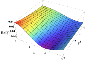
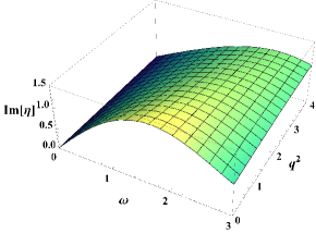
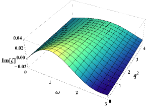
Figure 1: The viscosities $\eta(\omega,q^{2})$ and $\zeta(\omega,q^{2})$ as functions of $\omega$ and $q^{2}$.

The real parts of $\eta$ and $\zeta$ decrease with momenta until reaching minima around points $\left\{\omega\approx 3.0,q^{2}=0\right\}$ and $\left\{\omega\approx 1.9,q^{2}=0\right\}$, respectively. A sign of damped oscillations is observed in the results, while eventually, the real parts vanish at very large $\omega$ and/or $q^{2}$. The imaginary parts of the viscosities first increase from zero up to some maxima around $\left\{\omega\approx 1.7,q^{2}=0\right\}$ for $\eta$ and $\left\{\omega\approx 1.0,q^{2}=0\right\}$ for $\zeta$. With further increase of the momenta, the imaginary parts decrease reaching zero at large momenta.

Vanishing of transport coefficients at very large momenta is well anticipated: there should be no response at very short times or distances. This point is critical for the generalized relativistic hydrodynamics to be causal. To further confirm our observation, we focus on large momenta behavior for the viscosity functions. In Figures 2 and 3, we show our results for very large $\omega$ or $q^{2}$.

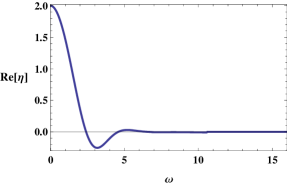
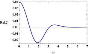
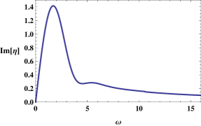
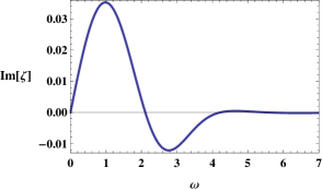
Figure 2: The generalized viscosity functions $\eta$ and $\zeta$ vs $\omega$ at $q^{2}=0$.

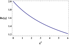
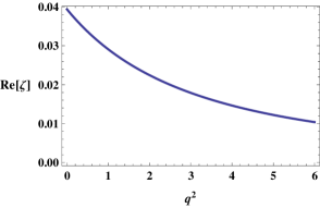
Figure 3: The generalized viscosity functions $\eta$ and $\zeta$ vs $q^{2}$ at $\omega=0$.

The imaginary parts of $\eta$ and $\zeta$ are identically zero at $\omega=0$. This is obvious from the eqs. (95), which have no imaginary terms at $\omega=0$. Vanishing of the viscosity functions at large $\omega$ (and/or $q^{2}$) is an important factor for reliably addressing early time stage in heavy ion collisions 1302.0697 ; 0704.1647 ; 1108.3972 .

The imaginary part of $\eta$ never turns negative. This is indeed a necessary condition for stability of the fluid equations, as is seen from the shear mode dispersion relation (51). In contrast, the imaginary part of $\zeta$ does change sign at intermediate values of $\omega$ and $q^{2}$ as seen in Figure 1. However, negative $\zeta$ does not mean an instability: it only contributes as a practically negligible correction to the dispersion relation of sound mode (52), but never turns any of these modes into unstable. Indeed, the absolute value of $\zeta(\omega,q^{2})$ is always highly suppressed as compared to that of $\eta(\omega,q^{2})$. Furthermore, the inequality $q^{2}\zeta(\omega,q^{2})\ll\eta(\omega,q^{2})$ is valid in all the kinematic range covered by our numerical results. Therefore, for any practical applications and hydrodynamic modelings, it is probably always safe to ignore the viscosity function $\zeta(\omega,q^{2})$.

4.2 Approximate results from the matching method

In this subsection we provide an alternative approach to solving equations (95) based on an analytic approximate scheme. This provides us with a possibility to check the numerical results of the previous subsection. The main idea is to adopt a matching method, which was introduced in 0907.3203 in order to provide analytical evidence for condensation phenomena in a holographic superconductor model 0803.3295 . The method is based on the series expansions  (96) and (97), which not only exactly solve the system (95) but also should match over the whole regime of $u\in[0,1]$.

The approximation we are to employ is a truncation of the series (96) and (97): we will keep up to eleven terms in each expansion, i.e., order $u^{10}$ and $(u-1)^{10}$, respectively. While the truncated series would not any more solve the system (95) exactly, keeping enough terms guarantees accurate solutions near the horizon and conformal boundary. We then match the truncated series solutions at an intermediate point such as $u=1/2$. Taking $\tilde{a}(\omega,q,u)$ as an example, the matching of its value and first order derivative at $u=1/2$ results in,

$$\begin{split}\sum_{n=0}^{10}A_{h}^{n}(u-1)^{n}\Bigg{|}_{u=1/2}&=\left(\sum_{n=0}^{10}A_{b}^{n}u^{n}+u^{4}\ln{u}\sum_{n=0}^{10}A_{L}^{n}u^{n}\right)\Bigg{|}_{u=1/2},\\ \left(\sum_{n=0}^{10}A_{h}^{n}(u-1)^{n}\right)^{\prime}\Bigg{|}_{u=1/2}&=\left(\sum_{n=0}^{10}A_{b}^{n}u^{n}+u^{4}\ln{u}\sum_{n=0}^{10}A_{L}^{n}u^{n}\right)^{\prime}\Bigg{|}_{u=1/2},\end{split}$$ (106)

where the boundary conditions (98) and (99) should be imposed. This method casts the system (95) into algebraic equations for these expansion coefficients. On the one hand, having kept a large number (eleven) of terms in the expansions, we achieve stable and highly accurate results. The viscosity functions obtained from the matching scheme are displayed in Figure 4.

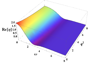
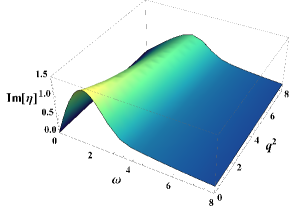
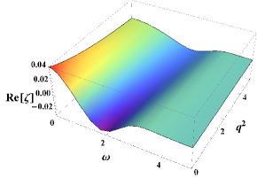
Figure 4: The viscosity functions $\eta(\omega,q^{2})$ and $\zeta(\omega,q^{2})$ vs $\omega$ and $q^{2}$ from the matching method.

On the other hand, the large number of terms kept in (106) lead to analytical but rather lengthy and not very illuminating expressions for the viscosity functions. They are of the type

$$\eta(\omega,q^{2})\approx\frac{P_{\eta}(\omega,q^{2})}{Q_{\eta}(\omega,q^{2})},~{}~{}~{}~{}~{}~{}~{}~{}~{}\zeta(\omega,q^{2})\approx\frac{P_{\zeta}(\omega,q^{2})}{Q_{\zeta}(\omega,q^{2})}.$$ (107)

where $P$s and $Q$s are finite order polynomials in $\omega$ and $q^{2}$. Below, we only quote a few terms in hydrodynamic expansion of these polynomials,

$$\begin{split}P_{\eta}(\omega,q^{2})=&2.00-1.82i\omega-1.01\omega^{2}+0.249q^{2}-0.208i\omega q^{2}+0.401i\omega^{3}-0.103\omega^{2}q^{2}\\ &+0.124\omega^{4}+0.0119q^{4}+\cdots,\\ Q_{\eta}(\omega,q^{2})=&1.00-1.56i\omega-1.24\omega^{2}+0.250q^{2}-0.296i\omega q^{2}+0.656i\omega^{3}-0.189\omega^{2}q^{2}\\ &+0.255\omega^{4}+0.0178q^{4}++0.0822i\omega^{3}q^{2}-0.0780i\omega^{5}+\cdots,\\ P_{\zeta}(\omega,q^{2})=&0.0396-0.0666i\omega-0.0611\omega^{2}+0.00772q^{2}+\cdots,\\ Q_{\zeta}(\omega,q^{2})=&1.00-3.13i\omega-4.93\omega^{2}+0.526q^{2}-1.44i\omega q^{2}+5.20i\omega^{3}-2.01\omega^{2}q^{2}\\ &+4.11\omega^{4}+0.107q^{4}+1.89i\omega^{3}q^{2}-2.59i\omega^{5}+\cdots.\end{split}$$ (108)

The structure (107) implies that the viscosities have a number of poles (zeros of $Q$s) and this is quite consistent with the arguments made in 0905.4069 that exact $\eta(\omega,q^{2})$ in fact has infinitely many poles.

In the hydrodynamic limit, our approximate results for the viscosities are

$$\begin{split}\eta_{\text{m}}(\omega,q^{2})&=2.00+1.31i\omega-0.567\omega^{2}-0.252q^{2}-0.337i\omega q^{2}\\ &-0.169i\omega^{3}+0.243\omega^{2}q^{2}+0.0306\omega^{4}+0.0395q^{4}+\cdots,\\ \zeta_{\text{m}}(\omega,q^{2})&=0.0396+0.0573i\omega-0.0449\omega^{2}-0.0131q^{2}+\cdots,\end{split}$$ (109)

They are in perfect agreement with the analytical results of section 3 as quoted in (9), with up to $1\%$ error. We notice that the expansion (109) provides an extension of our analytical third order result to much higher order.

The obtained approximate results make it possible to explore the asymptotic behavior of the viscosity functions in the limit of very large momenta,

$$\eta(\omega,q^{2})\sim\frac{i}{\omega},~{}~{}~{}~{}\zeta(\omega,q^{2})\sim-\frac{i}{\omega^{3}},~{}~{}~{}\text{as}~{}~{}~{}\omega\to\infty~{}\text{and}~{}q^{2}\to\infty.$$ (110)

This asymptotic behavior of (110) provides another confirmation for vanishing of $\eta$ and $\zeta$ in the large momenta regime.

5 Summary and discussion

In this paper we have provided all the details and expanded presentation of the results advertised in our short publication 1406.7222 . As a further development of the ideas put forward in 0704.1647 , we have consistently determined the energy-momentum stress tensor of a weakly perturbed conformal fluid, whose underlying microscopic description is a strongly coupled $\mathcal{N}=4$ super-Yang-Mills theory at finite temperature. The results were derived by linearizing the fluid/gravity correspondence. We have included all order derivative terms in the boundary stress tensor, limiting the study to small amplitude perturbations only. We have found that all order dissipative terms in the fluid stress tensor are fully accounted for by two (generalized) momenta-dependent viscosity functions $\eta(\omega,q^{2})$ and $\zeta(\omega,q^{2})$. $\eta(\omega,q^{2})$ is a transport coefficient in front of the shear tensor $\sigma_{ij}$ while $\zeta(\omega,q^{2})$ is a coefficient of a new tensor $\pi_{ij}$, which is given in terms of third order derivative of the fluid velocity.

As one of our main results, we have derived a closed-form linear holographic RG flow-type equations (42) for the viscosity functions. Intriguingly, an analogous holographic RG flow equation for electrical conductivity obtained in 0809.3808 is a nonlinear one. The constraint components of the bulk Einstein equations (11) have been shown to generalize the Navier-Stokes equations, consistently with the conservation laws of the fluid stress tensor. We have analytically computed the viscosity functions, up to third order in the hydrodynamic gradient expansion, and the dispersion relations for the shear and sound waves. These third order corrections are needed in order to correctly reproduce the dispersion relation for the shear wave up to order $\mathcal{O}(q^{4})$, as emphasized in 0712.2451 ; 0712.2456 .

To include all order dissipative effects in the fluid stress tensor, we have solved numerically the RG flow-type equations (42). The numerical results for the viscosity functions are displayed in Figure 1. Based on our numerical calculations, we have been able to significantly extend knowledge about the viscosity functions in the hydrodynamic limit, providing in (109) an expansion up to fifth order. Consistently with physical intuition, the viscosities vanish at very large momenta as seen in Figures 2 and 3. We have verified our results by solving the equations (42) using an alternative method.

Importantly, the hydrodynamic theory constructed in this work is causal and should be free of any instabilities if implemented as a dynamical model for plasma evolution. The viscosity function encodes an infinite set of quasi-normal modes hep-th/0506184 including corresponding residues.

Obviously, this is not QCD, but we hope that some generic features about momenta-dependent transport coefficients and high gradient structures have been captured by our results. They can help in building new models of causal relativistic hydrodynamics, beyond Navier-Stokes or Israel-Stewart.

The stress tensor computed in this work resums all order gradients linearized in the amplitude of fluid velocity and is not readily applicable to phenomena where nonlinearities are important, such as Bjorken flow. Nevertheless, the results reported here might be useful both in estimating phenomenological roles and sizes of higher gradient effects as suggested in 0704.1647 ; 0905.4069 and in direct studies of experimentally observed phenomena where linear dissipative terms play an important role. Sonic booms created by jets or heavy quarks, fluctuations in the flows and correlations are examples of applications which we have in mind.

A question of convergence of the gradient expansion has been raised in 1302.0697 , and it has been argued there that radius of convergence is in fact zero presumably due to a factorial growth in the number of terms at high orders. We have not observed any convergence issues, thus indirectly confirming the conclusions of 1302.0697 about a nonlinear origin of the convergence problem.

Throughout the paper, we have been referring to equations (42) as holographic RG flow-type equations for the viscosity functions. Indeed, the radial coordinate $r$ is frequently associated with a scale of RG flow of the boundary CFT. While we do have an evolution in $r$, we identify physical quantities (viscosities) only at the infinite boundary. In the spirit of holographic Wilsonian RG 1006.1902 ; 1009.3094 ; 1010.1264 ; 1010.4036 ; 1102.4477 ; 1107.2134 , it would be proper to introduce a finite cutoff along radial direction and define associated physical quantities, such as $\eta(r,\omega,q^{2})$ and $\zeta(r,\omega,q^{2})$, at the cutoff surface. That would result in an RG evolution of these momenta-dependent coefficients, thus extending previous results on RG flows of the shear viscosity coefficient $\eta_{0}$. So far, the universality of the ratio (6) was clarified as a consequence of no RG flow from the horizon to the boundary of the Navier-Stokes hydrodynamics 0809.3808 .

As further development of this project, we plan to extend our present study to conformal fluids in a weakly curved background manifold, with all order derivative terms resummed. Metric perturbations at the boundary may be taken into account following 0806.0006 ; 0809.4272 . Additional transport coefficient functions associated with the boundary curvature are expected to emerge 0905.4069 .

- (1) Y. Bu and M. Lublinsky, “All Order Linearized Hydrodynamics from Fluid/Gravity Correspondence,” Phys.Rev. D90 (2014) 086003, arXiv:1406.7222 [hep-th].
- (2) M. Gyulassy and L. McLerran, “New forms of QCD matter discovered at RHIC,” Nucl.Phys. A750 (2005) 30–63, arXiv:nucl-th/0405013 [nucl-th].
- (3) E. V. Shuryak, “What RHIC experiments and theory tell us about properties of quark-gluon plasma?,” Nucl.Phys. A750 (2005) 64–83, arXiv:hep-ph/0405066 [hep-ph].
- (4) Y. Aoki, G. Endrodi, Z. Fodor, S. Katz, and K. Szabo, “The Order of the quantum chromodynamics transition predicted by the standard model of particle physics,” Nature 443 (2006) 675–678, arXiv:hep-lat/0611014 [hep-lat].
- (5) S. Borsanyi, G. Endrodi, Z. Fodor, A. Jakovac, S. D. Katz, et al., “The QCD equation of state with dynamical quarks,” JHEP 1011 (2010) 077, arXiv:1007.2580 [hep-lat].
- (6) S. Borsanyi, Z. Fodor, C. Hoelbling, S. D. Katz, S. Krieg, et al., “Full result for the QCD equation of state with 2+1 flavors,” Phys.Lett. B730 (2014) 99–104, arXiv:1309.5258 [hep-lat].
- (7) L. D. Landau and E. M. Lifshitz, Fluid Mechanics: Course of Theoretical Physics, Vol. 6. Butterworth-Heinemann, 1965.
- (8) L. Rezzolla and O. Zanotti, Relativistic Hydrodynamics. Oxford University Press, 2013.
- (9) W. Hiscock and L. Lindblom, “Stability and causality in dissipative relativistic fluids,” Annals Phys. 151 (1983) 466–496.
- (10) W. A. Hiscock and L. Lindblom, “Generic instabilities in first-order dissipative relativistic fluid theories,” Phys.Rev. D31 (1985) 725–733.
- (11) W. A. Hiscock and L. Lindblom, “Linear plane waves in dissipative relativistic fluids,” Phys.Rev. D35 (1987) 3723–3732.
- (12) W. Hiscock and L. Lindblom, “Nonlinear pathologies in relativistic heat-conducting fluid theories,” Phys.Lett. A131 (1988) 509–513.
- (13) W. Israel, “Nonstationary irreversible thermodynamics: A Causal relativistic theory,” Annals Phys. 100 (1976) 310–331.
- (14) W. Israel and J. Stewart, “Transient relativistic thermodynamics and kinetic theory,” Annals Phys. 118 (1979) 341–372.
- (15) S. Pu, T. Koide, and D. H. Rischke, “Does stability of relativistic dissipative fluid dynamics imply causality?,” Phys.Rev. D81 (2010) 114039, arXiv:0907.3906 [hep-ph].
- (16) G. Denicol, T. Kodama, T. Koide, and P. Mota, “Stability and Causality in relativistic dissipative hydrodynamics,” J.Phys. G35 (2008) 115102, arXiv:0807.3120 [hep-ph].
- (17) G. S. Denicol, J. Noronha, H. Niemi, and D. H. Rischke, “Origin of the Relaxation Time in Dissipative Fluid Dynamics,” Phys.Rev. D83 (2011) 074019, arXiv:1102.4780 [hep-th].
- (18) J. M. Maldacena, “The Large N limit of superconformal field theories and supergravity,” Adv.Theor.Math.Phys. 2 (1998) 231–252, arXiv:hep-th/9711200 [hep-th].
- (19) S. Gubser, I. R. Klebanov, and A. M. Polyakov, “Gauge theory correlators from noncritical string theory,” Phys.Lett. B428 (1998) 105–114, arXiv:hep-th/9802109 [hep-th].
- (20) E. Witten, “Anti-de Sitter space and holography,” Adv.Theor.Math.Phys. 2 (1998) 253–291, arXiv:hep-th/9802150 [hep-th].
- (21) O. Aharony, S. S. Gubser, J. M. Maldacena, H. Ooguri, and Y. Oz, “Large N field theories, string theory and gravity,” Phys.Rept. 323 (2000) 183–386, arXiv:hep-th/9905111 [hep-th].
- (22) G. Policastro, D. T. Son, and A. O. Starinets, “The Shear viscosity of strongly coupled N=4 supersymmetric Yang-Mills plasma,” Phys.Rev.Lett. 87 (2001) 081601, arXiv:hep-th/0104066 [hep-th].
- (23) G. Policastro, D. T. Son, and A. O. Starinets, “From AdS / CFT correspondence to hydrodynamics,” JHEP 0209 (2002) 043, arXiv:hep-th/0205052 [hep-th].
- (24) P. Kovtun, D. T. Son, and A. O. Starinets, “Viscosity in strongly interacting quantum field theories from black hole physics,” Phys.Rev.Lett. 94 (2005) 111601, arXiv:hep-th/0405231 [hep-th].
- (25) R. A. Janik and R. B. Peschanski, “Asymptotic perfect fluid dynamics as a consequence of Ads/CFT,” Phys.Rev. D73 (2006) 045013, arXiv:hep-th/0512162 [hep-th].
- (26) A. Buchel and J. T. Liu, “Universality of the shear viscosity in supergravity,” Phys.Rev.Lett. 93 (2004) 090602, arXiv:hep-th/0311175 [hep-th].
- (27) A. Buchel, R. C. Myers, M. F. Paulos, and A. Sinha, “Universal holographic hydrodynamics at finite coupling,” Phys.Lett. B669 (2008) 364–370, arXiv:0808.1837 [hep-th].
- (28) N. Iqbal and H. Liu, “Universality of the hydrodynamic limit in AdS/CFT and the membrane paradigm,” Phys.Rev. D79 (2009) 025023, arXiv:0809.3808 [hep-th].
- (29) Y. Kats and P. Petrov, “Effect of curvature squared corrections in AdS on the viscosity of the dual gauge theory,” JHEP 0901 (2009) 044, arXiv:0712.0743 [hep-th].
- (30) M. Brigante, H. Liu, R. C. Myers, S. Shenker, and S. Yaida, “Viscosity Bound Violation in Higher Derivative Gravity,” Phys.Rev. D77 (2008) 126006, arXiv:0712.0805 [hep-th].
- (31) R. C. Myers, M. F. Paulos, and A. Sinha, “Quantum corrections to eta/s,” Phys.Rev. D79 (2009) 041901, arXiv:0806.2156 [hep-th].
- (32) A. Buchel, R. C. Myers, and A. Sinha, “Beyond eta/s = 1/4 pi,” JHEP 0903 (2009) 084, arXiv:0812.2521 [hep-th].
- (33) R.-G. Cai, Z.-Y. Nie, and Y.-W. Sun, “Shear Viscosity from Effective Couplings of Gravitons,” Phys.Rev. D78 (2008) 126007, arXiv:0811.1665 [hep-th].
- (34) R.-G. Cai, Z.-Y. Nie, N. Ohta, and Y.-W. Sun, “Shear Viscosity from Gauss-Bonnet Gravity with a Dilaton Coupling,” Phys.Rev. D79 (2009) 066004, arXiv:0901.1421 [hep-th].
- (35) X.-H. Ge and S.-J. Sin, “Shear viscosity, instability and the upper bound of the Gauss-Bonnet coupling constant,” JHEP 0905 (2009) 051, arXiv:0903.2527 [hep-th].
- (36) R. C. Myers, M. F. Paulos, and A. Sinha, “Holographic Hydrodynamics with a Chemical Potential,” JHEP 0906 (2009) 006, arXiv:0903.2834 [hep-th].
- (37) S. Cremonini, K. Hanaki, J. T. Liu, and P. Szepietowski, “Higher derivative effects on eta/s at finite chemical potential,” Phys.Rev. D80 (2009) 025002, arXiv:0903.3244 [hep-th].
- (38) R. Brustein and A. Medved, “Proof of a universal lower bound on the shear viscosity to entropy density ratio,” Phys.Lett. B691 (2010) 87–90, arXiv:0908.1473 [hep-th].
- (39) J. Erdmenger, P. Kerner, and H. Zeller, “Non-universal shear viscosity from Einstein gravity,” Phys.Lett. B699 (2011) 301–304, arXiv:1011.5912 [hep-th].
- (40) P. Basu and J.-H. Oh, “Analytic Approaches to Anisotropic Holographic Superfluids,” JHEP 1207 (2012) 106, arXiv:1109.4592 [hep-th].
- (41) A. Rebhan and D. Steineder, “Violation of the Holographic Viscosity Bound in a Strongly Coupled Anisotropic Plasma,” Phys.Rev.Lett. 108 (2012) 021601, arXiv:1110.6825 [hep-th].
- (42) R. Critelli, S. Finazzo, M. Zaniboni, and J. Noronha, “Anisotropic shear viscosity of a strongly coupled non-Abelian plasma from magnetic branes,” Phys.Rev. D90 (2014) 066006, arXiv:1406.6019 [hep-th].
- (43) D. T. Son and A. O. Starinets, “Viscosity, Black Holes, and Quantum Field Theory,” Ann.Rev.Nucl.Part.Sci. 57 (2007) 95–118, arXiv:0704.0240 [hep-th].
- (44) S. Bhattacharyya, V. E. Hubeny, S. Minwalla, and M. Rangamani, “Nonlinear Fluid Dynamics from Gravity,” JHEP 0802 (2008) 045, arXiv:0712.2456 [hep-th].
- (45) R. Baier, P. Romatschke, D. T. Son, A. O. Starinets, and M. A. Stephanov, “Relativistic viscous hydrodynamics, conformal invariance, and holography,” JHEP 0804 (2008) 100, arXiv:0712.2451 [hep-th].
- (46) M. Haack and A. Yarom, “Nonlinear viscous hydrodynamics in various dimensions using AdS/CFT,” JHEP 0810 (2008) 063, arXiv:0806.4602 [hep-th].
- (47) S. Bhattacharyya, R. Loganayagam, I. Mandal, S. Minwalla, and A. Sharma, “Conformal Nonlinear Fluid Dynamics from Gravity in Arbitrary Dimensions,” JHEP 0812 (2008) 116, arXiv:0809.4272 [hep-th].
- (48) S. Bhattacharyya, R. Loganayagam, S. Minwalla, S. Nampuri, S. P. Trivedi, et al., “Forced Fluid Dynamics from Gravity,” JHEP 0902 (2009) 018, arXiv:0806.0006 [hep-th].
- (49) M. Rangamani, “Gravity and Hydrodynamics: Lectures on the fluid-gravity correspondence,” Class.Quant.Grav. 26 (2009) 224003, arXiv:0905.4352 [hep-th].
- (50) V. E. Hubeny, S. Minwalla, and M. Rangamani, “The fluid/gravity correspondence,” arXiv:1107.5780 [hep-th].
- (51) M. Lublinsky and E. Shuryak, “How much entropy is produced in strongly coupled Quark-Gluon Plasma (sQGP) by dissipative effects?,” Phys.Rev. C76 (2007) 021901, arXiv:0704.1647 [hep-ph].
- (52) M. Lublinsky and E. Shuryak, “Improved Hydrodynamics from the AdS/CFT,” Phys.Rev. D80 (2009) 065026, arXiv:0905.4069 [hep-ph].
- (53) M. P. Heller, R. A. Janik, and P. Witaszczyk, “The characteristics of thermalization of boost-invariant plasma from holography,” Phys.Rev.Lett. 108 (2012) 201602, arXiv:1103.3452 [hep-th].
- (54) M. P. Heller, R. A. Janik, and P. Witaszczyk, “A numerical relativity approach to the initial value problem in asymptotically Anti-de Sitter spacetime for plasma thermalization - an ADM formulation,” Phys.Rev. D85 (2012) 126002, arXiv:1203.0755 [hep-th].
- (55) M. P. Heller, R. A. Janik, and P. Witaszczyk, “Hydrodynamic Gradient Expansion in Gauge Theory Plasmas,” Phys.Rev.Lett. 110 (2013) 211602, arXiv:1302.0697 [hep-th].
- (56) D. T. Son and A. O. Starinets, “Minkowski space correlators in AdS / CFT correspondence: Recipe and applications,” JHEP 0209 (2002) 042, arXiv:hep-th/0205051 [hep-th].
- (57) P. Kovtun and A. Starinets, “Thermal spectral functions of strongly coupled N=4 supersymmetric Yang-Mills theory,” Phys.Rev.Lett. 96 (2006) 131601, arXiv:hep-th/0602059 [hep-th].
- (58) M. P. Heller and R. A. Janik, “Viscous hydrodynamics relaxation time from AdS/CFT,” Phys.Rev. D76 (2007) 025027, arXiv:hep-th/0703243 [HEP-TH].
- (59) M. Natsuume and T. Okamura, “Causal hydrodynamics of gauge theory plasmas from AdS/CFT duality,” Phys.Rev. D77 (2008) 066014, arXiv:0712.2916 [hep-th].
- (60) M. Haack and A. Yarom, “Universality of second order transport coefficients from the gauge-string duality,” Nucl.Phys. B813 (2009) 140–155, arXiv:0811.1794 [hep-th].
- (61) V. Balasubramanian and P. Kraus, “A Stress tensor for Anti-de Sitter gravity,” Commun.Math.Phys. 208 (1999) 413–428, arXiv:hep-th/9902121 [hep-th].
- (62) M. Henningson and K. Skenderis, “The Holographic Weyl anomaly,” JHEP 9807 (1998) 023, arXiv:hep-th/9806087 [hep-th].
- (63) P. K. Kovtun and A. O. Starinets, “Quasinormal modes and holography,” Phys.Rev. D72 (2005) 086009, arXiv:hep-th/0506184 [hep-th].
- (64) W. H. Press, S. A. Teukolsky, W. T. Vetterling, and B. P. Flannery, Numerical Recipes: The Art of Scientific Computing. Cambridge University Press, 2007.
- (65) M. Lublinsky and E. Shuryak, “Universal hydrodynamics and charged hadron multiplicity at the LHC,” Phys.Rev. C84 (2011) 061901, arXiv:1108.3972 [hep-ph].
- (66) R. Gregory, S. Kanno, and J. Soda, “Holographic Superconductors with Higher Curvature Corrections,” JHEP 0910 (2009) 010, arXiv:0907.3203 [hep-th].
- (67) S. A. Hartnoll, C. P. Herzog, and G. T. Horowitz, “Building a Holographic Superconductor,” Phys.Rev.Lett. 101 (2008) 031601, arXiv:0803.3295 [hep-th].
- (68) I. Bredberg, C. Keeler, V. Lysov, and A. Strominger, “Wilsonian Approach to Fluid/Gravity Duality,” JHEP 1103 (2011) 141, arXiv:1006.1902 [hep-th].
- (69) D. Nickel and D. T. Son, “Deconstructing holographic liquids,” New J.Phys. 13 (2011) 075010, arXiv:1009.3094 [hep-th].
- (70) I. Heemskerk and J. Polchinski, “Holographic and Wilsonian Renormalization Groups,” JHEP 1106 (2011) 031, arXiv:1010.1264 [hep-th].
- (71) T. Faulkner, H. Liu, and M. Rangamani, “Integrating out geometry: Holographic Wilsonian RG and the membrane paradigm,” JHEP 1108 (2011) 051, arXiv:1010.4036 [hep-th].
- (72) S.-J. Sin and Y. Zhou, “Holographic Wilsonian RG Flow and Sliding Membrane Paradigm,” JHEP 1105 (2011) 030, arXiv:1102.4477 [hep-th].
- (73) C. Eling and Y. Oz, “Holographic Screens and Transport Coefficients in the Fluid/Gravity Correspondence,” Phys.Rev.Lett. 107 (2011) 201602, arXiv:1107.2134 [hep-th].