Strongly Intensive Measures for Particle Number Fluctuations:
Effects of Hadronic Resonances

Abstract

Strongly intensive measures $\Delta$ and $\Sigma$ are used to study event-by-event fluctuations of hadron multiplicities in nucleus-nucleus collisions. The effects of resonance decays are investigated within statistical model and relativistic transport model. Two specific examples are considered: resonance decays to two positively charged particles (e.g., $\Delta^{++}\rightarrow p+\pi^{+}$) and to $\pi^{+}\pi^{-}$-pairs. (e.g., $\rho^{0}\rightarrow\pi^{-}+\pi^{+}$). It is shown that resonance abundances at the chemical freeze-out can be estimated by measuring the fluctuations of the number of stable hadrons. These model results are compared to the full hadron-resonance gas analysis within both the grand canonical and canonical ensemble. The ultra-relativistic quantum molecular dynamics (UrQMD) model of nucleus-nucleus collisions is used to illustrate the role of global charge conservation, centrality selection, and limited experimental acceptance.

I Introduction

The main physics motivation for the experimental investigations of relativistic nucleus-nucleus (A+A) collisions started at mid 1980s was to create and study the strongly interacting matter in its different phases: the hadron-resonance gas and the quark-gluon plasma. Today these studies are still in progress at the Super Proton Synchrotron (SPS) of the European Organization for Nuclear Research (CERN) and at the Relativistic Heavy Ion Collider (RHIC) of Brookhaven National Laboratory (BNL); they are pursued also at much higher collision energies at the Large Hadron Collider (LHC) at CERN. A possibility to observe signatures of the critical point of the QCD matter inspired the energy and system size scan program of the NA61/SHINE Collaboration at the CERN SPS Ga:2009 and the low energy scan program of the STAR and PHENIX Collaborations at the BNL RHIC RHIC-SCAN .

Experimental and theoretical investigations of the event-by-event (e-by-e) fluctuations in A+A collisions are relevant for current and future studies of the onset of deconfinement and the search for the critical point (see, e.g., recent review GGS and references therein). These investigations, however, have been confronted with a serious problem. The e-by-e fluctuations of the number of nucleon participants affect strongly the fluctuations of any physical observables KGBG:2010 . In the language of statistical mechanics, this is equivalent to the system volume fluctuations. Note that in high energy A+A collisions the system volume fluctuations can be hardly avoided. Besides, the average volume of the created matter and its variations from collision to collision are usually difficult or even impossible to be measured. Therefore, a choice of adequate statistical tools is crucially important for a study of the e-by-e fluctuations in A+A collisions.

In the present paper we use the strongly intensive measures of fluctuations GG:2011 . In a framework of several popular models of A+A collisions, these quantities are independent of both the average volume of a system and the volume fluctuations. For example, this is valid within the grand canonical formulation of statistical mechanics. An analysis of the yields of different hadronic species in A+A collisions demonstrates that a statistical model of the hadron-resonance gas gives an impressive agreement with a large amount of data in terms of a few adjusting parameters. Using statistical approach the effects of resonance decays for the particle number fluctuations and correlations are considered in terms of the strongly intensive measures. We discuss two examples for which the e-by-e fluctuations of hadron multiplicities are rather sensitive to the abundances of resonances at the chemical freeze-out. As a result, these resonance abundances, which are difficult to be measured by other methods, can be estimated by measuring the fluctuations and correlations of the numbers of stable hadrons. Note that an idea to use the e-by-e fluctuations of particle number ratios to estimate the number of hadronic resonances was suggested for the first time by Jeon and Koch in Ref. JK .

The paper is organized as follows. In Sec. II the notions of strongly intensive measures and volume fluctuations in thermal systems are considered. Sec. III presents two simple examples of analytical calculations: first, resonance decays into two positive hadrons and, second, into $\pi^{+}\pi^{-}$-pairs. In Sec. IV these two model examples are tested within the full hadron-resonance gas model. In Sec. V the ultra-relativistic quantum molecular dynamics (UrQMD) model is used in Pb+Pb and proton-proton ($p+p$) collisions at the SPS energies to illustrate the role of global charge conservation, centrality selection, and limited experimental acceptance. A summary in Sec. VI closes the article.

II Strongly Intensive Quantities

The strongly intensive quantities $\Delta$ and $\Sigma$ have been introduced in Ref. GG:2011 . Within the grand canonical ensemble (GCE) formulation of statistical mechanics they are independent of the average volume and volume fluctuations. Similar properties take place in the model of independent sources: the strongly intensive measures of fluctuations are independent of the average number of sources and of fluctuations of the number of sources.

Note that the first strongly intensive measure of fluctuations, the so-called $\Phi$ measure, was introduced a long time ago in Ref. GM:1992 . There were many attempts to use the $\Phi$ measure in the data analysis Phi_data ; d1 ; d2 ; d3 ; d4 ; d5 ; d6 and in theoretical models Phi_models ; m2 ; m3 ; m4 ; m5 ; m6 ; m7 ; m8a ; m8 ; m9 ; m10 ; m11 ; MRW:2004 ; m12 ; m13 ; m14 . The measures $\Delta$ and $\Sigma$ have several advantages: they are dimensionless and give a common scale required for a quantitative comparison of the e-by-e fluctuations (see more details in Ref. GGP:2013 ).

The strongly intensive measures $\Delta$ and $\Sigma$ are defined using two extensive quantities, i.e. the quantities proportional to the system volume. A popular example of such a pair of extensive variables is: the transverse momentum $P_{T}=p_{T}^{(1)}+\dots p_{T}^{(N)}$, where $p^{(i)}_{T}$ is the absolute value of the $i^{{\rm th}}$ particle transverse momentum, and the number of particles $N$. The measures $\Delta[P_{T},N]$ and $\Sigma[P_{T},N]$ were studied recently within the UrQMD simulations in Ref. KG:APP2012 ; GGP:2013 and within the GCE formulation for the ideal Bose and Fermi gases in Ref. GR:2013 . The basic properties of the $\Delta[P_{T},N]$ and $\Sigma[P_{T},N]$ measures were also tested using the Monte Carlo simulations and analytical models in Ref. GG:2014 .

The measures $\Delta[K,\pi]$ and $\Sigma[K,\pi]$, in the case of multiplicities of charged kaons, $K=K^{+}+K^{-}$, and pions, $\pi=\pi^{+}+\pi^{-}$, were considered within the hadron-string dynamics transport model in Ref. HSD . Note that the NA49 and NA61/SHINE Collaborations have already started to use the strongly intensive measures $\Delta$ and $\Sigma$ for the studies of e-by-e fluctuations in $p+p$ and A+A collisions (see Ref. GGS and references therein).

In the present paper the strongly intensive measures for particle number fluctuations are studied GG:2011 :

$$\Delta[N_{1},N_{2}]\leavevmode\nobreak\ =\leavevmode\nobreak\ \frac{1}{C_{\Delta}}\Big{[}\langle N_{2}\rangle\,\omega[N_{1}]\leavevmode\nobreak\ -\leavevmode\nobreak\ \langle N_{1}\rangle\,\omega[N_{2}]\Big{]}\leavevmode\nobreak\ ,$$ (1)

$$\Sigma[N_{1},N_{2}]\leavevmode\nobreak\ =\leavevmode\nobreak\ \frac{1}{C_{\Sigma}}\Big{[}\langle N_{1}\rangle\,\omega[N_{2}]\leavevmode\nobreak\ +\leavevmode\nobreak\ \langle N_{2}\rangle\,\omega[N_{1}]\leavevmode\nobreak\ -\leavevmode\nobreak\ 2\Big{(}\langle N_{1}\,N_{2}\rangle\leavevmode\nobreak\ -\leavevmode\nobreak\ \langle N_{1}\rangle\langle N_{2}\rangle\Big{)}\Big{]}\leavevmode\nobreak\ ,$$ (2)

where $N_{1}$ and $N_{2}$ are the multiplicities for hadrons of types 1 and 2,

$$\omega[N_{1}]\leavevmode\nobreak\ =\leavevmode\nobreak\ \frac{\langle N_{1}^{2}\rangle\leavevmode\nobreak\ -\leavevmode\nobreak\ \langle N_{1}\rangle^{2}}{\langle N_{1}\rangle}\leavevmode\nobreak\ ,\leavevmode\nobreak\ \leavevmode\nobreak\ \leavevmode\nobreak\ \leavevmode\nobreak\ \omega[N_{2}]\leavevmode\nobreak\ =\leavevmode\nobreak\ \frac{\langle N_{2}^{2}\rangle\leavevmode\nobreak\ -\leavevmode\nobreak\ \langle N_{2}\rangle^{2}}{\langle N_{2}\rangle}\leavevmode\nobreak\$$ (3)

are the scaled variances of $N_{1}$ and $N_{2}$ distributions, and $C_{\Delta}$ and $C_{\Sigma}$ are the normalization factors. A notation $\langle\dots\rangle$ represents the e-by-e averaging.

In a classical thermal system of non-interacting particles within the GCE formulation, the partition function $Z$ for a mixture of particles of types 1 and 2 is equal to

$$Z\leavevmode\nobreak\ =\leavevmode\nobreak\ \sum_{N_{1}=0}^{\infty}\sum_{N_{2}=0}^{\infty}\frac{z_{1}^{N_{1}}}{N_{1}!}\leavevmode\nobreak\ \frac{z_{2}^{N_{2}}}{N_{2}!}\leavevmode\nobreak\ ,$$ (4)

where $z_{i}$ ($i=1,2$) is the so called one-particle partition function,

$$z_{i}\leavevmode\nobreak\ =\leavevmode\nobreak\ V\,\exp\left(\frac{\mu_{i}}{T}\right)\,\frac{d_{i}m_{i}^{2}T}{2\pi^{2}}\,K_{2}\left(\frac{m_{i}}{T}\right)\leavevmode\nobreak\ .$$ (5)

In Eq. (5), $d_{i}$, $m_{i}$, and $\mu_{i}$ are, respectively, the degeneracy factor, mass, and chemical potential for particles of the $i$th type, whereas $V$ and $T$ are the system volume and temperature, respectively. According to Eq. (4) a joint probability distribution ${\cal P}(N_{1},N_{2})$ for variables $N_{1}$ and $N_{2}$ is just a simple product of two Poissonian distributions

$${\cal P}(N_{1},N_{2})\leavevmode\nobreak\ =\leavevmode\nobreak\ \frac{1}{Z}\,\frac{z_{1}^{N_{1}}}{N_{1}!}\,\frac{z_{2}^{N_{2}}}{N_{2}!}\leavevmode\nobreak\ =\leavevmode\nobreak\ P(N_{1})\,P(N_{2})\leavevmode\nobreak\ ,$$ (6)

with

$$P(N_{i})\leavevmode\nobreak\ =\leavevmode\nobreak\ \frac{\langle N_{i}\rangle^{N_{i}}}{N_{i}!}\,\exp\left(-\,\langle N_{i}\rangle\right)\leavevmode\nobreak\ .$$ (7)

Taking e-by-e averaging with a probability distribution ${\cal P}(N_{1},N_{2})$ (6), one finds

$$\omega[N_{1}]\leavevmode\nobreak\ =\leavevmode\nobreak\ \omega[N_{2}]\leavevmode\nobreak\ =\leavevmode\nobreak\ 1\leavevmode\nobreak\ ,$$ (8)

$$\langle N_{1}N_{2}\rangle\leavevmode\nobreak\ -\leavevmode\nobreak\ \langle N_{1}\rangle\langle N_{2}\rangle\leavevmode\nobreak\ =\leavevmode\nobreak\ 0\leavevmode\nobreak\ .$$ (9)

According to Eq. (9) there are no correlations between $N_{1}$ and $N_{2}$ numbers in the ideal Boltzmann gas within the GCE.

In Ref. GGP:2013 the special normalization has been proposed for the $\Delta$ and $\Sigma$ fluctuation measures. It is used in the present study, and for the case under consideration it reads:

$$C_{\Delta}\leavevmode\nobreak\ =\leavevmode\nobreak\ \langle N_{2}\rangle\leavevmode\nobreak\ -\leavevmode\nobreak\ \langle N_{1}\rangle\leavevmode\nobreak\ ,\leavevmode\nobreak\ \leavevmode\nobreak\ \leavevmode\nobreak\ \leavevmode\nobreak\ \leavevmode\nobreak\ C_{\Sigma}\leavevmode\nobreak\ =\leavevmode\nobreak\ \langle N_{1}\rangle\leavevmode\nobreak\ +\leavevmode\nobreak\ \langle N_{2}\rangle\leavevmode\nobreak\ .$$ (10)

The multi-component ideal Boltzmann gas before decays of resonances will be denoted as IB-GCE. It gives an important example of independent particle model (see Ref. GGP:2013 ). As shown above this model satisfies Eqs. (8) and (9). The special choice of normalization factors (10) leads then to

$$\Delta[N_{1},N_{2}]\leavevmode\nobreak\ =\leavevmode\nobreak\ \Sigma[N_{1},N_{2}]\leavevmode\nobreak\ =\leavevmode\nobreak\ 1\leavevmode\nobreak\ .$$ (11)

The independent particle model, together with the IB-GCE, plays an important role as the reference model. The deviations of real data from its results (11) can be used to clarify the physical properties of the system, i.e., relation (11) provides a common scale required for a quantitative comparison of the e-by-e fluctuations. Note also that with normalization factors (10), both $\Delta[N_{1},N_{2}]$ and $\Sigma[N_{1},N_{2}]$ become symmetric:

$$\Delta[N_{1},N_{2}]\leavevmode\nobreak\ =\leavevmode\nobreak\ \Delta[N_{2},N_{1}]\leavevmode\nobreak\ ,\leavevmode\nobreak\ \leavevmode\nobreak\ \leavevmode\nobreak\ \leavevmode\nobreak\ \leavevmode\nobreak\ \Sigma[N_{1},N_{2}]\leavevmode\nobreak\ =\leavevmode\nobreak\ \Sigma[N_{2},N_{1}]\leavevmode\nobreak\ .$$ (12)

Effects of quantum statistics change the results (8). Bose (Fermi) statistics leads to $\omega[N]$ larger (smaller) than unity. However, for the hadron systems created in A+A collisions the corrections due to quantum statistics are small. The largest effects are for pions at high temperature, when $\omega[N]\cong 1.1$, and negligible for other hadrons and resonances (see, e.g., Ref. HGM ). Therefore, relations (11) remain approximately valid for the quantum gases.

A presence of resonances decaying into particle species 1 and/or 2 change the results (8) and (9). Thus, relations (11) are also changed. These effects of particle number fluctuations and correlations due to decays of resonances will be a subject of our study.

Before a discussion of the effects of resonances we remind shortly the role of volume fluctuations within a thermal model. The average multiplicities are then assumed to be proportional to the system volume $V$,

$$\langle N_{1}\rangle\leavevmode\nobreak\ =\leavevmode\nobreak\ \rho_{1}\,\langle V\rangle\leavevmode\nobreak\ ,\leavevmode\nobreak\ \leavevmode\nobreak\ \leavevmode\nobreak\ \leavevmode\nobreak\ \langle N_{2}\rangle\leavevmode\nobreak\ =\leavevmode\nobreak\ \rho_{2}\,\langle V\rangle\leavevmode\nobreak\ ,$$ (13)

where $\rho_{1}$ and $\rho_{2}$ are the corresponding particle densities assumed to be independent of $V$. The scaled variances and correlations can be then presented as GG:2011 :

$$\omega[N_{1}]\leavevmode\nobreak\ =\leavevmode\nobreak\ \frac{\langle N_{1}^{2}\rangle_{V}\leavevmode\nobreak\ -\leavevmode\nobreak\ \langle N_{1}\rangle_{V}^{2}}{\langle N_{1}\rangle_{V}}\leavevmode\nobreak\ +\leavevmode\nobreak\ \rho_{1}\,\omega[V]\leavevmode\nobreak\ ,$$ (14)

$$\omega[N_{2}]\leavevmode\nobreak\ =\leavevmode\nobreak\ \frac{\langle N_{2}^{2}\rangle_{V}\leavevmode\nobreak\ -\leavevmode\nobreak\ \langle N_{2}\rangle_{V}^{2}}{\langle N_{2}\rangle_{V}}\leavevmode\nobreak\ +\leavevmode\nobreak\ \rho_{2}\,\omega[V]\leavevmode\nobreak\ ,$$ (15)

$$\langle N_{1}N_{2}\rangle\leavevmode\nobreak\ -\langle N_{1}\rangle\langle N_{2}\rangle\leavevmode\nobreak\ =\leavevmode\nobreak\ \langle N_{1}N_{2}\rangle_{V}\leavevmode\nobreak\ -\leavevmode\nobreak\ \langle N_{1}\rangle_{V}\leavevmode\nobreak\ \langle N_{2}\rangle_{V}\leavevmode\nobreak\ +\leavevmode\nobreak\ \rho_{1}\rho_{2}\,\langle V\rangle\,\omega[V]\leavevmode\nobreak\ ,$$ (16)

where $\langle\ldots\rangle_{V}$ denotes the averaging at fixed volume $V$, and $\omega[V]\equiv(\langle V^{2}\rangle-\langle V\rangle^{2})/\langle V\rangle$ describes the volume e-by-e fluctuations. The scaled variances (14,15) and correlation term (16) have additional contributions proportional to $\omega[V]$. As already mentioned, the volume fluctuations are usually rather large. Besides, it is rather difficult to control them experimentally. Thus, it is not easy to extract physical information from quantities (14-16). On the other hand, substituting Eqs. (13-16) into Eqs. (1,2) one finds that all terms proportional to $\omega[V]$ are canceled out, i.e. $\Delta[N_{1},N_{2}]$ and $\Sigma[N_{1},N_{2}]$ are independent of the average volume and volume fluctuations for the statistical systems within the GCE.

III Analytical Examples

Resonance decay is a probabilistic process. Introducing probabilities $b_{r}^{R}$ for $r$-th decay channel of $R$-th resonance and numbers $n_{i,r}^{R}$ of $i$-th final particles produced in these decay channels, one finds for the average multiplicity and scaled variance of $i$-th type of hadrons from decays of $R$-th type of resonances HGM :

$$\langle N_{i}\rangle\leavevmode\nobreak\ =\leavevmode\nobreak\ \langle n_{i}\rangle_{R}\leavevmode\nobreak\ \langle R\rangle\leavevmode\nobreak\ ,$$ (17)

$$\omega[N_{i}]\leavevmode\nobreak\ =\leavevmode\nobreak\ \frac{\sum_{r}b_{r}^{R}\,\left(n_{i,r}^{R}\right)^{2}\leavevmode\nobreak\ -\leavevmode\nobreak\ \left(\sum_{r}b_{r}^{R}\,n_{i,r}^{R}\right)^{2}}{\langle n_{i}\rangle_{R}}\leavevmode\nobreak\ +\leavevmode\nobreak\ \langle n_{i}\rangle_{R}\,\omega[R]\leavevmode\nobreak\ \equiv\leavevmode\nobreak\ \omega^{*}[N_{i}]\leavevmode\nobreak\ +\leavevmode\nobreak\ \langle n_{i}\rangle_{R}\,\omega[R]\leavevmode\nobreak\ ,$$ (18)

where $\langle R\rangle$ denotes the average number of $R$-th resonances, and $\langle n_{i}\rangle_{R}\equiv\sum_{r}b_{r}^{R}\,n_{i,r}$ means the average number of $i$-th hadrons produced from the decay of one $R$-th resonance. Note that different decay channels $r$ in Eqs. (17) and (18) are defined in a way that final state with only stable (with respect to strong and electromagnetic decays) hadrons are counted, and probabilities $b_{r}^{R}$ satisfy the normalization condition, $\sum_{r}b_{r}^{R}=1$. Resonances act as independent sources of particles: the first term $\omega^{*}[N_{i}]$ in the right hand side of Eq. (18) describes the $N_{i}$ fluctuations from a single source, and the second term appears due to the fluctuations of the number of sources.

Some examples are appropriate to illustrate Eq. (18). Let us assume a presence of two types of decay channels $1$ and $2$ with $n_{i,1}^{R}=1$ and $n_{i,2}^{R}=0$, and with the corresponding probabilities $b_{1}^{R}=p$ and $b_{2}^{R}=1-p$. It then follows from Eq. (18)

$$\omega[N_{i}]\leavevmode\nobreak\ =\leavevmode\nobreak\ 1\leavevmode\nobreak\ -\leavevmode\nobreak\ p\leavevmode\nobreak\ +\leavevmode\nobreak\ p\,\omega[R]\leavevmode\nobreak\ .$$ (19)

In the GCE formulation for the hadron-resonance gas, one finds $\omega[R]\cong 1$ as the effects of quantum statistics are negligible for resonances. From Eq. (19), one then obtains $\omega[N_{i}]\cong 1$, thus, resonance decays do not change Eq. (8). At $p\ll 1$ the main contribution to $\omega[N_{i}]$ in Eq. (19) comes from $\omega^{*}[N_{i}]=1-p\cong 1$, while at $p\cong 1$ from $p\,\omega[R]\cong 1$. However, resonance contributions to $\omega[N_{i}]$ becomes really important if there are decay channels with two particles of $i$-th type. Let us assume again two types of decay channels $1$ and $2$ with probabilities $b_{1}^{R}=p$ and $b_{2}^{R}=1-p$, for which $n_{i,1}^{R}=2$ and $n_{i,2}^{R}=0$. One then finds from Eq. (18)

$$\omega[N_{i}]\leavevmode\nobreak\ =\leavevmode\nobreak\ 2\,(1\leavevmode\nobreak\ -\leavevmode\nobreak\ p)\leavevmode\nobreak\ +\leavevmode\nobreak\ 2\,p\,\omega[R]\leavevmode\nobreak\ \cong\leavevmode\nobreak\ 2\leavevmode\nobreak\ ,$$ (20)

i.e., the scaled variance $\omega[N_{i}]$ is increased by a factor of 2. Therefore, a presence of resonances decaying to two (or more) particles of $i$-th type can enlarge $\omega[N_{i}]$ essentially.

If resonance $R$ has decay channels where particles of types 1 and 2 appears simultaneously in the final state, the correlation between numbers $N_{1}$ and $N_{2}$ appears:

$$\langle N_{1}N_{2}\rangle\leavevmode\nobreak\ -\leavevmode\nobreak\ \langle N_{1}\rangle\langle N_{2}\rangle\leavevmode\nobreak\ =\leavevmode\nobreak\ \Big{(}\langle R^{2}\rangle\leavevmode\nobreak\ -\leavevmode\nobreak\ \langle R\rangle^{2}\Big{)}\langle n_{1}\rangle_{R}\langle n_{2}\rangle_{R}\leavevmode\nobreak\$$

$$+\leavevmode\nobreak\ \langle R\rangle\Big{(}\langle n_{1}n_{2}\rangle_{R}\leavevmode\nobreak\ -\leavevmode\nobreak\ \langle n_{1}\rangle_{R}\langle n_{2}\rangle_{R}\Big{)}\leavevmode\nobreak\ \cong\leavevmode\nobreak\ \langle R\rangle\leavevmode\nobreak\ \langle n_{1}n_{2}\rangle_{R}\leavevmode\nobreak\ ,$$ (21)

where $\langle n_{1}n_{2}\rangle_{R}\equiv\sum_{r}b^{R}_{r}n_{1,r}^{R}n_{2,r}^{R}$. Thus, Eq. (9) is no more valid.

Our goal in this section will be to calculate the strongly intensive measures (1,2) for two simple analytical examples. The system of non-interacting Boltzmann particles and resonances within the GCE will be considered.

In the first example, resonances decaying into two positively charged particles are considered. The prominent example is the decay of $\Delta^{++}$-resonance, $\Delta^{++}\rightarrow p+\pi^{+}$. Note that the systems with positive net baryon number (and positive electric charge) are created in A+A or $p+p$. Thus, an effect of resonance decays into two negatively charged particles is much weaker and can be safely neglected. This is, however, not the case for RHIC and LHC energies, where the baryonic and electric charge densities are very small. Both processes – resonance decays into two positively charged and two negatively charged hadrons – become then comparable.

In the second example, the correlated pairs of charged pions coming from the decays of resonances are considered. The main source of these $\pi^{+}\pi^{-}$-pairs are meson resonances, e.g., $\rho^{0},\leavevmode\nobreak\ \omega\rightarrow\pi^{+}+\pi^{-}$.

For simplicity, in both model examples an existence of only one type of resonances decaying with probability 1 into two positively charged hadrons or into $\pi^{+}\pi^{-}$-pair is assumed. These resonances will be denoted as $R_{++}$ and $R_{\pi\pi}$, respectively. The same notations will be used for their multiplicities.

III.1 Resonance Decays to Two Positively Charged Hadrons

Resonance decays into two final particles of the same type 1 (or 2) lead to positive contributions to the corresponding scaled variance $\omega[N_{1}]$ (or $\omega[N_{2}]$). In our first model example, we consider $N_{1}=N_{-}$ and $N_{2}=N_{+}$, where $N_{-}$ and $N_{+}$ are the numbers of negatively and positively charged hadrons, respectively. We assume,

$$N_{-}\leavevmode\nobreak\ =\leavevmode\nobreak\ n_{-}\leavevmode\nobreak\ ,\leavevmode\nobreak\ \leavevmode\nobreak\ \leavevmode\nobreak\ \leavevmode\nobreak\ \leavevmode\nobreak\ \leavevmode\nobreak\ \leavevmode\nobreak\ N_{+}\leavevmode\nobreak\ =\leavevmode\nobreak\ n_{+}\leavevmode\nobreak\ +\leavevmode\nobreak\ 2R_{++}\leavevmode\nobreak\ ,$$ (22)

where $R_{++}$ is the number of resonances which decay into two positively charged hadrons, and the numbers of negatively and positively charged hadrons from other sources are denoted as $n_{-}$ and $n_{+}$, respectively. In the GCE, the numbers $n_{+}$ and $R_{++}$ are not correlated. Therefore, the particle number distribution $W(N_{+})$ is equal to:

$$W(N_{+})\leavevmode\nobreak\ =\leavevmode\nobreak\ \sum_{n_{+},R_{++}}P_{+}(n_{+})\,P_{R}(R_{++})\,\delta(N_{+}-n_{+}-2R_{++})\leavevmode\nobreak\ .$$ (23)

The first and second moments of $P_{-}(N_{-})$, $P_{+}(n_{+})$, and $P_{R}(R_{++})$ distributions are denoted as ($k=1,\,2$)

$$\langle N_{-}^{k}\rangle=\sum_{N_{-}}P_{-}(N_{-})\,N_{-}^{k}\leavevmode\nobreak\ ,\leavevmode\nobreak\ \leavevmode\nobreak\ \leavevmode\nobreak\ \leavevmode\nobreak\ \leavevmode\nobreak\ \langle n_{+}^{k}\rangle=\sum_{n_{+}}P_{+}(n_{+})\,n_{+}^{k}\leavevmode\nobreak\ ,\leavevmode\nobreak\ \leavevmode\nobreak\ \leavevmode\nobreak\ \leavevmode\nobreak\ \leavevmode\nobreak\ \langle R^{k}\rangle=\sum_{R_{++}}P_{R}(R_{++})\,R_{++}^{k}\leavevmode\nobreak\ .$$ (24)

The first and second moments of the $N_{+}$ distribution are calculated as

$$\langle N_{+}\rangle\leavevmode\nobreak\ =\leavevmode\nobreak\ \langle n_{+}\rangle\leavevmode\nobreak\ +\leavevmode\nobreak\ 2\langle R_{++}\rangle\leavevmode\nobreak\ ,\leavevmode\nobreak\ \leavevmode\nobreak\ \leavevmode\nobreak\ \leavevmode\nobreak\ \langle N_{+}^{2}\rangle\leavevmode\nobreak\ =\leavevmode\nobreak\ \langle n_{+}^{2}\rangle\leavevmode\nobreak\ +\leavevmode\nobreak\ 4\langle n_{+}\rangle\leavevmode\nobreak\ \langle R_{++}\rangle\leavevmode\nobreak\ +\leavevmode\nobreak\ 4\langle R_{++}^{2}\rangle\leavevmode\nobreak\ .$$ (25)

The scaled variance of the $N_{+}$ distribution then equals

$$\omega[N_{+}]\leavevmode\nobreak\ \equiv\leavevmode\nobreak\ \frac{\langle N_{+}^{2}\rangle\leavevmode\nobreak\ -\leavevmode\nobreak\ \langle N_{+}\rangle^{2}}{\langle N_{+}\rangle}\leavevmode\nobreak\ =\leavevmode\nobreak\ \frac{\langle n_{+}\rangle\,\omega[n_{+}]+4\langle R_{++}\rangle\,\omega[R_{++}]}{\langle N_{+}\rangle}\leavevmode\nobreak\ ,$$ (26)

and for the $\Delta$ measure (1) one finds:

$$\Delta[N_{-},N_{+}]\leavevmode\nobreak\ =\leavevmode\nobreak\ \frac{1}{\langle N_{+}\rangle-\langle N_{-}\rangle}\Big{[}\langle N_{+}\rangle\,\omega[N_{-}]\leavevmode\nobreak\ -\leavevmode\nobreak\ \langle N_{-}\rangle\leavevmode\nobreak\ \frac{\langle n_{+}\rangle\omega[n_{+}]+4\langle R_{++}\rangle\omega[R_{++}]}{\langle N_{+}\rangle}\Big{]}\leavevmode\nobreak\ .$$ (27)

Within approximations,

$$\omega[n_{+}]\leavevmode\nobreak\ \cong\omega[N_{-}]\leavevmode\nobreak\ ,\leavevmode\nobreak\ \leavevmode\nobreak\ \leavevmode\nobreak\ \leavevmode\nobreak\ \leavevmode\nobreak\ \leavevmode\nobreak\ \leavevmode\nobreak\ \omega[R_{++}]\leavevmode\nobreak\ \cong\leavevmode\nobreak\ 1\leavevmode\nobreak\ ,$$ (28)

one obtains:

$$\Delta[N_{-},N_{+}]\leavevmode\nobreak\ \cong\leavevmode\nobreak\ \omega[N_{-}]\leavevmode\nobreak\ -\leavevmode\nobreak\ \frac{2\langle N_{-}\rangle\,\langle R_{++}\rangle\,(2\leavevmode\nobreak\ -\leavevmode\nobreak\ \omega[N_{-}]\,)}{\langle N_{+}\rangle\,[\,\langle N_{+}\rangle-\langle N_{-}\rangle\,]}\leavevmode\nobreak\ .$$ (29)

From Eq. (29) it follows

$$\frac{\langle R_{++}\rangle}{\langle N_{+}\rangle}\leavevmode\nobreak\ \cong\leavevmode\nobreak\ \frac{\langle N_{+}\rangle-\langle N_{-}\rangle}{2\,\langle N_{-}\rangle\,(2-\omega[N_{-}])}\leavevmode\nobreak\ \Big{[}\,\omega[N_{-}]\leavevmode\nobreak\ -\leavevmode\nobreak\ \Delta[N_{-},N_{+}]\,\Big{]}\leavevmode\nobreak\ .$$ (30)

Note that within approximation (28), one can also calculate $\langle R_{++}\rangle$ from Eqs. (25) and (26):

$$\frac{\langle R_{++}\rangle}{\langle N_{+}\rangle}\leavevmode\nobreak\ \cong\leavevmode\nobreak\ \frac{\omega[N_{+}]\leavevmode\nobreak\ -\leavevmode\nobreak\ \omega[N_{-}]}{2\,(2-\omega[N_{-}]\,)}\leavevmode\nobreak\ ,$$ (31)

which is identical to expression (30).

For $\omega[N_{-}]\cong 1$, Eq. (30) is further simplified to

$$\frac{\langle R_{++}\rangle}{\langle N_{+}\rangle}\leavevmode\nobreak\ \cong\leavevmode\nobreak\ \frac{\langle N_{+}\rangle-\langle N_{-}\rangle}{2\,\langle N_{-}\rangle}\leavevmode\nobreak\ \Big{[}\,1\leavevmode\nobreak\ -\leavevmode\nobreak\ \Delta[N_{-},N_{+}]\,\Big{]}\leavevmode\nobreak\ .$$ (32)

III.2 Resonance Decays to ${\bf\pi^{+}\pi^{-}}$ Pairs

Resonance decays, when particle species 1 and 2 appear simultaneously among the decay products, lead to the (positive) correlations between $N_{1}$ and $N_{2}$ numbers, i.e. the left hand side of Eq. (9) become positive.

In our second model example, $N_{1}=\pi^{+}$ and $N_{2}=\pi^{-}$ are the multiplicities of positively and negatively charged pions, respectively. A presence of two components is assumed: the correlated pion pairs coming from decays, $R_{\pi\pi}\rightarrow\pi^{+}+\pi^{-}$, and the uncorrelated $\pi^{+}$ and $\pi^{-}$ from other sources. The $\pi^{+}$ and $\pi^{-}$ numbers are then equal to:

$$\pi^{+}\leavevmode\nobreak\ =\leavevmode\nobreak\ n_{+}\leavevmode\nobreak\ +\leavevmode\nobreak\ R_{\pi\pi}\leavevmode\nobreak\ ,\leavevmode\nobreak\ \leavevmode\nobreak\ \leavevmode\nobreak\ \leavevmode\nobreak\ \leavevmode\nobreak\ \leavevmode\nobreak\ \pi^{-}\leavevmode\nobreak\ =\leavevmode\nobreak\ n_{-}\leavevmode\nobreak\ +\leavevmode\nobreak\ R_{\pi\pi}\leavevmode\nobreak\ ,$$ (33)

where $R_{\pi\pi}$ is the number of resonances decaying into $\pi^{+}\pi^{-}$ pairs, while $n_{+}$ and $n_{-}$ are the numbers of uncorrelated $\pi^{+}$ and $\pi^{-}$, respectively. The number distribution of $\pi^{+}$ and $\pi^{-}$ is

$$W(\pi^{+},\pi^{-})=\sum_{n_{+},n_{-},R_{\pi\pi}}P_{+}(n_{+})\,P_{-}(n_{-})\,P_{R}(R_{\pi\pi})\,\delta(\pi^{+}-n_{+}-R_{\pi\pi})\,\delta(\pi^{-}-n_{-}-R_{\pi\pi}).$$ (34)

The first and second moments of $\pi^{+}$ and $\pi^{-}$ are calculated as

$$\langle\pi^{+}\rangle\leavevmode\nobreak\ =\leavevmode\nobreak\ \langle n_{+}\rangle\leavevmode\nobreak\ +\leavevmode\nobreak\ \langle R_{\pi\pi}\rangle\leavevmode\nobreak\ ,\leavevmode\nobreak\ \leavevmode\nobreak\ \leavevmode\nobreak\ \leavevmode\nobreak\ \leavevmode\nobreak\ \langle(\pi^{+})^{2}\rangle\leavevmode\nobreak\ =\leavevmode\nobreak\ \langle n_{+}^{2}\rangle\leavevmode\nobreak\ +\leavevmode\nobreak\ 2\langle n_{+}\rangle\leavevmode\nobreak\ \langle R_{\pi\pi}\rangle\leavevmode\nobreak\ +\leavevmode\nobreak\ \langle R_{\pi\pi}^{2}\rangle\leavevmode\nobreak\ ,$$ (35)

$$\langle\pi^{-}\rangle\leavevmode\nobreak\ =\leavevmode\nobreak\ \langle n_{-}\rangle\leavevmode\nobreak\ +\leavevmode\nobreak\ \langle R_{\pi\pi}\rangle\leavevmode\nobreak\ ,\leavevmode\nobreak\ \leavevmode\nobreak\ \leavevmode\nobreak\ \leavevmode\nobreak\ \leavevmode\nobreak\ \langle(\pi^{-})^{2}\rangle\leavevmode\nobreak\ =\leavevmode\nobreak\ \langle n_{-}^{2}\rangle\leavevmode\nobreak\ +\leavevmode\nobreak\ 2\langle n_{-}\rangle\leavevmode\nobreak\ \langle R_{\pi\pi}\rangle\leavevmode\nobreak\ +\leavevmode\nobreak\ \langle R_{\pi\pi}^{2}\rangle\leavevmode\nobreak\ ,$$ (36)

$$\langle\pi^{+}\pi^{-}\rangle\leavevmode\nobreak\ =\leavevmode\nobreak\ \langle n_{+}\rangle\leavevmode\nobreak\ \langle n_{-}\rangle\leavevmode\nobreak\ +\leavevmode\nobreak\ \langle n_{+}\rangle\leavevmode\nobreak\ \langle R_{\pi\pi}\rangle\leavevmode\nobreak\ +\leavevmode\nobreak\ \langle n_{-}\rangle\leavevmode\nobreak\ \langle R_{\pi\pi}\rangle\leavevmode\nobreak\ +\leavevmode\nobreak\ \langle R_{\pi\pi}^{2}\rangle\leavevmode\nobreak\ ,$$ (37)

where $\langle n_{+}^{k}\rangle$, $\langle n_{-}^{k}\rangle$, and $\langle R_{\pi\pi}^{k}\rangle$ are similar to those in Eq. (24). For the correlation term one obtains

$$\rho[\pi^{+},\pi^{-}]\leavevmode\nobreak\ \equiv\leavevmode\nobreak\ \frac{\langle\pi^{+}\pi^{-}\rangle\leavevmode\nobreak\ -\leavevmode\nobreak\ \langle\pi^{+}\rangle\leavevmode\nobreak\ \langle\pi^{-}\rangle}{\langle\pi^{+}\rangle\leavevmode\nobreak\ +\leavevmode\nobreak\ \langle\pi^{-}\rangle}\leavevmode\nobreak\ =\leavevmode\nobreak\ \frac{\langle R_{\pi\pi}^{2}\rangle-\langle R_{\pi\pi}\rangle^{2}}{\langle\pi^{+}\rangle\leavevmode\nobreak\ +\leavevmode\nobreak\ \langle\pi^{-}\rangle}\leavevmode\nobreak\ \equiv\leavevmode\nobreak\ \frac{\langle R_{\pi\pi}\rangle\leavevmode\nobreak\ \omega[R_{\pi\pi}]}{\langle\pi^{+}\rangle\leavevmode\nobreak\ +\leavevmode\nobreak\ \langle\pi^{-}\rangle}\leavevmode\nobreak\ .$$ (38)

For $\Delta$ and $\Sigma$ measures one finds

$$\Delta[\pi^{+},\pi^{-}]\leavevmode\nobreak\ \equiv\leavevmode\nobreak\ \frac{1}{\langle\pi^{-}\rangle-\langle\pi^{+}\rangle}\leavevmode\nobreak\ \Big{[}\langle\pi^{-}\rangle\,\omega[\pi^{+}]\leavevmode\nobreak\ -\leavevmode\nobreak\ \langle\pi^{+}\rangle\,\omega[\pi^{-}]\Big{]}\leavevmode\nobreak\ ,$$ (39)

$$\Sigma[\pi^{+},\pi^{-}]\leavevmode\nobreak\ =\leavevmode\nobreak\ \frac{1}{\langle\pi^{-}\rangle+\langle\pi^{+}\rangle}\leavevmode\nobreak\ \Big{[}\langle\pi^{-}\rangle\,\omega[\pi^{+}]\leavevmode\nobreak\ +\leavevmode\nobreak\ \langle\pi^{+}\rangle\,\omega[\pi^{-}]\leavevmode\nobreak\ -\leavevmode\nobreak\ 2\langle R_{\pi\pi}\rangle\omega[R_{\pi\pi}]\Big{]}\leavevmode\nobreak\ .$$ (40)

Using approximate relations,

$$\omega[\pi^{+}]\leavevmode\nobreak\ \cong\leavevmode\nobreak\ \omega[\pi^{-}]\leavevmode\nobreak\ \equiv\leavevmode\nobreak\ \omega^{*},\leavevmode\nobreak\ \leavevmode\nobreak\ \leavevmode\nobreak\ \leavevmode\nobreak\ \omega[R_{\pi\pi}]\cong 1\leavevmode\nobreak\ ,\leavevmode\nobreak\$$ (41)

one obtains

$$\Delta[\pi^{+},\pi^{-}]\leavevmode\nobreak\ \cong\leavevmode\nobreak\ \omega^{*}\leavevmode\nobreak\ ,$$ (42)

$$\Sigma[\pi^{+},\pi^{-}]\leavevmode\nobreak\ \cong\leavevmode\nobreak\ \omega^{*}\leavevmode\nobreak\ -\leavevmode\nobreak\ \frac{2\langle R_{\pi\pi}\rangle}{\langle\pi^{-}\rangle+\langle\pi^{+}\rangle}\leavevmode\nobreak\ .$$ (43)

From Eqs. (38) and (43) it follows, respectively,

$$\frac{\langle R_{\pi\pi}\rangle}{\langle\pi^{-}\rangle+\langle\pi^{+}\rangle}\leavevmode\nobreak\ \cong\leavevmode\nobreak\ \rho[\pi^{+},\pi^{-}]\leavevmode\nobreak\ ,$$ (44)

$$\frac{\langle R_{\pi\pi}\rangle}{\langle\pi^{-}\rangle+\langle\pi^{+}\rangle}\leavevmode\nobreak\ \cong\leavevmode\nobreak\ \frac{\omega^{*}\leavevmode\nobreak\ -\leavevmode\nobreak\ \Sigma[\pi^{+},\pi^{-}]}{2}\leavevmode\nobreak\ ,$$ (45)

i.e. the average number of $R_{\pi\pi}$-resonances can be calculated using the measurable quantities. For $\omega^{*}\cong 1$, Eq. (43) is further simplified to

$$\frac{\langle R_{\pi\pi}\rangle}{\langle\pi^{-}\rangle+\langle\pi^{+}\rangle}\leavevmode\nobreak\ \cong\leavevmode\nobreak\ \frac{1\leavevmode\nobreak\ -\leavevmode\nobreak\ \Sigma[\pi^{+},\pi^{-}]}{2}\leavevmode\nobreak\ .$$ (46)

Equation (42) does not give any information on the number of resonances. Besides, for a physically interesting case $\langle\pi^{-}\rangle\cong\langle\pi^{+}\rangle$, there is an uncertainty, $0/0$, in $\Delta[\pi^{+}\pi^{-}]$. This may lead to numerical problems in using the $\Delta[\pi^{+},\pi^{-}]$ measure in data analysis.

IV Hadron-Resonance Gas Model

The thermal hadron-resonance gas model (HGM) within the GCE formulation is used in this section to calculate the $\Delta$ and $\Sigma$ measures considered in Secs. III.1 and III.2. We use the THERMUS package THERMUS which includes particles and resonances (mesons up to $K_{4}^{*}(2045)$ and baryons up to $\Omega^{-}$), quantum statistics, as well as the widths of resonances.

The results of the HGM in the GCE are presented in Tables 1 and 2 for central Pb+Pb (or Au+Au) collisions at different center of mass energy per nucleon pair $\sqrt{s_{NN}}$. The temperature $T$ and baryonic chemical potential $\mu_{B}$ at different collision energies were found by fitting the hadron multiplicities. For central heavy-ion collisions they can be parameterized as Tmu :

$$T\leavevmode\nobreak\ =\leavevmode\nobreak\ 0.166\leavevmode\nobreak\ {\rm GeV}\leavevmode\nobreak\ -\leavevmode\nobreak\ 0.139\leavevmode\nobreak\ {\rm GeV}^{-1}\mu_{B}^{2}\leavevmode\nobreak\ -\leavevmode\nobreak\ 0.053\leavevmode\nobreak\ {\rm GeV}^{-3}\mu_{B}^{4}\leavevmode\nobreak\ ,$$ (47)

$$\mu_{B}\leavevmode\nobreak\ =\leavevmode\nobreak\ \frac{1.308\leavevmode\nobreak\ {\rm GeV}}{1\leavevmode\nobreak\ +\leavevmode\nobreak\ 0.273\leavevmode\nobreak\ {\rm GeV}^{-1}\sqrt{s_{NN}}}\leavevmode\nobreak\ .$$ (48)

The strangeness suppression factor $\gamma_{S}$ Raf , which regulates incomplete strangeness equilibration, is taken as gammaS :

$$\gamma_{S}\leavevmode\nobreak\ =\leavevmode\nobreak\ 1\leavevmode\nobreak\ -\leavevmode\nobreak\ 0.396\,\exp(-1.23\,T/\mu_{B})\leavevmode\nobreak\ .$$ (49)

The details of calculations of the first and second moments of particle number distributions in the HGM can be found in Ref. HGM .

$\sqrt{s_{NN}}$	$T$	$\mu_{B}$	$\langle N_{+}\rangle/\langle N_{-}\rangle$	$\omega[N_{+}]$	$\omega[N_{-}]$	$\Delta[N_{-},N_{+}]$	$\langle R_{++}\rangle/\langle N_{+}\rangle$
[GeV]	[MeV]	[MeV]	GCE	GCE	GCE	GCE	Eq.(50)	Eq.(30)	Eq.(32)
6.27	130.8	482.4	1.624	1.237	1.071	0.807	0.11	0.09	0.06
7.62	139.2	424.6	1.500	1.232	1.080	0.778	0.11	0.08	0.06
8.77	144.2	385.4	1.429	1.226	1.087	0.763	0.10	0.08	0.05
12.3	153.0	300.2	1.301	1.210	1.101	0.740	0.09	0.06	0.04
17.3	158.6	228.6	1.213	1.195	1.114	0.730	0.08	0.05	0.03

Table 1: The results of the GCE HGM for central collisions of heavy ions at different center of mass energy per nucleon pair. At given $\sqrt{s_{NN}}$ the temperature $T$ and baryonic chemical potential $\mu_{B}$ are calculated according to Eq. (47) and (48), respectively.

$\sqrt{s_{NN}}$	$T$	$\mu_{B}$	$\rho[\pi^{+},\pi^{-}]$	$\omega[\pi^{+}]$	$\omega[\pi^{-}]$	$\Sigma[\pi^{+},\pi^{-}]$	$\langle R_{\pi\pi}\rangle/(\langle\pi^{-}\rangle+\langle\pi^{+}\rangle)$
[GeV]	[MeV]	[MeV]	GCE	GCE	GCE	GCE	Eq.(51)	Eq.(45)	Eq. (46)
6.27	130.8	482.4	0.132	1.063	1.074	0.804	0.11	0.14	0.10
7.62	139.2	424.6	0.155	1.072	1.083	0.768	0.13	0.16	0.12
8.77	144.2	385.4	0.170	1.079	1.089	0.744	0.14	0.17	0.13
12.3	153.0	300.2	0.199	1.092	1.101	0.699	0.15	0.20	0.15
17.3	158.6	228.6	0.219	1.102	1.109	0.668	0.16	0.22	0.17
200	165.9	23.5	0.246	1.116	1.117	0.624	0.17	0.25	0.19
5500	166.0	0.87	0.246	1.117	1.117	0.624	0.17	0.25	0.19

Table 2: The results of the GCE HGM at different center of mass energy per nucleon pair for central collisions of heavy ions. At given $\sqrt{s_{NN}}$ the temperature $T$ and baryonic chemical potential $\mu_{B}$ are calculated according to Eq. (47) and (48), respectively.

The results of the HGM in the GCE for the ratio of average multiplicities $\langle N_{+}\rangle/\langle N_{-}\rangle$, scaled variances $\omega[N_{+}]$ and $\omega[N_{-}]$, and strongly intensive measure $\Delta[N_{-},N_{+}]$ are presented in Table I. The values of $\sqrt{s_{NN}}$ in Table I correspond to the projectile momenta $p_{\rm lab}=20A$, $30A$, $40A$, $80A$, and $158A$ GeV/c. Note that in the IB-GCE introduced in Sec. II one has $\omega[N_{+}]=\omega[N_{-}]=1$ and $\Delta[N_{-},N_{+}]=1$. Higher values of $\omega[N_{+}]$ than those of $\omega[N_{-}]$, presented in Table 1, are just a consequence of the contribution due to the $R_{++}$ decays.

The GCE HGM values from middle columns of Table I can be used to estimate $\langle R_{++}\rangle/\langle N_{+}\rangle$ according to Eqs. (30) and (32). The value of $\langle R_{++}\rangle/\langle N_{+}\rangle$ can be also straightforwardly calculated in the HRG model as

$$\frac{\langle R_{++}\rangle}{\langle N_{+}\rangle}\leavevmode\nobreak\ =\leavevmode\nobreak\ \frac{\sum_{R}\langle R\rangle\,b^{R}_{++}}{\langle N_{+}\rangle}\leavevmode\nobreak\ ,$$ (50)

where $b^{R}_{++}$ is the probability of resonance $R$ to decay with two positively charged hadrons among its decay products, and the sum in Eq. (50) is taken over all types of resonances. The results obtained from Eqs. (30), (32), and (50) are presented in Table I. Two positively charged hadrons produced by resonance decays are most likely $p$ and $\pi^{+}$, and the $\Delta^{++}$ resonance gives a dominant contribution to the sum in Eq. (50). For example, at $\sqrt{s_{NN}}=6.27$ GeV, the lowest state $\Delta^{++}(1232)$ gives about 48%, and all $\Delta^{++}$ states about 75%, of the whole sum in Eq. (50).

The GCE HGM values for $\rho[\pi^{+},\pi^{-}]$, $\omega[\pi^{+}]$, $\omega[\pi^{-}]$, and $\Sigma[\pi^{+},\pi^{-}]$ are presented in Table II. One can use Eqs. (45) and (46) to estimate the value of $\langle R_{\pi\pi}\rangle/(\langle\pi^{-}\rangle+\langle\pi^{+}\rangle)$. The values of $\rho[\pi^{+},\pi^{-}]$ in Table II demonstrate that Eqs. (44) and (45) lead to almost identical results for $\langle R_{\pi\pi}\rangle/(\langle\pi^{-}\rangle+\langle\pi^{+}\rangle)$. This is because our assumption (41) is rather accurately fulfilled in the HGM. Similar to Eq. (50) the HGM value of $\langle R_{\pi\pi}\rangle/(\langle\pi^{-}\rangle+\langle\pi^{+}\rangle)$ can be straightforwardly calculated as

$$\frac{\langle R_{\pi\pi}\rangle}{\langle N_{+}\rangle}\leavevmode\nobreak\ =\leavevmode\nobreak\ \frac{\sum_{R}\langle R\rangle\,b^{R}_{\pi\pi}}{\langle N_{+}\rangle}\leavevmode\nobreak\ ,\$$ (51)

where $b^{R}_{\pi\pi}$ is the probability of resonance $R$ to decay with $\pi^{+}$ and $\pi^{-}$ among its decay products. The results calculated from Eqs. (45), (46), and (51) are presented in Table II. The sum in Eq. (51) includes the contributions from numerous mesonic and baryonic resonances. However, $\rho^{0}(770)$ and $\omega(782)$ give the dominant contribution, e.g., about 50% at $\sqrt{s_{NN}}=17.3$ GeV.

In general, the results presented in Tables I and II are in a qualitative agreement with the analytical results of Sec. III.

V UrQMD Simulations

In this section, the UrQMD urqmd model, i.e. the relativistic transport approach to A+A collisions, is used. We consider $\pi^{+}$ and $\pi^{-}$ fluctuations and correlations discussed in Sec. III.2 to illustrate the role of centrality selection, limited acceptance, and global charge conservation in A+A collisions. The samples of 5% central Pb+Pb collision events at $\sqrt{s_{NN}}=6.27$ and 17.3 GeV are considered. These results will be compared with UrQMD simulations in the most central Pb+Pb collisions at zero impact parameter, $b=0$ fm, and in $p+p$ reactions at the same collision energies. Several mid-rapidity windows $-\Delta y/2<y<\Delta y/2$ for final $\pi^{+}$ and $\pi^{-}$ particles are considered.

A width of the rapidity window $\Delta y$ is an important parameter. The two hadrons which are the products of a resonance decay have, in average, a rapidity difference of the order of unity. Therefore, while searching for the effects of resonance decays one should choose $\Delta y\geq 1$ to enlarge a probability for simultaneous hit into the rapidity window $\Delta y$ of both correlated hadrons (e.g., $\pi^{+}$ and $\pi^{-}$) from resonance decays. Thus, $\Delta y$ should be large enough. However, $\Delta y$ should be small in comparison to the whole rapidity interval $\Delta Y\approx\ln(\sqrt{s_{NN}}/m)$ accessible for final hadron with mass $m$. Only for $\Delta y\ll\Delta Y$ one can expect a validity of the GCE results presented in Secs. III and IV. Considering a small part of the statistical system, one does not need to impose the restrictions of the exact global charge conservations: the GCE which only regulates the average values of the conserved charges is fully acceptable. For large $\Delta y$, when the detected hadrons correspond to an essential part of the whole system, the effects of the global charge conservation become more important. In the HGM this should be treated within the CE, where the conserved charges are fixed for all microscopic states. The global charge conservation influences the particle number fluctuations and introduces additional correlations between numbers of different particle species.

$\sqrt{s_{NN}}$	$T$	$\mu_{B}$	$\overline{N_{+}}/\overline{N_{-}}$	$\omega[N_{+}]$	$\omega[N_{-}]$	$\Delta[N_{-},N_{+}]$	$\langle R_{++}\rangle/\langle N_{+}\rangle$
[GeV]	[MeV]	[MeV]	CE	CE	CE	CE	Eq. (50)
6.27	130.8	482.4	1.624	0.385	0.625	1.010	0.11
7.62	139.2	424.6	1.500	0.435	0.652	1.087	0.11
8.77	144.2	385.4	1.429	0.472	0.675	1.146	0.10
12.3	153.0	300.2	1.301	0.560	0.728	1.288	0.09
17.3	158.6	228.6	1.213	0.639	0.775	1.414	0.08

Table 3: The same as in Table I but in the CE. Note that relations (30-32) are not fulfilled in the CE.

$\sqrt{s_{NN}}$	$T$	$\mu_{B}$	$\rho[\pi^{+},\pi^{-}]$	$\omega[\pi^{+}]$	$\omega[\pi^{-}]$	$\Sigma[\pi^{+},\pi^{-}]$	$\langle R_{\pi\pi}\rangle/(\langle\pi^{-}\rangle+\langle\pi^{+}\rangle)$
[GeV]	[MeV]	[MeV]	CE	CE	CE	CE	Eq. (51)
6.27	130.8	482.4	0.233	0.707	0.646	0.212	0.11
7.62	139.2	424.6	0.255	0.728	0.673	0.191	0.13
8.77	144.2	385.4	0.271	0.745	0.694	0.179	0.14
12.3	153.0	300.2	0.303	0.785	0.742	0.158	0.15
17.3	158.6	228.6	0.328	0.818	0.784	0.145	0.16
200	165.9	23.5	0.368	0.873	0.869	0.135	0.17
5500	166.0	0.87	0.369	0.872	0.872	0.134	0.17

Table 4: The same as in Table 2 but in the CE. Note that relations (44-46) are not fulfilled in the CE.

Before presenting the UrQMD results, it is instructive to estimate the role of the global charge conservations within the CE HGM. These results are presented in Tables 3 and 4. All three conserved numbers, electric charge $Q$, baryonic number $B$, and strangeness $S$, in the HGM are treated as in the CE, i.e. they are fixed in all microscopic states. The hadron multiplicities are quite large ($\gg 1$) in central Pb+Pb collisions. Therefore, the average values of hadron multiplicities are the same in both statistical ensembles: this means a thermodynamical equivalence of the GCE and CE. The mean multiplicities in the GCE and CE are approximately equal to each other when the total multiplicity of particles carrying a conserved charge is $N\geq 10$ (see, e.g., Ref. CE ). This is definitely valid for negatively and positively charged hadrons in central Pb+Pb collisions. The mean multiplicities of produced charged pions are already much larger than 10 at laboratory energy higher than a few GeV per nucleon. This is not the case for strange hadrons at collision energies $1\div 2$$A$ GeV. For charmed hadrons even at the upper SPS energy 158$A$ GeV the expected total number of charmed hadron in central Pb+Pb collisions is of the order of unity (see Ref. GKSG:2001 ). This, is not large enough to guarantee a thermodynamical equivalence and equal mean multiplicities of charmed hadrons in the GCE and CE. Note that the GCE and CE formulations considered in our paper correspond to the standard statistical mechanics. The ideal gas system treated within the so-called Tsallis statistical mechanics was discussed in Ref. biro . This approach may lead to additional physical effects which are not touched in the present paper.

A thermodynamical equivalence with equal mean hadron multiplicities in different statistical ensembles is not however extended to the particle number fluctuations and correlations: these quantities are influenced by the global conservation laws even in the thermodynamic limit CE .

Note also that the CE ensemble results presented in Tables 3 and 4 correspond to a case of Pb+Pb collisions, where the $Q/B$ ratio is approximately equal to 0.4. This does not correspond to the quantum numbers in $p+p$ reactions, where $Q/B=1$.

The differences between the HGM results in the GCE and CE will be now illustrated by a comparison of the results presented in Tables 2 and 4. The values of $\omega[\pi^{+}]$ and $\omega[\pi^{-}]$ in the CE are essentially smaller than those in the GCE. This is the CE suppression of particle number fluctuations due to the global charge conservation HGM . On the other hand, the correlation parameter $\rho[\pi^{+},\pi^{-}]$ is larger in the CE. In the GCE, a non-zero value of $\rho[\pi^{+},\pi^{-}]$ is due to the correlated $\pi^{+}\pi^{-}$-pairs coming from resonance decays. In the CE, there are additional correlations between $\pi^{+}$ and $\pi^{-}$ numbers due to the exact charge conservation. The differences of $\pi^{+}$ and $\pi^{-}$ number fluctuations and correlations in CE and GCE lead to different values of $\Sigma[\pi^{+},\pi^{-}]$: the CE values are smaller than those in the GCE.

Note that one can use Eqs. (50) and (51) in the CE. Even more, these equations give the same results in the CE and GCE. However, the relations (30-32) or (44-46) are no more applicable in the CE formulation. The matter is that the main assumptions made in Sec. III correspond to the GCE and are no more valid in the CE.

The UrQMD values of the scaled variances $\omega[\pi^{-}]$, $\omega[\pi^{+}]$, and correlation parameter $\rho[\pi^{+},\pi^{-}]$ in 5% central Pb+Pb collision events are shown by full circles and squares in Figs. 1 and 2, respectively, as functions of the acceptance windows $\Delta y$. The UrQMD results for the most central Pb+Pb collision events with zero impact parameter, $b=0$ fm, are shown by open symbols. The triangles show the results of the UrQMD simulations in $p+p$ reactions. The collision energy is taken as $\sqrt{s_{NN}}=6.27$ GeV in Figs. 1 (a),(c) and 2 (a), and $\sqrt{s_{NN}}=17.3$ GeV in Figs. 1 (b),(d) and 2 (b). The windows at the center of mass mid-rapidity are taken as $\Delta y=0.2$, 1, 2, 3, 4, and $\infty$. A symbol $\infty$ denotes the case when all final state particles are detected (i.e. a full $4\pi$-acceptance).

Note that the UrQMD model does not assume any, even local, thermal and/or chemical equilibration. Therefore, a connection between the UrQMD and HGM results for particle number fluctuations and correlations is a priori unknown.

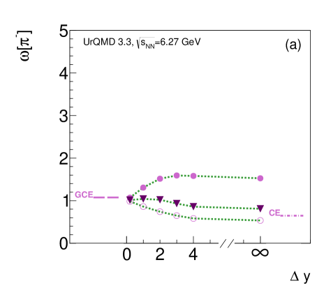
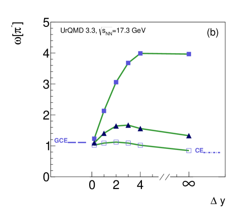
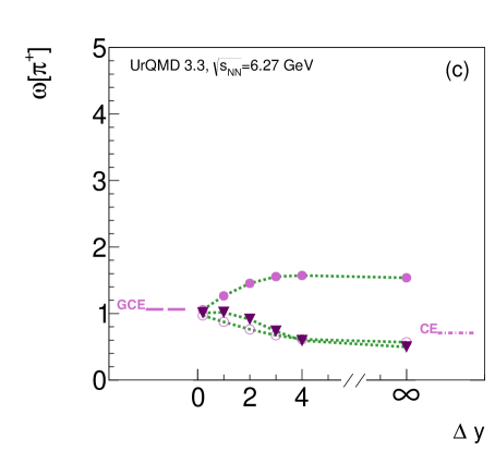
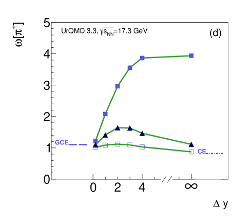
Figure 1: The UrQMD results for the scaled variances $\omega[\pi^{-}]$ and $\omega[\pi^{+}]$ in central Pb+Pb and inelastic $p+p$ collisions for the mid-rapidity windows $\Delta y$, i.e. the center of mass rapidities $y$ of final $\pi^{+}$ and $\pi^{-}$ satisfy the condition $-\Delta Y<y<\Delta Y$. Full circles and squares correspond to the 5% centrality selection and the open ones to the most central Pb+Pb collision events with zero impact parameter $b=0$ fm. Triangles correspond to the UrQMD simulations of inelastic $p+p$ interactions. The collision energies are: $\sqrt{s_{NN}}=6.27$ GeV in (a) and (c), and $\sqrt{s_{NN}}=17.3$ GeV in (b) and (d). The horizontal dashed and dashed-dotted lines show, respectively, the GCE (Table II) and CE (Table IV) results taken at the corresponding $\sqrt{s_{NN}}$.

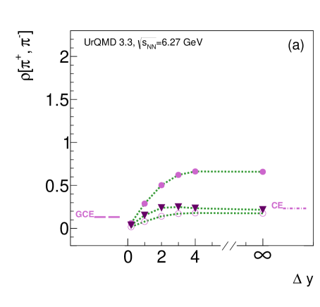
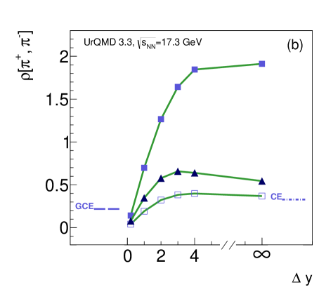
Figure 2: The same as in Fig. 1 but for the correlation parameter $\rho[\pi^{+},\pi^{-}]$.

For the 5% most central Pb+Pb collisions the scaled variance $\omega[\pi^{-}]$, shown in Fig. 1 (a) and (b), increases with $\Delta y$. As seen from Fig. 1 (b), this increase is rather strong at high collision energy: at large $\Delta y$, the value of $\omega[\pi^{-}]$ becomes much larger than the HGM results in both the CE and GCE. The behavior of $\omega[\pi^{+}]$, shown in Fig. 1 (c) and (d), is rather similar to that of $\omega[\pi^{-}]$.

The correlation parameter $\rho[\pi^{+},\pi^{-}]$ is presented in Fig. 2 (a) and (b). Selecting within the UrQMD simulations the most central Pb+Pb collision events with zero impact parameter $b=0$ fm, one finds essentially smaller values of $\omega[\pi^{-}]$, $\omega[\pi^{+}]$ (open symbols in Fig. 1), and $\rho[\pi^{+},\pi^{-}]$. This means that in the 5% centrality bin of Pb+Pb collision events large fluctuations of the number of nucleon participants (i.e., the volume fluctuations) are present. These volume fluctuations produce large additional contributions to the scaled variances of pions and to the correlation parameter $\rho[\pi^{+},\pi^{-}]$. These contributions were presented as the separate terms in Eqs. (14-16). They become more and more important with increasing collision energy. This is due to an increase of the pion number density (or, similarly, the number of pions per participating nucleon) with increasing collision energy. However, one hopes that these volume fluctuations will be canceled out to a large extent when they are combined in the strongly intensive measures. Note also that the UrQMD results for $\omega[\pi^{-}]$, $\omega[\pi^{+}]$, and $\rho[\pi^{+},\pi^{-}]$ in inelastic $p+p$ collisions, shown in Figs. 1 and 2 by triangles, are qualitatively similar to those in Pb+Pb collisions at $b=0$ fm.

The UrQMD results for $\Sigma[\pi^{+},\pi^{-}]$ in Pb+Pb collisions at $\sqrt{s_{NN}}=6.27$ GeV and 17.3 GeV are presented in Fig. 3 (a) and (b), respectively, as a function of the acceptance window $\Delta y$ at mid-rapidity.

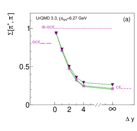
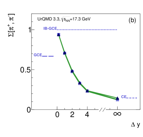
Figure 3: The same as in Figs. 1 and 2 but for $\Sigma[\pi^{+},\pi^{-}]$. The horizontal dotted line shows the IB-GCE result $\Sigma[\pi^{+},\pi^{-}]=1$.

In contrast to the results shown in Figs. 1 and 2, both centrality selections in Pb+Pb collisions (5% centrality bin and $b=0$ fm) lead to very similar results for $\Sigma[\pi^{+},\pi^{-}]$ shown in Fig. 3. This means that the measure $\Sigma[\pi^{+},\pi^{-}]$ has the strongly intensive properties, at least in the UrQMD simulations. The UrQMD results in p+p reactions are close to those in Pb+Pb ones.

The GCE and CE results from Tables 2 and 4 are presented in Figs. 1-3 by the horizontal dashed and dashed-dotted lines, respectively. The UrQMD results for $\Sigma[\pi^{+},\pi^{-}]$, presented in Fig. 3, demonstrate a strong dependence on the size of rapidity window $\Delta y$. At $\Delta y=1$ these results are close to those of the GCE HGM. On the other hand, with increasing $\Delta y$ the role of exact charge conservation becomes more and more important. From Fig. 3, one observes that the UrQMD values of $\Sigma[\pi^{+},\pi^{-}]$ at large $\Delta y$ are close to the CE results.

As seen from Figs. 1 and 2, a similar correspondence between the UrQMD results for $\omega[\pi^{-}]$, $\omega[\pi^{+}]$, and $\rho[\pi^{+},\pi^{-}]$ in Pb+Pb collisions at $b=0$ fm and their GCE and CE values is approximately valid. However, this is not the case for the 5% most central Pb+Pb events. In that centrality bin the volume fluctuations give the dominant contributions to $\omega[\pi^{-}]$, $\omega[\pi^{+}]$, and $\rho[\pi^{+},\pi^{-}]$ for large $\Delta y$.

For very small acceptance, $\Delta y\ll 1$, one expects an approximate validity of the Poisson distribution for any type of the detected particles. Their scaled variances are then close to unity, i.e., $\omega[\pi^{-}]\cong\omega[\pi^{+}]\cong 1$. Particle number correlations, due to both the resonance decays and the global charge conservation, become negligible, i.e., $\rho[\pi^{+},\pi^{-}]\ll 1$. Therefore, at very small $\Delta y$ the IB-GCE results should be valid. These expectations are indeed supported by the UrQMD results at $\Delta y=0.2$ presented in Figs. 1 and 2. Therefore, one expects $\Sigma[\pi^{+},\pi^{-}]\rightarrow 1$ at $\Delta y\rightarrow 0$. This expectation is also valid, as seen from the UrQMD results at $\Delta y=0.2$ presented in Fig. 3.

VI Summary

In this paper we use the strongly intensive measures $\Delta$ and $\Sigma$ and analyze the effects of resonance decays for the particle number fluctuations and correlations. Two examples for which the event by event fluctuations of hadron multiplicities are rather sensitive to the abundances of resonances at the chemical freeze-out are discussed: resonance decays to two positively charged particles, like $\Delta^{++}\rightarrow p+\pi^{+}$, and to $\pi^{+}\pi^{-}$-pair, like $\rho^{0}\rightarrow\pi^{-}+\pi^{+}$. Simple analytical formulation demonstrates that the resonance abundances, which are difficult to be measured by other methods, can be found by measuring the fluctuations and correlations of the numbers of stable hadrons. The grand canonical ensemble calculations within the hadron-resonance gas model support these physical results.

The ultra-relativistic quantum molecular dynamics model is used in Pb+Pb and $p+p$ collisions at the SPS energies to illustrate the role of centrality selection, limited acceptance, and global charge conservation. A crucial importance of the size of the rapidity window for the accepted particles is emphasized. It should be larger than unity for a simultaneous hit into this rapidity window of both correlated hadrons, e.g., $\pi^{+}$ and $\pi^{-}$, from resonance decays. However, if this window of accepted particles is comparable to the whole rapidity interval the restrictions of the exact global charge conservations become important. This is illustrated by the canonical ensemble calculations when the conserved charges are fixed for all microscopic states. The global charge conservation influences the particle number fluctuations and introduces additional correlations between numbers of different particle species. Thus, a connection between the fluctuation measures and the resonance abundances becomes more complicated. The high energy RHIC and LHC accelerators look therefore preferable for these investigations: one can use a large enough rapidity interval (comparing to unity) which will be only a small part of the whole system.