Efficient first-principles calculation of the quantum kinetic energy
and momentum distribution of nuclei

Abstract

Light nuclei at room temperature and below exhibit a kinetic energy which significantly deviates from the predictions of classical statistical mechanics. This quantum kinetic energy is responsible for a wide variety of isotope effects of interest in fields ranging from chemistry to climatology. It also furnishes the second moment of the nuclear momentum distribution, which contains subtle information about the chemical environment and has recently become accessible to deep inelastic neutron scattering experiments. Here we show how, by combining imaginary time path integral dynamics with a carefully designed generalized Langevin equation, it is possible to dramatically reduce the expense of computing the quantum kinetic energy. We also introduce a transient anisotropic Gaussian approximation to the nuclear momentum distribution which can be calculated with negligible additional effort. As an example, we evaluate the structural properties, the quantum kinetic energy, and the nuclear momentum distribution for a first-principles simulation of liquid water.

One of the most commonly adopted approximations in atomistic simulations of materials and chemical compounds is the assumption that atomic nuclei behave as classical particles. Unfortunately, whenever hydrogen or other light nuclei are present and the simulation is performed at or below room temperature, significant deviations from classical behaviour are to be expected. Moreover, many interesting physical phenomena and experimental observables depend directly on the quantum nature of the nuclear motion. This implies that an explicit treatment of nuclear quantum effects (NQE) may not only be desirable to improve the accuracy of the simulation; it can even be essential for comparison with experiments. In particular, the quantum kinetic energy (QKE) underlies all changes in relative free energy associated with isotopic substitution, which are responsible for phenomena as diverse as isotope effects in enzyme catalysis and the fractionation of isotopes between different compounds and phases. The accurate evaluation of NQE therefore has implications for disciplines ranging from chemistry, biochemistry, and materials science to geology, archaeometry, and climatology Westheimer (1961); *cha+89science; *flan-oate91arms; *frie-onei77book; *savi-epst70gca; *gat96areps.

The state-of-the-art method for computing the QKE involves the use of path integral molecular dynamics (PIMD) Parrinello and Rahman (1984). This allows one to systematically converge NQE but introduces an often prohibitive overhead with respect to a simulation with classical nuclei, since one has to compute the energy of many replicas of the physical system. Recently it has been suggested that a generalized Langevin equation (GLE) can be used to model NQE less expensively Ceriotti et al. (2009); Buyukdagli et al. (2008); *damm+09prl, and that systematic convergence can be obtained by combining path integrals (PI) with an appropriate GLE Ceriotti et al. (2011). In the present Letter we generalize this PI+GLE approach in such a way that different quantum mechanical observables, including the QKE, can be obtained at a fraction of the cost of a full PI calculation. We also introduce a convenient “transient anisotropic Gaussian” (TAG) approximation to the nuclear momentum distribution $n(p)$. This significantly simplifies the task of comparing first-principles atomistic modeling with deep inelastic neutron scattering (DINS) Andreani et al. (2005); *pant+08prl; *andr+11cpl; *flam+12jcp – a promising experimental technique which directly probes the quantum nature of light atoms.

Path integral molecular dynamics is based on the isomorphism between the quantum mechanical partition function of a system of $N$ distinguishable particles and the classical partition function of a so-called ring polymer Chandler and Wolynes (1981), described by the Hamiltonian

$$H_{P}\left(\mathbf{p},\mathbf{q}\right)=\sum_{i=0}^{P-1}\frac{1}{2}\mathbf{p}_{i}^{2}+V\left(\mathbf{q}_{i}\right)+\frac{1}{2}\omega_{P}^{2}\left(\mathbf{q}_{i}-\mathbf{q}_{i+1}\right)^{2}.$$ (1)

Here $P$ is the number of replicas (beads) composing the path, $\mathbf{q}_{i}$ and $\mathbf{p}_{i}$ are $3N$-dimensional vectors describing the mass-scaled positions and momenta of the particles in the $i$-th replica, and $V(\mathbf{q}_{i})$ is the physical potential acting on replica $i$. For a simulation at the physical temperature $1/k_{B}\beta$, the harmonic interaction between neighbouring beads is characterized by the frequency $\omega_{P}=P/\beta\hbar$, and the ring polymer Hamiltonian (1) must be sampled at $P$ times the physical temperature.

As the number of replicas is increased, the equilibrium properties computed from the simulation converge to the correct quantum mechanical expectation values. In particular, one can compute the average potential

$$\left<V\right>=\frac{1}{P}\sum_{i=0}^{P-1}\left<V(\mathbf{q}_{i})\right>$$ (2)

and the quantum kinetic energy (using the centroid virial estimator Herman et al. (1982); Ceperley (1995))

$$\left<T\right>=\frac{3N}{2\beta}+\frac{1}{2P}\sum_{i=0}^{P-1}\left<\left(\mathbf{q}_{i}-\bar{\mathbf{q}}\right)\cdot\nabla V\left(\mathbf{q}_{i}\right)\right>,$$ (3)

where $\bar{\mathbf{q}}=\sum_{i}\mathbf{q}_{i}/P$ is the centroid of the ring polymer. The convergence of the averages (2) and (3) to the quantum expectation values for a system whose fastest normal mode has frequency $\omega_{\rm max}$ requires a number of replicas of the order of $\beta\hbar\omega_{\rm max}$, making the PI approach very demanding when simulations are performed at low temperature, or in the presence of stiff vibrations.

It has recently been shown that this overhead can be removed by using correlated noise to construct a tailored, non-equilibrium Langevin dynamics that mimics NQE using a single replica Ceriotti et al. (2009). This approach can be made exact in the harmonic limit, without requiring explicit knowledge of the Hessian, but it is inherently approximate in any real system containing anharmonicities. To address this shortcoming, one can combine correlated noise with PIMD Ceriotti et al. (2011). In this PI+GLE approach, each replica is subject to an independent instance of the same GLE thermostat, which is designed in such a way that the expectation value $\left<V\right>$ is exact for any number of replicas in the harmonic limit. Convergence is approached systematically, such that the computational effort required to obtain structural properties is reduced by a factor of 4 or more relative to PIMD Ceriotti et al. (2011).

Note, however, that while the average potential (2) only depends on the positions of individual beads, the kinetic energy (3) involves their centroid $\bar{\bf q}$, and therefore depends on cross-correlations between the coordinates of different beads. The PI+GLE method described in Ref. Ceriotti et al. (2011) does not address the convergence of these correlations, and therefore $\left<T\right>$ is not guaranteed to be exact in the harmonic limit. As a result, the kinetic energy converges more slowly than the potential energy, requiring about twice the number of replicas to reach the same level of accuracy. Fortunately, it is relatively simple to improve PI+GLE to also manipulate bead-bead correlations. It is in fact sufficient to apply different GLE thermostats to the different normal modes of the ring polymer. The desired correlations can then be enforced in the harmonic limit, by separately tuning the parameters of the various thermostats.

This idea is readily applied to the problem of designing a “PIGLET” method, which converges $\left<T\right>$ just as rapidly as $\left<V\right>$ . Evaluating (2) and (3) for a one-dimensional harmonic oscillator of frequency $\omega$ yields

$$\begin{split}\left<T\right>=&\frac{1}{2\beta}+\frac{1}{2P}\omega^{2}\sum_{i=0}^{P-1}\left<q_{i}^{2}\right>-\frac{1}{2}\omega^{2}\left<\bar{q}^{2}\right>=\\ =&\left<V\right>+\frac{1}{2\beta}-\frac{1}{2}\omega^{2}\left<\bar{q}^{2}\right>.\end{split}$$ (4)

Therefore, in order to enforce the quantum conditions

$$\left<V\right>=\left<T\right>=\frac{\hbar\omega}{4}\coth{\beta\hbar\omega\over 2},$$ (5)

one sees that the centroid must be distributed classically, leaving the fluctuations of the individual beads to impose the quantum statistics. The simplest way to ensure this is to apply a classical thermostat to the centroid coordinate, and the same non-equilibrium GLE to all the internal modes of the ring polymer. This second thermostat must be designed to enforce the correct quantum fluctuations on each normal mode, in accordance with (5). The desired frequency-dependence of the thermostat temperature can be obtained by solving a functional equation analogous to Eq. (16) in Ref. Ceriotti et al. (2011). Parameters for such a GLE thermostat have been generated using the fitting procedure described in Ref. Ceriotti et al. (2010), and may be found in the supplementary material EPA or downloaded from gle .

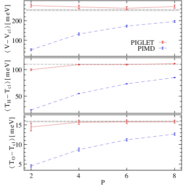
Figure 1: Per-molecule quantum contribution to the potential energy and per-atom quantum kinetic energy plotted as a function of the number of PI replicas. The convergence of conventional PIMD (blue points) is compared with the present method (red points). Data points are reported with $2\sigma$ error bars, which have been inferred from longer simulations using an empirical water model EPA . In each panel, the dashed line corresponds to the average computed from a $32$-bead PIMD reference calculation, and the shaded area to a $2\sigma$ confidence interval.

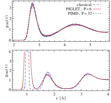
Figure 2: Radial distribution functions for the O–O (upper panel) and O–H (lower panel) pairs. Results from classical MD are reported in blue, results from a PIGLET simulation with 6 beads are reported in red. A reference calculation with conventional PIMD using 32 beads is reported as a black, dashed line. Statistical confidence intervals are represented as shaded areas and have been inferred from longer simulations using an empirical water model EPA .

To illustrate the potential of this PIGLET method, we have performed a simulation of liquid water modelled using density functional theory, as implemented in the CP2K code VandeVondele et al. (2005); *goed+96prb. We used the BLYP exchange-correlation functional Becke (1988); *lee+88prb, and the same well-established simulation details as described in Ref. Hassanali et al. (2011). We performed simulations of a box of 64 water molecules at a temperature of $300$ K and the experimental density. We used a time step of $0.5$ fs, and each simulation was $15$ ps long with the first $3$ ps discarded for equilibration. 32-bead PIMD simulations required a shorter time step of $0.25$ fs, and were only $7.5$ ps long.

Figure 1 demonstrates the fast convergence of $\left<V\right>$ and $\left<T\right>$, both of which reach a level of accuracy within the statistical error of a standard $32$-bead PIMD simulation using just 6 beads. This dramatic reduction in the computational effort required to compute the QKE would for instance make it possible to evaluate isotope fractionation between the liquid and the gas phases of water by first-principles simulations. In this context, the delicate balance between the competing quantum effects which characterise the behaviour of water Habershon et al. (2009); Li et al. (2011); Markland and Berne (2012) would provide a sensitive benchmark for the relative merits of different exchange-correlation functionals. Furthermore, the increased efficiency in computing the QKE does not come at the expense of the accuracy of structural properties: in Figure 2 we demonstrate that the O-H and O-O radial distribution functions computed with PIGLET using 6 beads also agree with those from a 32-bead PIMD simulation to within the statistical accuracy.

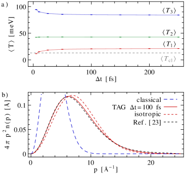
Figure 3: Panel (a) shows the principal values of the TAG kinetic energy tensor as a function of the moving average window width $\Delta t$, for a 6-bead PIGLET simulation of liquid water at $300$ K. Panel (b) compares the classical $n(p)$ for a proton at $300$ K (blue curve) with the TAG $n(p)$ obtained using $\Delta t=100$ fs. Other values of $\Delta t$ in the range $100<\Delta t<500$ fs give the same result to graphical accuracy. Note the nearly-perfect agreement with the open-path $n(p)$ from Ref. Morrone and Car (2008) (black dashed line), which is in turn in very good agreement with experimental data Reiter et al. (2004); *giul+11prl; Morrone and Car (2008). The TAG gives a significant improvement over an isotropic Gaussian approximation (red dashed line).

The quantum kinetic energy is also directly related to the second moment of the distribution of particle momentum $n(p)$, which can be measured in DINS experiments. The nuclear momentum distribution, however, contains more information about the chemical environment of the nucleus than the kinetic energy alone. In order to access $n(p)$ computationally, the state-of-the-art technique involves performing an open path or displaced path PIMD simulation, both of which are even more complex and computationally demanding than conventional PIMD Lin et al. (2010).

Fortunately, it turns out that $n(p)$ can often be modelled very accurately as resulting from the spherical average of an anisotropic three-dimensional Gaussian distribution Pantalei et al. (2008); Lin et al. (2011). For an individual atom in a rigid environment, one could imagine constructing such a distribution by computing the principal components of its kinetic energy tensor, the virial estimator for which is

$$T_{\alpha\beta}=\frac{\delta_{\alpha\beta}}{2\beta}+\frac{1}{4P}\sum_{i}\left[\left(q_{i\alpha}-\bar{q}_{\alpha}\right)\frac{\partial V}{\partial q_{i\beta}}+\left(q_{i\beta}-\bar{q}_{\beta}\right)\frac{\partial V}{\partial q_{i\alpha}}\right].$$ (6)

Here $q_{i\alpha}$ indicates Cartesian component $\alpha$ of the position of the $i$-th replica of the atom in the ring polymer.

If one were to compute the average of (6) for an atom in liquid water, however, an isotropic tensor would be obtained, because of the ever-changing orientation of the water molecules. On the other hand, the fact that the experimental $n(p)$ agrees with an anisotropic Gaussian model suggests that instantaneously each atom has a quasi-Gaussian momentum distribution, albeit in a dynamic, transient frame of reference. This idea suggests a very simple approximation to $n(p)$ based on a moving average of the kinetic energy tensor:

$$T_{\alpha\beta}(t;\Delta t)=\frac{1}{\Delta t}\int_{t-\Delta t}^{t+\Delta t}T_{\alpha\beta}(t^{\prime})\left(1-\frac{\left|t-t^{\prime}\right|}{\Delta t}\right)\mathrm{d}t^{\prime}.$$ (7)

Suppose that we evaluate the eigenvalues $T_{\gamma}\left(t;\Delta t\right)$ of this tensor (sorted in increasing order) at each instant $t$, and compute their averages $\left<T_{\gamma}(\Delta t)\right>$ along the trajectory. Then these averages can be used to define a “transient anisotropic Gaussian” (TAG) approximation to $n(p)$, with $\left<p_{\gamma}^{2}\right>=2\left<T_{\gamma}(\Delta t)\right>$ for $\gamma=1,2,3$ .

As shown in Figure 3(a), all three $\left<T_{\gamma}(\Delta t)\right>$ converge to plateau values after a characteristic time interval $\Delta t$ – the time needed to establish the principal axes of the TAG. On a much longer time scale, if the atom in question experiences many different transient environments, one would expect all three $\left<T_{\gamma}(\Delta t)\right>$ to drift, eventually approaching $\left<T\right>/3$ in an isotropic system such as a liquid. In Figure 3(b) we show that the spherical average of the TAG generated with the plateau values of $\left<T_{\gamma}(\Delta t)\right>$ almost perfectly matches the results obtained with heroic effort by Morrone and Car Morrone and Car (2008) using an open path integral simulation, and differs significantly from the $n(p)$ constructed from an isotropic Gaussian with $\left<p^{2}\right>=2\left<T\right>$.

The TAG approximation shares some similarities with the Gaussian approximation to the open path distribution introduced in Ref. Lin et al. (2011), and with the idea of computing the components of the kinetic energy along a set of orthogonal vectors anchored to the molecular axes of individual water molecules Markland and Berne (2012). Some of the advantages of the TAG approach are that: (1) it is not necessary to open any paths, so there is no additional sampling overhead compared with a conventional PIMD simulation; (2) since all paths remain closed, one can increase the statistical efficiency by averaging the computed $n(p)$ over all equivalent atoms; (3) it is not restricted to crystals or to systems with identifiable molecular axes – the local frame of reference of each atom does not have to be specified in advance but is determined automatically; and (4) it comes with an internal sanity check, since one can verify the existence of a transient local environment by checking that all three $\left<T_{\gamma}(\Delta t)\right>$ reach well-defined plateaus.

(meV)	$\left<T\right>$	(Exp; Temp.)	$\left<T_{1}\right>$	$\left<T_{2}\right>$	$\left<T_{3}\right>$
H (H2O)	$148.2$	(145; 296K)	20.6	42.8	84.7
D (D2O)	$110.1$	(106$\pm$5; 292K)	16.4	31.4	62.4
O (H2O)	$54.6$		14.4	18.3	21.8
O (D2O)	$58.1$		14.5	19.6	24.0

Table 1: Per-atom QKE and its TAG components in simulations of light and heavy water at $300$ K, computed using $\Delta t=100$ fs. NQE were described by the PIGLET method with $6$ beads. All the statistical errors are smaller than $0.1$ meV. Where available, experimental results at a similar temperature are reported in parentheses Reiter et al. (2004); *giul+11prl.

The TAG $n(p)$ is also sufficiently accurate to reveal some rather subtle effects, which may be detectable in DINS experiments that are currently underway Senesi et al. (2012). In a comparative study of light and heavy water, one finds that while the D nuclei have a lower QKE in D₂O than the H nuclei in H₂O, the oxygen nuclei actually have a higher QKE in D₂O than in H₂O. This observation can be rationalised in terms of a reduced mass effect, whereby the O nucleus in heavy water shares a higher fraction of the intra-molecular zero-point energy than the oxygen in light water. As shown in Table 1, the effect is clearly captured by the TAG approximation. One of the components of the O momentum distribution, orthogonal to the plane of the molecule, is almost unaffected by the isotope substitution, while the components which contribute to the intra-molecular vibrations possess a higher QKE in D₂O than in H₂O.

The methods we have introduced in this Letter clearly simplify the task of computing properties related the quantum nature of light nuclei, potentially enabling comparison with experimental observations in more complex cases than have hitherto been possible. The resulting interplay between theory and experiment will be essential to unravel the competing quantum effects that govern the behaviour of water and other hydrogen-bonded systems Li et al. (2011).

This work was supported by the Royal Society, the Swiss National Science Foundation, the Wolfson Foundation, and the EU Marie Curie IEF n. PIEF-GA-2010-272402. Computer time from the University of Lugano is gratefully acknowledged.

References

- Westheimer (1961) F. H. Westheimer, Chemical Reviews 61, 265 (1961).
- Cha et al. (1989) Y. Cha, C. J. Murray, and J. P. Klinman, Science 243, 1325 (1989).
- Flanagan and Oates (1991) T. B. Flanagan and W. A. Oates, Annual Review of Materials Science 21, 269 (1991).
- Friedman and O’Neil (1977) I. Friedman and J. R. O’Neil, Compilation of stable isotope fractionation factors of geochemical interest, Vol. 440 (USGPO, 1977).
- Savin and Epstein (1970) S. M. Savin and S. Epstein, Geochimica et Cosmochimica Acta 34, 25 (1970).
- Gat (1996) J. R. Gat, Annual Review of Earth and Planetary Sciences 24, 225 (1996).
- Parrinello and Rahman (1984) M. Parrinello and A. Rahman, J. Chem. Phys. 80, 860 (1984).
- Ceriotti et al. (2009) M. Ceriotti, G. Bussi, and M. Parrinello, Phys. Rev. Lett. 103, 030603 (2009).
- Buyukdagli et al. (2008) S. Buyukdagli, A. V. Savin, and B. Hu, Phys. Rev. E 78, 066702 (2008).
- Dammak et al. (2009) H. Dammak, Y. Chalopin, M. Laroche, M. Hayoun, and J.-J. Greffet, Phys. Rev. Lett. 103, 190601 (2009).
- Ceriotti et al. (2011) M. Ceriotti, D. E. Manolopoulos, and M. Parrinello, J. Chem. Phys. 134, 084104 (2011).
- Andreani et al. (2005) C. Andreani, D. Colognesi, J. Mayers, G. F. Reiter, and R. Senesi, Adv. Phys. 54, 377 (2005).
- Pantalei et al. (2008) C. Pantalei, A. Pietropaolo, R. Senesi, S. Imberti, C. Andreani, J. Mayers, C. Burnham, and G. Reiter, Phys. Rev. Lett. 100, 177801 (2008).
- Andreani et al. (2011) C. Andreani, D. Colognesi, A. Pietropaolo, and R. Senesi, Chem. Phys. Lett. 518, 1 (2011).
- Flammini et al. (2012) D. Flammini, A. Petropaolo, R. Senesi, C. Andreani, F. McBride, A. Hodgson, M. Adams, L. Lin, and R. Car, J. Chem. Phys. 136, 024504 (2012).
- Chandler and Wolynes (1981) D. Chandler and P. G. Wolynes, J. Chem. Phys. 74, 4078 (1981).
- Herman et al. (1982) M. F. Herman, E. J. Bruskin, and B. J. Berne, J. Chem. Phys. 76, 5150 (1982).
- Ceperley (1995) D. M. Ceperley, Rev. Mod. Phys. 67, 279 (1995).
- Note (1) Note that this approach could easily be extended to manipulate the bead-bead correlations in a PI+GLE simulation even further, so as to accelerate the convergence of other PI estimators – for example those used to compute imaginary-time correlation functions.
- Ceriotti et al. (2010) M. Ceriotti, G. Bussi, and M. Parrinello, Journal of Chemical Theory and Computation 6, 1170 (2010).
- (21) See supplementary material at [URL] for the GLE parameters used, and an extensive analysis of statistical and systematic errors based on an empirical force field.
- (22) http://gle4md.berlios.de.
- VandeVondele et al. (2005) J. VandeVondele, M. Krack, F. Mohamed, M. Parrinello, T. Chassaing, and J. Hutter, Comp. Phys. Comm. 167, 103 (2005).
- Goedecker et al. (1996) S. Goedecker, M. Teter, and J. Hutter, Phys. Rev. B 54, 1703 (1996).
- Becke (1988) A. D. Becke, Phys. Rev. A 38, 3098 (1988).
- Lee et al. (1988) C. Lee, W. Yang, and R. G. Parr, Phys. Rev. B 37, 785 (1988).
- Hassanali et al. (2011) A. Hassanali, M. K. Prakash, H. Eshet, and M. Parrinello, Proc. Natl. Acad. Sci. USA 108, 20410 (2011).
- Habershon et al. (2009) S. Habershon, T. E. Markland, and D. E. Manolopoulos, J. Chem. Phys. 131, 024501 (2009).
- Li et al. (2011) X. Z. Li, B. Walker, and A. Michaelides, Proc. Natl. Acad. Sci. USA 108, 6369 (2011).
- Markland and Berne (2012) T. E. Markland and B. J. Berne, Proc. Natl. Acad. Sci. USA (2012).
- Morrone and Car (2008) J. A. Morrone and R. Car, Phys. Rev. Lett. 101, 017801 (2008).
- Reiter et al. (2004) G. Reiter, J. C. Li, J. Mayers, T. Abdul-Redah, and P. Platzman, Braz. J. Phys. 34, 142 (2004).
- Giuliani et al. (2011) A. Giuliani, F. Bruni, M. A. Ricci, and M. A. Adams, Phys. Rev. Lett. 106, 255502 (2011).
- Lin et al. (2010) L. Lin, J. A. Morrone, R. Car, and M. Parrinello, Phys. Rev. Lett. 105, 110602 (2010).
- Lin et al. (2011) L. Lin, J. A. Morrone, R. Car, and M. Parrinello, Phys. Rev. B 83, 220302 (2011).
- Note (2) Note that by construction, so that the computed within this TAG approximation will automatically be consistent with the total QKE.
- Note (3) If the of individual particles were to exhibit significant non-Gaussian behaviour, neither of these techniques nor the TAG approach would be a substitute for a much more demanding open path simulation.
- Senesi et al. (2012) R. Senesi, C. Andreani, et al., (2012), in preparation.