Optimal quantum control of Bose-Einstein condensates in magnetic microtraps: Comparison of GRAPE and Krotov optimization schemes

Abstract

We study optimal quantum control of the dynamics of trapped Bose-Einstein condensates: The targets are to split a condensate, residing initially in a single well, into a double well, without inducing excitation; and to excite a condensate from the ground to the first excited state of a single well. The condensate is described in the mean-field approximation of the Gross-Pitaevskii equation. We compare two optimization approaches in terms of their performance and ease of use, namely gradient ascent pulse engineering (GRAPE) and Krotov’s method. Both approaches are derived from the variational principle but differ in the way the control is updated, additional costs are accounted for, and second order derivative information can be included. We find that GRAPE produces smoother control fields and works in a black-box manner, whereas Krotov with a suitably chosen step size parameter converges faster but can produce sharp features in the control fields.

I Introduction

Controlling complex quantum dynamics is a recurring theme in many different areas of AMO physics and physical chemistry. Recent examples include quantum state preparation Sayrin et al. (2011); Bücker et al. (2011), interferometry van Frank et al. (2014) and imaging Lapert et al. (2012); Häberle et al. (2013), or reaction control Rybak et al. (2011); González-Férez and Koch (2012). The central idea of quantum control is to employ external fields to steer the dynamics in a desired way Rice and Zhao (2000); Brumer and Shapiro (2003). The fields that realize the desired dynamics can be determined by optimal control theory (OCT) Tannor et al. (1992); Werschnik and Gross (2007). An expectation value that encodes the target is then taken to be a functional of the external field which is minimized or maximized. The target can be simply a desired final state Tannor et al. (1992), or a unitary operator Palao and Kosloff (2002), a prescribed value of energy or position Doria et al. (2011), or an experimental signal such as a pump-probe trace Kaiser and May (2004).

The algorithms that can be employed for optimizing the target functional broadly fall into two categories – those where changes in the field are determined solely by evaluating the functional, such as simplex algorithms Doria et al. (2011); Caneva et al. (2011), and those that utilize derivative information, such as Krotov’s method Konnov and Krotov (1999); Sklarz and Tannor (2002) or gradient ascent pulse engineering (GRAPE) Khaneja et al. (2005), possibly combined with quasi-Newton methods Machnes et al. (2011); Eitan et al. (2012). The solutions that one obtains typically do not only depend on the target functional but also on the specific algorithm that is employed and the initial guess field. This is due to the fact that numerical optimization is always a local search which may find one of possibly many optimal solutions or get stuck in a local extremum. It is thus important to understand which features of an optimal control solution are due to the optimization procedure and which reflect truly physical properties of the quantum system.

For example, when seeking to identify, by use of optimal control theory, the quantum speed limit, i.e., the shortest possible time in which a quantum operation can be carried out Caneva et al. (2009), the answer should be independent of the algorithm. Moreover, in view of employing calculated solutions in an experiment, conditions such as limited power, limited time resolution, or limited bandwidth need to be met. The way in which the various optimization approaches can accommodate such requirements differ greatly.

Here, we study control of a Bose-Einstein condensate in a magnetic microtrap, comparing several variants of a GRAPE-type algorithm Hohenester et al. (2007); Hohenester (2014) with Krotov’s method Konnov and Krotov (1999); Sklarz and Tannor (2002); Reich et al. (2012). We consider two targets – splitting the condensate, which resides initially in the ground state of a single well, into a double well, without inducing excitation, and exciting the condensate from the ground to the first excited state of a single well. The latter is important for stimulated processes in matter waves, whereas the former presents a crucial step in interferometry Shin et al. (2004); Schumm et al. (2005); Grond et al. (2010). A challenging aspect of controlling a condensate is the non-linearity of the equation of motion which can compromise or even prevent convergence of the optimization Sklarz and Tannor (2002). The two methods tackle this problem in different ways, GRAPE by computing the search direction for new control fields within the framework of Lagrange parameters and submitting the optimal control search to generic minimization routines Peirce et al. (1988); Hohenester et al. (2007), Krotov’s method by accounting for the non-linearity of the equations of motion in the monotonicity conditions when constructing the algorithm Konnov and Krotov (1999); Sklarz and Tannor (2002); Reich et al. (2012). Furthermore, the methods differ in the way in which additional requirements such as smoothness of the control can be accounted for. We compare the two optimization approaches with respect to the solutions they yield as well as their performance, and ease of use. Our study extends an earlier comparison of GRAPE-type algorithms with Krotov’s method Machnes et al. (2011) that was concerned with the linear Schrödinger equation and with finite-size (spin-type) quantum systems.

Our paper is organized as follows: After introducing the equation of motion for the condensate dynamics together with the control targets in Sec. II, we briefly review the two optimization schemes in Sec. III. Section IV presents our results for wavefunction splitting and shaking. Moreover, we investigate the influence of the nonlinearity, the performance of the two algorithms, and the smoothness of the optimized control in Secs. IV.2 to IV.4. Our conclusions are presented in Sec. V.

II Model and Optimization Problem

In this paper we consider a quasi-1D condensate residing in a magnetic confinement potential $V(x,\lambda(t))$ that can be controlled by some external control parameter $\lambda(t)$ Hohenester et al. (2007); Bücker et al. (2011, 2013); Hohenester (2014). We describe the condensate dynamics within the mean-field framework of the Gross-Pitaevskii equation, where $\psi(x,t)$ is the condensate wavefunction, normalized to one, whose time evolution is governed by Leggett (2001) ($\hbar=1$)

$$i\frac{\partial\psi(x,t)}{\partial t}=\Bigl{(}-\frac{1}{2M}\frac{\partial^{2}}{\partial x^{2}}+V(x,\lambda(t))+\kappa\bigl{|}\psi(x,t)\bigr{|}^{2}\Bigr{)}\psi(x,t)\,.$$ (1)

The first term on the right-hand side is the operator for the kinetic energy, the second one is the confinement potential, and the last term is the nonlinear atom-atom interaction in the mean field approximation. $M$ is the atom mass and $\kappa$ is the strength of the nonlinear atom-atom interactions, which is related to the effective one-dimensional interaction strength $U_{0}$ and the number of atoms $N$ through $\kappa=U_{0}(N-1)$ Grond et al. (2009).

We can now formulate our optimal control problem. Suppose that the condensate is initially described by the wavefunction $\psi(x,0)=\psi_{0}(x)$ and the potential is varied in the time interval $[0,T]$. We are now seeking for an optimal time variation of $\lambda(t)$ that brings the terminal wavefunction $\psi(x,T)$ as close as possible to a desired wavefunction $\psi_{d}(x)$. To rate the success for a given control, we introduce the cost function

$$J_{T}(\psi(T))=\frac{1}{2}\left[1-\left|\left<\psi_{d}|\psi(T)\right>\right|^{2}\right]\,,$$ (2)

which becomes zero when the terminal wavefunction matches the desired one up to an arbitrary phase. Optimal control theory aims at a $\lambda_{\rm OCT}(t)$ that minimizes Eq. (2).

III Optimization Methods

Algorithm	line search	free parameter	deriv	penalty	penalty equation	update	update equation
GRAPE grad L2	yes	$\gamma$	1	$\dot{\lambda}^{2}$	Eq. (3)	concurrent	Eq. (6)
GRAPE grad H1	yes	$\gamma$	1	$\dot{\lambda}^{2}$	Eq. (3)	concurrent	Eq. (7)
GRAPE BFGS L2	yes	$\gamma$	2	$\dot{\lambda}^{2}$	Eq. (3)	concurrent	Eq. (6)
GRAPE BFGS H1	yes	$\gamma$	2	$\dot{\lambda}^{2}$	Eq. (3)	concurrent	Eq. (7)
Krotov	no	$k$	1	$(\Delta\lambda)^{2}$	Eq. (9)	sequential	Eq. (10)
KBFGS	no	$k$	2	$(\Delta\lambda)^{2}$	Eq. (9)	sequential	Eq. (38) of Ref. Eitan et al. (2012)

Table 1: Optimization approaches used in this paper. For each algorithm, we specify whether a line search is used; what free parameter is available to influence the optimization; the order of the derivative for the determination of the new control parameter; the penalty term that is added to Eq. (2), with $\Delta\lambda=\lambda-\lambda_{\rm ref}$; the equation for the cost function; the type of the update of the control; and the update equation used in our simulations.

In this paper, we apply two different optimal control approaches, namely a gradient ascent pulse engineering (GRAPE) scheme Khaneja et al. (2005) and Krotov’s method Konnov and Krotov (1999); Sklarz and Tannor (2002); Reich et al. (2012), which will be discussed separately below. An overview of the control approaches is given in Table 1.

III.1 GRAPE: Functional and Optimization Scheme

The GRAPE scheme for Bose-Einstein condensates has been presented in detail elsewhere Hohenester et al. (2007); Bücker et al. (2013); Jäger and Hohenester (2013); Hohenester (2014), for this reason we only briefly introduce the working equations. Experimentally, strong variations of the control parameter are difficult to achieve. Therefore, we add to the cost function an additional term Hohenester et al. (2007); Borzi and Hohenester (2008); von Winckel and Borzi (2008),

$$J(\psi(T),\lambda)=J_{T}(\psi(T))+\frac{\gamma}{2}\int_{0}^{T}[\dot{\lambda}(t)]^{2}dt\,.$$ (3)

Mathematically, the additional term penalizes strong variations of the control parameter and is needed to make the OCT problem well-posed Hohenester et al. (2007); Borzi and Hohenester (2008); von Winckel and Borzi (2008). Through $\gamma$ it is possible to weight the relative importance of wavefunction matching and control smoothness. Below we will set $\gamma\ll 1$ such that $J$ is dominated by the terminal cost $J_{T}$.

In order to bring the system from the initial state $\psi_{0}$ to the terminal state $\psi(T)$ we have to fulfill the Gross-Pitaevskii equation, which enters as a constraint in our optimization problem. The constrained optimization problem can be turned into an unconstrained one by means of Lagrange multipliers $p(x,t)$, whose time evolution is governed by Hohenester et al. (2007)

$$i\dot{p}=\left(-\frac{1}{2M}\frac{\partial^{2}}{\partial x^{2}}+V(x,\lambda(t))+2\kappa|\psi|^{2}\right)p+\kappa\psi^{2}p^{*}\,,$$ (4)

subject to the terminal condition $p(T)=i\langle\psi_{d}|\psi(T)\rangle\psi_{d}$. The optimal control problem is then composed of the Gross-Pitaevskii equation (1) and Eq. (4), which must be fulfilled simultaneously together with Hohenester et al. (2007)

$$\gamma\ddot{\lambda}=-\mathfrak{Re}\bigl{<}p\bigr{|}\frac{\partial V}{\partial\lambda}\bigl{|}\psi\bigr{>}$$ (5)

for the optimal control. This expression differs from standard GRAPE Khaneja et al. (2005) and results from minimizing changes in the control, cf. Eq. (3).

This set of equations can be also employed for a non-optimal control where Eq. (5) is not fulfilled. In this case Eq. (1) is solved forwards in time and Eq. (4) backwards in time, and the search direction $\nabla_{\lambda}J$ for an improved control is calculated from one of the equations Hohenester et al. (2007); von Winckel and Borzi (2008); Hohenester (2014)

$$\nabla_{\lambda}J\phantom{]}\!\! = \!\!-\gamma\ddot{\lambda}-\mathfrak{Re}\,\bigl{<}p\bigr{|}\frac{\partial V}{\partial\lambda}\bigl{|}\psi\bigr{>}\,\,\,\mbox{for $L^{2}$ norm}\qquad$$ (6)

$$-\frac{d^{2}}{dt^{2}}\bigl{[}\nabla_{\lambda}J\bigr{]}\!\! = \!\!-\gamma\ddot{\lambda}-\mathfrak{Re}\,\bigl{<}p\bigr{|}\frac{\partial V}{\partial\lambda}\bigl{|}\psi\bigr{>}\,\,\,\mbox{for $H^{1}$ norm.}\qquad$$ (7)

These two expressions are obtained by interpreting, on the right hand side of Eq. (3), the integral $\int_{0}^{T}[\dot{\lambda}]^{2}\,dt=\langle\dot{\lambda},\dot{\lambda}\rangle_{L^{2}}=\langle\lambda,\lambda\rangle_{H^{1}}$ in terms of an $L^{2}$ or $H^{1}$ norm von Winckel and Borzi (2008); Grond et al. (2009). The $H^{1}$ norm implies that one additionally has to solve a Poisson equation, see the derivative operator on the left hand side of Eq. (7). This generally results in a much smoother time dependence of the control parameters while the additional numerical effort for solving the Poisson equation is negligible. As for an optimal control, both Eqs. (6) and (7) yield $\nabla_{\lambda}J=0$.

Here we solve the optimal control equations using the Matlab toolbox octbec Hohenester (2014). The ground and desired states of the Gross-Pitaevskii equation are computed using the optimal damping algorithm Dion and Cances (2007); Hohenester (2014). The control parameters are obtained iteratively using either a conjugate gradient method (GRAPE grad), which only uses first order information, or a quasi-Newton BFGS scheme Bertsekas (1999) (GRAPE BFGS), which also takes into account second-order information via an approximated Hessian. In both cases, the optimization employs a line search to determine the optimal step size in the direction of a given gradient. The pulse update is calculated for all time points simultaneously, making the GRAPE schemes concurrent.

III.2 Krotov’s method: Functional and Optimization scheme

Krotov’s method Konnov and Krotov (1999) provides an alternative optimal control implementation. The main idea is to add to Eq. (2) a vanishing term Konnov and Krotov (1999); Sklarz and Tannor (2002); Reich et al. (2012), which is chosen such that the minimum of the new function is also a minimum of $J$. However, for non-optimal $\lambda(t)$ one can devise a scheme that always gives a new control corresponding to a lower cost function. Thus, Krotov’s method leads to a monotonically convergent optimization algorithm that is expected to exhibit much faster convergence.

Our implementation closely follows Refs. Sklarz and Tannor (2002); Reich et al. (2012); Eitan et al. (2012). Specifically, the cost reads

$$J(\psi(T),\lambda)=J_{T}(\psi(T))+\int_{0}^{T}\frac{[\lambda(t)-\lambda_{\rm ref}(t)]^{2}}{S(t)}dt\,,$$ (8)

where the reference field $\lambda_{\rm ref}(t)$ is typically chosen to be the control from the previous iteration Palao and Kosloff (2003). The second term in Eq. (8) penalizes changes in the control from one iteration to the next, and ensures that as an optimum is approached the value of the functional is increasingly determined by only $J_{T}$. $S(t)=ks(t)$ is a shape function that controls the turning on and off of the control fields, $k$ is a step size parameter, and $s(t)\in[0,1]$ is bound between $0$ and $1$.

Let $\psi^{(i)}(t)$ and $\lambda^{(i)}(t)$ denote the wavefunction and control parameter, respectively, in the $i$th iteration of the optimal control loop. To get started, we first solve for an initial guess $\lambda^{(0)}(t)$ the Gross-Pitaevskii equation (1) and the adjoint equation (4) for the co-state $p(t)$, which is backward-propagated in time with the same terminal condition as in GRAPE, in order to obtain $\psi^{(0)}(t)$ and $p^{(0)}(t)$. In the next step, we solve the Gross-Pitaevskii equation simultaneously with the equation for the new control field

$$\lambda^{(i+1)}(t)=\lambda^{(i)}(t)+S(t)\mathfrak{Re}\,\Braket{p^{(i)}(t)}{\left[\frac{\partial V}{\partial\lambda}\right]_{\lambda^{(i+1)}(t)}}{\psi^{(i+1)}(t)}+\mathfrak{Re}\,\frac{\sigma(t)}{2i}\Braket{\Delta\psi(t)}{\left[\frac{\partial V}{\partial\lambda}\right]_{\lambda^{(i+1)}(t)}}{\psi^{(i+1)}(t)}\,,$$ (9)

where $\psi^{(i+1)}(t)$ is obtained by propagating $\psi(t=0)$ forward in time using the updated pulse.  The fact that $\psi^{(i+1)}(t)$ appears on the right hand side of the update equation implies that the update at a given time $t$ depends on the updates at all earlier times, making Krotov’s method sequential. This type of update makes it non-straightforward to include a cost term on the derivative of the control as in Eq. (3), since the derivative at a given time $t$ requires knowledge of past and future values of $\psi(t)$.

The last term in Eq. (9) with $\Delta\psi(t)=\psi^{(i+1)}(t)-\psi^{(i)}(t)$ is generally needed to ensure convergence in presence of the nonlinear mean-field term $\kappa|\psi(t)|^{2}$ of the Gross-Pitaevskii equation. Convergence is achieved through a proper choice of $\sigma(t)$ Sklarz and Tannor (2002); Reich et al. (2012). In this work we neglect this additional contribution for simplicity, as it is of only minor importance for the moderate $\kappa$ values of our present concern.

Figure 1: (Color online) Wavefunction splitting through the transformation of the confinement potential from a single to a double well. (a) The solid lines report the control parameters $\lambda(t)$ for the GRAPE and Krotov optimizations, respectively. The potential is held constant after the terminal time $T=2$ ms. The dashed line shows the shape function $s(t)$ of Eq. (8) used in our version of Krotov’s method, scaled by a factor of $0.4$ for better visibility. (b,c) Density plots of the condensate density $n(x,t)=|\psi(x,t)|^{2}$ during the splitting. The solid lines show the confinement potentials at three selected times and the time variation of the potential minima. (d,e) Terminal (solid lines) and desired (dashed lines) densities, which are indistinguishable. In the optimization we set $\gamma=10^{-6}$ and $k=10^{-3}$.

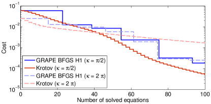
Figure 2: (Color online) Cost function versus number of solved equations (either Gross-Pitaevskii or adjoint equation) for GRAPE and Krotov. For GRAPE one optimization iteration consists of numerous solutions of the Gross-Pitaevskii equation (1) during a line search, which are followed by a solution of the adjoint equation (4) once a minimum is found, to obtain a new search direction $\nabla_{\lambda}J$. For Krotov one optimization iteration consists of a Gross-Pitaevskii solution, subject to Eq. (10), and a subsequent solution of the adjoint equation (4). In our simulations we use $k=10^{-3}$. The dashed lines report results of simulations with a larger nonlinearity $\kappa/\hbar=2\pi\times 1000$ Hz. In the legend we report the $\kappa$ values in units used in our simulations, with $\hbar=1$ and time measured in milliseconds Hohenester (2014).

The derivative ${\partial V}/{\partial\lambda}$ in Eq. (9) has to be computed for $\lambda^{(i+1)}(t)$, thus leading to an implicit equation for $\lambda^{(i+1)}(t)$. When $k$ is chosen sufficiently small, such that the control parameter varies only moderately from one iteration to the next, one can obtain the new control fields approximately from

$$\begin{split}\lambda^{(i+1)}(t)&\approx\lambda^{(i)}(t)\\ &+S(t)\,\mathfrak{Re}\Braket{p^{(i)}(t)}{\left[\frac{\partial V}{\partial\lambda}\right]_{\lambda^{(i)}(t)}}{\Psi^{(i+1)}(t)}\,.\end{split}$$ (10)

Otherwise one can employ an iterative Newton scheme for the calculation of $\lambda^{(i+1)}(t)$, as briefly described in Appendix A. In all our simulations we found Eq. (10) to provide sufficiently accurate results. Once the new wavefunctions $\psi^{(i+1)}(t)$ and control parameters $\lambda^{(i+1)}(t)$ are computed, we get the adjoint variables $p^{(i+1)}(t)$ through the solution of Eq. (4) and continue with the Krotov optimization loop until the cost function $J$ is small enough or a certain number of iterations is exceeded.

As a variant, we also use a combination of Krotov’s method with the BFGS method (KBFGS) Eitan et al. (2012). It includes an approximated Hessian via the Krotov gradient as an additional term in the update equation (9). However, for technical reasons and differently from the GRAPE BFGS algorithm, no line search is employed.

IV Results

In this paper, we consider two control problems. The first one is condensate splitting, where the condensate initially resides in one well which is subsequently split into a double well. In our simulations we employ the confinement potential of Lesanovsky et al. Lesanovsky et al. (2006) where the control parameter $\lambda(t)$ is associated with a radio frequency magnetic field Hohenester et al. (2007). The objective is to bring at the terminal time $T$ the condensate wavefunction to the ground state of the double well potential.

In the second control problem the condensate wavefunction is excited from the ground to the first excited state of a single well potential. The confinement potential is an anharmonic single-well potential, details and a parameterized form of $V(x)$ can be found in Bücker et al. (2011, 2013); Hohenester (2014). The shakeup is achieved by displacing the potential origin according to $V(x-\lambda(t))$, where $\lambda(t)$ now corresponds to the position of the potential minimum, i.e., through wavefunction shaking. Experimental realizations of such shaking protocols have been reported in Bücker et al. (2011, 2013); van Frank et al. (2014).

In our simulations GRAPE and Krotov start with the same initial guess. The terminal time is set to $T=2$ ms throughout. Unless stated differently, we use a nonlinearity $\kappa/\hbar=2\pi\times 250$ Hz ($\kappa=\pi/2$ for units with $\hbar=1$ and time measured in milliseconds, as used in our simulations Hohenester (2014)).

IV.1 Splitting vs. Shaking

Figure 3: (Color online) Same as Fig. 1 but for shaking process.

Figure 1 shows (a) the controls obtained from our GRAPE and Krotov optimizations for condensate splitting, together with (b,c) the density maps of the condensate wavefunction. The potential is held constant after the terminal time $T=2$ ms of the control process. Figs. 1(d,e) show the square moduli of the terminal (solid lines) and desired (dashed lines) condensate wavefunctions, which are almost indistinguishable, thus demonstrating the success of both control protocols. This can be also seen from the density maps which show no time variations at later times, when the potential is held constant, in accordance to the fact that the terminal wavefunction is the groundstate of the double well trap.

Figure 2 compares the efficiency of the GRAPE and Krotov optimizations. We plot the cost function $J_{T}$ versus the number $n$ of equations solved during optimization. For both GRAPE and Krotov, $n$ counts the solutions of either the Gross-Pitaevskii or the adjoint equation. The actual computer run times depend on the details of the numerical implementation, but are comparable for both schemes. As can be seen in Fig. 2, in the GRAPE optimization the cost function decreases in large steps after a given number of solved equations, whereas in the Krotov optimization $J_{T}$ decreases continuously. The cost evolution of GRAPE can be attributed to the BFGS search algorithm, where a line search is performed along a given search direction. Once the minimum is found, the step is accepted ($J_{T}$ drops) and a new search direction is obtained through the solution of the adjoint equation. In contrast, the Krotov algorithm is constructed such that $J_{T}$ decreases monotonically in each iteration step. Altogether, GRAPE and Krotov optimizations perform equally well.

Figure 4: (Color online) Same as Fig. 2 but for shaking process. We use $k=5\times 10^{-3}$.

In comparison to condensate splitting, the shakeup process is a considerably more complicated control problem. Figure 3 shows the optimized control parameters as well as the time evolution of the condensate densities. Both GRAPE and Krotov succeed comparably well. Regarding the control fields, the GRAPE one is smoother than the Krotov one, due to the penalty term on $\dot{\lambda}(t)$ in Eq. (3). From Fig. 4 we observe that a much higher number of optimization iterations is needed, in comparison to wavefunction splitting, for both optimization methods to significantly reduce $J_{T}$. Initially, $J_{T}$ decreases more rapidly for the Krotov optimization, but after a larger number $n$ of solved equations, say around $n\sim 600$, GRAPE performs better.

IV.2 Influence of Nonlinearity

We investigate the influence of the nonlinear atom-atom interaction on the convergence of the optimization loop. The dashed lines in Fig. 2 report results for splitting simulations with a larger nonlinearity $\kappa/\hbar=2\pi\times 1000$ Hz. While the GRAPE convergence depends only weakly on $\kappa$, Krotov converges significantly slower for larger $\kappa$ values.

Things are different for the shaking shown in Fig. 4. While the GRAPE performance again depends only weakly on $\kappa$, Krotov converges faster with increasing $\kappa$. Because of the lack of a line search in the Krotov algorithm, the convergence behavior is far more dependent on specific features of the control landscape which depend strongly on $\kappa$.

IV.3 Convergence Behavior

Next, we inquire into the details of the convergence properties for the optimization of the shakeup process. By comparing GRAPE with Krotov, we will identify the advantages and disadvantages of the respective optimization methods.

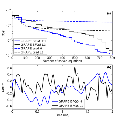
Figure 5: (Color online) (a) Cost function versus number of solved equations for conjugate gradient (grad) and BFGS optimization schemes, and for search directions obtained from Eqs. (6,7) with $H^{1}$ or $L^{2}$ norm, respectively. (b) Optimal control parameters $\lambda(t)$ for BFGS solutions.

Figure 5(a) shows the terminal cost function $J_{T}$ versus the number of solved equations of motion $n$ for the different GRAPE schemes. It is evident that the conjugate gradient solutions reach a plateau after a certain number of iterations. In contrast, the BFGS solutions decrease significantly even at later stages of the optimization. We attribute this behavior to the use of the second order derivative information. The GRAPE BFGS scheme, which estimates the Hessian of $J$ in addition to $\nabla_{\lambda}J$, can take larger steps to cross flat regions of $J$, contrary to the (first-order) GRAPE gradient scheme, which gets stuck.

Figure 5(b) shows the control fields for the GRAPE BFGS schemes. Although both optimization strategies perform equally well, the solutions obtained with $H^{1}$ norm are smoother and probably better suited for experimental implementation.

Figure 6: (Color online) Same as Fig. 5 but for Krotov optimization. We investigate the influence of different mixing parameters $k$ between the old and new control fields, see Eq. (10), as well as a scheme with an adaptive $k$ choice (see text for details). KBFGS reports the optimization result for a combination of Krotov’s method with BFGS Eitan et al. (2012).

Figure 6 presents (a) $J_{T}$ versus $n$ and (b) the control parameters for the Krotov optimization. The solid line with $k=0.005$ in panel (a) is identical to the one shown in Fig. 4. When we increase $k$ (black line) the cost function drops more rapidly. However, we found that larger $k$ values can lead to sharp variations in $\lambda(t)$ which might be problematic for experimental implementations, as will be discussed in more detail below.

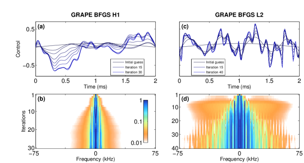
Figure 7: (Color online) (a,c) Evolution of control parameters during the optimization process for GRAPE. (b,d) Density plot of power spectra of the control parameters displayed in panels (a,c). We use a logarithmic color scale. In panels (b) and (d) the numbers of iterations are chosen such that the final cost function $J_{T}$ becomes approximately $10^{-2}$, the numbers of solved equations (see Figs. 2 and 4) are approximately (b) 500 and (d) 700.

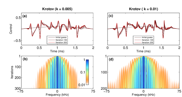
Figure 8: (Color online) Same as Fig. 7 but for Krotov optimization. The numbers of solved equations are (b) 600 and (d) 400.

In Fig. 6 we additionally display results for a simulation using a combination of Krotov’s method with the BFGS scheme (KBFGS) Eitan et al. (2012). The performance of KBFGS is similar to the simpler optimization procedure of Eq. (10), a finding in accordance with Ref. Eitan et al. (2012). We attribute this to the fact that within the Krotov scheme only a small portion of the control landscape is explored, because the monotonic convergence enforces small control updates, in contrast to GRAPE where larger regions are scanned by the line search. As consequence, the improvement in the Krotov search direction via the Hessian is minimal.

Finally, the dashed line for adaptive $k$ shows results for an optimization that starts with a small $k$ value, which subsequently increases in each iteration until the cost decreases by a desired amount (here 2.5 per cent) within one iteration. This $k$ value is then kept constant for the rest of the optimization. The idea behind this strategy is that the choice of $k$ is crucial for convergence, but the optimal value is different for each problem. Generally, finding a suitable value for $k$ requires some trial and error.

IV.4 Features of the Control

For many experimental implementations it is indispensable to use smooth control parameters. In the following we investigate the smoothness of the optimal controls obtained by the different optimization methods.

Figure 7(a) shows for GRAPE BFGS H1 the evolution of the $\lambda(t)$ values during optimization. One observes that during the first few iterations the characteristic features of $\lambda(t)$ emerge, which then become refined in the course of further iterations. Fig, 7(b) reports the power spectra (square moduli of Fourier transforms) of the $\lambda(t)$ history during optimization. During the first say 20 iterations the Fourier-transformed control parameter $\tilde{\lambda}(\nu)$ spectrally broadens, indicating the emergence of sharp features during optimization. With increasing iterations the spectral width of $\tilde{\lambda}(\nu)$ remains approximately constant.

Results of the GRAPE BFGS L2 optimization are shown in Figs. 7(c,d). We observe that, in contrast to the H1 results, $\lambda(t)$ acquires sharp features during optimization, as also reflected by the broad power spectrum. This is because initially the gradient $\nabla_{\lambda}J$, which determines the search direction for improved control parameters, exhibits strong variations. These variations are washed out in the H1 optimization through the solution of the Poisson equation, see Eq. (7), leading to significantly smoother control parameters.

In GRAPE, the user must additionally provide the weighting factor $\gamma$ of Eq. (3) that determines the relative importance of terminal cost and control smoothness. For the problems under study, we found that the performance of GRAPE does not depend sensitively on the value of $\gamma$, and we usually use a small value such that the cost is dominated by the terminal cost.

Figs. 8(a,c) show the $\lambda(t)$ history during a Krotov optimization for different step sizes $k$, and panels (b,d) report the corresponding power spectra. In comparison to the GRAPE BFGS H1 optimization, the power spectra are significantly broader, in particular for the larger $k$ values. This is due to the fact that in the functional used for the Krotov optimization there is no penalty term that enforces smoothness of the control (and thus a narrow spectrum).

The choice of the step size $k$ is rather critical for the Krotov performance. With increasing $k$ the cost function decreases more rapidly during optimization. However, values of $k$ that are too large can lead to numerical instabilities. These instabilities result from the discretization of the update equation; mathematically, Krotov is only guaranteed to converge monotonically for any value of $k$ if the control problem is continuous.

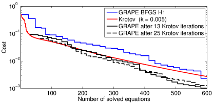
Figure 9: (Color online) Same as Fig. 4, but for a combined GRAPE–Krotov scheme where one initially starts with the Krotov method and switches to GRAPE after a given number of iterations.

One might wonder whether a combination of both approaches would give the best of two worlds. In Fig. 9 we present results for simulations where we start with a Krotov optimization and switch to GRAPE after a given number of iterations. As can be seen, the performance of this combined optimization does not offer a particular advantage over genuine GRAPE or Krotov optimizations. This is probably due to differences between the optimal control fields $\lambda(t)$ obtained by the two approaches, such that $\lambda(t)$ needs to be significantly modified when changing from one scheme to the other. In addition, the BFGS search algorithm of GRAPE uses the information of previous iterations in order to estimate the Hessian of the control space, and this information is missing when changing schemes.

V Conclusions and Outlook

Based on the two examples investigated in the previous section, namely wavefunction splitting and shaking in a magnetic microtrap, we now set out to analyze the advantages and disadvantages of the GRAPE and Krotov optimization methods which are tied to the functional that is minimized in each case.

First, when the optimization converges fast to an optimal solution, such as for wavefunction splitting investigated in Sec. IV.1, both optimization algorithms perform equally well, even without carefully tuning the free parameters $\gamma$ or $k$. For such problems, the choice of algorithm is a matter of personal preference. On the other hand, for optimization problems with slow convergence, such as wavefunction shaking, more care has to be taken. Specifically, there are significant differences between the two algorithms in terms of free parameters vs. speed of convergence as well as possible cost functionals vs. features of the obtained optimal control.

While GRAPE BFGS utilizes a line search to ensure monotonic convergence and to obtain the optimal step size in each iteration, the speed of convergence in Krotov’s method is mainly determined by the free parameter $k$. On the one hand this means that GRAPE BFGS works better “out of the box” since it automatically determines the best step size in each step. On the other hand, the convergence is slowed down due to the necessity of a line search.

It is also evident from our results that both algorithms yield controls with features that can be understood in terms of additional costs introduced in the functional. For GRAPE we use a cost that penalizes a large derivative of the control which results in smooth controls in the end. For Krotov’s method we employ a penalty on changes in the amplitude of the control in each iteration. Correspondingly this leads to controls that have a smaller integrated intensity and come at the cost of a less smooth control.

In principle it is conceivable to modify the Krotov algorithm to take into account an additional cost term on the derivative of the control. While we conjecture that this will lead to controls that are comparable with those obtained in the GRAPE framework, the necessary modification of the Krotov algorithm is beyond the scope of the current work.

In the context of controlling Bose-Einstein condensates with experimentally smooth controls, the optimization with the GRAPE BFGS method, a functional enforcing smoothness, and use of the $H^{1}$ norm appears to be the method of choice. It is a black–box scheme with practically no problem-dependent parameters, it gives the desired smooth control fields, and works for various nonlinearity parameters $\kappa$.

In contrast, the Krotov optimization without an appropriate penalty term in the functional can converge faster but usually also leads to sharp features in the control. A sensitive choice of the step size $k$ is indispensable to achieve a compromise between fast convergence and smoothness. If smoothness is not an issue or extremely fast convergence is needed, the Krotov method is preferable.

A combination of GRAPE and Krotov in the sense of switching from one method to the other during the optimization did not result in any significant gain. This is explained by the different control solutions that are found by the different methods which do not easily facilitate a transition between them. It points to the fact that many control solutions exist and which solution is identified by the optimization depends strongly on the additional constraints Palao et al. (2013) as well as the optimization method.

Appendix A

In this appendix we briefly show how to numerically solve the equation

$$\lambda^{(i+1)}(t)=\lambda^{(i)}(t)+S(t)\,\mathfrak{Re}\,\bigl{<}p^{(i)}(t)\bigr{|}\left[\frac{\partial V}{\partial\lambda}\Bigl{|}_{\lambda^{(i+1)}(t)}\right]\bigl{|}\psi^{(i+1)}(t)\bigr{>}\,,$$ (11)

which differs from Eq. (10) in that the potential derivative is evaluated for $\lambda^{(i+1)}(t)$. Things can be easily generalized for the additional $\sigma(t)$ term of Eq. (9). Let $\lambda_{0}(t)$ denote an initial guess for the solution of Eq. (11), e.g. the solution of Eq. (10). We now set $\lambda^{(i+1)}(t)=\lambda_{0}(t)+\delta\lambda(t)$, where $\delta\lambda(t)$ is assumed to be a small quantity. Thus, we can expand the second term on the right hand side of Eq. (11) in lowest order of $\delta\lambda(t)$ to obtain

$$\lambda_{0}(t)+\delta\lambda(t)\approx\lambda^{(i)}(t)+S(t)\,\mathfrak{Re}\,\bigl{<}p^{(i)}(t)\bigr{|}\left[\frac{\partial V}{\partial\lambda}\Bigl{|}_{\lambda_{0}(t)}+\frac{\partial^{2}V}{\partial\lambda^{2}}\Bigl{|}_{\lambda_{0}(t)}\delta\lambda(t)\right]\bigl{|}\psi^{(i+1)}(t)\bigr{>}\,.$$ (12)

Separating the contributions of $\delta\lambda$ from the rest, we get

$$\left(1-S(t)\,\mathfrak{Re}\,\bigl{<}p^{(i)}(t)\bigr{|}\left[\frac{\partial^{2}V}{\partial\lambda^{2}}\Bigl{|}_{\lambda_{0}(t)}\right]\bigl{|}\psi^{(i+1)}(t)\bigr{>}\right)\delta\lambda(t)\approx-(\lambda_{0}(t)-\lambda^{(i)}(t))+S(t)\bigl{<}p^{(i)}(t)\bigr{|}\left[\frac{\partial V}{\partial\lambda}\Bigl{|}_{\lambda_{0}(t)}\right]\bigl{|}\psi^{(i+1)}(t)\bigr{>}\,,$$ (13)

which can be solved for $\delta\lambda(t)$. If $|\delta\lambda(t)|<\varepsilon$ is smaller than some small tolerance $\varepsilon$, we set $\lambda^{(i+1)}(t)\to\lambda_{0}(t)+\delta\lambda(t)$. Otherwise we set $\lambda_{0}(t)\to\lambda_{0}(t)+\delta\lambda(t)$ and repeat the Newton iteration until convergence. Typically only few iterations are needed to reach tolerances of the order of $\varepsilon=10^{-6}$.

References

- Sayrin et al. (2011) C. Sayrin, I. Dotsenko, X. Zhou, B. Peaudecerf, T. Rybarczyk, S. Gleyzes, P. Rouchon, M. Mirrahimi, H. Amini, M. Brune, et al., Nature 477, 73–77 (2011).
- Bücker et al. (2011) R. Bücker, J. Grond, S. Manz, T. Berrada, T. Betz, C. Koller, U. Hohenester, T. Schumm, A. Perrin, and J. Schmiedmayer, Nature Phys. 7, 508 (2011).
- van Frank et al. (2014) S. van Frank, A. Negretti, T. Berrada, R. Bücker, S. Montangero, J. F. Schaff, T. Schumm, T. Calarco, and J. Schmiedmayer, Nature Commun. 5, 4009 (2014).
- Lapert et al. (2012) M. Lapert, Y. Zhang, M. A. Janich, S. J. Glaser, and D. Sugny, Sci. Rep. 2, 589 (2012).
- Häberle et al. (2013) T. Häberle, D. Schmid-Lorch, K. Karrai, F. Reinhard, and J. Wrachtrup, Phys. Rev. Lett. 111, 170801 (2013).
- Rybak et al. (2011) L. Rybak, S. Amaran, L. Levin, M. Tomza, R. Moszynski, R. Kosloff, C. P. Koch, and Z. Amitay, Phys. Rev. Lett. 107, 273001 (2011).
- González-Férez and Koch (2012) R. González-Férez and C. P. Koch, Phys. Rev. A 86, 063420 (2012).
- Rice and Zhao (2000) S. A. Rice and M. Zhao, Optical control of molecular dynamics (John Wiley & Sons, 2000).
- Brumer and Shapiro (2003) P. Brumer and M. Shapiro, Principles and Applications of the Quantum Control of Molecular Processes (Wiley Interscience, 2003).
- Tannor et al. (1992) D. Tannor, V. Kazakov, and V. Orlov, in Time-dependent quantum molecular dynamics, edited by J. Broeckhove and L. Lathouwers (Plenum, 1992), pp. 347–360.
- Werschnik and Gross (2007) J. Werschnik and E. K. U. Gross, J. Phys. B 40, R175 (2007).
- Palao and Kosloff (2002) J. P. Palao and R. Kosloff, Phys. Rev. Lett. 89, 188301 (2002).
- Doria et al. (2011) P. Doria, T. Calarco, and S. Montangero, Phys. Rev. Lett. 106, 190501 (2011).
- Kaiser and May (2004) A. Kaiser and V. May, J. Comp. Phys. 121, 2528 (2004).
- Caneva et al. (2011) T. Caneva, T. Calarco, and S. Montangero, Phys. Rev. A 84, 022326 (2011).
- Konnov and Krotov (1999) A. Konnov and V. Krotov, Automation and Remote Control 60, 1427 (1999).
- Sklarz and Tannor (2002) S. E. Sklarz and D. J. Tannor, Phys. Rev. A 66, 053619 (2002).
- Khaneja et al. (2005) N. Khaneja, T. Reiss, C. Kehlet, T. Schulte-Herbrüggen, and S. J. Glaser, J. Mar. Res. 172, 296 (2005).
- Machnes et al. (2011) S. Machnes, U. Sander, S. J. Glaser, P. de Fouquières, A. Gruslys, S. Schirmer, and T. Schulte-Herbrüggen, Phys. Rev. A 84, 022305 (2011).
- Eitan et al. (2012) R. Eitan, M. Mundt, and D. J. Tannor, Phys. Rev. A 83, 053426 (2012).
- Caneva et al. (2009) T. Caneva, M. Murphy, T. Calarco, R. Fazio, S. Montangero, V. Giovannetti, and G. E. Santoro, Phys. Rev. Lett. 103, 240501 (2009).
- Hohenester et al. (2007) U. Hohenester, P. K. Rekdal, A. Borzi, and J. Schmiedmayer, Phys. Rev. A 75, 023602 (2007).
- Hohenester (2014) U. Hohenester, Comp. Phys. Commun. 185, 194 (2014).
- Reich et al. (2012) D. M. Reich, M. Ndong, and C. P. Koch, J. Chem Phys. 136, 104103 (2012).
- Shin et al. (2004) Y. Shin, M. Saba, T. A. Pasquini, W. Ketterle, D. E. Pritchard, and A. E. Leanhardt, Phys. Rev. Lett. 92, 050405 (2004).
- Schumm et al. (2005) T. Schumm, S. Hofferberth, L. M. Andersson, S. Wildermuth, S. Groth, I. Bar-Joseph, J. Schmiedmayer, and P. Krüger, Nature Phys. 1, 57 (2005).
- Grond et al. (2010) J. Grond, U. Hohenester, I. Mazets, and J. Schmiedmayer, New J. Phys. 12, 065036 (2010).
- Peirce et al. (1988) A. P. Peirce, M. A. Dahleh, and H. Rabitz, Phys. Rev. A 37, 4950 (1988).
- Bücker et al. (2013) R. Bücker, T. Berrada, S. van Frank, T. Schumm, J. F. Schaff, J. Schmiedmayer, G. Jäger, J. Grond, and U. Hohenester, J. Phys. B 46, 104012 (2013).
- Leggett (2001) A. Leggett, Rev. Mod. Phys. 73, 307 (2001).
- Grond et al. (2009) J. Grond, G. von Winckel, J. Schmiedmayer, and U. Hohenester, Phys. Rev. A 80, 053625 (2009).
- Jäger and Hohenester (2013) G. Jäger and U. Hohenester, Phys. Rev. A 88, 035601 (2013).
- Borzi and Hohenester (2008) A. Borzi and U. Hohenester, SIAM Journal of Scientific Computing 30, 441 (2008).
- von Winckel and Borzi (2008) G. von Winckel and A. Borzi, Inverse Problems 24, 034007 (2008).
- Dion and Cances (2007) C. M. Dion and E. Cances, Comp. Phys. Commun. 177, 787 (2007).
- Bertsekas (1999) D. P. Bertsekas, Nonlinear Programming (Athena Scientific, Cambridge, UK, 1999).
- Palao and Kosloff (2003) J. P. Palao and R. Kosloff, Phys. Rev. A 68, 062308 (2003).
- Lesanovsky et al. (2006) I. Lesanovsky, T. Schumm, S. Hofferberth, L. M. Andersson, P. Krüger, and J. Schmiedmayer, Phys. Rev. A 73, 033619 (2006).
- Palao et al. (2013) J. P. Palao, D. M. Reich, and C. P. Koch, Phys. Rev. A 88, 053409 (2013).