Weak Values and Modular Variables From a Quantum Phase Space Perspective

Abstract

We address two major conceptual developments introduced by Aharonov and collaborators through a quantum phase space approach: the concept of modular variables devised to explain the phenomena of quantum dynamical non-locality and the two-state formalism for Quantum Mechanics which is a retrocausal time-symmetric interpretation of quantum physics which led to the discovery of weak values. We propose that a quantum phase space structure underlies these profound physical insights in a unifying manner. For this, we briefly review the Weyl-Wigner and the coherent state formalisms as well as the inherent symplectic structures of quantum projective spaces in order to gain a deeper understanding of the weak value concept.

We also review Schwinger’s finite quantum kinematics so that we may apply this discrete formalism to understand Aharonov’s modular variable concept in a different manner that has been proposed before in the literature. We discuss why we believe that this is indeed the correct kinematic framework for the modular variable concept and how this may shine some light on the physical distinction between quantum dynamical non-locality and the kinematic non-locality, generally associated with entangled quantum systems.

1 Introduction

There are two major conceptual developments introduced by Aharonov and collaborators which we believe provide the underpinnings for a more fundamental understanding of Quantum Mechanics (QM). The first is the concept of modular variables which was devised to characterize the kind of dynamical non-locality that become widely recognized when he, together with David Bohm, shocked the world of physics in the late fifties with the introduction of the so called Aharonov-Bohm (AB) effect aharonov_bohm1959 . Their paper discussed a situation where the wave functions that represent the electrons suffer a phase shift from the magnetic field of a solenoid even without having had any direct contact with the field. In aharonovpendletonpetersen , Aharonov, Pendleton and Petersen introduced the concept of modular variables to explain this kind of non-local quantum effect as the modular momentum exchange between particles and fields. This is contrary to the usual view where the AB phenomenon is explained by a local interaction between the particles and field potentials, even if the potentials are considered somewhat unphysical because they are defined only up to some gauge transformation. Even the interference effects of a single particle passing through a slit must be described by the this non-local dynamical effect. Imagine a particle beam diffracting through a two-slit apparatus (with a distance $L$ between the slits). The Schrödinger wave-like picture is capable of explaining the interference by analogy with classical wave-like interferometry. But this picture is misleading and it is not capable of giving a full quantum mechanical explanation of the underlying phenomena. One can lower the intensity of the beam until only one single particle arrives at the apparatus at each moment. One may choose to open or close one of the slits until the last instant. How does one of the slits “know” about the other one instantaneously? To answer this question, one can devise the following simplified mathematical model: Consider the problem as a two-dimensional setting in the $x$-$y$ plane with the beam in the positive $y$ direction and the apparatus with the slits in the $x$ direction. We consider only the $x$ direction where the particle “feels” a potential $\phi(x)$. It is not difficult to see that the translation operator $\hat{V}_{L}=e^{i\hat{P}L}$ obeys a non-local equation of motion in the Heisenberg picture:

$$\frac{d}{dt}\left(\hat{V}_{L}\right)=i\left[\phi(\hat{Q}),\hat{V}_{L}\right]=i\left(\phi(\hat{Q})-\phi(\hat{Q}+L)\right)\hat{V}_{L}$$ (1)

This kind of dynamical non-locality seems to be of a fundamentally different physical nature from that of the kinematic type of non-locality that occurs for entangled systems that are spatially appart as for instance, the paradigmatic EPR pair of particles. One of the main results of this paper is to advance our understanding of the differences between these two types of non-locality by using Schwinger´s finite kinematic formalism in order to present an alternative approach for the construction of the Hilbert spaces for modular variables. Though the AB effect is nowadays discussed in any undergraduate text-book of QM, according to Aharonov, the true reason for these strange phenomena, where electric and magnetic fields seem to be capable of exerting “action at a distance” upon charged quantum particles, has not been generally appreciated. Aharonov developed an intuition on this concept through the Heisenberg picture of QM and he has argued in a convincing manner that it is easier to think of this quite subtle issue through Heisenberg’s picture rather than Schrödinger’s wave-like picture aharonov2003book . In fact, in the early seventies, Heisenberg himself was very pleased to learn from Aharonov how to describe the concept of quantum interference based on his own formulation of quantum physics instead of the usual particle-wave (Schrödinger-like) approach aharonov2013 .

The second concept is the advancement of the two-state formalism for QM AharonovBergmannLebowitz . This is a radically different (time-symmetric) view of QM that has also been developed since the sixties and implies a notion of retrocausality in quantum physics which led to the discovery of weak values AharonovAlbertVaidman . The development of the concept of weak values and weak measurements has spanned a number of important theoretical and experimental breakthroughs from quantum counterfactual investigations to high precision metrology and even led to some purely mathematical ideas such as the concept of superoscillations aharonov2002revisiting ; dixon2009 ; hosten2008 ; berry2010typical .

We recall that new points of view concerning a certain subject are always welcome. It is common historical knowledge that the establishment of bridges between distinct disciplines is usually a very fruitful enterprise for both subjects. This interplay has brought us (from at least Newton and Galileo to Einstein and Minkowski, passing through Euler, Lagrange, Hamilton, Maxwell and many others) a wonderful multitude of results where mathematical structures are discovered by contemplating natures wonders and physical theories are guessed from deep and beautiful mathematics. In this paper, we approach the many deep physical insights of Aharonov with an eye towards the quantum phase space structure which we propose may underlie them in a unifying  manner.

The structure of this paper is as follows: in section 2, we review the mathematical structure of classical phase space as the geometric notion that “classical mechanics is symplectic geometry” arnold ; abraham ; sudarshan2006 so that the focus is the natural symplectic structure of cotangent bundles of configuration manifolds of classical particles restricted to holonomic constraints. This symplectic geometric structure appears consistently in almost all the topics covered in this paper. In section 3, we present an intrinsic formulation for the operator algebra of the WW Transform (similar to Dirac’s Bra and Ket notation) that is necessary to construct this formalism in a more compact and elegant way than the usual manner. In section 4, we discuss the natural symplectic structure that projective spaces of finite dimensional Hilbert spaces inherit from their Hermitian structure and for this reason are somewhat structurally analogous to classical phase spaces. In section 5, we briefly review the coherent state concept in terms of the WW basis mainly to set the stage for a discussion of the quantum transforms that implement linear area preserving maps on the phase plane. In section 6, we apply some of these ideas to a phase space study of the weak value concept, which has become an important theoretical and experimental tool in modern investigations of quantum physics. We look at the phase space of the measuring apparatus that performs the weak value measurement of some quantum system. In section 7, we approach the weak measurements and von Neumann pre-measurements by the opposite approach: in particular, we look instead to the geometric structure of the measured system. In section 8, we review the geometry of deterministic measurements and of completely uncertain operators. We also discuss some examples that can be seen as partially deterministic operators. This is the starting point in order to one fully appreciate the Heisenberg picture approach that Aharonov has championed for the description of quantum interference phenomena. Finally, in section 9, we introduce the modular variable concept. We review the original approach due to Aharonov and collaborators for the construction of an explicit Hilbert space (an appropriate “qudit space” for modular variables). We then review Schwinger’s finite quantum kinematics in order to apply this discrete formalism to understand Aharonov’s modular variable concept in a different manner that has been proposed until now in the literature. In the original approach, the total quantum space can be thought as the direct orthogonal sum between the modular variable qudit space and “the rest” of the infinite dimensional quantum space. Within the Schwinger formalism, we introduce a new proposal based on the tensor product between the modular variable qudit space and the rest of the quantum space. While there are some number-theoretic subtleties in order to perform this construction, we discuss some of the advantages of considering this Schwinger finite quantum kinematic-based proposal as the correct “kinematic arena” for the modular variable concept. In section 10 we finalize with some concluding remarks and we also set stage for further research.

2 The Mathematical Structure of Classical Phase Space

(The main references for this section are arnold and abraham )

What is meant here by a “classical structure” is the totality of the mathematical formalism associated with conservative (Hamiltonian) dynamical systems, i.e.:

1. An even-dimensional differential manifold $M$
   $(\dim M=2n)$;

2. A canonical coordinate system $(q^{i},p_{i})$
   $(i=1,2,\ldots,n)$ over $M$, where $n$ is the number of degrees of freedom of the system;

3. A non-degenerate closed 2-form $\Omega$ on $M$.

In other words: $d\Omega=0$ and the non-degeneracy meaning that: $\Omega(V,W)=0\Rightarrow V=0$ or $W=0$, $\forall\text{ }V,W\in T_{p}M$ and $\forall\text{ }p\in M$ and where $TM$ is the tangent bundle of $M$ and $T_{p}M$ is the tangent space (fiber) of $M$ at $p\in M$. A differential manifold with the above structure is called symplectic. A theorem due to Darboux guarantees that given a point $p\in M$, there is always an open set of $M$ that contains $p$ and that admits a pair of canonical coordinates ($q^{i},p_{i}$ ) such that $\Omega=-dp_{i}\wedge dq^{i}$ (we use henceforth the sum convention unless we explicitly state the contrary). In Classical Newtonian Mechanics, the above structure arises naturally as the cotangent bundle of a configuration manifold $Q$ (of dimension $n$) of $m$ particles submitted to $3m-n$ holonomic constraints: $M=T^{\ast}Q$. In fact, any cotangent bundle has a natural 1-form $\theta=p_{i}dq^{i}$, where $q^{i}$ are the coordinates of $Q$ and $p^{i}$ are the coordinates of the co-vectors of $T^{\ast}Q$. It is easy to verify that indeed the 2-form defined by $\Omega=-d\theta$ satisfies automatically the conditions (1-3). Yet not all symplectic manifolds are cotangent bundles.

An example that will be of great importance for us later is that of quantum projective spaces. We may define a dynamical structure on a symplectic manifold (the phase space) by introducing a real-value Hamiltonian function $H:M\rightarrow\mathbb{R}$ which maps each point in $M$ to a definite energy value. We can also define a symplectic gradient $X_{H}$ of $H$ (through $\Omega$) by the following relation $\Omega(X_{H},Y)=dH(Y)$ for any vector field $Y$ defined over $M$. In canonical coordinates, the vector field $X_{H}$ is given by

$$X_{H}=\frac{\partial H}{\partial p_{i}}\frac{\partial}{\partial q^{i}}-\frac{\partial H}{\partial q^{i}}\frac{\partial}{\partial p_{i}}$$ (2)

The motion of the system is given by the integral curves of $X_{H}$ and the first order ODE’s associated to them are the well-known Hamilton equations:

$$\dot{q}^{i}=\frac{\partial H}{\partial p_{i}}\qquad\text{and}\qquad\dot{p}_{i}=-\frac{\partial H}{\partial q^{i}}$$ (3)

A classical observable is any well-behaved real function defined on $M$. For example, the observables $Q^{i}$ and $P_{i}$ are respectively the $i$-th components of the generalized position and momentum

$$\begin{array}[]{c}Q^{i}:M\rightarrow\mathbb{R}\\ (q^{i},p_{i})\longrightarrow q^{i}\end{array}\qquad\text{and}\qquad\begin{array}[]{c}P_{i}:M\rightarrow\mathbb{R}\\ (q^{i},p_{i})\longrightarrow p_{i}\end{array}$$

The Poisson brackets of two arbitrary observables $f$ and $g$ can then be defined as:

$$\{f,g\}=\Omega(X_{f},X_{g})=\frac{\partial g}{\partial p_{i}}\frac{\partial f}{\partial q^{i}}-\frac{\partial f}{\partial p_{i}}\frac{\partial g}{\partial q^{i}},$$ (4)

and the temporal evolution of a general observable
$O(q^{i},p_{i})$ can be written as

$$\frac{dO}{dt}=\{O,H\}$$ (5)

The different formulations of Quantum Mechanics have shown from the very beginning a close relation with the structure of classical analytical mechanics as one can infer from common denominations of quantum physics as like, for example, the “Hamiltonian operator” for the generator of time displacements and the formal analogies of equations like the Heisenberg equation and its classical analog given by (5) (we use henceforth $\hbar=1$ units)

$$i\frac{d\hat{O}}{dt}=[\hat{O},\hat{H}]$$ (6)

for the evolution of a quantum observable $\hat{O}$ and a classical observable $O\left(q^{i},p_{i}\right)$. Since then, some different formalisms that relate both structures have been introduced with a number of applications in physics. In the next sections, we review some of these formalisms such as the Weyl-Wigner transform theory and coherent state theory. In the final sections we show how these structures are intimately related to the concepts of weak values and modular variables.

One of the most fundamental differences between quantum physics and classical physics is that the first admits the possibilities of both discrete and continuous observables while the second admits only continuous quantities. In the next section we will discuss only continuous phase spaces and in the following sections we will address “finite” or “discrete” phase spaces when we introduce the Schwinger formalism as a tool towards a deeper understanding of the concept of modular variables.

3 The Weyl-Wigner Formalism

(The main references for this section are degroot and sakurai )

3.1 The Fourier Transform Operator

Consider a quantum system defined by the motion of a single non-relativistic particle in one dimension. Let $\left\{\left|q(x)\right\rangle\right\}$ and $\left\{\left|p(x)\right\rangle\right\}$ $(-\infty<x<\infty)$ represent respectively the quantum eigenkets of the position and momentum observables. In other words, we have:

$$\hat{Q}\left|q(x)\right\rangle=x\left|q(x)\right\rangle\qquad\text{and}\qquad\hat{P}\left|p(x)\right\rangle=x\left|p(x)\right\rangle$$ (7)

where $\hat{Q}$ and $\hat{P}$ are the position and momentum operators, respectively. It is important to notice here that we use a slightly different notation than the usual choice. For instance, the ket $\left|q(x)\right\rangle$ is an eigenvector of $\hat{Q}$ with eigenvalue $x$. That is, we distinguish the “kind” of eigenvector (position or momentum) from its eigenvalue. This is different from the more common notation where $\left|q\right\rangle$ and $\left|p\right\rangle$ represent both the type of eigenket (respectively position and momentum in this case) and also the eigenvalue in the sense that $\hat{Q}\left|q\right\rangle=q\left|q\right\rangle$ and $\hat{P}\left|p\right\rangle=p\left|p\right\rangle$. As we shall see shortly, our choice of notation will allow us to write some equations in a more compact and elegant form. We shall designate the vector space generated by these basis as $W^{(\infty)}$. This is clearly not a Hilbert space since $W^{(\infty)}$ accommodates “generalized vectors” as $\left|q(x)\right\rangle$ and $\left|p(x)\right\rangle$ that have “infinite norm”. A rigorous foundation for this construction can be given within the so called rigged vector space formalism (see arnobohm for more details on this issue). Later on, we will present a natural construction of these spaces as a continuous heuristic limit of analogous well-defined finite dimensional spaces originally due to Schwinger.

Let $\hat{V}_{\xi}$ and $\hat{U}_{\eta}$ $(-\infty<\xi,\eta<\infty)$ be a pair of unitary operators that implement the one parameter abelian group of translations on respectively the position and momentum basis in the sense that

$$\hat{V}_{\xi}\left|q(x)\right\rangle=\left|q(x-\xi)\right\rangle\quad\text{and}\quad\hat{U}_{\eta}\left|p(x)\right\rangle=\left|p(x+\eta)\right\rangle$$ (8)

The hermitian generators of $\hat{V}_{\xi}$ and $\hat{U}_{\eta}$ are the momentum and position observables, respectively:

$$\hat{V}_{\xi}=e^{i\xi\hat{P}}\qquad\text{and}\qquad\hat{U}_{\eta}=e^{i\eta\hat{Q}}$$ (9)

so that

$$\hat{V}_{\xi}\left|p(x)\right\rangle=e^{i\xi x}\left|p(x)\right\rangle\quad\text{and}\quad\hat{U}_{\eta}\left|q(x)\right\rangle=e^{i\eta x}\left|q(x)\right\rangle$$ (10)

The translation operators also obey the so called Weyl relation:

$$\hat{V}_{\xi}\hat{U}_{\eta}=\hat{U}_{\eta}\hat{V}_{\xi}e^{i\eta\xi}$$ (11)

which can be thought as an exponentiated version of the familiar Heisenberg relation:

$$[\hat{Q},\hat{P}]=i\hat{I}$$ (12)

The basis $\left|q(x)\right\rangle$ and $\left|p(x)\right\rangle$ are both complete and normalized in the sense that

$$\hat{I}=\int_{-\infty}^{+\infty}dx\left|q(x)\right\rangle\left\langle q(x)\right|=\int_{-\infty}^{+\infty}dx\left|p(x)\right\rangle\left\langle p(x)\right|$$ (13)

and

$$\left\langle q(x)\right|q(x\prime)\rangle=\left\langle p(x)\right|p(x\prime)\rangle=\delta(x-x\prime)$$ (14)

The overlap between the position and momentum eigenstate is given by the well-known plane wave function:

$$\left\langle q(x)\right|p(x\prime)\rangle=\frac{1}{\sqrt{2\pi}}e^{ixx\prime}$$ (15)

Any arbitrary abstract state $\left|\psi\right\rangle$ has a “position basis wave function”given by $\left\langle q(x)\right|\psi\rangle$ and a “momentum basis wave function” given by $\left\langle p(x)\right|\psi\rangle$. The relation between both is given by the Fourier transform operator which is a unitary operator that takes one basis to another as

$$\hat{F}\left|q(x)\right\rangle=\left|p(x)\right\rangle$$ (16)

This operator can be defined in a more elegant and compact manner as:

$$\hat{F}=\int_{-\infty}^{+\infty}dx\left|p(x)\right\rangle\left\langle q(x)\right|$$ (17)

Note that the above equation could not have been written in such way within the conventional notation. We also have that

$$\hat{F}^{{\dagger}}\left|p(x)\right\rangle=\left|q(x)\right\rangle$$

and that $\hat{F}$ is unitary, which means that

$$\hat{F}^{{\dagger}}\hat{F}=\hat{I}$$

The Fourier transform of $\psi(x)=\left\langle q(x)\right|\psi\rangle$ is then $\left\langle q(x)\right|\hat{F}^{{\dagger}}\left|\psi\right\rangle=\left\langle p(x)\right|\psi\rangle=\tilde{\psi}(x)$, where we introduced here the tilde psi-function $\tilde{\psi}(x)$ as the Fourier transform of $\psi(x)$. The effect of the inverse transform Fourier operator over the position basis is given by

$$\hat{F}^{{\dagger}}\left|q(x)\right\rangle=\int_{-\infty}^{+\infty}dx\prime\left|q(x\prime)\right\rangle\left\langle p(x\prime)\right|q(x)\rangle$$

From the symmetries of (15) it is easy to see that $\left\langle p(x\prime)\right|q(x)\rangle=\left\langle q(x\prime)\right|p(-x)\rangle$ so that:

$$\hat{F}^{{\dagger}}|q(x)\rangle=\int_{-\infty}^{+\infty}dx\prime\left|q(x\prime)\right\rangle\left\langle q(x\prime)\right|p(-x)\rangle=\left|p(-x)\right\rangle$$

Analogously, we may write

$$\hat{F}^{2}\left|q(x)\right\rangle = \hat{F}\left|p(x)\right\rangle=\int_{-\infty}^{+\infty}dx\prime\left|p(x\prime)\right\rangle\left\langle q(x\prime)\right|p(x)\rangle$$

$$= \int_{-\infty}^{+\infty}dx\prime\left|p(x\prime)\right\rangle\left\langle p(x\prime)\right|q(-x)\rangle=\left|q(-x)\right\rangle$$

This implies that $\hat{F}^{2}$ is nothing else but the space inversion operator in $W^{(\infty)}$. Analogously one can deduce in a similar manner that

$$\hat{F}^{2}\left|p(x)\right\rangle=\left|p(-x)\right\rangle$$

This also implies that

$$\hat{F}^{4}=\hat{I}$$

which means that the spectrum of the Fourier operator $\hat{F}$ is constituted by the fourth roots of unity. We shall return to this issue in a later section. In a similar manner it is not difficult to show that

$$\hat{F}^{{\dagger}}\hat{U}_{\xi}\hat{F}=\hat{V}_{\xi}^{{\dagger}}\qquad\text{and}\qquad\hat{F}^{{\dagger}}\hat{V}_{\xi}\hat{F}=\hat{U}_{\xi}$$ (18)

and

$$\hat{F}\hat{V}_{\xi}\hat{F}^{{\dagger}}=\hat{U}_{\xi}^{{\dagger}}\qquad\text{and}\qquad\hat{F}\hat{U}_{\xi}\hat{F}^{{\dagger}}=\hat{V}_{\xi}$$ (19)

which implies the following two very important relations

$$\hat{F}^{2}\hat{U}_{\xi}\hat{F}^{2}=\hat{U}_{\xi}^{{\dagger}}\qquad\text{and}\qquad\hat{F}^{2}\hat{V}_{\xi}\hat{F}^{2}=\hat{V}_{\xi}^{{\dagger}}$$ (20)

3.2 An Intrinsic Formulation for the Weyl-Wigner Operator and Transform

We shall designate the space of linear operators over $W^{(\infty)}$ as $T_{1}^{1}(W^{(\infty)})$ and denote the “vectors”(the elements) $\hat{A},\hat{B},\hat{C}$,… of $T_{1}^{1}(W^{(\infty)})$ respectively by $|\hat{A})$,
$|\hat{B})$,$|\hat{C})$,…Following Schwinger schwinger , we introduce the well-known hermitian inner product, also known as the Hilbert-Schmidt inner product, in $T_{1}^{1}(W^{(\infty)})$ given by:

$$(\hat{A}|\hat{B})=tr(\hat{A}^{{\dagger}}\hat{B})$$ (21)

The space $T_{1}^{1}(W^{(\infty)})$ has an additional algebraic structure which turns it into an operator algebra. In fact, we have the following product $|\hat{A}).|\hat{B})=|\hat{A}.\hat{B})$, where $\hat{A}.\hat{B}$ is the usual operator product between $|\hat{A})$ and $|\hat{B})$. In this way we may identify the elements of $T_{1}^{1}(W^{(\infty)})$ with the elements of $T_{1}^{1}(T_{1}^{1}(W^{(\infty)}))$ in an unique manner through the obvious inclusion map

$$i:T_{1}^{1}(W^{(\infty)}) \rightarrow T_{1}^{1}(T_{1}^{1}(W^{(\infty)}))$$

$$\hat{A}\equiv|\hat{A}) \mapsto\breve{A},$$

such that $\breve{A}|\hat{B})=|\hat{A}.\hat{B})$. We will usually allow ourselves a slight abuse of language by dismissing any explicit mention to this inclusion map. For instance, consider the following identifications of the Identity Operator: $\hat{I}\equiv|\hat{I})\overset{i}{\equiv}\breve{I}$ . In this way one may define a set of operators $\hat{X}(\alpha)\equiv|\hat{X}(\alpha))$ to be complete in $T_{1}^{1}(W^{(\infty)})$, where $\alpha$ is a variable that takes values in some appropriate “index set”, if

$$\int d\alpha|\hat{X}(\alpha))(\hat{X}(\alpha)|=\breve{I}\equiv\hat{I}\equiv|\hat{I}),$$ (22)

where $d\alpha$ is an appropriate measure in the index set. Orthonormality can be written as

$$(\hat{X}(\alpha)|\hat{X}(\beta))=tr(\hat{X}^{{\dagger}}(\alpha)\hat{X}(\beta))=\delta(\alpha-\beta)$$ (23)

As an example, consider $|q(x)\rangle\langle p(y)|\equiv|x,y)$ with $x,y\in\mathbb{R}^{2}$. This set of $\mathbb{R}^{2}$-valued operators is indeed orthonormal in the sense that

$$(x,y|x\prime,y\prime)=\delta(x-x\prime)\delta(y-y\prime)$$ (24)

It is not difficult to prove that $(x,y|\hat{A})=\langle q(x)|\hat{A}|p(y)\rangle$ and $\int\int dxdy|x,y)(x,y|=\breve{I}$. These results can be used to prove another very convenient completeness relation for a set $\{\hat{X}(\alpha)\}$ as

$$\int d\alpha\hat{X}^{{\dagger}}(\alpha)\hat{A}\hat{X}(\alpha)=(tr\hat{A})\hat{I},\quad\forall\text{ }\hat{A}\in T_{1}^{1}(W^{(\infty)})$$

We can now define a set of operators (the so called Weyl-Wigner operators) also parameterized by the phase space plane $(x,y)\in\mathbb{R}^{2}$ in the following intrinsic manner

$$\hat{\Delta}(x,y)=2\hat{V}_{y}^{{\dagger}}\hat{U}_{2x}\hat{V}_{y}^{{\dagger}}\hat{F}^{2}$$ (25)

With aid of (20), one can easily prove the following important properties:

• hermiticity:

  $$\hat{\Delta}^{{\dagger}}(x,y)=\hat{\Delta}(x,y)$$ (26)

• unit trace:

  $$tr(\hat{\Delta}(x,y))=(\hat{\Delta}(x,y)|\hat{I})=1$$ (27)

• orthonormality of ${\frac{1}{\sqrt{2\pi}}\hat{\Delta}(x,y)}$:

  $$(\hat{\Delta}(x,y)|\hat{\Delta}(x\prime,y\prime))=2\pi\delta(x-x\prime)\delta(y-y\prime)$$ (28)

• 1st form for the completeness of $\frac{1}{\sqrt{2\pi}}\hat{\Delta}(x,y)$:

  $$\frac{1}{2\pi}\int\int dxdy|\hat{\Delta}(x,y))(\hat{\Delta}(x,y)|=\hat{I}$$ (29)

• 2nd form of the completeness of $\frac{1}{\sqrt{2\pi}}\hat{\Delta}(x,y)$:

  $$\frac{1}{2\pi}\int\int dxdy\hat{\Delta}(x,y)\hat{A}\hat{\Delta}(x,y)=(tr\hat{A})\hat{I},\quad\forall\hat{A}$$ (30)

Some other properties (not so well-known) for the Weyl-Wigner operators are the following:

$$\hat{\Delta}^{2}(x,y)=4\hat{I}$$ (31)

$$\hat{F}^{2}\hat{\Delta}(x,y)\hat{F}^{2}=\hat{\Delta}(-x,-y)$$ (32)

$$\hat{\Delta}(0,0)=2\hat{F}^{2}$$ (33)

At this point, one can define the Weyl-Wigner Transform of an arbitrary Operator as

$$W\{\hat{A}\}(x,y)=(\hat{\Delta}(x,y)|\hat{A})=a(x,y)$$ (34)

The transform of $\hat{A}$ is in general a complex function $a(x,y)$ of the phase plane, but if $\hat{A}$ is hermitian, then $a(x,y)$ is clearly real-valued. One is tempted to see this transform as a map between quantum observables to “classical observables” in some sense. In fact, as we shall soon see, there is a certain sense where in the $\hbar\rightarrow 0$ limit, one can see that $a(x,y)$ goes indeed to the expected classical observable. Wigner introduced this transform to map density operators of mixed states to classical probability densities over phase space, but the fact is that these densities obey all axioms for a true probability distribution on phase space with the exception of positivity. In this way, the negativity of the transform of a density operator signals for a departure of classicality of the mixed state or some kind of measure of “quanticity” of the state.

3.3 The Classical Limit

The inner product between two operators $\hat{A}$ and $\hat{B}$ can be written in terms of their WW transforms as

$$(\hat{A}|\hat{B})=\frac{1}{2\pi}\int dxdy\overline{a}(x,y)b(x,y),$$ (35)

where $\overline{a}(x,y)$ is the c.c. of $a(x,y)$. The transform of a product of two arbitrary operators can be seen, after a tedious calculation, as

$$(\hat{\Delta}(x,y)|\hat{A}\hat{B})=a(x,y)\exp\Big{[}-\frac{i}{2}(\frac{\overleftarrow{\partial}}{\partial x}\frac{\overrightarrow{\partial}}{\partial y}-\frac{\overleftarrow{\partial}}{\partial y}\frac{\overrightarrow{\partial}}{\partial x})\Big{]}b(x,y),$$ (36)

where the arrows above the partial derivative operators indicate “which function” it operates on. With this result, it is not difficult to guess the very suggestive form of the WW transform of the commutator of two operators and (we momentarily restore $\hbar$ here explicitly) the following fact that the “classical limit” can be understood as

$$-2i\underset{\hbar\rightarrow 0}{\lim}\Big{(}\frac{1}{\hbar}(\hat{\Delta}(x,y)|[\hat{A},\hat{B}])\Big{)}$$

$$=2\underset{\hbar\rightarrow 0}{\lim}\Big{(}\frac{1}{\hbar}a(x,y)\sin\Big{[}\frac{\hbar}{2}\Big{(}\frac{\overleftarrow{\partial}}{\partial x}\frac{\overrightarrow{\partial}}{\partial y}-\frac{\overleftarrow{\partial}}{\partial y}\frac{\overrightarrow{\partial}}{\partial x}\Big{)}\Big{]}b(x,y)\Big{)}$$

$$=\{a(x,y),b(x,y)\}$$ (37)

One recognizes the last term of the above equation as the Poisson bracket of the classical observables $a(x,y)$ and $b(x,y)$. The operation defined by (36) establishes a non-commutative algebra over the real functions defined on phase space. It is also known as the star-product and it forms the basis of the non-commutative geometric point of view for quantization.

3.4 The Issue of the Number of Degrees of Freedom

The extension of the continuous WW formalism to two or more degrees of freedom is straightforward: For instance, let $|q(x)\rangle$ and $|q(y)\rangle$ be complete position eigenbasis for the $x$ and $y$ directions, respectively. Then, a point $\vec{r}$ of the plane is clearly represented by the tensor product state $|q(\vec{r})\rangle=|q(x)\rangle\otimes|q(y)\rangle$. The 2D translation operator

$$\hat{V}_{\vec{\xi}}=e^{i\vec{P}.\vec{\xi}}=e^{i\hat{P}_{x}\xi_{x}}\otimes e^{i\hat{P}_{y}\xi_{y}}$$ (38)

acts upon the $|q(\vec{r})\rangle$ basis by the expected manner as $\hat{V}_{\vec{\xi}}|q(\vec{r})\rangle=|q(\vec{r}-\vec{\xi})\rangle$. This can be clearly carried out for any number of degrees of freedom in the same way. For finite dimensional quantum spaces, things are not as simple as we shall see further ahead.

4 The Geometry of Quantum Mechanics

(The main references for this section are arnold , page and anandan1990 )

4.1 The Projective Space $\mathbb{CP}(N)$

Let us consider the $(N+1)$-dimensional quantum space $W^{(N+1)}$. This is a complex vector space together with an anti-linear map between $W^{(N+1)}$ and its dual $\overline{W}^{(N+1)}$:

$$\langle\text{ }\rangle:W^{(N+1)} \rightarrow\overline{W}^{(N+1)}$$

$$|\psi\rangle \mapsto\langle\psi|=(|\psi\rangle)^{{\dagger}}$$

that takes each ket state to its associated bra state through the familiar “dagger” operation. The inner product between $|\psi_{1}\rangle$ and $|\psi_{2}\rangle$ can then be defined as the natural action of $\langle\psi_{1}|$ over $|\psi_{2}\rangle$ in the usual Dirac notation $\left\langle\psi_{1}\right|\psi_{2}\rangle$. Following arnold , one can define Euclidean and symplectic metric structures on $W^{(N+1)}$ through the relations

$$G\left(|\psi_{1}\rangle,|\psi_{2}\rangle\right)=\operatorname{Re}\left\langle\psi_{1}\right|\psi_{2}\rangle\quad\text{and}\quad$$

$$\Omega\left(|\psi_{1}\rangle,|\psi_{2}\rangle\right)=\operatorname{Im}\left\langle\psi_{1}\right|\psi_{2}\rangle$$ (39)

From fundamental postulates of Quantum Mechanics, it is clear that a state vector $|\psi\rangle\in W^{(N+1)}$ is physically indistinguishable from the state vector $\lambda|\psi\rangle$ (for arbitrary $\lambda\in\mathbb{C}$). Thus, the true physical space of states of the theory is the so called “space of rays” or the complex projective space $\mathbb{CP}(N)$ defined by the quotient of $W^{(N+1)}$ by the above physically motivated equivalence relation.

Given an orthonormal basis $\{|u_{\sigma}\rangle\}$ $\sigma=0,1,2$,…, then a general state vector can be expanded as $|\psi\rangle=|u_{\sigma}\rangle z^{\sigma}$. One can map this state to a sphere $S^{2N+1}$ with squared radius given by $r^{2}=\bar{z}_{\sigma}z^{\sigma}$. We introduce projective coordinates

$$\xi^{i}=z^{i}/z^{0}$$ (40)

on $\mathbb{CP}(N)$ so that

$$z^{0}=re^{i\phi}/(1+\bar{\xi}_{j}\xi^{j})^{1/2}\qquad\text{with}\qquad i=1,\ldots,n,$$ (41)

where $\phi$ is an arbitrary phase factor. The Euclidean metric in $W^{(N+1)}$ (seen here as a $(2n+2)$-dimensional real vector space) can be written as

$$dl^{2}\left(W^{(N+1)}\right)=d\bar{z}_{\sigma}dz^{\sigma}=dr^{2}+dS^{2}(S^{2N+1})$$ (42)

where

$$dS^{2}(S^{2N+1})=(d\phi-A)^{2}+ds^{2}(\mathbb{CP}(N))$$

is the squared distance element over the space of normalized vectors and the one-form

$$A=\frac{i}{2}\frac{(\bar{\xi}_{i}d\xi^{i}-d\bar{\xi}_{i}\xi^{i})}{(1+\bar{\xi}_{i}\xi^{i})}$$

is the well known abelian connection of the $U(1)$ bundle over $\mathbb{CP}(N)$ page . The metric $ds^{2}(\mathbb{CP}(N))$ over the space of rays in projective coordinates is given explicitly by:

$$ds^{2}(\mathbb{CP}(N))=\frac{i}{2}\frac{[(1+\bar{\xi}_{i}\xi^{i})\delta_{k}^{j}-\bar{\xi}_{k}\xi^{j})]}{(1+\bar{\xi}_{i}\xi^{i})^{2}}d\bar{\xi}_{j}d\xi^{k}$$

and $\Omega=dA$ is a 2-form defined over $\mathbb{CP}(N)$ which makes it a symplectic manifold. These quantum symplectic spaces are physically very different in origin from their Newtonian counterparts.

The Newtonian phase spaces are cotangent bundles over some configuration manifold and as such they are always non-compact manifolds, while projective spaces are compact for finite $N$. For instance, $\mathbb{CP}(1)$ can be identified with a 2-sphere. The quantum projective spaces also have an additional structure given by their Riemannian metric, which is absent in the Newtonian case. Both these structures are compatible in a precise sense that makes these complex projective spaces examples of what is called a Kahler manifold arnold . A more natural and intuitive pictorial representation of these structures can be seen easily in figure 1.

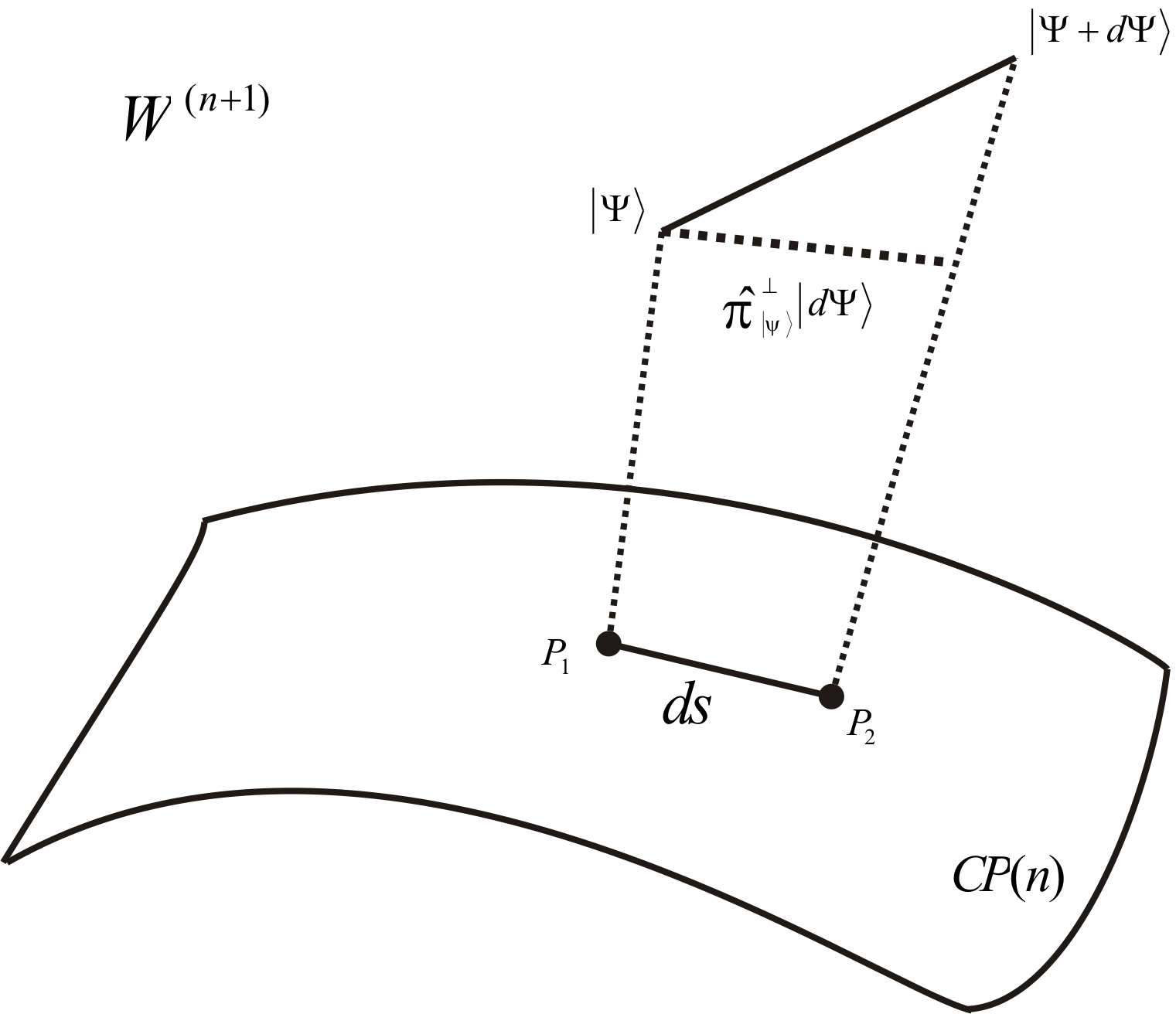
Figure 1: Pictorial representation of the quantum space of states.

The points $P_{1}$ and $P_{2}\in\mathbb{CP}(N)$ are the projections respectively from two infinitesimally nearby normalized state vectors $\left|\psi\right\rangle$ and $\left|\psi+d\psi\right\rangle$. It is natural to define then, the squared distance between $P_{1}$ and $P_{2}$ as the projection of $\left|d\psi\right\rangle$ in the subspace orthogonal to $\left|\psi\right\rangle$, that is, the projection given by the projective operator $\hat{\pi}_{\left|\psi\right\rangle}=\hat{I}-\left|\psi\right\rangle\left\langle\psi\right|$. It is then easy to see that

$$ds^{2}(\mathbb{CP}(N))=\left\langle d\psi\right|d\psi\rangle-\left\langle d\psi\right|\psi\rangle\left\langle\psi\right|d\psi\rangle$$ (43)

which is an elegant and coordinate independent manner to express the metric over $\mathbb{CP}(N)$. The time-evolution of a physical state in $\mathbb{CP}(N)$ is given by the projection of the linear Schrödinger evolution in $W^{(N+1)}$ which results in a Hamiltonian (classical-like) evolution in the space of rays.

5 Coherent States and the Quantum Symplectic Group

(The main references for this section are gilmore ; perelomov ; klauder ; combescure )

5.1 The Spectrum of the Fourier Transform Operator

Let $\hat{a}$ and $\hat{a}^{{\dagger}}$ be respectively the usual annihilation and creation operators defined as sakurai

$$\hat{a}=\frac{1}{\sqrt{2}}(\hat{Q}+i\hat{P})\qquad\text{and}\qquad\hat{a}^{{\dagger}}=\frac{1}{\sqrt{2}}(\hat{Q}-i\hat{P})$$ (44)

It follows immediately from the Heisenberg commutation relations that $[\hat{a},\hat{a}^{{\dagger}}]=\hat{I}$, and if we define also the hermitian number operator $\hat{N}=\hat{a}^{{\dagger}}\hat{a}$, it is not difficult to derive the well-known relations:

$$[\hat{N},\hat{a}]=-\hat{a}\qquad\text{and}\qquad[\hat{N},\hat{a}^{{\dagger}}\ ]=\hat{a}^{{\dagger}}$$ (45)

which implies the also well-known spectrum $\hat{N}\left|n\right\rangle=n\left|n\right\rangle$$(n=0,1,2,\ldots)$ of the number operator and the “up and down-the-ladder” action for $\hat{a}$ and $\hat{a}^{{\dagger}}$:

$$\hat{a}\left|n\right\rangle=\sqrt{n}\left|n\right\rangle\quad\text{and}\quad\hat{a}^{{\dagger}}\left|n\right\rangle=\sqrt{n+1}\left|n+1\right\rangle$$ (46)

and also where the ground-state or vacuum state $\left|0\right\rangle$ is annihilated by $\hat{a}$:

$$\hat{a}\left|0\right\rangle=0$$ (47)

The above algebraic equation for the vacuum state can be written in the position and momentum basis as the following differential equations:

$$\langle q(x)|\hat{a}|0\rangle =\frac{1}{\sqrt{2}}(x+\frac{d}{dx})\left\langle q(x)\right|0\rangle=\langle p(x)|\hat{a}|0\rangle$$

$$=\frac{1}{\sqrt{2}}(x+\frac{d}{dx})\left\langle p(x)\right|0\rangle=0$$ (48)

Which gives us the normalized Gaussian functions

$$\left\langle q(x)\right|0\rangle=\left\langle p(x)\right|0\rangle=\pi^{-1/4}e^{-x^{2}/2}$$ (49)

From equation (16) we conclude that the vacuum state is a fixed point of the Fourier Transform operator

$$\hat{F}|0\rangle=|0\rangle$$ (50)

The infinitesimal versions of equations (18) and (19) are simply

$$\hat{F}^{{\dagger}}\hat{a}\hat{F}=i\hat{a}\qquad\text{and}\qquad\hat{F}^{{\dagger}}\hat{a}^{{\dagger}}\hat{F}=-i\hat{a}^{{\dagger}}$$

Which implies that

$$[\hat{F},\hat{N}]=0$$

Thus, the Fourier transform operator commutes with the number operator so they necessarily share the same eigenstates. From the fixed point condition of the vacuum state together with the equations above, it is not difficult to see that

$$\hat{F}|n\rangle=(i)^{n}|n\rangle\qquad\text{and}\qquad\hat{F}=e^{i\frac{\pi}{2}\hat{N}},$$

which implies that $\hat{N}$ is the hermitian generator of the Fourier transform. In fact, at this point, it is a quite obvious move to introduce a complete rotation operator in phase space known as the Fractional Fourier Operator given by Namias

$$\hat{F}_{\theta}=e^{i\theta\hat{N}}$$

The Fourier transform operator is then recognized as a special case for $\theta=\pi/2$.

5.2 The Quantum Linear Symplectic Transforms

It is also natural to extend the Fractional Fourier transform to a complete set of quantum symplectic transforms, those unitary transformation in $W^{(\infty)}$ that implement a representation of the group of area preserving linear maps of the classical phase plane. This is the non-abelian $SL(2,\mathbb{R})$ group. Probably the best way to visualize this is through the identification of the phase plane with the complex plane via the standard complex-valued coherent states defined by the following change of variables: $z=(1/\surd 2)(q+ip)$ and by defining the coherent states as

$$|z\rangle=\hat{D}[z]|0\rangle\text{, with}\quad\hat{D}[z]=\frac{1}{2}\hat{\Delta}(z/2)\hat{F}^{2}=e^{(z\hat{a}^{{\dagger}}-z\hat{a})}$$ (51)

The $\hat{D}[z]$ operator is known as the displacement operator and the well-known “over-completeness” of the coherent state representation follows from the completeness of the $\hat{\Delta}(z)$ basis. The overlap between two arbitrary coherent states is given by

$$\left\langle z\right|z\prime\rangle=\left\langle p,q\right|p\prime,q\prime\rangle=e^{-1/4\left[(p-p\prime)^{2}+(q-q\prime)^{2}\right]}e^{i(p\prime q-pq\prime)/2}$$ (52)

Note above, the symplectic phase proportional to the area in the phase plane defined by the vectors $(p,q)$ and $(p\prime,q\prime)$. It is also not difficult to show that indeed

$$\hat{F}_{\theta}|z\rangle=e^{i\theta\hat{N}}|z\rangle=|e^{i\theta}z\rangle,$$ (53)

which is a direct manner to represent the Fractional Fourier transform for arbitrary $\theta$. Since the generator of rotations is quadratic in the canonical observables $\hat{Q}$ and $\hat{P}$, one may try to write down all possible quadratic operators in these variables: $\hat{Q}^{2},\hat{P}^{2},\hat{Q}\hat{P}$ and $\hat{P}\hat{Q}$, but the last two are obviously non-Hermitian so we could change them to the following (Hermitian) linear combinations: $\hat{Q}\hat{P}+\hat{P}\hat{Q}$ and $i(\hat{Q}\hat{P}-\hat{P}\hat{Q})$. The last one is proportional to the identity operator because of the Heisenberg commutation relation, so this leaves us with three linear independent operators that we choose as

$$\hat{H}_{0}=\frac{1}{2}(\hat{Q}^{2}+\hat{P}^{2})=\hat{N}+\frac{1}{2}\hat{I}=\hat{a}^{{\dagger}}\hat{a}+\frac{1}{2}\hat{I}$$ (54)

$$\hat{g}=\frac{1}{2}\{\hat{Q},\hat{P}\}=\frac{1}{2}(\hat{Q}\hat{P}+\hat{P}\hat{Q})=\frac{i}{2}[(\hat{a}^{{\dagger}})^{2}-\hat{a}^{2}]$$ (55)

$$\hat{k}=\frac{1}{2}(\hat{Q}^{2}-\hat{P}^{2})=\frac{1}{2}[(\hat{a}^{{\dagger}})^{2}+\hat{a}^{2}]$$ (56)

These three generators implement in $W^{(\infty)}$, the algebra $sl(2,\mathbb{R})$ of $SL(2,\mathbb{R})$. The $\hat{g}$ operator is nothing but the squeezing generator from quantum optics vedral . Indeed, the scale operator

$$\hat{S}_{\xi}=e^{i\hat{g}\ln\xi}$$ (57)

generated by $\hat{g}$ act upon the position and momentum basis respectively as

$$\hat{S}_{\xi}|q(x)\rangle=\sqrt{\xi}|q(\xi x)\rangle\quad\text{and}\quad\hat{S}_{\xi}|p(x)\rangle=\frac{1}{\sqrt{\xi}}|p(x/\xi)\rangle$$

The $\hat{k}$ operator generates hyperbolic rotations, that is, linear transformations of the plane that preserve an indefinite metric. It takes the hyperbola $x^{2}-y^{2}=1$ into itself in an analogous way that the Euclidean rotation takes the circle $x^{2}+y^{2}=1$ into itself. $SL(2,\mathbb{R})$ is the Lie Group of all area preserving linear transformations of the plane, so we can identify it with the $2\times 2$ real matrices with unit determinant. Since $\det e^{X}=e^{trX}$, we can also identify the algebra $sl(2,\mathbb{R})$ with all $2\times 2$ real matrices with null trace. Thus, it is natural to make the following choice for a basis in this algebra:

$$\begin{array}[]{c}\hat{X}_{1}=\hat{\sigma}_{1}\\ \hat{X}_{2}=i\hat{\sigma}_{2}\\ \hat{X}_{3}=\hat{\sigma}_{3},\end{array}$$

where we have written (for practical purposes) the elements of the algebra in terms of the well-known Pauli matrices. This is very adequate because physicists are familiar with the commutation relations of the Pauli matrices since they form a two-dimensional representation of the angular momentum algebra and we can make use of these algebraic relations to completely characterize the $sl(2,\mathbb{R})$ algebra. In fact, the mapping described by the table below relates these algebra elements directly to the algebra of their representation carried on $W^{(\infty)}$):

$$\begin{array}[]{cc}\text{{\small{Generators of }}}sl(2,\mathbb{R})&\text{{\small{\ Generators of the representation}}}\\ \hat{X}_{1}=\hat{\sigma}_{1}&-i\hat{k}\\ \hat{X}_{2}=i\hat{\sigma}_{2}&-i\hat{H}_{0}\\ \hat{X}_{3}=\hat{\sigma}_{3}&-i\hat{g}\end{array}$$ (58)

With a bit of work, it is not difficult to convince oneself that these mapped elements indeed obey identical commutation relations.

6 Weak Values and Quantum Mechanics in Phase Space

The weak value of a quantum system was introduced by Aharonov, Albert and Vaidman (A.A.V.) in AharonovAlbertVaidman based on the two-state formalism for Quantum Mechanics AharonovBergmannLebowitz ; AharonovVaidman and it generalizes the concept of an expectation value for a given observable. Let the initial state of a product space $W=W_{S}\otimes W_{M}$ be given by the product state $|\Psi\rangle=|\alpha\rangle\otimes|\phi_{(I)}\rangle$ where $|\alpha\rangle$ is the pre-selected state of the system and $|\phi_{(I)}\rangle$ is the initial state of the apparatus. Suppose further that a “weak Hamiltonian” governs the interaction between the system and the measuring apparatus as:

$$\hat{H}_{int}=\epsilon\delta(t-t_{0})\hat{O}\otimes\hat{P}\qquad(\epsilon\rightarrow 0),$$ (59)

where $\hat{O}$ is an arbitrary observable to be measured in the system. After the ideal instantaneous interaction that models this von Neumann (weak) measurement vonNeumann , suppose we post-select a certain final state $|\beta\rangle$ of the system after performing a strong measurement on it. In this case, the final state of the apparatus is clearly given by

$$|\phi_{(F)}\rangle =(\left\langle\beta\right|\otimes\hat{I})e^{-i\epsilon\hat{O}\otimes\hat{P}}(|\alpha\rangle\otimes|\phi_{(I)}\rangle)$$

$$\approx\left\langle\beta\right|\alpha\rangle(1-i\epsilon O_{w})|\phi_{(I)}\rangle,$$ (60)

where

$$O_{w}=\frac{\left\langle\beta\right|\hat{O}|\alpha\rangle}{\left\langle\beta\right|\alpha\rangle}$$ (61)

is the weak value of the observable $\hat{O}$ for these particular chosen pre and post-selected states. Note that the weak value $O_{w}$ of the observable is, in general, an arbitrary complex number. Note also that, though $|\phi_{(I)}\rangle$ is a normalized state, the $|\phi_{(F)}\rangle$ state vector in general, is not normalized. In the original formulation of (A.A.V.), the momentum $\hat{P}$ acts upon the measuring system, implementing a small translation of the initial wave function in the position basis, but which can be measured from the mean value of the results of a large series of identical experiments. That is, the expectation value of the position operator $\hat{Q}$ over a large ensemble with the same pre and post selected states. One can generalize this procedure jozsa by taking an arbitrary operator $\hat{M}$ in the place of $\hat{Q}$ as the observable of $W_{(M)}$ to be measured. In this case, the usual expectation values of $\hat{M}$ for the initial and final states $|\phi_{(I)}\rangle$ and $|\phi_{(F)}\rangle$ are respectively:

$$\langle\hat{M}\rangle_{(I)}=\langle\phi_{(I)}|\hat{M}|\phi_{(I)}\rangle\qquad\text{and}$$

$$\langle\hat{M}\rangle_{(F)}=\frac{\langle\phi_{(F)}|\hat{M}|\phi_{(F)}\rangle}{\langle\phi_{(F)}|\phi_{(F)}\rangle}$$ (62)

and the difference between these expectation values (the shift of $\hat{M}$) to first order in $\epsilon$ is given in general by jozsa :

$$\Delta\hat{M} =\langle\hat{M}\rangle_{(F)}-\langle\hat{M}\rangle_{(I)}$$

$$=\epsilon[(\operatorname{Im}(O_{w})(\langle\phi_{(I)}|\{\hat{M},\hat{P}\}|\phi_{(I)}\rangle-$$

$$-2\langle\phi_{(I)}|\hat{P}|\phi_{(I)}\rangle\langle\phi_{(I)}|\hat{M}|\phi_{(I)}\rangle)-$$

$$-i\operatorname{Re}(O_{w})\langle\phi_{(I)}|[\hat{M},\hat{P}]|\phi_{(I)}\rangle]$$ (63)

For the choice $\hat{M}=\hat{Q}$ and also by using the Heisenberg picture for the time evolution and by choosing the most general Hamiltonian $\hat{H}=\frac{1}{2m}\hat{P}^{2}+V(\hat{Q})$ for the measuring system one can derive the following shift (also using the $sl(2,\mathbb{R})$ algebra and the Heisenberg commutation relation):

$$\Delta\hat{Q}=\epsilon[\operatorname{Re}(O_{w})+m\operatorname{Im}(O_{w})\frac{d}{dt}(\delta_{|\phi_{(I)}\rangle}^{2}\hat{Q})],$$ (64)

where $\delta_{|\phi_{(I)}\rangle}\hat{Q}$ is the uncertainty of the initial state $|\phi_{(I)}\rangle$ and analogously for $\hat{M}=\hat{P}$, one arrives at

$$\Delta\hat{P}=2\epsilon\operatorname{Im}(O_{w})(\delta_{|\phi_{(I)}\rangle}^{2}\hat{P})$$ (65)

This result is clearly asymmetric because of the choice of the translation generator $\hat{P}$ in the interaction Hamiltonian. Note also that from the above equations one can see that it is impossible to extract the real and imaginary values of the weak value with the measurement of $\Delta\hat{Q}$ only, because both of these numbers are absorbed in a same real number. It is necessary to measure $\Delta\hat{P}$ (besides knowing the values of $\frac{d}{dt}(\delta_{|\phi_{(I)}\rangle}^{2}\hat{Q})$ and $\delta_{|\phi_{(I)}\rangle}^{2}\hat{P}$. There is no reason why one should need to choose $\hat{P}$ or $\hat{Q}$ in the weak measurement Hamiltonian. One may choose any of the symplectic generators making use of the full symmetry of the $SL(2,\mathbb{R})$ group. The $\hat{P}$ and $\hat{Q}$ operators generate translations in phase space, but one can implement any area preserving transformation in the plane by also using observables that are quadratic in the momentum and position observables. By making use of the freedom of choice of an arbitrary initial state vector $|\phi_{(i)}\rangle$ one can choose also an interaction Hamiltonian of the following form:

$$\hat{H}_{int}=\epsilon\delta(t-t_{0})\hat{O}\otimes\hat{R}\qquad(\epsilon\rightarrow 0),$$ (66)

where $\hat{R}$ is any element of the algebra $sl(2,\mathbb{R})$, so it is the generator of an arbitrary symplectic transform of the measuring system. In this way the generalized $\Delta\hat{M}$ shift in these conditions is given by:

$$\Delta\hat{M}= \epsilon\big{[}(\operatorname{Im}(O_{w})(\langle\phi_{(I)}|\{\hat{M},\hat{R}\}|\phi_{{}_{(I)}}\rangle-$$

$$-2\langle\phi_{{}_{(I)}}|\hat{R}|\phi_{{}_{(I)}}\rangle\langle\phi_{{}_{(I)}}|\hat{M}|\phi_{{}_{(I)}}\rangle)-$$

$$-i\operatorname{Re}(O_{w})\langle\phi_{{}_{(I)}}|[\hat{M},\hat{R}]|\phi_{{}_{(I)}}\rangle\big{]}$$

By making the choice $\hat{M}=\hat{R}$, one arrives at:

$$\Delta\hat{R}=2\epsilon\operatorname{Im}(O_{w})(\delta_{|\phi_{{}_{(I)}}\rangle}^{2}\hat{R})$$

For the second observable, we could choose any observable that does not commute with $\hat{R}$. This is because the main idea is to choose a “conjugate” variable to $\hat{R}$ in a similar way that occurs with the $(\hat{Q},\hat{P})$ pair. So one obvious choice is to pick the number operator $\hat{N}$ in the place of $\hat{R}$. Since $\hat{N}$ is the generator of Euclidean rotations in phase space, the annihilator operator $\hat{a}$ seems a natural candidate operator (though not hermitian) to go along with $\hat{N}$. With this choice of $\hat{M}=\hat{a}$ it is not difficult to calculate the shift for the annihilator operator:

$$\Delta\hat{a} =\epsilon[-iO_{w}\langle\phi_{{}_{(I)}}|\hat{a}|\phi_{{}_{(I)}}\rangle+2\operatorname{Im}(O_{w})(\langle\phi_{{}_{(I)}}|\hat{N}\hat{a}|\phi_{{}_{(I)}}\rangle-$$

$$-\langle\phi_{{}_{(I)}}|\hat{N}|\phi_{{}_{(I)}}\rangle\langle\phi_{{}_{(I)}}|\hat{a}|\phi_{{}_{(I)}}\rangle)]$$ (67)

In most models of weak measurements, the initial state of the measuring system is chosen to be a Gaussian state and the weak interaction promotes a small translation of its center. In realistic quantum optical implementations of the measuring system, it is reasonable to choose the initial state of the system as a coherent state $|\phi_{{}_{(I)}}\rangle=|z\rangle$. In this case, there is a dramatic simplification for the shift:

$$\Delta\hat{a}=i\epsilon O_{w}=\epsilon|O_{w}|e^{i(\theta_{z}+\theta_{w}-\pi/2)}$$

where $z=|z|e^{i\theta_{z}}$ and $O_{w}=|O_{w}|e^{i\theta_{w}}$. If we make the following convenient choice for the phase $\theta_{z}=\pi/2$ and rewrite the above equation in terms of the canonical pair $(\hat{Q},\hat{P})$, we arrive at a symmetric pair of equations for $\Delta\hat{Q}$ and $\Delta\hat{P}$:

$$\Delta\hat{Q}=\epsilon\sqrt{2}|z|\operatorname{Re}(O_{w})\quad\text{and}\quad\Delta\hat{P}=\epsilon\sqrt{2}|z|\operatorname{Im}(O_{w})$$ (68)

These equations do not depend on the quadratic dispersion or the time derivative of the quadratic dispersion of any observable for the initial state of the measuring system and, in principle, one may “tune” the size of the $\epsilon|z|$ term despite how small $\epsilon$ may be by making $|z|$ large enough. This is of great practical importance for optical implementations of weak value measurements since $|z|$ for a quantized mode of an electromagnetic field is nothing else but the mean photon number in this mode for the coherent state $|z\rangle$ vedral .

7 von Neumann’s Pre-measurement, Weak Values and the Geometry of Quantum Mechanics

In the last section we discussed von Neumann’s model for a pre-measurement in the weak measurement limit in order to obtain a deeper understanding of the concept of a weak value in terms of a quantum phase space analysis of the measuring apparatus system. In this section we implement, in a certain sense, the opposite approach: We shall discuss certain geometric structures of the measured system based on previous work of Tamate et al Tamate . Let $W=W_{(S)}\otimes W_{(M)}$ be the state space formed by composing the subsystem $W_{(S)}$ with the measuring subsystem $W_{(M)}$. We will initially assume that the measured system is a discrete quantum variable of $W_{(S)}$ defined by an observable $\hat{O}=|o_{k}\rangle o_{k}\langle o^{k}|$ (we use henceforth the sum convention). The measuring subsystem will be considered as a structure-less (no spin or internal variables) quantum mechanical particle in one dimension (further ahead we will also consider discrete measuring systems). Suppose the initial state of the total system is given by the following unentangled product state: $|\Psi_{(I)}\rangle=|\alpha\rangle\otimes|\phi_{(I)}\rangle$. After performing an ideal von Neumann measurement through the interaction Hamiltonian,

$$\hat{H}_{int}=\lambda\delta(t-t_{0})\hat{O}\otimes\hat{P}$$ (69)

the final state will be

$$(\hat{I}\otimes\langle q(x)|)|\Psi_{(F)}\rangle=|o_{j}\rangle\alpha^{j}\phi_{(I)}(x-\lambda o_{j}),$$

where $\phi_{(I)}(x)=\left\langle q(x)\right|\phi_{(I)}\rangle$ is the initial wave-function in the position basis of the measuring system. Note that a correlation in the final state of the total system is then established between the variable to be measured $o_{j}$ with the continuous position variable of the measuring particle. This step of the von Neumann measurement prescription is called the pre-measurement of the system.

Consider now the measuring system as a finite dimensional quantum system $W_{(M)}$. In particular, if $n=2$, our measuring apparatus consists of a single qubit so that we can treat this two-level measuring system making explicit use of the $\mathbb{CP}(1)$ (Bloch sphere) geometry. A single qubit can be written in the Bloch sphere standard form as

$$|\theta,\phi\rangle=\cos(\theta/2)|u_{0}\rangle+e^{i\phi}\sin(\theta/2)|u_{0}\rangle$$ (70)

The single projective coordinate in this case is $\xi=\tan(\theta/2)e^{i\phi}$ and, remarkably, we shall see that this complex number can actually be measured physically as a certain appropriate weak value for two level systems. Suppose now that the interaction happens in an arbitrary finite dimensional measuring system: $W=W_{(S)}\otimes W_{(M)}$, that is, $\dim W_{(M)}=m$. The initial non-entangled pure-state is $|\Psi_{(I)}\rangle=|\alpha\rangle\otimes|\phi_{(I)}\rangle$ and the finite momentum basis is given by $\{|v_{\sigma}\rangle\},(\sigma=0,1,\ldots,m-1)$ so that the momentum observable can be expressed as $\hat{P}=|v_{\sigma}\rangle p_{\sigma}\left\langle v^{\sigma}\right|$. Again we model our instantaneous interaction with the interaction Hamiltonian given by (69) so that our final entangled state is given by

$$|\Psi_{(F)}\rangle=|A_{\sigma}\rangle\otimes|v_{\sigma}\rangle\phi^{\sigma},$$ (71)

where

$$|A_{\sigma}\rangle=e^{-i\lambda p_{\sigma}\hat{O}}|\alpha\rangle\qquad\text{and}\qquad|\phi_{(I)}\rangle=|v_{\sigma}\rangle\phi^{\sigma}$$ (72)

The above entangled state clearly establishes a finite index correlation between $|A_{\sigma}\rangle\in W_{(S)}$ and the finite momentum basis $|v_{\sigma}\rangle$. The total system is in the pure state $|\Psi_{(F)}\rangle\langle\Psi_{(F)}|$ and by tracing out the first subsystem, the measuring system will be:

$$\hat{\rho}_{|\Psi_{(F)}\rangle}=|v_{\sigma}\rangle\phi^{\sigma}\left\langle A^{\sigma}\right|A_{\tau}\rangle\phi_{\tau}\left\langle A^{\tau}\right|$$ (73)

For a single qubit, one has

$$|\phi_{(I)}\rangle=\cos(\theta/2)|v_{0}\rangle+e^{i\phi}\sin(\theta/2)|v_{1}\rangle,$$ (74)

with

$$\langle A^{0}|A_{1}\rangle=|\langle A^{0}|A_{1}\rangle|e^{-i\eta}$$ (75)

so that we can compute the probability $P(\eta)$ of finding the second subsystem in a certain reference state $|\theta=\pi/2,\varphi=0\rangle$ as

$$P(\eta) =tr(\hat{\rho}_{|\Psi_{(F)}\rangle}|\pi/2,0\rangle\langle\pi/2,0|)$$

$$=\frac{1}{2}+\frac{1}{4}\left(|\langle A^{0}|A_{1}\rangle|\sin\theta\cos(\phi-\eta)\right)$$ (76)

For a fixed $\theta$, this probability is clearly maximized when $\mathit{\phi=\eta}$. This fact can be used to measure the so called geometric phase

$$\eta=\arg\langle A^{0}|A_{1}\rangle$$

between the two indexed states $|A_{0}\rangle$ and $|A_{1}\rangle\in W_{(S)}$. This definition of a geometric phase was originally proposed in 1956 by Pancharatnam pancharatnam for optical states and rediscovered by Berry in 1984 berry in his study of the adiabatic cyclic evolution of quantum states. In 1987, Anandan and Aharonov aharonovanandan1987 gave a description of this phase in terms of natural geometric structures of the $U(1)$ fiber-bundle structure over the space of rays and of the symplectic and Riemannian structures in the projective space $\mathbb{CP}(N)$ inherited from the hermitian structure of $W_{(S)}$.

Given the final state $|\Psi_{(F)}\rangle$, one may then “post-select” a chosen state $|\beta\rangle\in W_{(S)}$. The resulting state is then clearly

$$|\Psi_{(F)}\rangle=C(\left|\beta\right\rangle\left\langle\beta\right|\otimes\hat{I}))\left(\left|A_{\sigma}\right\rangle\otimes\left|v_{\sigma}\right\rangle\phi^{\sigma}\right),$$ (77)

where $C$ is an unimportant normalization factor. Because of the post-selection, the system is now again in a non-entangled state so that the partial trace of $|\Psi_{(F)}\rangle\langle\Psi_{(F)}|$ over the first subsystem gives us

$$|\phi_{(F)}\rangle=C\langle\beta|A^{0}\rangle\left|v_{\sigma}\right\rangle\phi^{\sigma}$$ (78)

By making the following phase choices

$$\left\langle\beta\right|A^{0}\rangle=|\langle\beta|A^{0}\rangle|e^{i\beta_{0}}\quad\text{and}\quad\left\langle\beta\right|A^{1}\rangle=|\langle\beta|A^{1}\rangle|e^{-i\beta_{1}}$$ (79)

we can again compute the probability of finding the second subsystem in state $\left|\pi/2,0\right\rangle$ and again one finds that for a fixed angle $\theta$, the maximum probability occurs for

$$\phi\prime=\beta_{0}+\beta_{1}=\arg(\left\langle\beta\right|A_{0}\rangle\left\langle A^{1}\right|\beta\rangle)$$ (80)

This implies that there is an overall phase change $\Theta$ given by

$$\Theta=\phi\prime-\phi=\arg(\left\langle A^{1}\right|\beta\rangle\left\langle\beta\right|A^{0}\rangle\left\langle A^{0}\right|A^{1}\rangle),$$ (81)

which is a well-known geometric invariant in the sense that it depends only on the projection of the state-vectors $\left|A_{0}\right\rangle$, $\left|A_{1}\right\rangle$ and $\left|\beta\right\rangle$ on the Bloch sphere. In fact, this quantity is the intrinsic geometric phase picked by a state-vector that is parallel transported through the closed geodesic triangle defined by the projection of the three states on the space of rays. For a single qubit, the geometric invariant is proportional to the area of the geodesic triangle formed by the projection of the kets $\left|A_{0}\right\rangle$, $\left|A_{1}\right\rangle$ and $\left|\beta\right\rangle$ on the Bloch sphere and it is well known to be given by

$$\Theta=\arg(\left\langle A^{1}\right|\beta\rangle\left\langle\beta\right|A^{0}\rangle\left\langle A^{0}\right|A^{1}\rangle)=-\Omega/2,$$ (82)

where $\Omega$ is the oriented solid angle formed by the geodesic triangle.

Figure 2: Solid angle formed by N. Pole and 2 Equator points.

Returning to the single qubit case, notice that if we choose the following state $\left|\alpha\right\rangle=\left|u_{0}\right\rangle$ for the pre-selected state (the “north pole” of the Bloch sphere), and $|\theta,\phi\rangle$ for the post-selected state and also

$$\hat{O}=\hat{\sigma}_{1}=\left|u_{0}\right\rangle\left\langle u^{1}\right|+\left|u_{1}\right\rangle\left\langle u^{0}\right|$$ (83)

as the observable, then it is straightforward to compute the weak value as

$$O_{w}=\tan(\theta/2)e^{i\phi},$$ (84)

which is clearly complex-valued in general. What is curious about this result is that the weak value gives a direct physical meaning to the complex projective coordinate of the state vector in the Bloch sphere given by (40) kobayashi2013 .

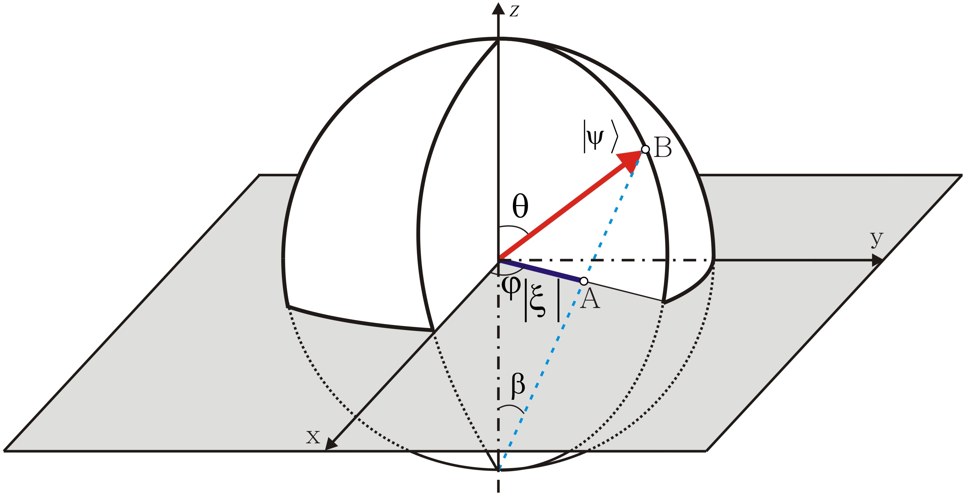
Figure 3: Stereographic projection.

Suppose now that the physical system $W$ is composed by two subsystems $W_{(S)}\otimes W^{(\infty)}$ as before, but the measuring system $W^{(\infty)}$ is spanned by a complete basis of position kets $\{\left|q(x)\right\rangle\}$ (momentum kets $\{\left|p(x)\right\rangle\}$), with $-\infty<x,y<+\infty$. And again let us consider the initial state as the product state vector $|\Psi_{(I)}\rangle=|\alpha\rangle\otimes|\phi_{(I)}\rangle$ together with an instantaneous interaction coupling the observable $\hat{O}$ of $W_{(S)}$ with the momentum observable $\hat{P}$ in $W^{(\infty)}$. The system evolves then to

$$|\Psi_{(F)}\rangle=\int_{-\infty}^{+\infty}dy\left|A(y)\right\rangle\otimes\left|p(y)\right\rangle\widetilde{\phi}_{(I)}(y),$$ (85)

where

$$\left|A(y)\right\rangle=e^{-i\lambda y\hat{O}}\left|\alpha\right\rangle$$ (86)

is the continuous indexed states that are correlated to the momentum basis of the measuring apparatus and

$$\widetilde{\phi}_{(I)}(y)=\left\langle p(y)\right|\phi_{(I)}\rangle$$ (87)

is the wave function of the initial state of the apparatus in the momentum basis. We may now compute (to first order in $dy$) the intrinsic phase shift between $\left|A(y)\right\rangle$ and $\left|A(y+dy)\right\rangle$ in a similar manner that was carried out before with the discretely parameterized states:

$$\arg(\left\langle A(y)\right|A(y+dy)\rangle)\approx-\lambda dy\langle\hat{O}\rangle_{\left|\alpha\right\rangle},$$ (88)

where $\langle\hat{O}\rangle_{\left|\alpha\right\rangle}$ is the expectation value

$$\langle\hat{O}\rangle_{\left|\alpha\right\rangle}=\left\langle\alpha\right|\hat{O}\left|\alpha\right\rangle$$ (89)

is the expectation value of observable $\hat{O}$ in the initial state $\left|\alpha\right\rangle$. We can also compute the shift of the expectation value of the position observable of the particle of the measuring system between the initial and final states. Let $\{\left|o_{j}\right\rangle\},\ (j=0,1,\ldots N-1)$ be a complete set of eigenkets of observable $\hat{O}$. The final state of the composite system can be described by the following pure density matrix:

$$\hat{\rho}_{|\Psi(F)\rangle} =|\Psi_{(F)}\rangle\langle\Psi_{(F)}|$$

$$=|o_{j}\rangle\langle o^{k}|\otimes\alpha^{j}\hat{V}_{\lambda o_{j}}^{{\dagger}}|\phi_{(I)}\rangle\langle\phi_{(I)}|\hat{V}_{\lambda o_{k}}\alpha_{k}$$ (90)

By taking the partial trace of the $W_{(S)}$ system, we arrive at the following mixed state that describes the measuring system at instant $t_{F}$:

$$\hat{\rho}_{\left|\Psi(F)\right\rangle}^{(M)}=\underset{j}{\sum}|\alpha_{j}|^{2}\hat{V}_{\lambda o_{j}}^{{\dagger}}\left|\phi_{(I)}\right\rangle\left\langle\phi_{(I)}\right|\hat{V}_{\lambda o_{j}}$$ (91)

The ensemble expectation value of position is then

$$[\hat{Q}]_{\hat{\rho}_{\left|\Psi(F)\right\rangle}^{(M)}}=tr(\hat{\rho}_{\left|\Psi(F)\right\rangle}^{(M)}\hat{Q})=\langle\hat{Q}\rangle_{|\phi_{(I)}\rangle}+\lambda\langle\hat{O}\rangle_{\left|\alpha\right\rangle}$$

A geometric interpretation of this von Neumann’s pre-measurement can be presented in the following way: Let $\left|\psi(t)\right\rangle$ be the curve of normalized state vectors in $W^{(N+1)}$ given by the unitary evolution generated by a given Hamiltonian $\hat{H}(t)$. The Schrödinger equation implies a relation between $\left|\psi(t)\right\rangle$ and $\left|\psi(t+dt)\right\rangle$ given by:

$$\left|d\psi(t)\right\rangle=\left|\psi(t+dt)\right\rangle-\left|\psi(t)\right\rangle=-i\hat{H}\left|\psi(t)\right\rangle dt$$

The above equation together with (43) lead to a very elegant relation for the squared distance between two infinitesimally nearby projection of state vectors connected by the unitary evolution over $\mathbb{CP}(N)$ aharonovanandan1987 :

$$ds^{2}(\mathbb{CP}(N)) =[\left\langle\psi(t)\right|\hat{H}^{2}\left|\psi(t)\right\rangle-\left\langle\psi(t)\right|\hat{H}\left|\psi(t)\right\rangle^{2}]dt^{2}$$

$$=\delta_{\left|\psi(t)\right\rangle}^{2}E$$ (92)

The above equation means that the speed of the projection over $\mathbb{CP}(N)$ equals the instantaneous energy uncertainty

$$\frac{ds}{dt}=\delta_{\left|\psi(t)\right\rangle}E$$ (93)

A beautiful geometric derivation of the time-energy uncertainty relation that follows directly from this equation can be found in aharonovanandan1987 . (See also loboribeiroribeiro for a pedagogical discussion of this result related to the adiabatic theorem in quantum mechanics).

Back to our discussion of the interaction between the systems $W^{(S)}$ and $W^{(\infty)}$, note that the expression $\left|A(y)\right\rangle=e^{-i\lambda y\hat{O}}\left|\alpha\right\rangle$ is formally equivalent to the unitary time evolution equation $\left|\psi(t)\right\rangle=e^{-i\hat{H}t}\left|\psi(0)\right\rangle$ which is clearly a solution of the Schrödinger equation with a time-independent Hamiltonian. A formal analogy between the two distinct physical processes is exemplified by the association below:

$$\begin{array}[]{ll}|\psi(t)\rangle&\mapsto|A(y)\rangle\\ |\psi(0)\rangle&\mapsto|\alpha\rangle=|A(0)\rangle\\ t&\mapsto y\\ \hat{H}&\mapsto\lambda\hat{O}.\end{array}$$

Looking at subsystem $W^{(S)}$ and regarding $y$ as an external parameter (just like the time variable for the unitary time evolution) we may write the analog of (92) in $\mathbb{CP}(N)\subset W^{(S)}$:

$$ds^{2} =[\left\langle A(y)\right|\hat{O}^{2}\left|A(t)\right\rangle-\left\langle A(y)\right|\hat{O}\left|A(t)\right\rangle^{2}]\lambda^{2}dy^{2}$$

$$=[\left\langle\alpha\right|\hat{O}^{2}\left|\alpha\right\rangle-\left\langle\alpha\right|\hat{O}\left|\alpha\right\rangle^{2}]\lambda^{2}dy^{2}$$ (94)

Comparing this result with equations (43) and (88) we can immediately see the geometric interpretation for the expectation value $\left\langle\alpha\right|\hat{O}\left|\alpha\right\rangle$ in terms of the $U(1)$ fiber bundle structure as one can easily infer from the pictorial representation in Figure 4.

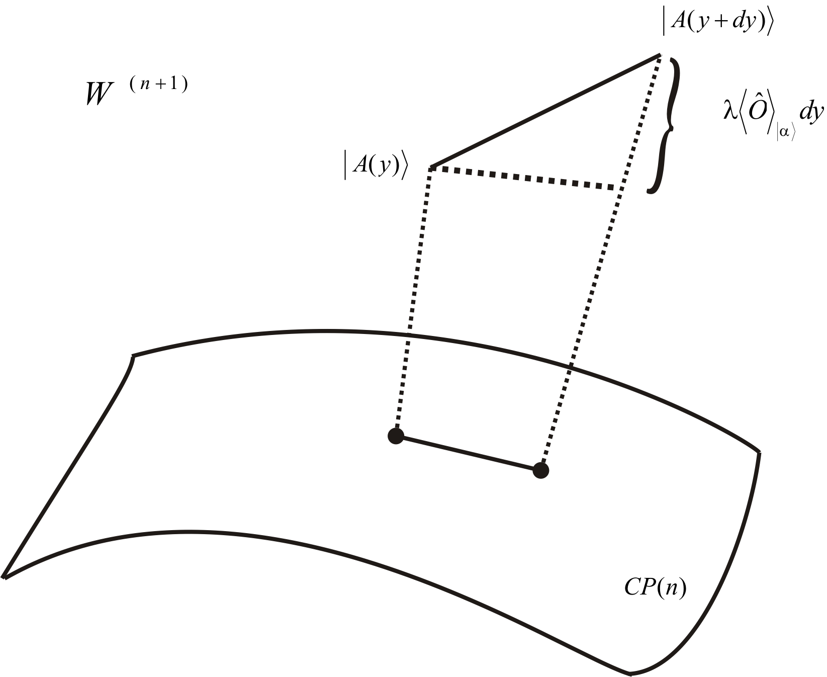
Figure 4: Phase difference between $|A(y)\rangle$ and  $|A(y+dy)\rangle$.

For the case of a weak measurement, we choose again the Hamiltonian given by equation (59). Given the initial unentangled state $|\Psi_{(I)}\rangle=|\alpha\rangle\otimes|\phi_{(I)}\rangle$ at $t_{0}$, the evolution of the system is described as

$$|\Psi_{(F)}\rangle=\int_{-\infty}^{+\infty}dy\left|A(y)\right\rangle\otimes\left|p(y)\right\rangle\widetilde{\phi}_{(I)}(y)\text{, with}$$

$$\left|A(y)\right\rangle=e^{-i\lambda y\hat{O}}\left|\alpha\right\rangle$$

The global geometric phase related to the infinitesimal geodesic triangle formed by the projections of $\left|A(y)\right\rangle$, $\left|A(y+dy)\right\rangle$ and the post-selected state $\left|\beta\right\rangle$ on $\mathbb{CP}(N)$ (see Figure 5) is clearly given by

$$\Theta=\arg(\left\langle A(y)\right|\beta\rangle\left\langle\beta\right|A(y+dy)\rangle\left\langle A(y+dy)\right|A(y)\rangle)$$ (95)

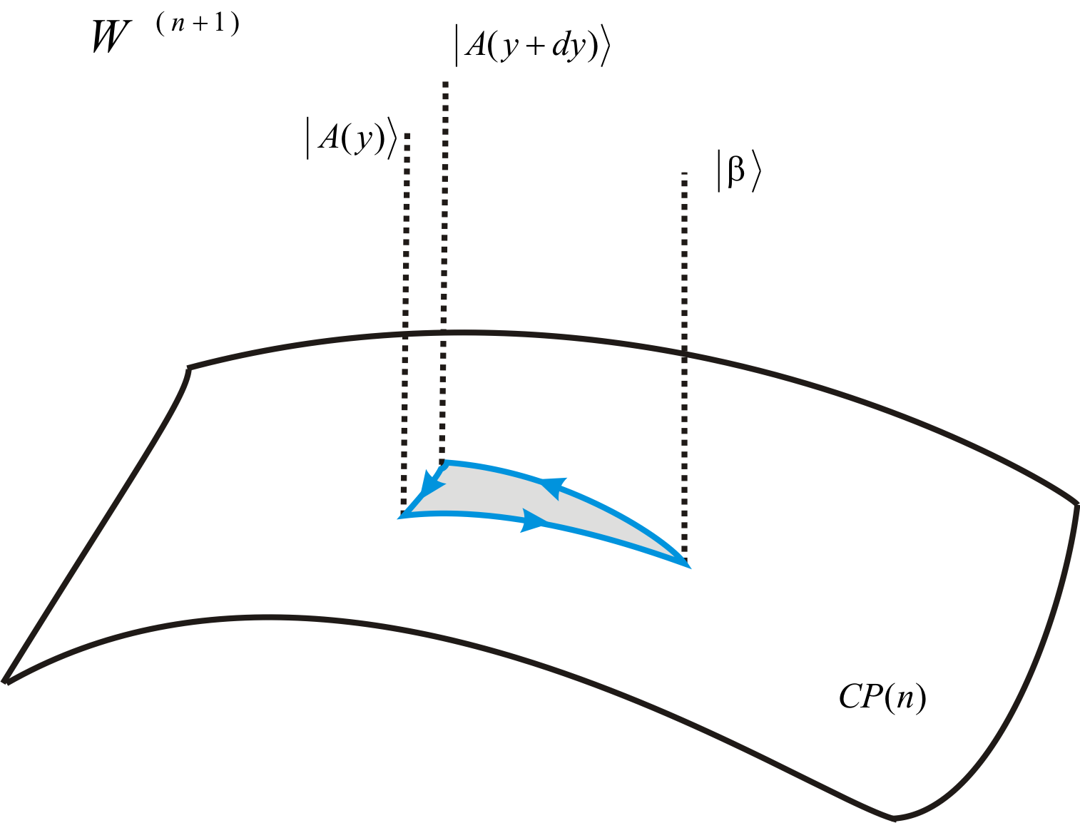
Figure 5: Representation of global geometric phase.

8 The Geometry of Deterministic Measurements

As is well-known, the collapse postulate of Quantum Mechanics implies that, in general, the measurement of a quantum state causes a disturbance of the state as the state “jumps” to an eigenstate of the observable that is being measured in a stochastic manner. Yet, if the state is already an eigenstate of the observable, then the state is left untouched. This is what is behind the notion of “deterministic” experiments. We call a measurement, a deterministic experiment when we measure only variables for which the state of the system under investigation is an eigenstate. In other words, for any state $\left|\psi\right\rangle$ it is possible to ask the following question: “What is the set of Hermitian operators $A_{\left|\psi\right\rangle}$ for which $\left|\psi\right\rangle$ is an eigenstate?” That is, which satisfy:

$$A_{\left|\psi\right\rangle}=\{\hat{A}_{i}\,\,\text{such\thinspace\thinspace that}\,\,\hat{A}_{i}|\psi\rangle=a_{i}|\psi\rangle\,,a_{i}\in\mathbf{\mathbb{R}}\}$$ (96)

One can think this as kind of a dual question to the more familiar inquire which asks “What are the eigenstates of a given operator?” The measurements of such operators $A_{\left|\psi\right\rangle}$ would not lead to any wave function collapse, since the wave function is initially an eigenstate of the operator being measured. The results are completely predictable and so the experiments are deterministic in this sense. Given $\left|\psi\right\rangle$, one can characterize mathematically in a very precise way the deterministic set of operators (DSO) $A_{\left|\psi\right\rangle}$. In fact, let $\hat{A}_{i},\hat{A}_{j}\in A_{\left|\psi\right\rangle}$, then the set $A_{\left|\psi\right\rangle}$ is closed in the sense that:

1. $[\hat{A}_{i},\hat{A}_{j}]\in A_{\left|\psi\right\rangle}$

2. $\alpha\hat{A}_{i}+\beta\hat{A}_{j}\in A_{\left|\psi\right\rangle}$ with $\alpha,\beta\in\mathbb{R}$

3. $\hat{A}_{i}\hat{A}_{j}$ $\in A_{\left|\psi\right\rangle}$

Note that $[\hat{A}_{i},\hat{A}_{j}]$ is a special deterministic operator in the sense that it annihilates $\left|\psi\right\rangle$, $[\hat{A}_{i},\hat{A}_{j}]\left|\psi\right\rangle=0$. This implies that $[\hat{A}_{i},\hat{A}_{j}]$ must be proportional to the projector $\hat{\Pi}_{\left|\psi\right\rangle}^{\perp}=\hat{I}-\hat{\Pi}_{\left|\psi\right\rangle}=\hat{I}-\left|\psi\right\rangle\left\langle\psi\right|$ that projects vectors to the subspace that is orthogonal to $\left|\psi\right\rangle$.

Note that the projector operators $\hat{\Pi}_{\left|\psi\right\rangle}$ and $\hat{\Pi}_{\left|\psi\right\rangle}^{\perp}$ are clearly idempotent, that is $\hat{\Pi}_{\left|\psi\right\rangle}^{2}=\hat{\Pi}_{\left|\psi\right\rangle}$ and $(\hat{\Pi}_{\left|\psi\right\rangle}^{\perp})^{2}=\hat{\Pi}_{\left|\psi\right\rangle}^{\perp}$.

Also, if we know the Hamiltonian $\hat{H}$ of the system, then we know the set $A_{\left|\psi(t)\right\rangle}$ for each instant of time, where $|\psi(t)\rangle$ is a solution of Schrödinger’s equation $\hat{H}|\psi(t)\rangle=i|\dot{\psi}(t)\rangle$.

If we have a Hilbert space of dimension $n$ then we can choose an orthonormal basis such that the state vector $|\psi\rangle$ can be represented by the $n\times 1$ column vector below (a unitary transformation can always bring us to such a basis) together with any orthogonal vector $|\psi_{\bot}\rangle$

$$|\psi\rangle=\left(\begin{array}[]{ccccc}1&0&0&\ldots&0\end{array}\right)^{T}\text{, and\quad}|\psi_{\bot}\rangle=\left(\begin{array}[]{ccccc}0&a^{1}&a^{2}&\ldots&a^{n}\end{array}\right)^{T}$$ (97)

The Hermitian operators that operate on a $n$-di- mensional space form an real $n^{2}$-dimensional algebra. The DSO that act upon this space (in the above basis) can be represented by

$$\left(\begin{array}[]{ccccc}a_{1}^{1}&0&0&\ldots&0\\ 0&a_{2}^{2}&a_{3}^{2}&\ldots&a_{n}^{2}\\ 0&a_{2}^{3}&a_{3}^{3}&\ldots&a_{3}^{3}\\ \vdots&\vdots&\vdots&\ddots&\vdots\\ 0&a_{2}^{n}&a_{3}^{n}&\ldots&a_{n}^{n}\end{array}\right)$$ (98)

with $a_{j}^{i}=\bar{a}_{i}^{j}$, so that the dimension of the DSO space is clearly $(n-1)^{2}+1$.

8.1 The Completely Uncertain Operators

In addition to the set $A_{\left|\psi\right\rangle}$ of DSO, there is also a set $B_{\left|\psi\right\rangle}$ of operators whose results are completely uncertain. In fact, given $\left|\psi\right\rangle$, we can always decompose any operator $\hat{C}$ in the following unique way:

$$\hat{C}\equiv\hat{A}_{\left|\psi\right\rangle}^{(C)}+\hat{B}_{\left|\psi\right\rangle}^{(C)}$$ (99)

where

$$\hat{A}_{\left|\psi\right\rangle}^{(C)}=\hat{\Pi}_{\left|\psi\right\rangle}\hat{C}\hat{\Pi}_{\left|\psi\right\rangle}+\hat{\Pi}_{\left|\psi\right\rangle}^{\perp}\hat{C}\hat{\Pi}_{\left|\psi\right\rangle}^{\perp}\text{, and}$$

$$\hat{B}_{\psi}^{(C)}=\hat{\Pi}_{\left|\psi\right\rangle}^{\perp}\hat{C}\hat{\Pi}_{\left|\psi\right\rangle}+\hat{\Pi}_{\left|\psi\right\rangle}\hat{C}\hat{\Pi}_{\left|\psi\right\rangle}^{\perp}$$ (100)

In the same basis of (98), the completely uncertain operators (CUO) have the following matrix form:

$$\hat{B}\left|\psi\right\rangle=\left(\begin{array}[]{ccccc}0&b_{2}^{1}&b_{3}^{1}&\ldots&b_{n}^{1}\\ b_{1}^{2}&0&0&\ldots&0\\ b_{1}^{3}&0&0&\ldots&0\\ \vdots&\vdots&\vdots&\ddots&\vdots\\ b_{n}^{3}&0&0&\ldots&0\end{array}\right)\left(\begin{array}[]{c}1\\ 0\\ 0\\ \vdots\\ 0\end{array}\right)=\left(\begin{array}[]{c}0\\ b_{1}^{2}\\ b_{1}^{3}\\ \vdots\\ b_{n}^{3}\end{array}\right)=\lambda\left|\psi_{\bot}\right\rangle$$ (101)

Note that the uncertain operator $\hat{B}$ takes the state $\left|\psi\right\rangle$ to an orthogonal normalized state $|\psi_{\bot}\rangle$ (up to a normalizing factor $\lambda$) and that the dimension of the CUO subspace of operator subspace is clearly $2(n-1)$. In this way, we see that the $n^{2}$-dimensional space of Hermitian operators is decomposed into the direct orthogonal sum of the DSO and CUO subspaces:

$$\dim(DSO\oplus CUO)=n^{2}=\dim(DSO)+\dim(CUO)$$ (102)

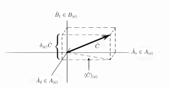
Figure 6: Pictorial representation in Operator Space.

Traditionally, it was believed that if a measurement interaction is weakened so that there is no disturbance on the system, then no information could be obtained. However, the advent of the concept of weak measurements and weak values has changed the point of view on this issue quite dramatically. Not only we have learned that there is indeed a gain of information, but it turned-out to be quite a very important tool both theoretically and for practical purposes Yutaka2012 ; dressel2014 .

It has been shown spie-nswm that information can be obtained even though not a single particle (in an ensemble) is disturbed. To begin to introduce this point, let us consider a general theorem for any vector in Hilbert space:

Theorem 8.1

Let $W$ be a Hilbert space and an arbitrary non-null normalized vector $|\psi\rangle\in W$ and also let $\hat{A}$ be an arbitrary Hermitian operator that acts upon $W$, then:

$$\hat{A}|\psi\rangle=\langle\hat{A}\rangle_{|\psi\rangle}|\psi\rangle+\delta_{|\psi\rangle}\hat{A}|\psi_{\perp}\rangle$$ (103)

where $\langle\hat{A}\rangle_{|\psi\rangle}=\left\langle\psi\right|\hat{A}|\psi\rangle$ is the expectation value of observable $\hat{A}$ in state $|\psi\rangle$, $\delta_{|\psi\rangle}^{2}\hat{A}=\left\langle\psi\right|\hat{A}^{2}|\psi\rangle-\left\langle\psi\right|\hat{A}|\psi\rangle^{2}$ is the squared uncertainty of observable $\hat{A}$ in state $|\psi\rangle$, and $|\psi_{\perp}\rangle$ is a vector that belongs to the subspace of $W$ that is orthogonal to $|\psi\rangle$.

Proof

Left multiplication by $\langle\psi|$ yields the first term. By using that $\hat{\Pi}_{\left|\psi\right\rangle}^{\perp}=|\psi_{\perp}\rangle\langle\psi_{\perp}|=\hat{I}-\hat{\Pi}_{\left|\psi\right\rangle}=\hat{I}-|\psi\rangle\langle\psi|$ and also by evaluating $|(\hat{A}-\langle\hat{A}\rangle_{|\psi\rangle}\hat{I})|\psi\rangle|^{2}=\delta_{|\psi\rangle}^{2}\hat{A}$ yields the second term.

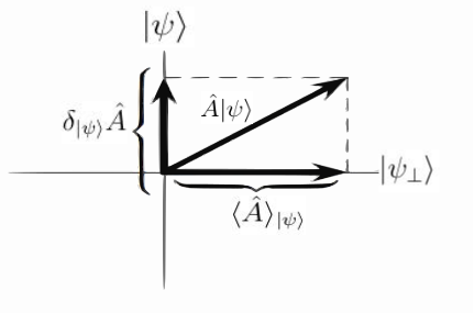
Figure 7: Pictorial Representation in Hilbert Space.

Using this theorem, it is easy to see that in the basis of eq. (97), the diagonal elements of (98) correspond to the averages of the observables, e.g. $a_{1}^{1}=\langle\hat{A}\rangle_{\left|\psi\right\rangle}$ for state $\left|\psi\right\rangle$, which again can be measured without uncertainty.

By normalizing the vector in the second member of eq. (101), one has for its square modulus

$$\lambda^{2}=|b_{1}^{2}|^{2}+|b_{1}^{3}|^{2}+\cdot\cdot+|b_{1}^{n}|^{2}$$ (104)

From the above theorem, it is also easy to see that the normalizing factor $\lambda$ in eq. (101) is nothing else but the uncertainty of $\hat{B}$:

$$\lambda=\delta_{\left|\psi\right\rangle}\hat{B}$$ (105)

8.2 Deterministic and Partially Deterministic Protocols

8.2.1 The Case of a Single qubit

Consider a quantum system represented by a single qubit as in the spin of a electron for instance. The best way to “visualize” this system is to represent its states on the Bloch sphere. Suppose that the north and south “poles” of the sphere are represented by the orthonormal basis $\left\{\left|u_{0}\right\rangle,\left|u_{1}\right\rangle\right\}$ and let

$$\left|\psi_{\alpha}\right\rangle=\frac{1}{\sqrt{2}}\left(\left|u_{0}\right\rangle+e^{i\alpha}\left|u_{1}\right\rangle\right)$$ (106)

be an arbitrary state represented on the “equator” of the sphere as in shown below:

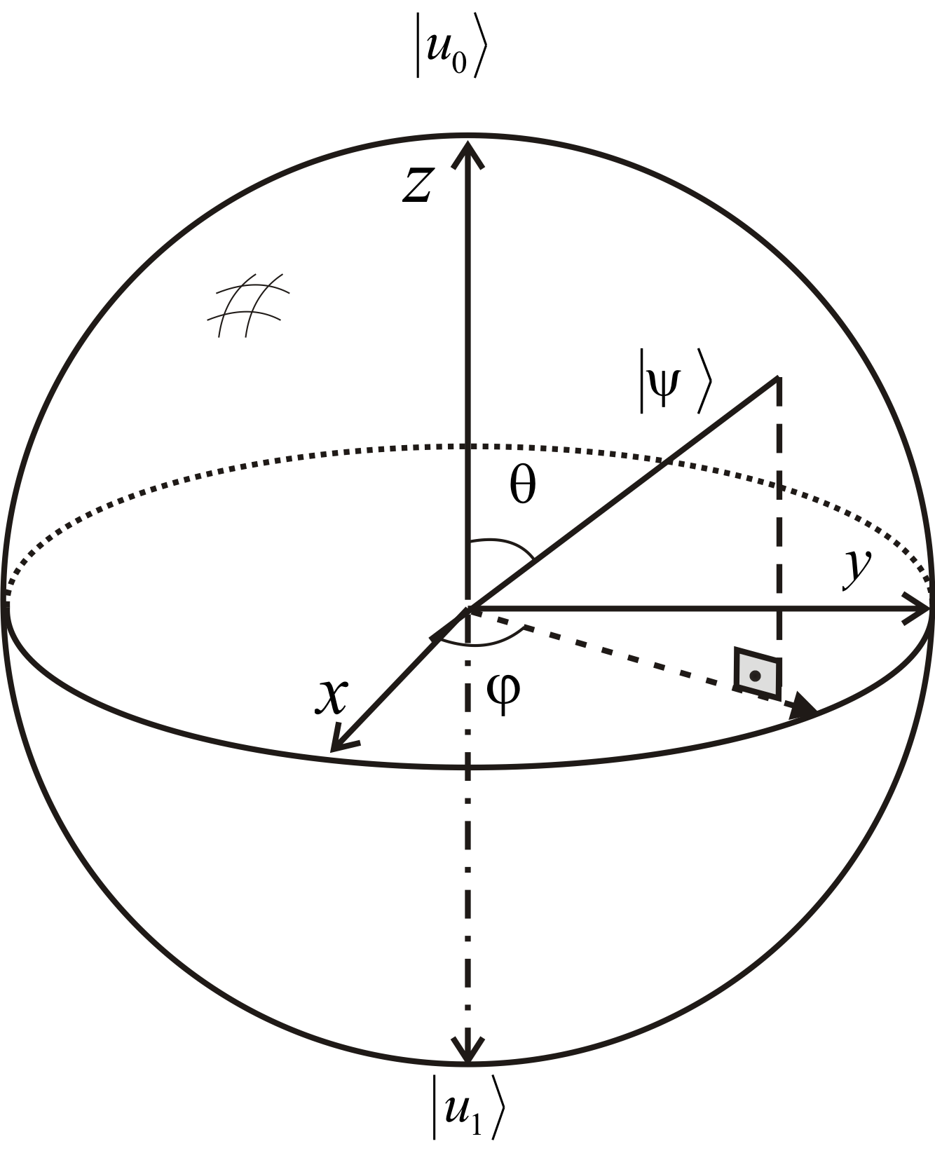
Figure 8: Bloch sphere

Let us introduce now a game between two parties, Alice and Bob. Alice chooses one of the two phases: $\alpha=0$ or $\alpha=\pi$ so that she has the following two states at her disposal:

$$\left|\pm\right\rangle=\frac{1}{\sqrt{2}}\left(\left|u_{0}\right\rangle\pm\left|u_{1}\right\rangle\right)$$ (107)

She delivers one of them to Bob and his task is to discover which one. All he has to do is to measure the $\hat{\sigma}_{1}$ observable:

$$\langle\hat{\sigma}_{1}\rangle_{\left|\pm\right\rangle}=\left\langle\pm\right|\hat{\sigma}_{1}\left|\pm\right\rangle=\pm 1$$ (108)

Thus, this is an example of a deterministic measurement because Bob has the previous knowledge that the state is an eigenstate of $\hat{\sigma}_{1}$ and so with one single measurement he discovers what was Alice’s choice and one classical bit has been transmitted between them. Suppose now that Alice chooses an arbitrary phase $\alpha$ and Bob must find out what is its value. In this case, Bob must measure a great number of equally prepared $\left|\psi_{\alpha}\right\rangle$ states so that he can find the average

$$\langle\hat{\sigma}_{1}\rangle_{\left|\psi_{\alpha}\right\rangle}=\left\langle\psi_{\alpha}\right|\hat{\sigma}_{1}\left|\psi_{\alpha}\right\rangle=\cos\alpha$$ (109)

After a sufficiently large number of measurements, he can find $\cos\alpha$. Since $\cos\alpha=\cos\left(2\pi-\alpha\right)$ there is still an ambiguity between these two possible states, but a few more measurements in the direction $\vec{\sigma}\cdot\hat{n}_{\alpha}$ where $\hat{n}_{\alpha}=\cos\alpha\hat{\imath}+\sin\alpha\hat{\jmath}$ solves the problem with ease. Thus, Bob can determine the phase $\alpha$ with arbitrary precision given a sufficiently large ensemble of equally prepared states $\left|\psi_{\alpha}\right\rangle$.

8.3 The Measurement of Interference for a Single Particle

Consider the quantum mechanic unidimensional motion of a single particle. Suppose that the particle in the instant $t=0$ is described as a sum of two highly concentrated “lumps” of the wave function at two macroscopically separated points. For instance, consider that at $t=0$, the single particle has just emerged from the interaction with a two-slit apparatus (with length $L$ between the slits). It is reasonable to expect that at this particular moment, the wave-function in the position basis is indeed highly localized around each one of the two slits. Let us consider the degree of freedom along the apparatus as the $y$ direction and the direction of the incident particle beam as the $x$-direction as shown in the figure 9.

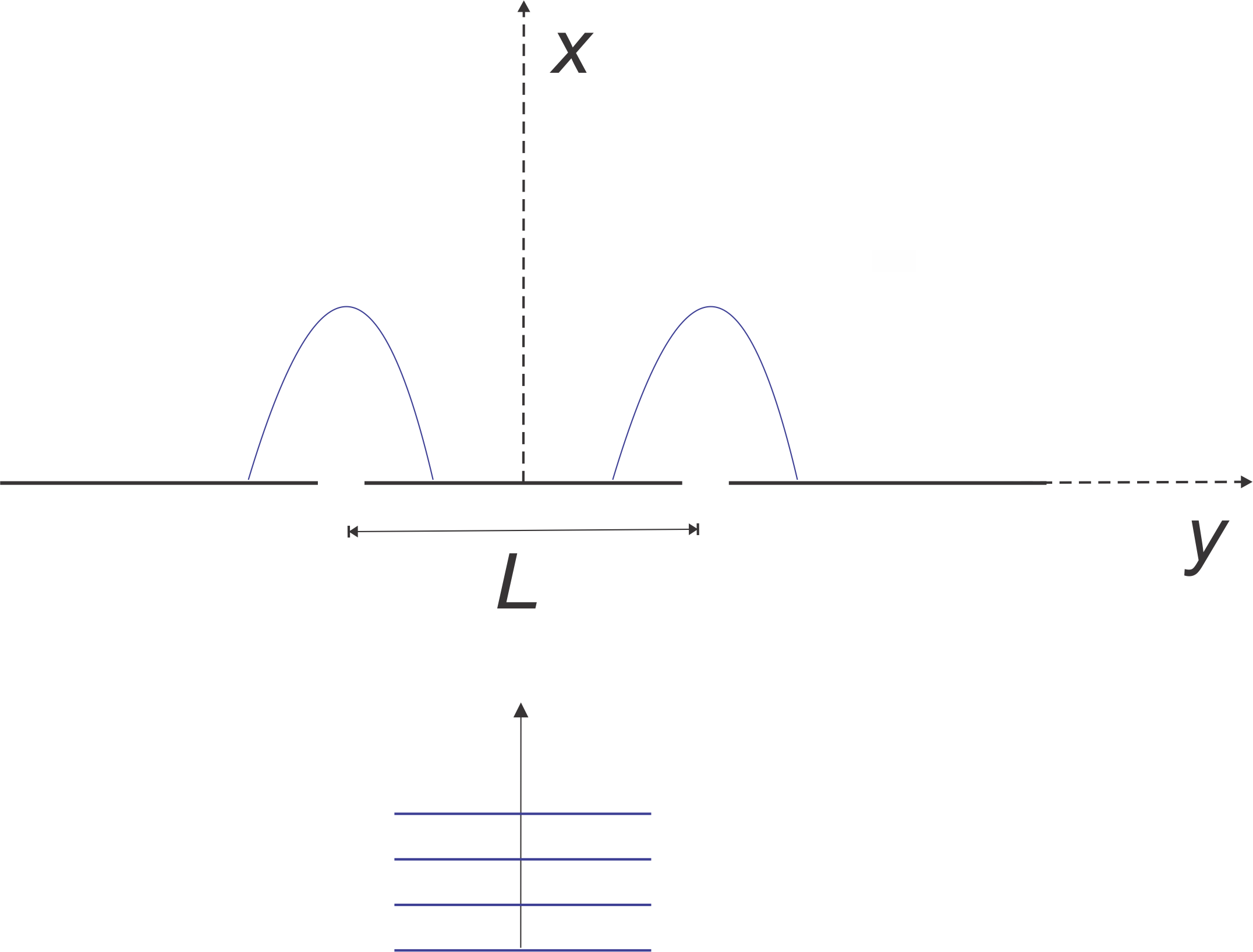
Figure 9: Two-Slit

Let the particle’s wave-function at $t=0$ be given by the following Schrödinger-Cat like state as a linear combination of two macroscopically separated coherent states (51)

$$\left|\varphi_{1}(0)\right\rangle=|p=0,q=-L/2\rangle\text{, and}$$

$$\left|\varphi_{2}(0)\right\rangle=|p=0,q=+L/2\rangle$$ (110)

where

$$|p,q\rangle=\hat{D}[p,q]|0\rangle=e^{-iqp/2}\hat{U}_{p}\hat{V}_{q}^{{\dagger}}|0\rangle$$ (111)

We are additionally supposing that the distance $L$ is much larger than the spread of the Gaussian wave functions (which in this case is given by $\delta=1/\sqrt{2}$) so that the overlap between $\left|\varphi_{1}(0)\right\rangle$ and $\left|\varphi_{2}(0)\right\rangle$ is negligible. Indeed, because of (52), we have that $\left|\left\langle\varphi_{2}(0)\right|\varphi_{1}(0)\rangle\right|^{2}=e^{-L^{2}/2}$. Suppose now that we take $L=10$, then
$|\langle\varphi_{2}(0)|\varphi_{1}(0)\rangle|^{2}\simeq 2\times 10^{-22}$ which implies that for all practical purposes the two states can indeed be considered orthogonal to each other. A general global normalized state of the particle can then approximately be written as the following linear combination

$$\left|\varphi_{\alpha}(0)\right\rangle\approx\frac{1}{\sqrt{2}}\left(|0,-L/2\rangle+e^{i\alpha}|0,+L/2\rangle\right)$$ (112)

Note that the above equation actually describes a family of states parametrized by the relative phase $\alpha$. The question here is the same that we asked in the previous subsection for the electron’s spin: How can we measure the relative phase? Note that no local measurements of the separate wave functions

$$\langle q(y)\left|\varphi_{1}(0)\right\rangle=\pi^{-1/4}e^{-\frac{1}{2}\left(y+L/2\right)^{2}}\text{, or}$$

$$\langle q(y)\left|\varphi_{1}(0)\right\rangle=\pi^{-1/4}e^{-\frac{1}{2}\left(y-L/2\right)^{2}}$$ (113)

can possibly detect the phase, since local phases are meaningless in quantum mechanics as only relative phases have any physical meaning and are measurable. Let us again initially allow Alice to choose between one of the following states (with $\alpha=0$ or $\alpha=\pi$) at $t=0$:

$$\left|\varphi_{\pm}(0)\right\rangle=\frac{1}{\sqrt{2}}\left(|0,-L/2\rangle\pm|0,+L/2\rangle\right)$$ (114)

The global wave-function in the position basis is then

$$\langle q(x)\left|\varphi_{\pm}(0)\right\rangle=\frac{\pi^{-1/4}}{\sqrt{2}}\left(e^{-\frac{1}{2}\left(x+L/2\right)^{2}}\pm e^{-\frac{1}{2}\left(x-L/2\right)^{2}}\right)$$ (115)

We have plotted in figure 10 the probability distributions $P_{\pm}(0)=\left|\langle q(x)\left|\varphi_{\pm}(0)\right\rangle\right|^{2}$ for both global states $\left|\varphi_{\pm}(0)\right\rangle$ at $t=0$ and for $L=10$.

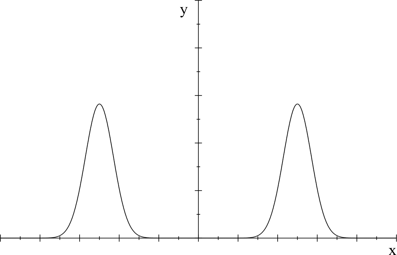
Figure 10: Initial Schrödinger-Cat state

To measure the relative phase, one would need to measure the whole global wave function non-locally. Each lump of the probability distribution would have to be measured locally (at $t=0$) and the information would have to be later compared. Yet, there is an easier method: one can “drive” both packets towards each other with a suitable Hamiltonian. Indeed, if we choose the Hamiltonian as (54) then the time evolution of a coherent state is trivial: Up to a phase, a coherent state remains a coherent state, imitating perfectly the motion in phase space of a classical harmonic oscillator. The best way to see this is through (53): The time evolution of each ket of the Shrödinger-cat superposition can now be easily computed as a dispersion-less rotation in phase space with unity frequency (up to an overall physically inessential phase):

$$\left|\varphi_{1}(t)\right\rangle =e^{-it\left(\hat{N}+\frac{1}{2}\hat{I}\right)}|0,-\frac{L}{2}\rangle=e^{-i\frac{t}{2}}|\frac{L}{2}\sin t,-\frac{L}{2}\cos t\rangle$$

$$\left|\varphi_{2}(t)\right\rangle =e^{-it\left(\hat{N}+\frac{1}{2}\hat{I}\right)}|0,\frac{L}{2}\rangle=e^{-i\frac{t}{2}}|-\frac{L}{2}\sin t,\frac{L}{2}\cos t\rangle$$ (116)

after a time $t=\pi/2$, both possible global state vectors are given by

$$\left|\varphi_{\pm}(\pi/2)\right\rangle=\frac{1}{\sqrt{2}}e^{-i\frac{\pi}{4}}\left(|+\frac{L}{2},0\rangle\pm|-\frac{L}{2},0\rangle\right)$$ (117)

where again $e^{-i\frac{\pi}{4}}$ is an unimportant overall phase factor. The motion in phase space is depicted in figure 11

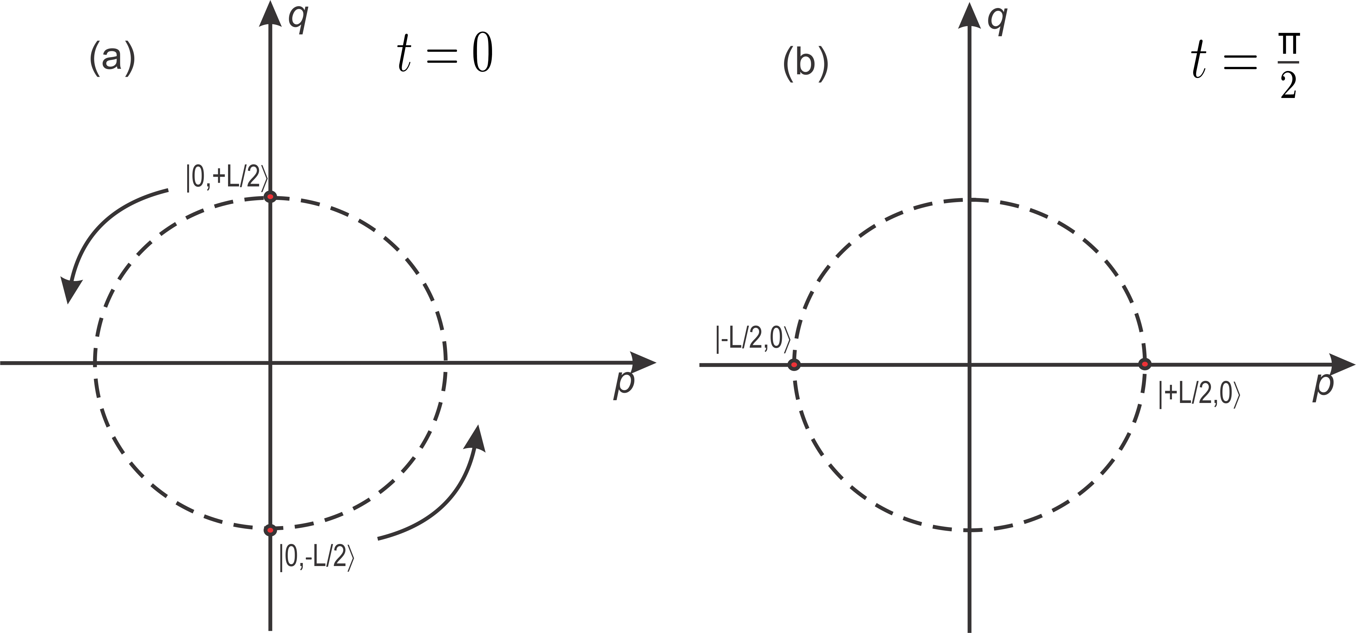
Figure 11: State evolution in Phase Space

In the position basis these state vectors can be written as

$$\langle q(x)\left|\varphi_{+}(\pi/2)\right\rangle=\sqrt{2}\pi^{-1/4}e^{-i\frac{\pi}{4}}\cos\left(\frac{Lx}{2}\right)e^{-\frac{1}{2}x^{2}}$$ (118)

and

$$\langle q(x)\left|\varphi_{-}(\pi/2)\right\rangle=\sqrt{2}i\pi^{-1/4}e^{-i\frac{\pi}{4}}\sin\left(\frac{Lx}{2}\right)e^{-\frac{1}{2}x^{2}}$$ (119)

We plot below the probability distribution $P_{+}(x)=\left|\langle q(x)\left|\varphi_{+}(\pi/2)\right\rangle\right|^{2}=\frac{2}{\sqrt{\pi}}\cos^{2}\left(5x\right)e^{-x^{2}}$ for $t=\pi/2$:

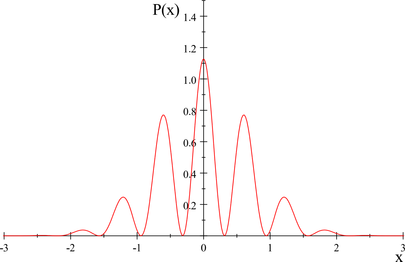
Figure 12: $P_{+}(x)$ for $t=\pi/2$ and $L=10$

We also plot below the probability distribution
$P_{-}(x)=\left|\langle q(x)\left|\varphi_{-}(\pi/2)\right\rangle\right|^{2}=\frac{2}{\sqrt{\pi}}\sin^{2}\left(5x\right)e^{-x^{2}}$ for $t=\pi/2$:

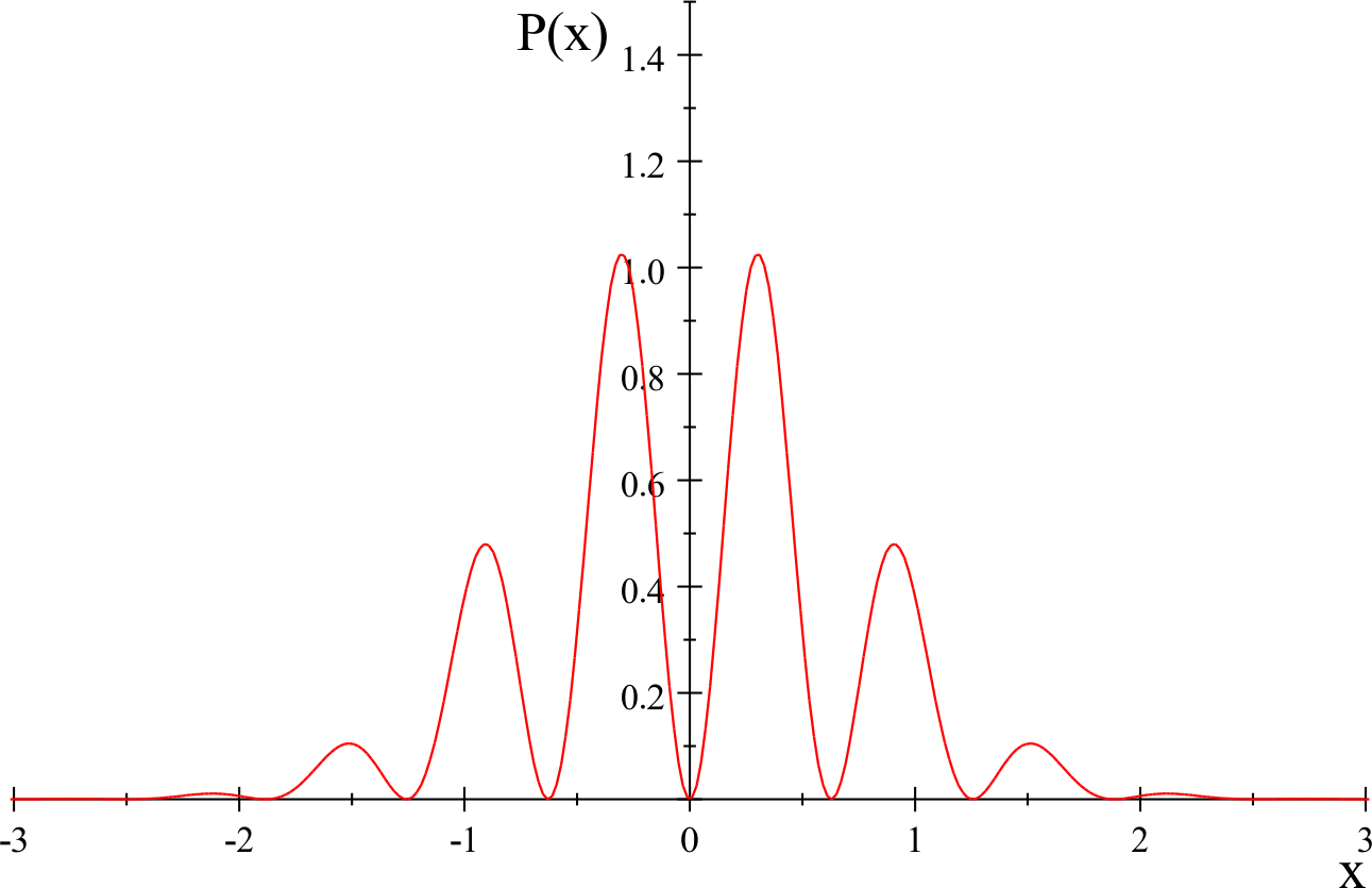
Figure 13: $P_{-}(x)$ for $t=\pi/2$ and $L=10$

Now that there is a superposition between the two pieces of wave-function, it is easy to see the interference pattern in both cases and so one could hope to distinguish them through local measurements. One possibility is to use the fact that the patterns are somewhat “complementary” in relation to each other in the sense that the maximum for the probability density for one pattern is the minimum for the other and vice-versa. For instance, suppose Bob sets up particle detectors at positions $x_{n}=n\pi/5$ (for $n=0,\pm 1,\pm 2,\pm 3$) at instant $t=\pi/2$ and where the precision of the detectors is given by $x_{n}\pm\Delta$ with $\Delta\approx 0.2$. One can estimate numerically that the probability of one of the detectors to “click” is about $93\%$ for state $\left|\varphi_{+}\right\rangle$ and $35\%$ for state $\left|\varphi_{-}\right\rangle$. This means that this method is unreliable for a single measurement to distinguish one state from the other. Bob would need to carry out a number of repetitions of this procedure for a set of equally prepared states by Alice in order to distinguish the states with confidence. For this reason and also because Bob has to perform a strong position measurement which will collapse the wave-function, we choose to coin this method as a partially deterministic measurement.

Suppose now that Alice prepares the cat state with an arbitrary phase $\alpha$ as in (112). After a time $t=\pi/2$, the state vector becomes

$$\left|\varphi_{\pm}(\pi/2)\right\rangle=\frac{1}{\sqrt{2}}e^{-i\frac{\pi}{4}}\left(|+\frac{L}{2},0\rangle\pm e^{i\alpha}|-\frac{L}{2},0\rangle\right)$$

$$=\frac{1}{\sqrt{2}}e^{-i\left(\frac{\pi-2\alpha}{4}\right)}\left(e^{-i\alpha/2}|+\frac{L}{2},0\rangle\pm e^{i\alpha/2}|-\frac{L}{2},0\rangle\right)$$ (120)

and the position basis wave-function can be written as

$$\langle q(x)\left|\varphi_{+}(\pi/2)\right\rangle=$$

$$=\sqrt{2}\pi^{-1/4}e^{-i\left(\frac{\pi-2\alpha}{4}\right)}\cos\left[\frac{1}{2}\left(Lx-\alpha\right)\right]e^{-x^{2}/2}$$ (121)

$$\langle q(x)\left|\varphi_{-}(\pi/2)\right\rangle=$$

$$=i\sqrt{2}\pi^{-1/4}e^{-i\left(\frac{\pi-2\alpha}{4}\right)}\sin\left[\frac{1}{2}\left(Lx-\alpha\right)\right]e^{-x^{2}/2}$$ (122)

If Alice provides Bob with a sufficiently large ensemble of equally prepared states, he can find the value of $\cos\alpha$ (or $\sin\alpha$) with arbitrary precision by measuring the particles position with a detector localized in $x=0$. Again we have a partially deterministic measurement of phase $\alpha$. It is important to note that, though one has in principle an infinite dimensional Hilbert space corresponding to the 1D motion of a quantum particle, since one is actually measuring a phase difference between two orthogonal states, in a sense one is effectively restrained to a two-level system (a qubit). Where can one actually find this qubit? The answer lies within the modular variable concept that we review in the next section.

9 Aharonov’s Modular Variables and Schwinger’s Formalism for Finite Quantum Mechanics

Though the space translation operator $\hat{V}_{L}=e^{i\hat{P}L}$ is not hermitean and therefore it is not a genuine quantum mechanical observable, one can consider the “phase” of such operator which is exactly the modular momentum. It is modular because it is clearly defined up to a value $p+\frac{2n\pi}{L}$ with $n\in Z$. Analogously, we can define a modular position variable as the phase of the momentum space translator $\hat{U}_{\frac{2\pi}{L}}=e^{\frac{2\pi i}{L}\hat{Q}}$ (with modular position given up to a value $q+nL$). It follows immediately from (11) that $\hat{V}_{L}$ and $\hat{U}_{\frac{2\pi}{L}}$ commute, so there are states that are simultaneously eigenkets both of modular momentum and modular position. For an apparatus formed by a lattice of a very large number $N$ of slits (with period $L$), one expects that $\phi(x)$ should be an $L$-periodic function and in this case, (1) implies that the modular momentum is exactly conserved. Consider the paradigmatic experiment of diffraction of a particle through such an apparatus with a large set of $N$ equidistant slits as in Figure 14.

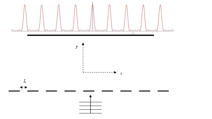
Figure 14: n-slit interference experiment.

One can model the interaction of the particle with the slits through the following Hamiltonian in the $x$ direction:

$$\hat{H}(t)=\frac{1}{2m}\hat{P}^{2}+V(\hat{Q})\delta(t)\text{, with}\quad V(\hat{Q}+L)=V(\hat{Q})$$ (123)

where the particle “hits the screen” at $t=0$. The fundamental physical assumptions here are that the interaction of the particle happens so fast that the unitary time evolution is given by $\hat{U}(t)\approx e^{-iV(\hat{Q})}$. By expanding this function in a Fourier series one gets

$$e^{-iV(\hat{Q})}=\sum\limits_{n\in Z}c_{n}e^{\frac{2\pi in}{L}\hat{Q}}=\sum\limits_{n\in Z}c_{n}\hat{U}_{\frac{2\pi n}{L}}$$ (124)

The initial state-vector (in the $x$ direction) of the particle is an eigenstate of momentum with zero momentum $\left|\psi_{(I)}\right\rangle=\left|p(0)\right\rangle$ so the state just after the interaction becomes $\left|\psi_{(F)}\right\rangle=\hat{U}(t)\left|p(0)\right\rangle$. The final state is then given by

$$|\psi_{(F)}\rangle=\sum\limits_{n\in Z}c_{n}\hat{U}_{\frac{2\pi n}{L}}\left|p(0)\right\rangle=\sum\limits_{n\in Z}c_{n}|p(\frac{2\pi n}{L})\rangle$$ (125)

The resulting state has indeed the remarkable property of being an eigenstate both of $\hat{U}_{2\pi/L}$ and $\hat{V}_{L}$. That $\left|\psi_{(F)}\right\rangle$ is indeed an eigenstate of $\hat{V}_{L}$ follows directly from (10). That the same state must also necessarily be an eigenstate of $\hat{U}_{2\pi/L}$ follows from the Weyl relation (11). Since $\hat{U}_{2\pi/L}$ and $\hat{V}_{L}$ commute and are also unitary, their eigenvalues are necessarily complex phases. This why Aharonov and collaborators coined these phases as modular variables. A phase space description of such a state is given by Figure 15.

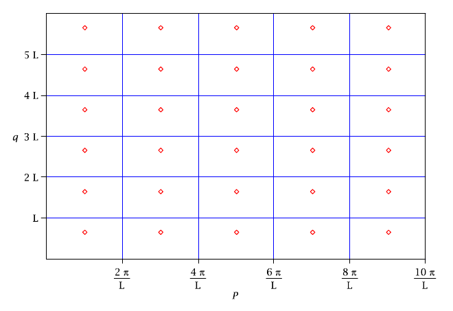
Figure 15: State with $q\ mod=2L/3$ and $pmod=\pi/L$.

This means that for the state represented above, one has that, in each cell, it is represented by an exact point with sharp values of modular position and momentum but there is a complete uncertainty about which cell it belongs to. This is a fundamental feature of the modular variable description. States with this peculiar mathematical structure have been also described by Zak to study systems with periodic symmetry in quantum mechanics zak1967 ; zak1968 . We may call them Aharonov-Zak states (AZ). Notice that the equation of motion (1) of the modular momentum is clearly non-local and one can perceive that this kind of “dynamical non-locality” can be naturally expressed within the Heisenberg picture. It would be almost impossible to capture this idea within the Schrödinger picture. Still one may address the question of how to describe explicitly the eigenkets of modular variables in a Schrödinger-like picture where one pays primary attention to the motion of the kets instead of the observables. The quantum vector space of the states of modular variables must be a finite-dimensional subspace (or at least a discrete subspace) of the infinite dimensional (continuous) space of states of the quantum motion of the particle in the $x$ direction. One possible approach to this description was given in aharonovpendletonpetersen which we briefly review below.

9.1 Aharonov´s Modular qubit

Consider the two-slit apparatus mentioned above. In this case, one should expect that the modular variables form a two-dimensional space (a spin $1/2$ algebra or a qubit algebra). One may define spin-like operators:

$$\hat{\sigma}_{3} =\frac{1}{2i}(\hat{U}_{\frac{\pi}{L}}-\hat{U}_{\frac{\pi}{L}}^{\dagger})$$ (126)

$$\hat{\sigma}_{1} =\frac{1}{2}(\hat{V}_{L}+\hat{V}_{L}^{\dagger})-\frac{1}{2}(\hat{V}_{L}-\hat{V}_{L}^{\dagger})\hat{\sigma}_{3}$$

$$\hat{\sigma}_{2} =-\frac{i}{2}(\hat{V}_{L}-\hat{V}_{L}^{\dagger})+\frac{i}{2}(\hat{V}_{L}+\hat{V}_{L}^{\dagger})\hat{\sigma}_{3}$$

acting upon a two-dimensional subspace of vectors given by $W^{(2)}=\left\{|q(+L/2)\rangle,|q(-L/2)\rangle\right\}$ from the infinite-dimensional (continuous) space $W^{(\infty)}=\left\{|q(x)\rangle,x\in\mathbb{R}\right\}$. By using (11) one can indeed check that the above operators obey the usual algebra for the Pauli matrices.

$$[\hat{\sigma}_{j},\hat{\sigma}_{k}]=2i\hat{\sigma}_{l}\varepsilon_{jk}^{l}\qquad\text{and\qquad}\left\{\hat{\sigma}_{j},\hat{\sigma}_{k}\right\}=2\hat{I}\delta_{jk}$$ (127)

when the operators defined in (126) are restricted to act upon $W^{(2)}$

$$\hat{\sigma}_{3}|q(\pm L/2)\rangle=\pm|q(\pm L/2)\rangle$$ (128)

so that the two sharp position eigenstates at each slit generate the modular qubit and they also diagonalize the $\hat{\sigma}_{3}$ operator. In this way, one can say that the full infinite-dimensional space $W^{(\infty)}$ is the direct sum $W^{(\infty)}=W^{(\infty\prime)}\oplus W^{(2)}$ of the Aharonov qubit $W^{(2)}$ with the (also infinite-dimensional space) $W^{(\infty\prime)}$=$\{|q(x)\rangle$, $x\in\mathbb{R}-\left\{\pm L/2\}\right\}$. We propose below a different approach to construct explicitly a qudit for modular variables based on Schwinger’s finite quantum kinematics.

9.2 The Schwinger-based Approach to the Modular Variable qubit

(The main references for this subsection are schwinger , schwinger1960 )

9.2.1 Schwinger’s Quantum Kinematics:

Let $W{\acute{}}^{(N)}$ be an $N$-dimensional quantum space generated by an orthonormal basis $\{\left|u_{k}\right\rangle\}$, $(k=0,1,\ldots N-1)$ which means that

$$|u_{k}\rangle\langle u^{k}|=\hat{I}\qquad\text{and}\qquad\langle u^{j}|u_{k}\rangle=\delta_{k}^{j}$$ (129)

These are considered to be finite position states. We also define a unitary translation operator $\hat{V}$ that acts cyclically over this basis:

$$\hat{V}\left|u_{k}\right\rangle=\left|u_{k-1}\right\rangle$$ (130)

The cyclicity implies that the following periodic boundary condition must be obeyed:

$$\left|u_{k+N}\right\rangle=\left|u_{k}\right\rangle$$

Which means that

$$\hat{V}^{N}=\hat{I}$$ (131)

so that the eigenvalues of $\hat{V}$ consists of the $N^{th}$ roots of unity:

$$\hat{V}\left|v_{k}\right\rangle=v_{k}\left|v_{k}\right\rangle\qquad\text{with}\qquad(v_{k})^{N}=1$$ (132)

The set $\{\left|v_{k}\right\rangle\},(k=0,1,2,\ldots N-1)$ is also an orthonormal basis of $W{\acute{}}^{(N)}$ (the finite set of momentum states) and the N distinct eigenvalues are explicitly given by

$$v_{k}=e^{\frac{2\pi i}{N}k}$$ (133)

With a convenient choice of phase, one can show that

$$\langle u^{j}|v_{k}\rangle=\frac{1}{\sqrt{N}}e^{\frac{2\pi i}{N}jk}=\frac{1}{\sqrt{N}}v_{k}^{j},$$

which is a finite analog of the plane wave function. It is not difficult to convince oneself of the following property:

$$\frac{1}{N}\sum\limits_{l=0}^{N-1}e^{\frac{2\pi i}{N}(j-k)l}=\delta_{jk}$$ (134)

One may then define a unitary translator $\hat{U}$ that acts cyclically upon the momentum basis analogously as was carried out for the $\hat{V}$ operator:

$$\hat{U}\left|v_{k}\right\rangle=\left|v_{k+1}\right\rangle$$

The same analysis applies now to the $\hat{U}$ operator and amazingly, the eigenstates of $\hat{U}$ can be shown to coincide with the original finite set of position basis with the same spectrum of $\hat{V}$:

$$\hat{U}\left|u_{k}\right\rangle=v_{k}\left|u_{k}\right\rangle$$

The finite index set $j,k=0,1,2,\ldots,N-1$ takes values in the finite ring $Z_{N}$ of $mod\ N$ integers. When $N=p$ is a prime number, $Z_{p}$ has the structure of a finite field. One distinguished property that is not difficult to derive is the well-known Weyl commutation relations between powers of the unitary translator operators which is a finite analog of (11).

$$\hat{V}^{j}\hat{U}^{k}=v^{jk}\hat{U}^{k}\hat{V}^{j}$$ (135)

In the next subsection, we carry out the continuous limit of Schwinger’s finite structure in order to present our proposal of a finite analogue of Aharonov’s modular variable concept and we also discuss the concept of pseudo-degrees of freedom lobonemes1995 , an idea that we believe to be essential in order to capture the true nature of the modular variables discrete Hilbert space.

9.3 Heuristic Continuum Limit

The implementation of the “continuum heuristic limit” (when the dimensionality of the quantum spaces approach infinity) can be performed in two distinct manners: one symmetric and the other non-symmetric between the position and momentum states. First, we briefly outline below, the symmetric case and following this, we present the non-symmetric limit which we shall use to discuss the modular variable concept.

9.3.1 The Symmetric Continuum Limit

Let the dimension $N$ of the quantum space be an odd number (with no loss of generality) and let us re-scale in equal footing the finite position and momentum states as

$$\left|q(x_{j})\right\rangle=\left(\frac{N}{2\pi}\right)^{1/4}\left|u_{j}\right\rangle\text{ and }\left|p(y_{k})\right\rangle=\left(\frac{N}{2\pi}\right)^{1/4}\left|v_{k}\right\rangle$$ (136)

with

$$x_{j}=\left(\frac{2\pi}{N}\right)^{1/2}j\qquad\text{and}\qquad y_{k}=\left(\frac{2\pi}{N}\right)^{1/2}k$$ (137)

so that the discrete indices are disposed symmetrically in relation to zero:

$$j,k=-\frac{(N-1)}{2},\ldots,+\frac{(N-1)}{2}\quad\text{ and}$$

$$\Delta x_{j}=\Delta y_{k}=\left(\frac{2\pi}{N}\right)^{1/2}$$ (138)

We may write the completeness relations for both basis as

$$\hat{I} =\sum\limits_{j=-\frac{(N-1)}{2}}^{+\frac{(N-1)}{2}}\left(\frac{2\pi}{N}\right)^{1/2}\left|q(x_{j})\right\rangle\left\langle q(x_{j})\right|$$

$$=\sum\limits_{k=-\frac{(N-1)}{2}}^{+\frac{(N-1)}{2}}\left(\frac{2\pi}{N}\right)^{1/2}\left|p(y_{k})\right\rangle\left\langle p(y_{k})\right|$$ (139)

One can give a natural heuristic interpretation of the $N\rightarrow\infty$ limit for the above equation as

$$\hat{I}=\int\limits_{-\infty}^{+\infty}dx\left|q(x)\right\rangle\left\langle q(x)\right|=\int\limits_{-\infty}^{+\infty}dy\left|p(y)\right\rangle\left\langle p(y))\right|$$ (140)

The generalized orthonormalization relations show that the new defined basis is formed by singular state-vectors with “infinite norm”:

$$\left\langle q(x_{j})\right|q(x_{k})\rangle =\left\langle p(x_{j})\right|p(x_{k})\rangle$$

$$=\underset{N\rightarrow\infty}{lim}\left(\frac{N}{2\pi}\right)^{1/2}\delta_{jk}\rightarrow\delta(x_{j}-x_{k})$$ (141)

The above equation also serves as a heuristic-based definition of the Dirac delta function as a continuous limit of the discrete Kronecker delta. Yet the overlap of elements from the distinct basis gives us the well-known plane-wave basis as expected:

$$\left\langle q(x_{j})\right|p(y_{k})\rangle=\frac{1}{\sqrt{2\pi}}e^{ix_{j}y_{k}}\qquad(\hbar=1)$$ (142)

9.3.2 The Non-Symmetric Continuum Limit

We introduce now a different scaling for the variables of position and momentum with a given $\xi\in\mathbb{R}$:

$$\left|q(x_{j})\right\rangle=\left(\frac{N}{\xi}\right)^{1/2}\left|u_{j}\right\rangle\text{ and }\left|p(y_{k})\right\rangle=\left(\frac{\xi}{2\pi}\right)^{1/2}\left|v_{k}\right\rangle$$ (143)

with

$$x_{j}=\frac{\xi}{N}j\qquad\text{and}\qquad y_{k}=\frac{2\pi}{\xi}k$$ (144)

so that

$$\Delta x_{j}=\frac{\xi}{N}\rightarrow 0\qquad\text{for}\qquad N\rightarrow\infty$$ (145)

Only the position states become singular and the $x_{j}$ variable takes value in a bounded quasi-continuum set so that the resolution of identity can be written as

$$\hat{I}_{\xi}=\int\limits_{-\xi/2}^{+\xi/2}dx\left|q(x)\right\rangle\left\langle q(x)\right|=\frac{2\pi}{\xi}\sum\limits_{k=-\infty}^{+\infty}\left|p(y_{k})\right\rangle\left\langle p(y_{k})\right|$$ (146)

Note that the momentum states continue to be of finite norm and their sum is taken over the enumerable but discrete set of integers $k\in Z$. The identity operator $\hat{I}_{\xi}$ can be thought as the projection operator on the subspace of periodic functions with period $\xi$. The overlap between position and momentum states is again given by the usual plane-wave function (142). Note also that we could have reversed the above procedure by choosing from the beginning the opposite scaling for the position and momentum states. In this case, the momentum eigenkets would form a continuous bounded set of singular state-vectors and the position eigenvectors would form an enumerable infinity of finite norm kets.

9.3.3 Pseudo Degrees of Freedom and the finite analog of the Aharonov-Zak states

In the $x^{1}-x^{2}$ plane, one can easily visualize the translations of the ket $\left|q(\vec{x})\right\rangle$ acted repeatedly upon with $\hat{V}_{\vec{\xi}}$ as in Figure 16, where the resulting position kets can be represented on a straight line in the plane that contains point $\vec{x}$ but with slope given by the $\vec{\xi}$ direction.

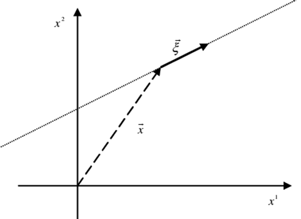
Figure 16: Two degrees of freedom.

Of course, to reach an arbitrary point in the plane, one needs at least two linear independent directions. This is precisely what one means when it is said that the plane is two-dimensional. But things for finite quantum spaces are not quite so simple. Let us consider first a 4-dimensional system given by the product of two 2-dimensional spaces (two qubits) $W^{(4)}=W^{(2)}\otimes W^{(2)}$ (it is important to notice here that one must not confuse the dimension of space, the so called degree of freedom with the dimensionality of the quantum vector spaces). We shall discard in the following discussion, the indices that indicate dimensionality to eliminate excessive notation. So let $\{\left|u_{0}\right\rangle,\left|u_{0}\right\rangle\}$ be the position basis for each individual qubit space so that computational (unentangled) basis of the tensor product spaces is $\{\left|u_{0}\right\rangle\otimes\left|u_{0}\right\rangle,\left|u_{0}\right\rangle\otimes\left|u_{1}\right\rangle,\left|u_{1}\right\rangle\otimes\left|u_{0}\right\rangle,\left|u_{1}\right\rangle\otimes\left|u_{1}\right\rangle\}$. One may represent such finite 2-space as the discrete set formed by the four points depicted in Figure 17:

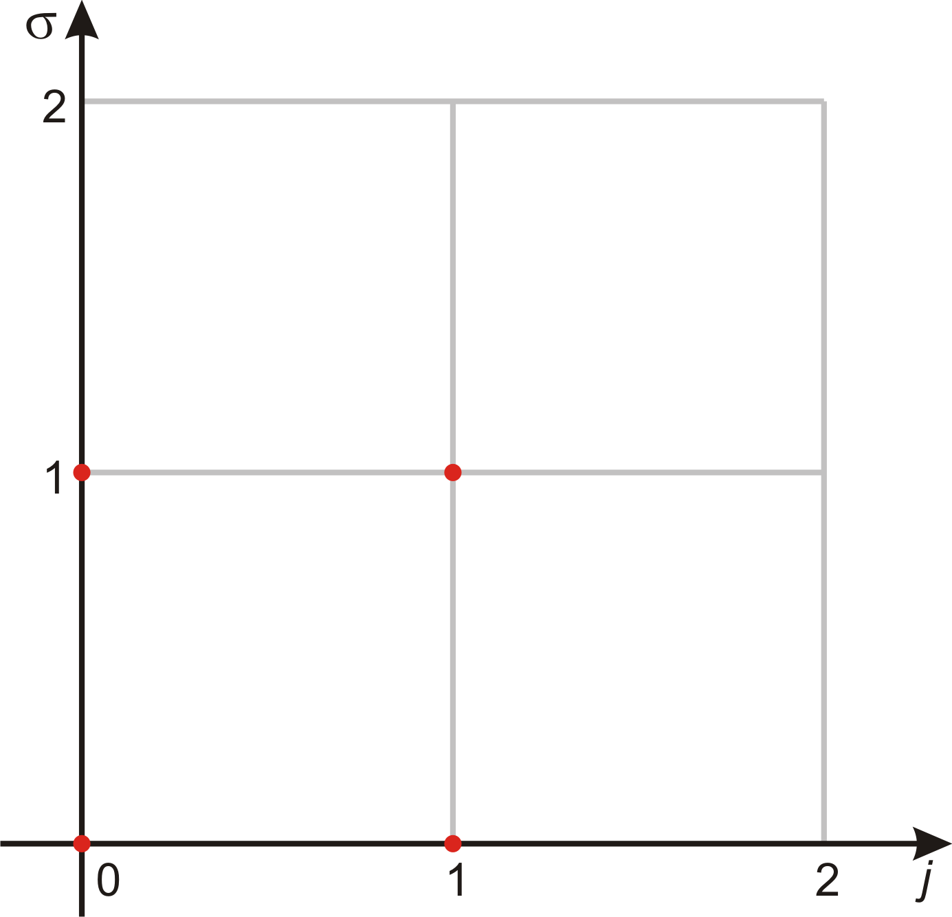
Figure 17: Finite 2-space for 2 qubits.

One may even construct distinct “straight lines” in this discrete two-dimensional space acting upon the computational basis $\{\left|u_{j}\right\rangle\otimes\left|u_{k}\right\rangle\}$ with the $\hat{V}\otimes\hat{V}$ operator as shown in Figure 18.

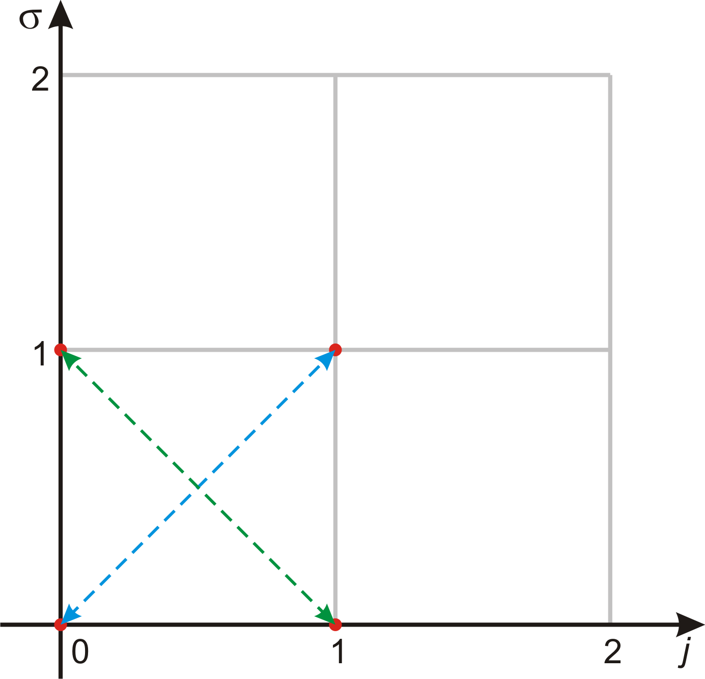
Figure 18: Discrete parallel lines (0, 0); (1, 1) and (0,1);(1,0).

Each of the two parallel “straight lines” are geometric invariants of the discrete 2-plane under the action of $\hat{V}\otimes\hat{V}$.

Consider now, a six-dimensional quantum space $W^{(6)}$ = $W^{(2)}\otimes W^{(3)}$ given by the product of a qubit and a qutrit with finite position basis given by respectively $\{\left|u_{0}\right\rangle,\left|u_{1}\right\rangle\}$ and $\{\left|u_{0}\right\rangle,\left|u_{1}\right\rangle,\left|u_{2}\right\rangle\}$. In this case, the fact the dimensions of the individual are coprime means that the action of the $\hat{V}\otimes\hat{V}$ operator on the product basis $\{\left|u_{j}\right\rangle\otimes\left|u_{\sigma}\right\rangle\},\ j=0,1$ and $\sigma=0,1,2$ can be identified with the action of $\hat{V}^{(6)}=\hat{V}^{(2)}\otimes\hat{V}^{(3)}$ on the same basis relabeled as $\{\left|u_{0}\right\rangle,\left|u_{1}\right\rangle,\left|u_{2}\right\rangle,\left|u_{3}\right\rangle,\left|u_{4}\right\rangle,\left|u_{5}\right\rangle\}$. One can start with the $\left|u_{0}\right\rangle\otimes\left|u_{0}\right\rangle$ state and cover the whole space with one single line as shown in Figure 19.

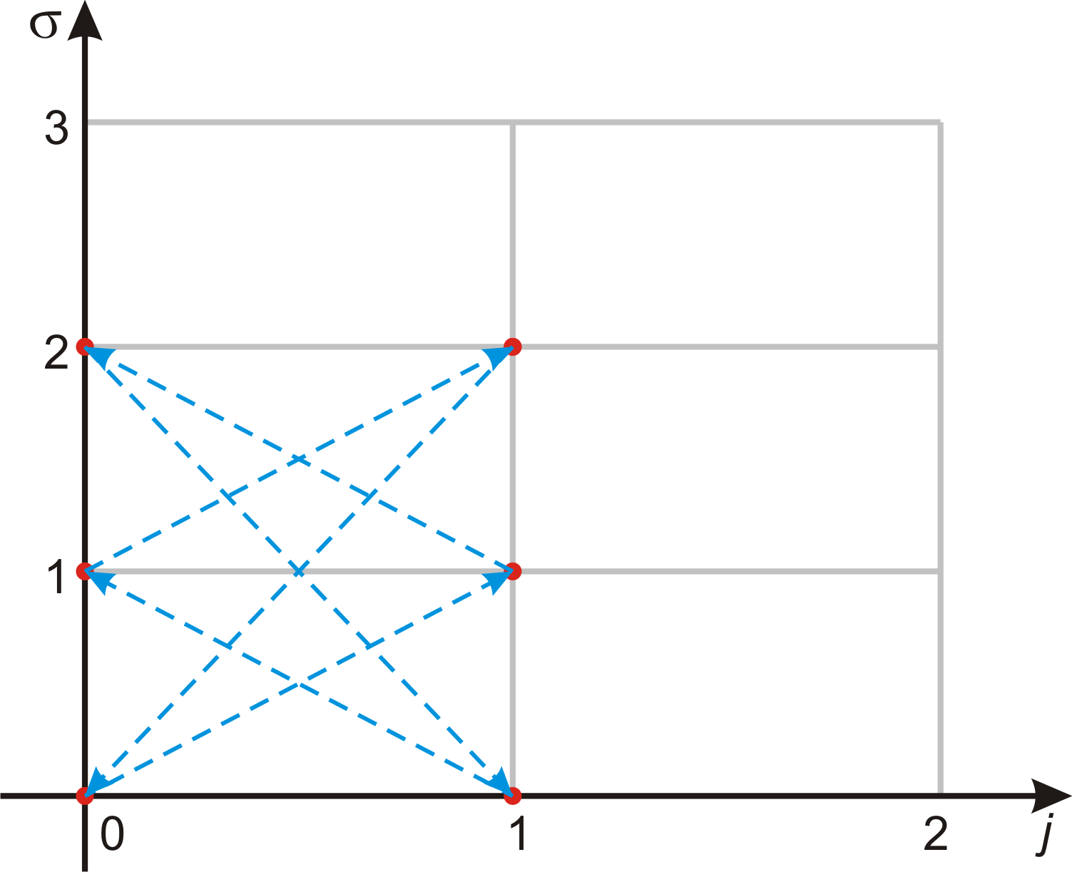
Figure 19: A single line covers the whole space.

This reduction of two degrees of freedom to only one single effective degree of freedom is a general fact for all product spaces when the dimensions of the factor spaces are co-prime. This fact follows from elementary number theory and it can be shown that when $gcd(N_{a},N_{b})=1$ for quantum spaces $W^{(N_{a})}$ and $W^{(N_{b})}$ then one may say that the two degrees of freedom are actually pseudo-degrees of freedom because one can associate only one effective single degree of freedom to the system in this sense. In the case above, it is easy to see that one of the pseudo degrees of freedom is nothing else but a factorizing period of the larger space. In this way we can either interpret the above finite six-dimensional position space as three periods of two or as two periods of three. All this is rather obvious and elementary, but surprisingly this is precisely the kind of mathematical structure that we propose to be behind Aharonov’s concept of modular variables. We can give a precise mathematical description of a finite analogue of this phenomenon in terms of the pseudo-degrees of freedom: consider $W^{(N)}=W^{(N_{a})}\otimes W^{(N_{b})}$ as the state space for a quantum mechanical system with $gcd(N_{a},N_{b})=1$. We can then offer an interpretation for this single degree of freedom of $W^{(N)}$ as a degree composed of “$N_{b}$ periods of size $N_{a}$” (or vice-versa). In fact, we may define the following state of $W^{(N)}$:

$$\left|j_{a},\sigma_{b}^{(N)}\right\rangle=\left|v_{j_{a}}{}^{(N_{a})}\right\rangle\otimes\left|u_{\sigma_{b}}{}^{(N_{b})}\right\rangle$$

This state is simultaneously an eigenstate of finite momentum of $W^{(N_{a})}$ and finite position of $W^{(N_{b})}$and clearly represents a finite analogue of the state represented in Figure 10. They are also simultaneous eigenstates of the (obviously commuting operators since they act on different spaces) unitary operators $\hat{V}^{(N_{a})}\otimes\hat{I}^{(N_{b})}$ and $\hat{I}^{(N_{a})}\otimes\hat{U}^{(N_{b})}$. Let us illustrate this again with an example of our “toy six-dimensional” case: Let the state $\left|1,2^{(6)}\right\rangle=\left|v_{1}{}^{(2)}\right\rangle\otimes\left|u_{2}{}^{(3)}\right\rangle$ be represented by the phase space plot (figure 20).

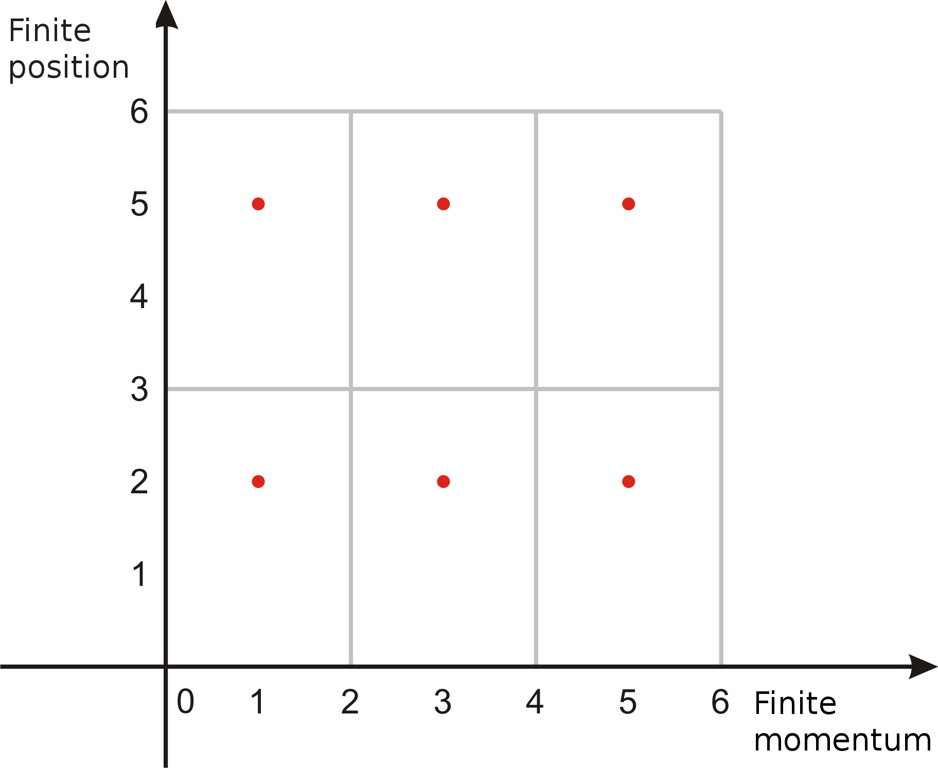
Figure 20: State $\left|1,2^{(6)}\right\rangle\in W^{\left(6\right)}$.

States with this peculiar mathematical structure have been also described by Zak to study systems with periodic symmetry in Quantum Mechanics zak1967 ; zak1968 . We may call them Aharonov-Zak states (AZ). The particular AZ state obtained in the $n$-slit (with large enough $n$) can be thought as obtained by an ideal projective measurement performed by the slit apparatus on the second modular variable subspace of the particle:

$$|v_{0}^{(N_{a})}\rangle\otimes|v_{0}^{(N_{b})}\rangle\overset{projective``space"measurement}{\underset{in\ the\ \sec ond\ subspace}{\Longrightarrow}}$$

$$|v_{0}^{(N_{a})}\rangle\otimes|u_{0}^{(N_{b})}\rangle=\frac{1}{\sqrt{N_{b}}}\sum\limits_{\sigma_{b}=0}^{N_{b}-1}|v_{0}^{(N_{a})}\rangle\otimes|v_{\sigma_{b}}^{(N_{b})}\rangle$$ (147)

The continuum limit of the AZ state can be constructed through the non-symmetric limit discussed in a previous subsection. The only care that must be taken is that, given the two subspaces, the opposite limit must be taken for each subspace. That is, if one chooses to make the momentum basis of the first subspace go to infinity as a bounded continuum, then for the second subspace it is the position basis that must become a bounded continuum set and vice-versa.

10 Concluding Remarks

We presented a compact review of some phase-space formalisms of quantum mechanics, with also a more intrinsic and coordinate independent notation, in order to discuss some of its most outstanding and up-to-date applications: namely the theory of modular variables and the concept of weak values developed by Yakir Aharonov and his many collaborators in the last forty years. The theory of non-relativistic Quantum Mechanics was created, or discovered, back in the 1920’s mainly by Heisenberg and Schrödinger, but it is fair enough to say that a more modern and unified approach to the subject was introduced by Dirac and Jordan with their (intrinsic) Transformation Theory. In his famous text book on Quantum Mechanics Dirac , Dirac introduced his well-known bra and ket notation and a view that even Einstein, who was, as is well known, very critical towards the general quantum physical world-view, considered the most elegant presentation of the theory at that time Farmelo . One characteristic of this formulation is that the observables of position and momentum are truly treated equally so that an intrinsic phase-space approach seems a natural course to be taken. In fact, we may distinguish at least two different quantum mechanical approaches to the structure of the quantum phase space: The Weyl-Wigner formalism and the advent of the theory of coherent states. We have used these phase-space formalisms of Quantum Mechanics in order to describe two major insights due to Aharonov and his many collaborators over the last four decades: The concept of weak values and those of modular variables. The quantum mechanical phase space approach is particularly well suited to decribe the concept of weak value as complex number-valued element of reality where both the real and imaginary parts have equal physical status in the theory. The modular variable is a concept that is slightly more difficult to grasp mathematically. It gives rise to dynamical non-local effects which seem to be intrinsically different from the kinematic non-local effects of entangled states like EPR pairs of particles.

Though there is no doubts about the fact that the structure of modular variables is much easier to understand intuitively within the Heisenberg picture, the problem of how to describe the finite dimensional Hilbert space where the modular variables actually “live in” is a quite different and subtle issue. It is very important to notice that the Schwinger-like approach that we present here for the construction of the modular variable qubits (or qudits) is different from the original path chosen by Aharonov and collaborators. In their original approach, the whole state space is a direct sum between the modular variable qudit space and the “rest of the quantum space” while in the Schwinger-based approach the whole state space is the tensor product between the qudit space and “the rest of the quantum space”. This difference is not just one of academic nature. One must remember the important fact that the rule of how one compounds two distinct quantum systems is described mathematically by the tensor product between each subsystem instead of their direct sum. This important fact is what is behind one of the most fundamental differences between classical and quantum physics, the phenomenon of quantum entanglement which is the basis of modern quantum information theory. One may speculate that this fact could lead to some possible experimental procedure in order to decide this important issue. One could envisage the use of the quantum mechanical “pseudo-degrees of freedom” (as the periodicity of a lattice of slits) as a new resource for manipulation and storage of qubits with possible new applications in the field of quantum information. We also hope that this may help to shed some light on the physical differences between dynamic non-locality and that of kinematic non-locality in quantum physics.

- (1) Y. Aharonov, D. Bohm, Phys. Rev. 115(3), 485 (1959). DOI 10.1103/PhysRev.115.485
- (2) Y. Aharonov, H. Pendleton, A. Petersen, International Journal of Theoretical Physics 2(3), 213 (1969)
- (3) Y. Aharonov, D. Rohrlich, Quantum Paradoxes: Quantum Theory for the Perplexed (Wiley, 2003)
- (4) Y. Aharonov, arXiv preprint arXiv:1303.2137 (2013)
- (5) Y. Aharonov, P.G. Bergmann, J.L. Lebowitz, Physical Review 134(6B), B1410 (1964)
- (6) Y. Aharonov, D.Z. Albert, L. Vaidman, Physical review letters 60(14), 1351 (1988)
- (7) Y. Aharonov, A. Botero, S. Popescu, B. Reznik, J. Tollaksen, Physics Letters A 301(3), 130 (2002)
- (8) P.B. Dixon, D.J. Starling, A.N. Jordan, J.C. Howell, Phys. Rev. Lett. 102(17), 173601 (2009). DOI 10.1103/PhysRevLett.102.173601
- (9) O. Hosten, P. Kwiat, Science 319(5864), 787 (2008)
- (10) M. Berry, P. Shukla, Journal of Physics A: Mathematical and Theoretical 43(35), 354024 (2010)
- (11) V.I. Arnol’d, Mathematical methods of classical mechanics (Springer, 1989)
- (12) R. Abraham, J.E. Marsden, T.S. Rațiu, R. Cushman, Foundations of mechanics (Benjamin/Cummings Publishing Company Reading, Massachusetts, 1978)
- (13) J.R. Klauder, E.C.G. Sudarshan, Fundamentals of quantum optics (Courier Dover Publications, 2006)
- (14) S.R. De Groot, L.G. Suttorp, Foundations of electrodynamics (North-Holland Publishing Company, 1972)
- (15) J.J. Sakurai, Modern Quantum Mechanics (Addison Wesley, 1994)
- (16) A. Böhm, M. Gadella, J.D. Dollard, Dirac Kets, Gamow Vectors, and Gel’fand Triplets: The Rigged Hilbert Space Formulation of Quantum Mechanics: Lectures in Mathematical Physics at the University of Texas at Austin (Springer-Verlag, 1989)
- (17) J. Schwinger, Quantum kinematics and dynamics (Westview Press, 2000)
- (18) D. Page, Physical Review A 36(7), 3479 (1987)
- (19) J. Anandan, Y. Aharonov, Phys. Rev. Lett. 65, 1697 (1990). DOI 10.1103/PhysRevLett.65.1697
- (20) W.M. Zhang, R. Gilmore, et al., Reviews of Modern Physics 62(4), 867 (1990)
- (21) A. Perelomov, Generalized coherent states and their applications (Springer-Verlag New York Inc., New York, NY, 1986)
- (22) J.R. Klauder, B.S. Skagerstam, Coherent states: applications in physics and mathematical physics (World scientific, 1985)
- (23) M. Combescure, D. Robert, Coherent states and applications in Mathematical Physics (Springer, 2012)
- (24) V. Namias, IMA Journal of Applied Mathematics 25(3), 241 (1980)
- (25) V. Vedral, Modern foundations of quantum optics (Imperial College Press, 2005)
- (26) Y. Aharonov, L. Vaidman, in Time in Quantum Mechanics (Springer, 2007), pp. 399–447
- (27) J. von Neumann, Mathematical Foundations of Quantum Mechanics (Princeton University Press, 1996)
- (28) R. Jozsa, Phys. Rev. A 76(4), 044103 (2007). DOI 10.1103/PhysRevA.76.044103
- (29) S. Tamate, H. Kobayashi, T. Nakanishi, K. Sugiyama, M. Kitano, New Journal of Physics 11, 093025 (2009)
- (30) S. Pancharatnam, Proc. Indian Acad. Sci. A 44, 247 (1956)
- (31) M. Berry, Proceedings of the Royal Society of London. Series A, Mathematical and Physical Sciences 392(1802), 45 (1984)
- (32) Y. Aharonov, J. Anandan, Physical Review Letters 58(16), 1593 (1987)
- (33) H. Kobayashi, K. Nonaka, Y. Shikano, arXiv preprint arXiv:1311.3357 (2013)
- (34) A.C. Lobo, R.A. Ribeiro, C. de Assis Ribeiro, P.R. Dieguez, European Journal of Physics 33(5), 1063 (2012)
- (35) Y. Shikano, in Measurements in Quantum Mechanics, ed. by J.R. Pahlavani (InTech, InTech, 2012). URL http://www.intechopen.com/books/measurements-in-quantum-mechanics/theory-of-weak-value-and-quantum-mechanical-measurement
- (36) J. Dressel, M. Malik, F.M. Miatto, A.N. Jordan, R.W. Boyd, Rev. Mod. Phys. 86, 307 (2014). DOI 10.1103/RevModPhys.86.307. URL http://link.aps.org/doi/10.1103/RevModPhys.86.307
- (37) J. Tollaksen, in Proc of SPIE Vol. 6573 (SPIE, Bellingham, WA), CID 6573-33, ed. by E. Donkor, A. Pirich, H. Brandt (2007)
- (38) J. Zak, Physical Review Letters 19, 1385 (1967)
- (39) J. Zak, Physical Review 168(3), 686 (1968)
- (40) J. Schwinger, Proceedings of the national academy of sciences of the United States Of America 46(4), 570 (1960)
- (41) A.C. Lobo, M. Nemes, Physica A: Statistical Mechanics and its Applications 216(1), 185 (1995)
- (42) P.A.M. Dirac, The principles of quantum mechanics (The International Series of Monographs on Physics, Oxford University Press, 1947)
- (43) G. Farmelo, The strangest man: the hidden life of Paul Dirac, quantum genius (Faber & Faber, 2009)