Time-dependent potential barriers and superarrivals

Abstract

Scattering of a Gaussian wavepacket from rectangular potential barriers with increasing widths or heights is studied numerically. It is seen that during a certain time interval the time-evolving transmission probability increases compared to the corresponding unperturbed cases. In the literature this effect is known as superarrival in transmission probability. We present a trajectory-based explanation for this effect by using the concept of quantum potential energy and computing a selection of Bohmian trajectories. Relevant parameters in superarrivals are determined for the case that the barrier width increases linearly during the dispersion of the wavepacket. Nonlinear in time perturbation is also considered.

I Introduction

Success in numerical solution of time-dependent differential equations in recent decades has provided a powerful tool for studying quantum systems with time-dependent boundary. Interesting phenomena like diffraction in time Mo-PR-1952 and superarrivals BaMaHo-PRA-2002 ; MaHo-Pranama-2002 ; MaMaHoPLA-2002 ; HoMaMa-JPA-2012 are seen in such systems with time-dependent Hamiltonians. Superarrivals is observed when a rectangular potential barrier is perturbed by changing its height during the scattering of a Gaussian wavepacket in a very short time: compared to the unperturbed situation an enhancement in the time-dependent transmission (reflection) probability is seen for a specific time-interval if the barrier height is raised (reduced) BaMaHo-PRA-2002 ; MaHo-Pranama-2002 ; MaMaHoPLA-2002 . This phenomenon has been explained by taking the Schrödinger wavefunction as a real physical field: disturbance due to the perturbed barrier propagates through this field to the measuring apparatus. Propagation speed depends on the rate of change in barrier height BaMaHo-PRA-2002 ; MaHo-Pranama-2002 ; MaMaHoPLA-2002 . The origin of superarrivals has been explained by the concept of quantum potential energy MaMaHoPLA-2002 in Bohmian mechanics. Recently superarrivals were studied for a parabolic potential barrier in position with a time-dependent intensity and it was shown that this effect can be interpreted semiclassically HoMaMa-JPA-2012 . It was argued that this phenomenon can be used in secure transmission of information MaHo-Pranama-2002 ; HoMaMa-JPA-2012 .

We aim to consider superarrivals in some more general situations. We will proceed as follows: The occurrence of superarrivals is shown in section II for the scattering of a Gaussian wavepacket by a rectangular barrier whose width increases linearly in time. Then we study the effect of perturbation on the time-evolving expectation values of Hamiltonian, momentum and position operators for the transmitted part of the wavepacket. After, superarrivals are studied in the context of Bohm’s causal theory by computing a selection of Bohmian trajectories and noting the concept of quantum potential energy. Section III generalizes the problem to the case where the height of the potential barrier increases nonlinearly from zero to a finite height. Finally, a summary of our conclusions will be presented in section IV.

II Gaussian wavepacket and linear increase in barrier width

Consider an ensemble of single-particle scattering experiments. In each trial, a particle described by a Gaussian wavepacket $\psi_{0}(x)$

$$\psi_{0}(x)=\frac{1}{(2\pi\sigma_{0}^{2})^{1/4}}~{}e^{-(x-x_{0})^{2}/4\sigma_{0}^{2}+ip_{0}(x-x_{0})/\hbar}~{},$$ (1)

is incident at $t=0$ from the left on a potential barrier of height $V_{0}$. At a point $x_{d}$ in the right of the barrier is an ideal detector that triggers when the particle reaches the plane $x=x_{d}$. The initial centroid $x_{0}$ and root mean square width $\sigma_{0}$ of $\psi_{0}(x)$ is chosen in a way that it has a negligible overlap with the potential barrier. Then, the time-varying transmission probability is given by

$$T(t) = \int_{x_{d}}^{\infty}|\psi\left(x,t\right)|^{2}dx~{}.$$ (2)

The above study is done for both the case of a static barrier, $V(x)=V_{0}~{}\theta(x)~{}\theta(w_{i}-x)$, and also when the barrier is perturbed by increasing its width from the initial width $w_{i}$ to a final width $w_{f}$ linearly in time, $V(x,t)=V_{0}~{}\theta(x)~{}\theta(w(t)-x)$. Here, $\theta(x)$ is the step function and $w(t)$ is the time-dependent width of the perturbed barrier,

$$w(t) = \begin{cases}w_{i}&\text{if }t\leq t_{p}\\ w_{i}+\dfrac{w_{f}-w_{i}}{\varepsilon}(t-t_{p})&\text{if}~{}t_{p}<t\leq t_{p}+\varepsilon\\ w_{f}&\text{if }t>t_{p}+\varepsilon\end{cases}~{},$$

where $t_{p}$ is the time at which perturbation is started and $\varepsilon$ is the duration of perturbation.

We compute $\psi(x,t)$ in whole space at any instant by using the Crank-Nikolson method for numerical solution of the time-dependent Schrödinger equation. In this regard $[0,40t_{0}]$ ($t_{0}=m\sigma_{0}/p_{0}$) is taken as time range and $[-500\sigma_{0},500\sigma_{0}]$ as space range. For numerical calculations we work in a system of units where $\hbar=1$ and $m=1/2$ and parameters are chosen in a way that spreading of the packet is negligible during the scattering process. The constants are chosen as follows: $\sigma_{0}=\sigma_{1}/\sqrt{2}$, $x_{0}=-6\sigma_{1}$, $p_{0}=50\pi$, $V_{0}=1.5E_{0}$, $w_{i}=0.08\sigma_{1}$ , $w_{f}=0.48\sigma_{1}$ and $x_{d}=10\sigma_{1}$ where $\sigma_{1}=0.05$. Here, $E_{0}=p_{0}^{2}/2m+\hbar^{2}/8m\sigma_{0}^{2}$ is the expectation value of energy for the initial packet. Fig. 1 shows time-varying transmission probability $T(t)$ for both static and perturbed barriers. Here, perturbation takes place in time interval $[7.14t_{0},7.41t_{0}]$, that is $\varepsilon=0.27t_{0}$. Noting this figure one finds a finite time interval $\Delta t$ during which the probability of transmission in the perturbed case is greater than the corresponding value for the unperturbed case (superarrivals in transmission probability). This means in the perturbed case it is possible to find the particle beyond the detector after a shorter time, although the overall probability of finding the particle beyond the detector is much suppressed; $\lim_{t\rightarrow\infty}T_{s}(t)\simeq 0.79$ while $\lim_{t\rightarrow\infty}T_{p}(t)\simeq 0.11$. Here and in the following the subscript ”$s$” (”$p$”) stands for the static (perturbed) situation. Following BaMaHo-PRA-2002 we show the time interval of early arrivals by $\Delta t=t_{c}-t_{d}$ where $t_{c}$ is the instant when the two curves cross and $t_{d}$ is the time when their deviation starts. From figure 1 one finds $t_{d}\simeq 10.41t_{0}$ and $t_{c}\simeq 20.29t_{0}$.

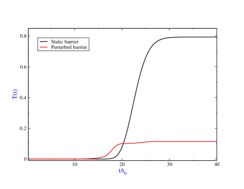
Figure 1: (Color online) Time-evolving transmission probability during the scattering of a Gaussian packet by a barrier with a constant (black curve) and a width in linear increase (red curve).

To see the origin of these early arrivals we examine mean value of observables. Expectation value of an observable $\hat{A}$ with respect to the transmitting part of the packet is given by

$$\langle\hat{A}\rangle_{\text{T}}(t) = \frac{\int_{x_{d}}^{\infty}\psi^{*}(x,t)~{}A(x)~{}\psi(x,t)dx}{T(t)}~{},$$

where subscript ”T” stands for transmission and $A(x)$ is the observable $\hat{A}$ in the position representation. Due to a kick imparted by the perturbed barrier, transmitted packet moves faster in the perturbed situation in comparison to the unperturbed case. As a result the mean energy and momentum of transmitted packet for the perturbed barrier exceeds those for the static case. See Fig. 2. This leads to the sooner arrival of the particles at the detector place. Deviation of perturbed and static curves takes place at $t_{d}$ in agreement with that of Fig. 1. Asymptotic values of $\langle\hat{H}\rangle_{T}$ and $\langle\hat{p}\rangle_{T}$ are respectively $1.92E_{0}$ and $1.34p_{0}$ for the perturbed situation. In this limit $\langle\hat{x}\rangle_{T}$ moves with a constant velocity.

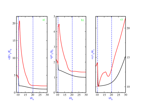
Figure 2: (Color online) Expectation value of (a) Hamiltonian, (b) momentum and (c) position with respect to the transmitting wavepacket. In all plots black curve shows the static situation while the red one stands for the perturbed barrier. Vertical blue dashed lines show $t_{d}$ and $t_{c}$.

As a measure of early arrivals the quantity

$$\eta = \dfrac{I_{p}-I_{s}}{I_{s}}~{},$$ (3)

has been defined BaMaHo-PRA-2002 , where $I_{p}$ and $I_{s}$ are respectively the area under the curves of $T_{p}(t)$ and $T_{s}(t)$ during the time interval $\Delta t$:

$$I_{p} = \int_{\Delta t}T_{p}(t)dt~{},~{}~{}~{}~{}~{}~{}~{}~{}I_{s}=\int_{\Delta t}T_{s}(t)dt~{}.$$ (4)

The magnitude $\eta$ of superarrivals has been plotted for three different values of barrier height $V_{0}$ versus the duration of perturbation $\varepsilon$ in figure 3a).

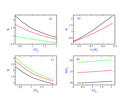
Figure 3: (Color online) a) Superarrivality $\eta$ versus duration of perturbation $\varepsilon$ for three different values of barrier height: $V_{0}=E_{0}$ (green curve), $V_{0}=1.3E_{0}$ (red curve) and $V_{0}=1.5E_{0}$ (black curve). b) Superarrivality $\eta$ versus final width $w_{f}$ of the barrier for two different values of duration of perturbation: $\varepsilon=0.27t_{0}$ (black curve) and $\varepsilon=0.80t_{0}$ (red curve). c) Superarrivality $\eta$ versus duration of perturbation $\varepsilon$ for three different values of detector location: $x_{d}=10\sigma_{1}$ (black curve) and $x_{d}=15\sigma_{1}$ (red curve) and $x_{d}=20\sigma_{1}$ (green curve). d) Duration of superarrivals $\Delta t$ versus duration of perturbation $\varepsilon$ for three different detector location: $x_{d}=10\sigma_{1}$ (black curve) and $x_{d}=15\sigma_{1}$ (red curve) and $x_{d}=20\sigma_{1}$ (green curve).

One sees that $\eta$ decreases with $\varepsilon$ for a given value of $V_{0}$ while for a given value of duration of perturbation, superarrivality increases with the height of the barrier. In Fig. 3b) we have plotted $\eta$ versus $w_{f}$ for two different values of $\varepsilon$. One sees that the magnitude of superarrivals increases with the final width of the perturbed barrier. In figures 3c) and 3d) we have plotted $\eta$ and $\Delta t$ versus $\varepsilon$ for three different values of detector position. According to these plots we can say that for a given value of $\varepsilon$, magnitude and duration of superarrivals increase when the distance of the detector from the barrier becomes larger. Increment of $\Delta t$ with $\varepsilon$ is gradual for a given value of $x_{d}$.

Our aim is now description of early arrivals within the framework of Bohmian mechanics (BM). In BM complete description of a system is given by its wavefunction and position. The wavefunction which is the solution of the Schrödinger equation guides the particle motion by the guidance equation,

$$\dot{x}(t) = \frac{1}{m}\nabla S(x,t)\bigg{|}_{x=x(t)}~{},$$ (5)

where, $S$ is the phase of the wavefunction in its polar form $\psi=Re^{iS/\hbar}$ and $x(t)$ is the particle trajectory Ho-Book-1993 . BM reproduces the results of the standard quantum mechanics provided that distribution of initial positions is given by $\rho=|\psi|^{2}$. Particle trajectories are obtained by integrating the guidance equation (5) for a given initial position $x^{(0)}$. In the second-order point of view of BM acceleration of Bohmian particle along its trajectory is given by

$$\ddot{x} = -\frac{1}{m}\nabla(V+Q)\bigg{|}_{x=x(t)}~{},$$

where the particle is subjected to a quantum force $-\nabla Q$ in addition to the classical force $-\nabla V$ Ho-Book-1993 . $Q$ is called quantum potential and is given by

$$Q(x,t) = -\dfrac{\hbar^{2}}{2m}\frac{\nabla^{2}R}{R}~{},$$

where R is the amplitude of the wavefunction. Due to the non-crossing property of Bohmian trajectories, there is a critical trajectory (starting at $x_{c}^{(0)}$) that separates transmitted trajectories from the reflected ones in a scattering process and is given by Le-PLA-1993

$$\lim_{t\rightarrow\infty}T(t) = \int_{x_{c}^{(0)}}^{\infty}dx~{}|\psi_{0}(x)|^{2}=\frac{1}{2}{\text{Erfc}}\left(\frac{x_{c}^{(0)}-x_{0}}{\sqrt{2}\sigma_{0}}\right)~{}.$$ (6)

From our results for the asymptotic value of transmission probability, we obtain from Eq. (6) $x_{c}^{(0)}\simeq x_{0}-0.82\sigma_{0}=-6.58\sigma_{1}$ for the static barrier and $x_{c}^{(0)}\simeq x_{0}+1.2\sigma_{0}=-5.15\sigma_{1}$ for the perturbed one. We have plotted in Fig. 4a) a selection of Bohmian paths with a starting point in the range $x^{(0)}>-6.58\sigma_{1}$. Whit this condition all paths are eventually transmitted in the static case while in the perturbed barrier in place there are two groups of trajectories: (i) reflected ones with an initial position in the range $-6.58\sigma_{1}<x^{(0)}<-5.15\sigma_{1}$ and (ii) transmitted trajectories with an initial position in the range $-5.15\sigma_{1}<x^{(0)}$. Each of these two groups splits in two sub-groups: (a) some reflected trajectories never reach the barrier while a few ones reach and penetrate, but eventually turn around (b) most transmitted particles are accelerated with respect to the static case and produce earlier arrivals while a few ones are decelerated and thus arrive in detector later than the corresponding paths for the static case. See Figs. 4b) and 4c) for typical such paths. In summary, the effect of the perturbation is to reflect more trajectories and to push those that manage to pass the barrier. In this connection the quantum potential $Q$ plays a crucial rule in propagating the influence of barrier perturbation far from where the barrier is non-zero.

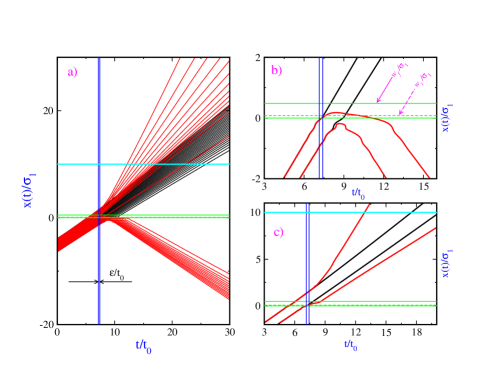
Figure 4: (Color online) a) A selection of Bohmian trajectories to have an overview of the problem, b) two typical reflected trajectories (in perturbed situation) and c) two typical transmitted paths. Black (red) trajectories are for the static (perturbed) situation. Vertical blue lines show the beginning and the end of perturbation, horizontal green lines show the borders of the barrier and the horizontal cyan line shows the detector place.

III Gaussian wavepacket and nonlinear increase in barrier height

It has been shown that during a finite time interval the time-varying probability of transmission exceeds that for free propagation in the scattering of a Gaussian wavepacket by a barrier with a height in linear increase MaMaHoPLA-2002 ; MaHo-Pranama-2002 . As the first generalization, we consider a situation where the height of the rectangular barrier changes nonlinearly in time from $0$ to $V_{0}$ as follows,

$$V(x,t) = V_{0}\hskip 2.84526pt\theta(x+\dfrac{w}{2})\hskip 2.84526pt\theta(\dfrac{w}{2}-x)$$

$$\times \begin{cases}0&\text{if}\hskip 2.84526ptt\leq t_{p}\\ a\left(\dfrac{t-t_{p}}{\varepsilon}\right)+b\left(\dfrac{t-t_{p}}{\varepsilon}\right)^{2}&\text{if}\hskip 2.84526ptt_{p}<t\leq t_{p}+\varepsilon\\ 1&\text{if}\hskip 2.84526ptt>t_{p}+\varepsilon\end{cases}$$

From Eq. (2) one obtains

$$T_{\text{f}} = \frac{1}{2}\left\{1+{\text{Erf}}{\left(\frac{p_{0}~{}t/m+x_{0}-x_{d}}{\sqrt{2}\sigma_{t}}\right)}\right\}~{},$$ (8)

for the time-varying transmission probability in free propagation, where $\sigma_{t}=\sqrt{1+(\hbar t/2m\sigma_{0}^{2})^{2}}$ is the rms width of the time-evolving wavepacket. In our calculations we have imposed constraints $a+b=1$, $0\leq a\leq 1$ and $0\leq b\leq 1$. In Fig. 5a) we have plotted time-evolving transmission probability for $a=0.1$ and $b=0.9$. Perturbation takes place during the time interval $[7.14t_{0},7.41t_{0}]$ where the height of barrier increases nonlinearly from $0$ to $2E_{0}$ and we have put $x_{d}=10\sigma_{1}$ and $w=0.32\sigma_{1}$.

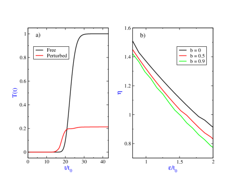
Figure 5: (Color online) Scattering of a Gaussian packet by a barrier with a height in nonlinear increase: a) Time evolution of transmission probability for the free (black curve) and perturbed case (red curve) with $a=0.1$ and $b=0.9$. b) Superarrivality versus duration of perturbation for three different values of non-linear coefficient.

In order to show dependence of superarrivals on the nonlinear coefficient $b$, we have plotted $\eta$ versus $\varepsilon$ in figure 5b) for three different values of $b$. As shown in this figure $\eta$ decreases with $\varepsilon$ ($b$) for a given value of $b$ ($\varepsilon$). When the height of the barrier increases in the nonlinear form (III), the rate of the change of barrier’s height is $V_{0}[\frac{a}{\varepsilon}+\frac{2(1-a)}{\varepsilon^{2}}(t-t_{p})]$ in contrast to the constant rate $\frac{V_{0}}{\varepsilon}$ in the case of linear increase. Thus for $t<t_{p}+\frac{\varepsilon}{2}$ ($t>t_{p}+\frac{\varepsilon}{2}$) the rate of increase is higher (lower) in the case of the non-linear perturbation than for the linear one. This means that in the first half of the perturbation when the incident packet has considerable interaction with the barrier, the potential changes slower compared to the linear increase and thus the kick the packet receives is weaker. As a result superarrivals are suppressed compared to the linear increase.

At the end we just briefly provide our numerical results in two more general cases: (i) in the scattering of a Gaussian wavepacket from two successive rectangular potential barriers which are perturbed by simultaneous increase in height, magnitude of superarrivals decreases with separation of barriers and duration of their perturbation, while increases with the final height of the barriers (ii) in the scattering of the non-Gaussian wavepacket ChHoMaMoMoSi-CQG-2012

$$\psi_{0}(x) = \frac{1+\alpha\sin\left(\frac{\pi(x-x_{0})}{4\sigma_{0}}\right)}{\sqrt{\sqrt{2\pi\sigma_{0}^{2}}\left[1+\alpha^{2}e^{-\pi^{2}/16}\sinh(\dfrac{\pi^{2}}{16})\right]}}$$ (9)

$$\times \exp\left[{-\dfrac{(x-x_{0})^{2}}{4\sigma_{0}^{2}}+i\dfrac{p_{0}}{\hbar}(x-x_{0})}\right]~{},$$

from a barrier with a height in linear increase, magnitude of superarrivals decreases with the duration of perturbation but does not have regular behavior with the non-Gaussian coefficient $\alpha$.

IV summary and discussion

In this paper we studied superarrivals in the scattering of a wavepacket from time-dependent rectangular potential barriers. We showed that superarrivals in transmission probability occurs in the scattering of a Gaussian wavepacket from a rectangular potential barrier with a width in linear increase during a finite time interval. Moreover, we depicted that the magnitude of superarrivals decreases with the duration of perturbation while grows when the final width of the perturbed barrier or detector distance from the barrier increases. By calculating the time evolution of Hamiltonian, momentum and position expectation values, we depicted that when the barrier’s width increases, the velocity of transmitted packet increases and yields superarrivals in transmission probability. We saw the effect of the perturbation is to reflect more trajectories and to push those that manage to pass the barrier by computing a selection of Bohmian trajectories.

We saw when the height of the barrier increases nonlinearly, the magnitude of superarrivals decreases with the nonlinear coefficient. From the above studies one sees that irrespective of the shape of the incident wavepacket (Gaussian/non-Gaussian) and the form of perturbation (linear/nonlinear), superarrivality decreases with the duration of the perturbation. The reason is as follows. Larger values of $\varepsilon$ correspond to slower changes in barrier. Thus, incident wavepacket will see a small change in the height/width of the barrier during its interaction with the barrier. As a result transmission probability will not be very different from that of the static barrier and thus superarrivality diminishes. This situation characterizes adiabatic limit in quantum mechanics.

References

- (1) M. Moshinsky, Phys. Rev. 88 (1952) 625.
- (2) S. Bandyopadhyay, A. S. Majumdar and D Home, Phys. Rev. A 65 (2002) 052718.
- (3) A. S. Majumdar and D. Home, Pramana-J. Phys. 59 (2002) 321.
- (4) Md. Manirul Ali, A. S. Majumdar and D. Home, Phys. Lett. A 304 (2002) 61.
- (5) D. Home, A. S. Majumdar and A. Matzkin, J. Phys. A:Math. Theor. 45 (2012) 295301.
- (6) P. R. Holland, (Cambridge University press, Cambridge, 1993).
- (7) C. R. Leavens C R, Phys. Lett. A 178 (1993) 27.
- (8) P. Chowdhury, D. Home, A.S. Majumdar, S.V. Mousavi, M.R. Mozaffari, S. Sinha, Class. Quantum. Grav. 29 (2012) 025010.