On the Frequency of Potential Venus Analogs from Kepler Data

Abstract

The field of exoplanetary science has seen a dramatic improvement in sensitivity to terrestrial planets over recent years. Such discoveries have been a key feature of results from the Kepler mission which utilizes the transit method to determine the size of the planet. These discoveries have resulted in a corresponding interest in the topic of the Habitable Zone (HZ) and the search for potential Earth analogs. Within the Solar System, there is a clear dichotomy between Venus and Earth in terms of atmospheric evolution, likely the result of the large difference ($\sim$ factor of two) in incident flux from the Sun. Since Venus is 95% of the Earth’s radius in size, it is impossible to distinguish between these two planets based only on size. In this paper we discuss planetary insolation in the context of atmospheric erosion and runaway greenhouse limits for planets similar to Venus. We define a “Venus Zone” (VZ) in which the planet is more likely to be a Venus analog rather than an Earth analog. We identify 43 potential Venus analogs with an occurrence rate ($\eta_{\venus}$) of $0.32^{+0.05}_{-0.07}$ and $0.45^{+0.06}_{-0.09}$ for M dwarfs and GK dwarfs respectively.

1. Introduction

The sensitivity of exoplanet detection instrumentation and techniques has dramatically improved over the past decade. This has enabled significant progress towards the detection of terrestrial-sized exoplanets using the radial velocity and transit methods. In particular, the Kepler mission has yielded a plethora of exoplanet candidates (Borucki et al., 2011a, b; Batalha et al., 2013; Burke et al., 2014), many of which have been confirmed by virtue of their multiplicity (Lissauer et al., 2014; Rowe et al., 2014). The primary purpose of the Kepler mission is to determine the frequency of Earth-sized planets in the Habitable Zone (HZ), which is the region around a star where water can exist in a liquid state on the surface of a planet with sufficient atmospheric pressure. Several Earth-sized planets have been located in this region as a result of these Kepler observations (Borucki et al., 2012; Quintana et al., 2014).

The inner and outer boundaries of the HZ for various main sequence stars have been estimated using one-dimensional climate models by Kasting et al. (1993). These boundary estimates have been revised in recent years by the same group, including the extension to later spectral types (Kopparapu et al., 2013) and the consideration of different planetary masses (Kopparapu et al., 2014). The HZ calculations are available through the Habitable Zone Gallery (Kane & Gelino, 2012a), which provides HZ calculations for all known exoplanetary systems. An important aspect of these HZ calculations is that they provide a means to estimate the fraction of stars with Earth-size planets in the HZ, or $\eta_{\oplus}$. Much of the recent calculations of $\eta_{\oplus}$ utilize Kepler results since these provide a large sample of terrestrial size objects from which to perform meaningful statistical analyses (Dressing & Charbonneau, 2013; Kopparapu, 2013; Petigura et al., 2013; Traub, 2012).

The transit method has a dramatic bias towards the detection of planets which are closer to the host star than farther away (Kane & von Braun, 2008). For example, the geometric transit probabilities of Mercury, Venus, and Earth for an external observer are 1.2%, 0.64%, and 0.46% respectively. Additionally, a shorter orbital period will result in an increased signal-to-noise (S/N) of the transit signature due to the increased number of transits observed within a given timeframe. The consequence of this is that Kepler has preferentially detected planets interior to the HZ which are therefore more likely to be potential Venus analogs than Earth analogs. An example of this is Kepler-69c which was initially thought to be a strong HZ candidate (Barclay et al., 2013) but subsequent analysis showed that it’s more likely to be a super-Venus (Kane et al., 2013). Since the divergence of the Earth/Venusian atmospheric evolutions is a critical component for understanding Earth’s habitability, the frequency of Venus analogs ($\eta_{\venus}$) is also important to quantify.

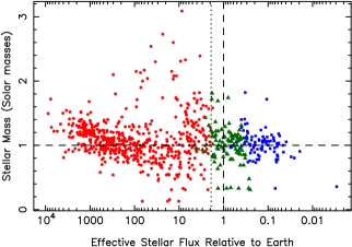
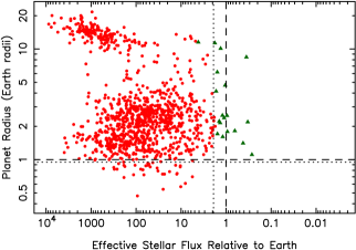
Figure 1.— The dependence of effective stellar flux received by the planet on stellar mass (left) and planet radius (right). The green triangles are those planets which spend more than 50% of their orbital phase within the optimistic Habitable Zone. The red circles and blue squares are planets interior and exterior to the Habitable Zone respectively. The dashed crosshairs show the location of Earth, and the dotted crosshairs show the location of Venus. The right-hand plot includes only those planets for which a radius determination is available.

Here we provide a definition for the Venus Zone (VZ) and an estimate for $\eta_{\venus}$ by examining the frequency of Venus analogs from Kepler data. In Section 2 we discuss the current insolation distribution of exoplanets based upon confirmed exoplanet discoveries. In Section 3 we describe the outer boundary of the VZ in terms of the runaway greenhouse limit (Section 3.1) and the inner VZ boundary using an estimate of the atmospheric erosion limit (Section 3.2). In Section 4 we present calculations of $\eta_{\venus}$ using exoplanet candidates from the Kepler mission. Finally, we provide concluding remarks in Section 5.

2. The Planetary Insolation Distribution

Exoplanets have been discovered at a variety of distances around different kinds of stars. However, even without direct knowledge of planetary surface conditions, one can still calculate the HZ of a star based on Earth models. For example, the models of Kasting et al. (1993) and Kopparapu et al. (2013, 2014) quantify incident fluxes that would cause planetary temperature conditions to sway to either a runaway greenhouse effect or to a runaway snowball effect. For a given planet, these calculations are based upon the stellar effective temperature, stellar flux, and water absorption by the atmosphere. The flux thresholds at which these transitions from one planetary state to another occur allow for both conservative and optimistic scenarios depending on how long it is presumed that Venus and Mars were able to retain liquid water on their surfaces. Here we adopt the “conservative” and “optimistic” models of Kane et al. (2013). The conservative model uses the “Runaway Greenhouse” and “Maximum Greenhouse” criteria for the inner and outer HZ boundaries respectively. The optimistic model uses the “Recent Venus” and “Early Mars” criteria for the inner/outer HZ boundaries. These criteria are described in detail by Kopparapu et al. (2013, 2014).

The insolation (stellar flux received relative to Earth) distribution for exoplanets are summarized in Figure 1. The required stellar and planetary data for confirmed exoplanets were extracted from the Exoplanet Data Explorer (Wright et al., 2011). The data are current as of 21st June 2014. In each plot, the red circles represent those planets interior to the optimistic HZ and the blue squares those planets exterior to the HZ. The green triangles represent those planets which spend more the 50% of their orbital phase within the optimistic HZ, keeping in mind that some of these planets lie in eccentric orbits. The dashed crosshairs indicate Earth’s position in the plots for comparison.

The stellar mass vs insolation plot (Figure 1, left) appears to contain a trend from high flux at high stellar mass to low flux at low stellar mass. This is due to observational bias since low-mass planets at longer orbital periods fall under current detection thresholds. Figure 1 (right) includes only those planets for which a radius determination is available. The distinct giant and terrestrial planet populations at high incident fluxes is made clear in this figure, which is likely a result of planet formation/migration mechanisms. More importantly, this figure is the key for determining $\eta_{\oplus}$ which can be thought of as the relative number of points near the cross-hairs (Earth). As this figure continues to fill out, it will be the clearest indicator of the prevalence of Earth-analogs.

Another compelling question that arises from the plots in Figure 1 is: how many of the points represent potential Venus analogs as that is clearly where detection is currently more efficient? In other words, missions such as Kepler are more capable of determining $\eta_{\venus}$ than $\eta_{\oplus}$. Since Venus and Earth are approximately the same size, the Venus analogs will emerge earlier than the Earth analogs due to the increased geometric transit probability (Kane & von Braun, 2008). The location of Venus on the plots is indicated by dotted crosshairs. The solar flux received by the Earth is approximately 1365 W/m² and the flux received by Venus is 2611 W/m², thus Venus receives 1.91 times more flux than the Earth. In order to determine $\eta_{\venus}$, we must first define boundaries for the Venus Zone.

3. Defining the Venus Zone Boundaries

Here we describe approximate boundaries for the Venus Zone (VZ) which will be subsequently be used to estimate $\eta_{\venus}$.

3.1. Outer Venus Boundary: Runaway Greenhouse

The outer boundary of the VZ is defined by the limit where oceans will completely evaporate, leading to (for example) the apparent Venus/Earth dichotomy that we see within our Solar System. The precise mechanisms through which this takes place are complicated, but essentially the loss of liquid water results in the inability to execute a carbon cycle and thus efficiently moderate the levels of atmospheric carbon (CO₂). There are various ways in which surface temperature conditions might rise to such levels that would result in a runaway greenhouse. Barnes et al. (2013) suggested that tidal effects may result in Venus analogs through tidal heating, particularly for planets in eccentric orbits (Kane & Gelino, 2012b; Williams & Pollard, 2002). Here we consider only the effects of stellar flux on the potential for runaway greenhouse, as described by Kasting et al. (1993) and Kopparapu et al. (2013, 2014).

There are also a variety of ways in which the intrinsic properties of the planet will influence this boundary. The calculations of Kopparapu et al. (2013) do not include H₂O and CO₂ clouds, each of which have separate effects. H₂O clouds generally move the inner HZ boundary closer to the star (Leconte et al., 2013a; Wolf & Toon, 2014; Yang et al., 2013) but CO₂ clouds result in IR back-scattering thus increasing the surface temperature and moving the HZ outward through greenhouse warming. Models by Forget & Pierrehumbert (1997) and Selsis et al. (2007) show that the overall effect of neglecting clouds may result in an underestimate of the greenhouse effect. Abe et al. (2011) and Leconte et al. (2013b) describe how a planet may lose surface water and remain habitable as a “land planet”. Armstrong et al. (2014) further showed that certain ranges of obliquity will expand the HZ through seasonal variations, whilst Yang et al. (2014) demonstrated the dependence of the HZ inner edge on planetary rotation. However, the boundary at which water evaporation and runaway greenhouse will take hold is well approximated by the 1 M_⊕ Runaway Greenhouse of Kopparapu et al. (2014). We thus adopt this as the outer boundary of the VZ.

3.2. Inner Venus Boundary: Atmospheric Erosion

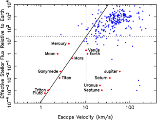
Figure 2.— Stellar flux (relative to Earth) received by various objects as a function of their escape velocities. Selected objects from the Solar System are shown as labeled red circles. The small blue squares represent exoplanets with sufficient planetary and stellar information. The dotted corsshairs show the incident flux needed for Venus to be at the “cosmic shoreline”.

Runaway greenhouse may be prevented if significant atmospheric mass loss occurs as a result of proximity to the host star. The role of extreme ultraviolet (XUV) radiation in atmospheric mass loss has been the subject of several studies (Lammer et al., 2009; Lopez et al., 2012; Lopez & Fortney, 2013). The XUV effect is applicable to terrestrial planets in high incident flux regimes (less than 10 day orbital periods). Here we adopt a simple approximation for the loss of an atmosphere based upon the work of Catling & Zahnle (2009, 2013) and referred to as the “cosmic shoreline” by Zahnle & Catling (2013). This is an empirical relationship between incident flux and surface gravity derived from observations of objects within the Solar System and then extrapolated to exoplanets. Figure 2 shows a new version of this relationship where selected Solar System objects are shown as red circles. Confirmed exoplanets for which sufficient data were available (see Section 2) are shown as blue squares. The solid line is a power-law approximation which separates those bodies with (right of the line) and without (left of the line) atmospheres. Many of the exoplanets that lie to the left of the line (blue squares) have high densities ($>5.5$ g/cm³), which if correct, would be consistent with iron-silicate composition. We find that the best approximation for the power-law is $I\propto v_{e}^{5.2}$ where $I$ is the incident flux and $v_{e}$ is the escape velocity. There are several caveats to note about this relationship between incident flux and atmospheric mass loss. There is an implicit assumption regarding the mean molecular weight of the atmospheric material which is being averaged to account for all atmospheric compositions. Furthermore, the timescale for atmospheric loss will vary depending on stellar mass and luminosity for a given planet. With these caveats in mind, we adopt the incident flux needed for Venus to be at the “cosmic shoreline” as an approximation for the inner boundary of the VZ; $\sim$ 25 times the Earth incident flux (see Figure 2).

4. The Frequency of Venus Analogs

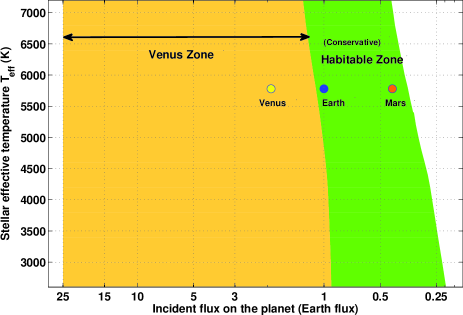
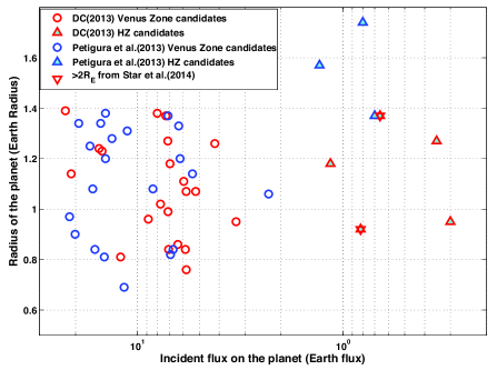
Figure 3.— Left: Incident stellar flux on a planet versus stellar effective temperature, showing the extent of the Venus Zone and (conservative) Habitable Zone. Right: Incident stellar flux on a planet versus planet radius. The data are from Dressing & Charbonneau (2013) (red circles and triangles) and Petigura et al. (2013) (blue circles and triangles). Planets in the HZ from both the data sets are in filled colors. There are a total of $43$ planets in the VZ. List of these candidates are provided in Tables 1 & 2. Two of the planets from Dressing & Charbonneau (2013) (red down triangles), KOI 1422.02 and KOI 2626.01, may be larger than $2$R_⊕, according to Star et al. (2014).

In this section, we will calculate the occurrence rate of terrestrial size planets that receive a flux which puts them between the runaway greenhouse limit and atmospheric erosion caused by incident stellar flux. We call this region the “Venus Zone” (VZ) to identify those exoplanets that are either in the runaway greenhouse state or in the process of losing their atmosphere due to the close proximity to their host star (see Section 3). The extent of the VZ and HZ boundaries are shown in the left panel of Figure 3 as a function of stellar effective temperature. We calculate the occurence rate of VZ planets for GKM stellar spectral types, using the data from Dressing & Charbonneau (2013) (for M-dwarfs) and Petigura et al. (2013) (for K & G-dwarfs). Both these studies calculate the planet occurrence rate based on the following equation:

$$f(R_{p},P) = \sum_{i=1}^{N_{p}(R_{p},P)}\frac{a_{i}}{R_{\star,i}N_{\star,i}}$$ (1)

where $a_{i}$ is the semi-major axis of planet $i$, $R_{\star,i}$ is the host star’s radius of planet $i$, $N_{\star,i}$ is the number of stars around which planet $i$ could have been detected and $N_{p}(R_{p},P)$ is the number of planets with the radius $R_{p}$ and period $P$. The ratio $a_{i}/R_{\star,i}$ is the inverse of the probability of transit orientation, which is considered to take non-transiting geometries into the estimation of occurrence rate. Petigura et al. (2013) use $N_{\star,i}=C\times n_{\star}$, where $C$ is the completeness correction factor for each $(P,R_{p})$ bin, and $n_{\star}=42,557$ stars in their survey of brightest (Kepler magnitude 10–15) GK spectral types.

To calculate the occurrence rate for M-dwarfs, we use the $N_{\star,i}$ values provided within the period-radii cells of Figure 15 of Dressing & Charbonneau (2013), which give the number of stars around which a planet from the center of the grid cell would have been detected with a signal-to-noise ratio above $7.1\sigma$. This should still give us nearly the same occurrence rate, or an underestimate of the actual value. This is because, as pointed by Kopparapu (2013), the $N_{\star,i}$ values calculated by Dressing & Charbonneau (2013) and used in their estimate of $\eta_{\oplus}$ are generally lower in value than the center of the grid cells values we use from Figure 15. If this is the general trend, i.e., if we are overestimating $N_{\star,i}$ systematically, then our calculated occurrence rates for M-dwarfs can be considered as a lower bound to the actual value.

In the case of occurrence rates for K & G-dwarfs, completeness correction factors from Petigura et al. (2013) are available (see Figure  S11, supplementary information). As mentioned above, they also provide $n_{\star}=42,557$ stars. Therefore, all the required values are available to calculate the occurrence rate using Equation 1.

We identify those planets that are in the appropriate period-radius bin from each data set. We consider planets with $0.5-1.4$R_⊕ as terrestrial size, and count all the planets in the VZ. Restricting the outer edge of VZ to the runaway greenhouse flux limit from Kopparapu et al. (2014) for different stars, and the inner edge to the empirical relation between stellar flux and planetary gravity for Venus from Figure 2 ($25$ times incident flux on Earth), there are 22 planets in the M-star sample of Dressing & Charbonneau (2013). With these conditions, using Equation 1, the occurrence rate of terrestrial size planets that are potentially Venus analogs around M-dwarfs is $0.32^{+0.05}_{-0.07}$. Similarly, there are $21$ planets in the K $\&$ G-star sample of Petigura et al. (2013) within the VZ. The corresponding occurrence rate around K $\&$ G-stars is $0.45^{+0.06}_{-0.09}$. The uncertainties are estimated by (1) calculating the effective number of stars searched (detected planets in the sample divided by the occurrence rate) (2) constructing a binomial cumulative distribution function (CDF) representing the likelihood of finding specified number of planets given the effective number of stars searched and the probability of finding a planet (i.e, occurrence rate), (3) finding the number of planets corresponding to the $15.9$ and $84.1$ percentiles in the CDF, (4) calculating the new occurrence rates by dividing the number of planets from percentile ranges with the effective number of stars searched and (5) finally subtracting these new rate bounds from the original rates. A list of all the planet candidates are provided in Tables 1 $\&$ 2. A comparison of the various classifications of the candidates as described here is shown in the right panel of Figure 3.

Several caveats are to be noted: (1) None of these are confirmed planets, and are only candidates. In fact, a recent study by Star et al. (2014) showed that two of the planet candidates (KOI 1422.02 and KOI 2626.01) in the HZ are larger than previous estimates. This may remove some planets out of contention and thus reduce the occurrence rate. The uncertainties in the stellar parameters and thus planetary radii are not well constrained, so this may also add to the uncertainty in our occurrence estimate (Kane, 2014). On the other hand, Dressing & Charbonneau (2013) used the Q1–Q6 sample. It is likely that an expanded dataset may increase the occurrence rate around M-dwarf stars. So the net effect may not change the rate estimate significantly. (2) We use an upper flux limit of $25$ times Earth flux. This number arises from Figure 2, by finding the intersection point for Venus on the “cosmic shoreline” (the solid line). Our terrestrial size planet has a radius range of $0.5-1.4$ R_⊕. Correspondingly, the flux limit can vary depending on the size (or gravity) of the planet. This in turn changes the occurrence rate (i.e, a planet with lower gravity has a lower flux limit, and hence a lower estimate of the occurrence rate). Our estimates above are in this sense an average value that encompasses the terrestrial size planets. (3) Although we define an outer boundary of the VZ, there are planetary properties that could push this out even further, such as sufficiently increased CO₂ levels that could push an atmosphere into runaway greenhouse even at larger distances. However, the probability of runaway greenhouse will start to drop dramatically with increasing distance beyond the VZ. Thus, our calculation of $\eta_{\venus}$ using the defined VZ likely encompasses most Venus analogs. (4) Just as planets in the HZ should be considered “Earth-like candidates” until their properties can be confirmed via spectroscopy, planets inside the VZ should be considered “Venus-like candidates” until spectral measurements and characterization efforts are undertaken.

Table 1 List of M-dwarf KOIs that are terrestrial in size ($0.5-1.4$ R_⊕) and which receive a stellar flux between runaway greenhouse limit and atmospheric erosion. Data from Dressing & Charbonneau (2013).

KOI	Radius ($R_{\oplus}$)	Period (days)	$T_{\mathrm{eff}}$ (K)	Flux ($F_{\oplus}$)
$251.02$	$0.76^{+0.08}_{-0.10}$	$5.78$	$3743.0$	$16.81$
$571.01$	$1.37^{+0.14}_{-0.21}$	$7.27$	$3820.0$	$13.98$
$571.04$	$1.39^{+0.14}_{-0.21}$	$22.41$	$3820.0$	$3.12$
$886.01$	$1.38^{+0.30}_{-0.27}$	$8.01$	$3579.0$	$5.30$
$886.02$	$0.81^{+0.18}_{-0.16}$	$12.07$	$3579.0$	$3.07$
$886.03$	$1.14^{+0.25}_{-0.22}$	$21.00$	$3579.0$	$1.47$
$899.01$	$1.27^{+0.15}_{-0.25}$	$7.11$	$3587.0$	$8.74$
$899.02$	$0.95^{+0.12}_{-0.19}$	$3.31$	$3587.0$	$24.26$
$899.03$	$1.24^{+0.15}_{-0.24}$	$15.37$	$3587.0$	$3.13$
$1085.01$	$1.02^{+0.11}_{-0.10}$	$7.72$	$3878.0$	$14.89$
$1146.01$	$0.99^{+0.13}_{-0.10}$	$7.10$	$3778.0$	$12.32$
$1422.01$	$0.84^{+0.19}_{-0.19}$	$5.84$	$3424.0$	$4.20$
$1681.01$	$1.18^{+0.18}_{-0.15}$	$6.94$	$3608.0$	$8.63$
$1843.01$	$1.26^{+0.14}_{-0.22}$	$4.20$	$3584.0$	$19.30$
$1843.02$	$0.86^{+0.10}_{-0.15}$	$6.36$	$3584.0$	$11.09$
$1867.03$	$1.07^{+0.11}_{-0.12}$	$5.21$	$3799.0$	$20.76$
$2036.02$	$1.07^{+0.10}_{-0.20}$	$5.79$	$3903.0$	$21.85$
$2057.01$	$1.11^{+0.10}_{-0.14}$	$5.95$	$3900.0$	$21.67$
$2179.01$	$1.23^{+0.15}_{-0.18}$	$14.87$	$3591.0$	$3.20$
$2191.01$	$0.96^{+0.11}_{-0.13}$	$8.85$	$3724.0$	$8.61$
$2650.01$	$1.18^{+0.40}_{-0.15}$	$34.99$	$3735.0$	$1.15$
$2650.02$	$0.84^{+0.29}_{-0.11}$	$7.05$	$3735.0$	$9.73$

Table 2 List of K $\&$ G-dwarf KOIs that are terrestrial in size ($0.5-1.4$ R_⊕) and which receive a stellar flux between runaway greenhouse limit and atmospheric erosion. Data from Petigura et al. (2013).

KIC ID	KOI	Radius ($R_{\oplus}$)	Period (days)	$T_{\mathrm{eff}}$ (K)	Flux ($F_{\oplus}$)
$1849702$	$2538.01$	$1.37$	$39.83$	$5023.0$	$7.1$
$3223433$	$4548.01$	$1.20$	$61.08$	$5518.0$	$6.2$
$4276716$	$1619.01$	$0.81$	$20.66$	$4882.0$	$14.5$
$5374403$	$2556.01$	$1.38$	$40.84$	$5523.0$	$14.3$
$5706966$	$1908.01$	$1.28$	$12.55$	$4350.0$	$13.3$
$5780930$	$3412.01$	$1.20$	$16.75$	$4683.0$	$14.3$
$7742408$	$0.00$	$0.84$	$33.50$	$4802.0$	$6.7$
$8349399$	$4763.01$	$1.25$	$56.45$	$5980.0$	$17.0$
$8481129$	$2402.01$	$1.08$	$16.30$	$4763.0$	$16.5$
$8560940$	$3450.01$	$0.97$	$31.97$	$5852.0$	$21.4$
$8625732$	$4701.01$	$0.84$	$31.97$	$5597.0$	$16.1$
$9116075$	$0.00$	$0.82$	$24.50$	$4570.0$	$6.9$
$9150827$	$1408.01$	$1.08$	$14.53$	$4252.0$	$8.4$
$9334893$	$2298.01$	$0.90$	$16.67$	$4922.0$	$20.1$
$9412760$	$1977.01$	$1.34$	$9.39$	$4346.0$	$19.3$
$9718066$	$2287.01$	$0.69$	$16.09$	$4470.0$	$11.6$
$9993683$	$0.00$	$1.34$	$29.94$	$5241.0$	$15.1$
$10453588$	$2484.01$	$1.31$	$68.89$	$5739.0$	$11.2$
$11462341$	$2124.01$	$1.06$	$42.34$	$4252.0$	$2.3$
$11774991$	$2173.01$	$1.14$	$37.81$	$4705.0$	$5.4$
$12735830$	$3311.01$	$1.33$	$31.83$	$4712.0$	$6.3$

5. Conclusions

A critical question that exoplanet searches are attempting to answer is: how common are the various elements that we find within our own Solar System? This includes the determination of Jupiter analogs since the giant planet has undoubtedly played a significant role in the formation and evolution of our Solar System. When considering the terrestrial planets, the attention often turns to atmospheric composition and prospects of habitability. In this context, the size degeneracy of Earth with its sister planet Venus cannot be ignored and the incident flux must be carefully considered. Here we have provided a definition for a region where terrestrial planets are potentially Venus analogs using data from Solar System bodies. This results in the first estimate of $\eta_{\venus}$; the frequency of Venus/Earth-size planets within the VZ. The occurrence rates are similar to those of $\eta_{\oplus}$ though with significantly smaller uncertainties since Kepler is more biased towards planets in the VZ compared with the HZ. Future missions capable of identifying key atmospheric abundances for terrestrial planets will face the challenge of distinguishing between possible Venus and Earth-like surface conditions. Discerning the actual occurrence of Venus analogs will help us to decode why the atmosphere of Venus so radically diverged from its sister planet, Earth.

References

- Abe et al. (2011) Abe, Y., Abe-Ouchi, A., Sleep, N.H., Zahnle, K.J. 2011, AsBio, 11, 443
- Armstrong et al. (2014) Armstrong, J.C., Barnes, R., Domagal-Goldman, S., Breiner, J., Quinn, T.R., Meadows, V.S. 2014, AsBio, 14, 277
- Barclay et al. (2013) Barclay, T., et al. 2013, ApJ, 768, 101
- Barnes et al. (2013) Barnes, R., Mullins, K., Goldblatt, C., Meadows, V.S., Kasting, J.F., Heller, R. 2013, AsBio, 13, 225
- Batalha et al. (2013) Batalha, N.M., et al., 2013, ApJS, 204, 24
- Borucki et al. (2011a) Borucki, W.J., et al., 2011a, ApJ, 728, 117
- Borucki et al. (2011b) Borucki, W.J., et al., 2011b, ApJ, 736, 19
- Borucki et al. (2012) Borucki, W.J., et al., 2012, ApJ, 745, 120
- Burke et al. (2014) Burke, C.J., et al. 2014, ApJS, 210, 19
- Catling & Zahnle (2009) Catling, D.C., Zahnle, K.J. 2009, SciAm, 300, 36
- Catling & Zahnle (2013) Catling, D.C., Zahnle, K.J. 2013, LPSC, 44, 2665
- Dressing & Charbonneau (2013) Dressing, C.D., Charbonneau, D. 2013, ApJ, 767, 95
- Forget & Pierrehumbert (1997) Forget, F., Pierrehumbert, R.T. 1997, Science, 278, 1273
- Kane & von Braun (2008) Kane, S.R., von Braun, K. 2008, ApJ, 689, 492
- Kane & Gelino (2012a) Kane, S.R., Gelino, D.M. 2012a, PASP, 124, 323
- Kane & Gelino (2012b) Kane, S.R., Gelino, D.M. 2012b, AsBio, 12, 940
- Kane et al. (2013) Kane, S.R., Barclay, T., Gelino, D. 2013, ApJ, 770, L20
- Kane (2014) Kane, S.R. 2014, ApJ, 782, 111
- Kasting et al. (1993) Kasting, J.F., Whitmire, D.P., Reynolds, R.T. 1993, Icarus, 101, 108
- Kopparapu et al. (2013) Kopparapu, R.K., et al. 2013, ApJ, 765, 131
- Kopparapu (2013) Kopparapu, R.K., 2013, ApJ, 767, L8
- Kopparapu et al. (2014) Kopparapu, R.K., et al. 2014, ApJ, 787, L29
- Lammer et al. (2009) Lammer, H., et al. 2009, A&A, 506, 399
- Leconte et al. (2013a) Leconte, J., Forget, F., Charnay, B., Wordsworth, R., Pottier, A. 2013a, Nature, 504, 268
- Leconte et al. (2013b) Leconte, J., Forget, F., Charnay, B., Wordsworth, R., Selsis, F., Millour, E., Spiga, A. 2013b, A&A, 554, 69
- Lissauer et al. (2014) Lissauer, J.J., et al. 2014, ApJ, 784, 44
- Lopez et al. (2012) Lopez, E.D., Fortney, J.J., Miller, N. 2012, ApJ, 761, 59
- Lopez & Fortney (2013) Lopez, E.D., Fortney, J.J. 2013, ApJ, 776, 2
- Petigura et al. (2013) Petigura, E.A., Howard, A.W., Marcy, G.W. 2013, PNAS, 110, 19273
- Quintana et al. (2014) Quintana, E.V., et al. 2014, Science, 344, 277
- Rowe et al. (2014) Rowe, J.F., et al. 2014, ApJ, 784, 45
- Selsis et al. (2007) Selsis, F., Kasting, J.F., Levrard, B., Paillet, J., Ribas, I., Delfosse, X., 2007, A&A, 476, 1373
- Star et al. (2014) Star, K.M., Gilliland, R.L., Wright, J.T., Ciardi, D.R. 2014, ApJ, submitted (arXiv:1407.1057)
- Traub (2012) Traub, W. 2012, ApJ, 745, 20
- Williams & Pollard (2002) Williams, D.M., Pollard, D. 2002, IJAsB, 1, 61
- Wolf & Toon (2014) Wolf, E., Toon, O.B. 2014, Geophysical Research Letters, 41, 167
- Wright et al. (2011) Wright, J.T., et al. 2011, PASP, 123, 412
- Yang et al. (2013) Yang, J., Cowan, N.B., Abbot, D.S. 2013, ApJ, 771, L45
- Yang et al. (2014) Yang, J., Boué, G., Fabrycky, D.C., Abbot, D.S. 2014, ApJ, 787, L2
- Zahnle & Catling (2013) Zahnle, K.J., Catling, D.C. 2013, LPSC, 44, 2787