A Low Mach Number Model for Moist Atmospheric Flows

Abstract

We introduce a low Mach number model for moist atmospheric flows that accurately incorporates reversible moist processes in flows whose features of interest occur on advective rather than acoustic time scales. Total water is used as a prognostic variable, so that water vapor and liquid water are diagnostically recovered as needed from an exact Clausius–Clapeyron formula for moist thermodynamics. Low Mach number models can be computationally more efficient than a fully compressible model, but the low Mach number formulation introduces additional mathematical and computational complexity because of the divergence constraint imposed on the velocity field. Here, latent heat release is accounted for in the source term of the constraint by estimating the rate of phase change based on the time variation of saturated water vapor subject to the thermodynamic equilibrium constraint. We numerically assess the validity of the low Mach number approximation for moist atmospheric flows by contrasting the low Mach number solution to reference solutions computed with a fully compressible formulation for a variety of test problems.

1 Introduction

Small–scale atmospheric phenomena are typically characterized by relatively slow dynamics, that is, low Mach number flows for which the fast acoustic modes are physically irrelevant. Thus, numerical modeling of these flows does not typically require explicitly resolving fast–propagating sound waves. Two different approaches have been widely used to remove the time step constraint that would result from resolving fast acoustic modes. The first and more common approach solves the fully compressible equations of motion but limits the impact of acoustic modes, for instance, by advancing the acoustic signal in time with an implicit time discretization or with multiple smaller time steps, as originally considered for cloud models in [TW76] and [KW78]. A second alternative consists of analytically filtering acoustic modes from the original compressible equations, thus deriving a new set of equations, often called sound–proof equations. Within this category are anelastic [Bat53, OP62, DF69, Gou69] and pseudo–incompressible [Dur89] models.

Several anelastic formulations (see, e.g., [Cla79, LH82, GS02]), and recently a pseudo–incompressible formalism [OK14], have been developed for moist flows. In this paper we derive a low Mach number model for moist atmospheric flows with a general equation of state using the low Mach number formalism in [ABNZ08] as a starting point. Here we use the term “low Mach number model” to refer to a model in which the equations are valid approximations to the fully compressible equations when the Mach number is small. In atmospheric modeling, the equations which follow from assuming the Mach number is small, thus the variation of the pressure from the background pressure is small, are also referred to as pseudo–incompressible equations following [Dur89]. The anelastic equations require additional assumptions on the smallness of density and temperature variations to be valid. (For a complete discussion on sound-proof equations for atmospheric flows, and their differences, see, for instance, [Kle09] and references therein.) We note that the low Mach number equations presented here do not guarantee that a flow that initially satisfies the low Mach number assumption will continue to satisfy it for all time. The buoyancy forcing from a large density perturbation in a domain with large vertical extent could accelerate the flow into a regime where the Mach number is no longer small. Once the flow reached this regime, the low Mach number equations would no longer be valid approximations to the fully compressible equations. However, until that point, the equations are valid.

Analogous to the moist pseudo–incompressible model of [OK14] we consider only reversible processes given by water phase changes, using here an exact Clausius–Clapeyron formula for moist thermodynamics. In contrast to [OK14], however, we derive the equations of motion in terms of conserved variables (like [Ooy90] in a compressible framework), that is, using appropriate invariant variables such that terms resulting from phase change are eliminated from the time evolution equations [Bet73, TC81, HH89]. We also include the effects of the specific heats of both water vapor and liquid water, and consider an isentropic expansion factor ($\gamma$) that accounts for variations in the water composition of moist air. Although the low Mach number formulation holds for any moist equation of state, for the purposes of numerical comparison with compressible solutions we consider the special case where both dry air and water vapor are assumed to be ideal gases.

While the larger time step allowed by the low Mach number formulation can lead to greater computational efficiency than a purely compressible formulation, it may also introduce larger errors in the dynamics of moist flows as investigated in [DAB⁺14]. In addition to the latent heat release accompanying phase changes, thermodynamic properties such as the specific heat of moist air, as well as thermodynamic variables such as temperature, depend on the composition of the moist air, thus change over the time step. This motivates our use of invariant variables as prognostic variables, namely total water content and a specific enthalpy of moist air that accounts for both sensible and latent heats. In models where source terms related to phase transition appear explicitly in the evolution equations, they are typically first neglected or lagged in time and then corrected or estimated during a given time step; the use of invariant variables removes the need of accounting for such terms. Nevertheless, the diabatic contribution of the latent heat release must appear in the source term for the low Mach divergence constraint on the velocity field. In practice the latter involves computing the rate of evaporation (or condensation). Since no analytical expression exists for this rate, one of the most common ways to estimate it deduces it from the change in water vapor content necessary to ensure that there is no supersaturated water vapor at the end of the time step (cf. [SO73]). This variation is measured with respect to an initial estimate of water vapor that does not necessarily respect the saturation requirements either because it was initially advected without accounting for phase changes (see, e.g., [KW78, GS90, BF02, Sat03, OK14]) or because it considers a lagged evaporation rate from the previous time step (see, e.g., [GS02]). In our model, because water vapor is not used as a prognostic variable, we cannot compute this variation of water vapor. Instead we adopt a different approach, similar to [LH82], that estimates the evaporation rate based on the fact that whenever a parcel is saturated, a Clausius–Clapeyron formula relates the local values of water content to the thermodynamics within the parcel. The conservation equation for saturated water vapor then becomes a time–varying constraint that guarantees thermodynamic equilibrium from which the evaporation rate can be estimated. The latter is thus computed as required during a time step using the current values of water content and thermodynamic variables, diagnostically recovered from the invariant prognostic variables.

This paper is organized as follows. We introduce the new low Mach number model for moist atmospheric flows in Section 2, and describe the moist thermodynamics in Section 3. In Section 4 we discuss the numerical implementation. Finally, in Section 5, we present several numerical comparisons and discuss our findings.

2 Low Mach number formulation

We begin by writing the fully compressible equations of motion expressing conservation of mass, momentum, and enthalpy in a constant gravitational field in which we neglect Coriolis forces and viscous terms:

$$\frac{\partial\rho}{\partial t}+\boldsymbol{\nabla}\boldsymbol{\cdot}\left(\rho\boldsymbol{U}\right) = 0,$$ (1)

$$\frac{\partial\left(\rho\boldsymbol{U}\right)}{\partial t}+\boldsymbol{\nabla}\boldsymbol{\cdot}\left(\rho\boldsymbol{U}\boldsymbol{U}\right)+\boldsymbol{\nabla}p = -\rho g\boldsymbol{\hat{e}}_{z},$$ (2)

$$\frac{\partial(\rho\widehat{h})}{\partial t}+\boldsymbol{\nabla}\boldsymbol{\cdot}(\rho\widehat{h}\boldsymbol{U})-\frac{Dp}{Dt} = \rho\mathcal{H},$$ (3)

where the material derivative is defined as $D/Dt=\partial/\partial t+\boldsymbol{U}\boldsymbol{\cdot}\boldsymbol{\nabla}$. Here $\rho$ is the total density, $\boldsymbol{U}$ is the velocity, and $\widehat{h}$ is the specific enthalpy of moist air. The pressure, $p$, is defined by an equation of state (EOS). The term $\mathcal{H}$ represents a source of heat (per unit mass and time) to the system, such as thermal conduction or radiation. We include gravitational acceleration given by $\boldsymbol{g}=-g\boldsymbol{\hat{e}}_{z}$, where $\boldsymbol{\hat{e}}_{z}$ is the unit vector in the vertical direction.

We formulate the moist atmospheric processes as in [Rom08], with the additional simplification that at any grid point all phases have the same velocity and temperature. We treat moist air as an ideal mixture of dry air, water vapor, and liquid water, with the water phases in thermodynamic equilibrium, so that only reversible processes are taken into account; ice–phase microphysics, precipitation fallout, and subgrid–scale turbulence are ignored. Denoting by $q_{a}$, $q_{v}$, and $q_{l}$ the mass fraction of dry air, water vapor, and liquid water, respectively, we note that $q_{a}+q_{v}+q_{l}=1$ and write

$$\frac{\partial\left(\rho q_{a}\right)}{\partial t}+\boldsymbol{\nabla}\boldsymbol{\cdot}\left(\rho q_{a}\boldsymbol{U}\right) = 0,$$ (4)

$$\frac{\partial\left(\rho q_{v}\right)}{\partial t}+\boldsymbol{\nabla}\boldsymbol{\cdot}\left(\rho q_{v}\boldsymbol{U}\right) = e_{v},$$ (5)

$$\frac{\partial\left(\rho q_{l}\right)}{\partial t}+\boldsymbol{\nabla}\boldsymbol{\cdot}\left(\rho q_{l}\boldsymbol{U}\right) = -e_{v},$$ (6)

where $\rho$ is the total density. Positive values of $e_{v}$ correspond to evaporation; negative values correspond to condensation. If we define the mass fraction of total water, $q_{w}=q_{v}+q_{l}$, then we can replace (5)–(6) by

$$\frac{\partial\left(\rho q_{w}\right)}{\partial t}+\boldsymbol{\nabla}\boldsymbol{\cdot}\left(\rho q_{w}\boldsymbol{U}\right)=0.$$ (7)

(We note that the system including both (1) and (4)–(6) or (1), (4), and (7) is over–specified; in practice (1) need not be solved separately.)

We define the internal energy of moist air, $\widehat{e},$ as in [Rom08],

$$\widehat{e}=c_{vm}\left(T-T_{\mathrm{trip}}\right)+q_{v}E_{0v},$$ (8)

where the constant–volume specific heat of moist air is given by $c_{vm}=q_{a}c_{va}+q_{v}c_{vv}+q_{l}c_{vl},$ with the specific heats at constant volume: $c_{va}$, $c_{vv}$, and $c_{vl}$, for dry air, water vapor, and liquid water, respectively. Here $T_{\mathrm{trip}}$ is the triple–point temperature and $E_{0v}$ is the specific internal energy of water vapor at the triple point, while the enthalpy of moist air is given by

$$\widehat{h}=\widehat{e}+\frac{p}{\rho}.$$ (9)

Note that an evolution equation for the internal energy

$$\frac{\partial\left(\rho\widehat{e}\right)}{\partial t}+\boldsymbol{\nabla}\boldsymbol{\cdot}\left(\rho\widehat{e}\boldsymbol{U}\right)+p\left(\boldsymbol{\nabla}\boldsymbol{\cdot}\boldsymbol{U}\right)=\rho\mathcal{H},$$ (10)

can be used instead of (3). In either case, there are no source terms related to phase change in (3) or (10), as observed in [Ooy90] and [DAB⁺14]. Finally, to close the system (1)–(4) with (7), we consider a general equation of state for moist air written as $p=p(\rho,T,q_{a},q_{v},q_{l})$. (Because $q_{a}+q_{v}+q_{l}=1$ we could remove one of these three arguments from the equation of state; for clarity of exposition, however, we leave all three.)

In the low Mach number model, we write the pressure, $p(\boldsymbol{x},t)$, with $\boldsymbol{x}=(x,y,z)$, as the sum of a base state pressure, $p_{0}(z,t)$, and a perturbational, or dynamic, pressure, $p^{\prime}(\boldsymbol{x},t)$, such that $|p^{\prime}|/p_{0}=O(M^{2})$. In contrast to anelastic models, the perturbations in density and temperature themselves do not need to be small for the equations to remain valid; as long as those perturbations do not result in the flow violating the assumption of a low Mach number, hence small $|p^{\prime}|/p_{0}$, the equations remain valid. The base state is assumed to be in hydrostatic equilibrium, i.e., $\boldsymbol{\nabla}p_{0}=-\rho_{0}g\boldsymbol{\hat{e}}_{z}$, where $\rho_{0}=\rho_{0}(z,t)$ is the base state density. The fully compressible momentum equation (2) could be rewritten as

$$\frac{\partial\left(\rho\boldsymbol{U}\right)}{\partial t}+\boldsymbol{\nabla}\boldsymbol{\cdot}\left(\rho\boldsymbol{U}\boldsymbol{U}\right)+\boldsymbol{\nabla}p^{\prime}=-(\rho-\rho_{0})g\boldsymbol{\hat{e}}_{z},$$

with no approximation. The low Mach number momentum equation has an additional contribution to the buoyancy term,

$$\frac{\partial\left(\rho\boldsymbol{U}\right)}{\partial t}+\boldsymbol{\nabla}\boldsymbol{\cdot}\left(\rho\boldsymbol{U}\boldsymbol{U}\right)+\boldsymbol{\nabla}p^{\prime}=-(\rho-\rho_{0})g\boldsymbol{\hat{e}}_{z}-\left(\frac{\rho_{0}}{\rho}\left.\frac{\partial\rho}{\partial p_{0}}\right|_{s}p^{\prime}\right)g\boldsymbol{\hat{e}}_{z},$$ (11)

as introduced by [KP12]. Here the derivative of $\rho$ with respect to $p_{0}$ is taken at constant entropy, $s,$ and is based on the low Mach number form of the equation of state, i.e. $p_{0}(z,t)=p(\rho,T,q_{a},q_{v},q_{l})$. As pointed out in [VLB⁺13], this form of the momentum equation is analytically equivalent to the momentum equation in the pseudo–incompressible equation set, i.e.,

$$\frac{\partial\boldsymbol{U}}{\partial t}+\boldsymbol{U}\boldsymbol{\cdot}\boldsymbol{\nabla}\boldsymbol{U}+c_{pa}\theta\boldsymbol{\nabla}\pi^{\prime}=\frac{\theta-\theta_{0}}{\theta_{0}}g\boldsymbol{\hat{e}}_{z}$$

with Exner pressure, $\pi=\left(p/p_{00}\right)^{R_{a}/c_{pa}}$ ($p_{00}$ is a reference pressure, while $R_{a}$ and $c_{pa}$ stand for the specific gas constant and constant–pressure specific heat of dry air, respectively), potential temperature, $\theta=T/\pi,$ and the base state potential temperature, $\theta_{0}$, if we define a linearized relationship between the perturbational pressures, $p^{\prime}$ and $\pi^{\prime}.$

To complete the low Mach number model for moist atmospheric flows we first replace $p$ by $p_{0}$ in the equation of state and we then differentiate $p_{0}=p(\rho,T,q_{a},q_{v},q_{l})$ along particle paths. Following the derivation in [ABNZ08], with details as given in Appendix A, we derive the following divergence constraint for the low Mach number model:

$$\boldsymbol{\nabla}\boldsymbol{\cdot}\boldsymbol{U}+\alpha\frac{Dp_{0}}{Dt}=S,$$ (12)

with

$$\alpha=\frac{1}{\Gamma_{1}p_{0}},\qquad S=\left[\frac{1}{\rho p_{\rho}}\left(p_{q_{v}}-p_{q_{l}}\right)-\sigma\left(\widehat{h}_{q_{v}}-\widehat{h}_{q_{l}}\right)\right]\frac{e_{v}}{\rho}+\sigma\mathcal{H},$$ (13)

where $p_{\rho}=\partial p/\partial\rho|_{T,q_{i}}$, $p_{T}=\partial p/\partial T|_{\rho,q_{i}}$, $p_{q_{i}}=\partial p/\partial q_{i}|_{\rho,T,(q_{j},j\neq i)}$, $\widehat{h}_{p}=\partial\widehat{h}/\partial p|_{T,q_{i}}$, $\widehat{h}_{q_{i}}=\partial\widehat{h}/\partial q_{i}|_{T,p,(q_{j},j\neq i)}$, $\Gamma_{1}={\partial(\log p)}/{\partial(\log\rho)}|_{s}$, and $\sigma=p_{T}/\left(\rho c_{pm}p_{\rho}\right)$, where $c_{pm}=\partial\widehat{h}/\partial T|_{p,q_{i}}$ is the specific heat of moist air at constant pressure. Here, as in (11), $|_{s}$ refers to the derivative at constant entropy. Notice that both $\alpha$ and $S$ in the divergence constraint (12) depend on the water composition of moist air, $q_{v}$ and $q_{l}$. Most importantly the constraint on the divergence of the velocity field retains compressibility effects from stratification as well as latent heat release and compositional changes.

Summarizing the low Mach number equation set for moist atmospheric flows in the form we will use, we have

$$\frac{\partial(\rho q_{a})}{\partial t} = -\boldsymbol{\nabla}\boldsymbol{\cdot}(\rho q_{a}\boldsymbol{U})$$ (14)

$$\frac{\partial(\rho q_{w})}{\partial t} = -\boldsymbol{\nabla}\boldsymbol{\cdot}(\rho q_{w}\boldsymbol{U})$$ (15)

$$\frac{\partial(\rho\widehat{h})}{\partial t} = -\boldsymbol{\nabla}\boldsymbol{\cdot}(\rho\widehat{h}\boldsymbol{U})+\frac{Dp_{0}}{Dt}+\rho\mathcal{H},$$ (16)

$$\frac{\partial\boldsymbol{U}}{\partial t} = -\boldsymbol{U}\boldsymbol{\cdot}\boldsymbol{\nabla}\boldsymbol{U}-\frac{1}{\rho}\boldsymbol{\nabla}p^{\prime}-\frac{(\rho-\rho_{0})}{\rho}g\boldsymbol{\hat{e}}_{z}-\left(\frac{\rho_{0}}{\rho^{2}}\left.\frac{\partial\rho}{\partial p_{0}}\right|_{s}p^{\prime}\right)g\boldsymbol{\hat{e}}_{z},$$ (17)

$$\boldsymbol{\nabla}\boldsymbol{\cdot}\boldsymbol{U} = -\alpha\frac{Dp_{0}}{Dt}+S,$$ (18)

where the total mass density is defined as

$$\rho=\rho q_{a}+\rho q_{w}.$$ (19)

Contrary to the original compressible equation set (1)–(3) together with (4) and (7) and a given equation of state, the total pressure field, $p$, is now decoupled from the density and the other state variables in the enthalpy and momentum equations (16) and (17) (to be compared with (3) and (2)). Instead of having $\boldsymbol{\nabla}p$ in the momentum equation (17), we now have $\boldsymbol{\nabla}p^{\prime}$, where $p^{\prime}$ is a perturbational pressure on the background pressure $p_{0}$, that is no longer related to the other state variables through the equation of state. That is, pressure is no longer advanced in time through system (14)–(18), and hence acoustic modes are filtered out from the original compressible governing equations. In practice, $p^{\prime}$ is computed in such a way that the divergence constraint (18) is satisfied at a given time, analogous to what is done for incompressible flows. While the equation of state might at first glance appear to be missing from the low Mach number equation set, it is in fact encapsulated in the constraint, (18), which was derived by differentiation of the equation of state along particle paths. This differs substantially from the anelastic approximation which results from replacing the density by the background density in the continuity equation, which thus contains no information about the equation of state.

An underlying assumption in the low Mach number approximation is that the pressure remains close to the background pressure. Heat release and large–scale convective motions in a convectively unstable background can both cause the background state to evolve in time. As discussed in [Alm00] and demonstrated numerically in [ABRZ06b] for an externally specified heating profile, if the base state does not evolve in response to heating, the low Mach number method quickly becomes invalid. For the small–scale motions of interest here, the base state can effectively be viewed as independent of time; however, for the sake of completeness we retain the full time dependence of the base state in the development of the methodology.

3 Moist thermodynamics

Phase changes and thus variations in water composition of moist air are introduced in the flow dynamics through the divergence constraint (18), specifically through $\alpha$ and $S$. These parameters are evaluated at a given time accounting for the current water composition in terms of liquid and vapor, and thus accounting for phase transitions and the current saturation requirements, given the prognostic state variables. To define $\alpha$ and $S$ according to (13) in the divergence constraint (18), we here consider dry air and water vapor to be ideal gases (see, e.g., [Ooy90, Sat03, KSD07]), and note that while the low Mach number formulation allows a more general equation of state, this is a standard assumption in atmospheric modeling.

The partial pressures of dry air and water vapor are then given by $p_{a}=\rho q_{a}R_{a}T$ and $p_{v}=\rho q_{v}R_{v}T,$ where $R_{a}=R/M_{a}$ and $R_{v}=R/M_{v}$ are the specific gas constants for dry air and water vapor, respectively, with $R$ the universal gas constant for ideal gases, and $M_{a}$ and $M_{v}$ the molar masses of dry air and water, respectively. The sum of the partial pressures defines the total pressure of a parcel,

$$p=p_{a}+p_{v}=\rho R_{m}T,$$ (20)

where the specific gas constant of moist air is defined as

$$R_{m}=q_{a}R_{a}+q_{v}R_{v}=\left(\frac{q_{a}}{M_{a}}+\frac{q_{v}}{M_{v}}\right)R.$$

Additionally, the specific heat capacities at constant pressure can be defined as

$$c_{pa}=c_{va}+R_{a},\quad c_{pv}=c_{vv}+R_{v},\quad c_{pm}=c_{vm}+R_{m},$$

for dry air, water vapor, and moist air, respectively. A common approximation in cloud models is to neglect the specific heats of water vapor and liquid water (see, e.g., [BF02] for a study and discussion on this topic). This was also assumed in the moist pseudo–incompressible model of [OK14]. Here we consider specific heats for all three phases.

With this choice for the equation of state for moist air (eq. (20)), we have

$$\alpha=\frac{1}{\gamma_{m}p_{0}},\qquad S=\left[\frac{1}{(\epsilon q_{a}+q_{v})}-\frac{L_{e}}{c_{pm}T}\right]\frac{e_{v}}{\rho}+\left[\frac{1}{c_{pm}T}\right]\mathcal{H},$$ (21)

where $\gamma_{m}=c_{pm}/c_{vm}$ is the isentropic expansion factor of moist air, $\epsilon=R_{a}/R_{v}=M_{v}/M_{a}$, and the latent heat of vaporization, $L_{e}$, is defined as

$$L_{e}=E_{0v}+R_{v}T+(c_{vv}-c_{vl})(T-T_{\mathrm{trip}}).$$ (22)

Note that both $\alpha$ and $S$ depend on the composition of the moist mixture even when there is no phase transition, that is, when $e_{v}=0$. We can now replace $\Gamma_{1}$ as used in (12)–(13) by $\gamma_{m}$ for moist atmospheric flows.

The saturation vapor pressure with respect to liquid water, $p_{v}^{*}$, is defined by the following Clausius–Clapeyron relation:

$$p_{v}^{*}(T)=p_{\mathrm{trip}}\left(\frac{T}{T_{\mathrm{trip}}}\right)^{\alpha_{v}}\exp\left[\beta_{v}\left(\frac{1}{T_{\mathrm{trip}}}-\frac{1}{T}\right)\right],$$ (23)

with constants $\alpha_{v}$ and $\beta_{v}$ given, for instance, by

$$\alpha_{v}=\frac{c_{pv}-c_{vl}}{R_{v}},\qquad\beta_{v}=\frac{E_{0v}-(c_{vv}-c_{vl})T_{\mathrm{trip}}}{R_{v}},$$ (24)

as in [Rom08]. The saturated mass fraction of water vapor, $q_{v}^{*}$, can be then computed from the EOS, given in this case by

$$q_{v}^{*}(\rho,T)=\frac{p_{v}^{*}}{\rho R_{v}T},$$ (25)

or equivalently by

$$q_{v}^{*}(q_{a},p,T)=\frac{\epsilon q_{a}p_{v}^{*}}{p-p_{v}^{*}}.$$ (26)

Following [Ooy90, Sat03], we assume that air parcels cannot be supersaturated, and thus $q_{v}$ cannot exceed its saturated value, $q_{v}^{*}$. The water mass fractions, $q_{v}$ and $q_{l}$, as well as the temperature $T$, which are not explicitly computed in (14)–(18), are obtained by solving the following nonlinear system of equations:

$$\left.\begin{array}[]{l}\widehat{h}=c_{pm}(q_{a},q_{v},q_{l})\left(T-T_{\mathrm{trip}}\right)+R_{m}(q_{a},q_{v})T_{\mathrm{trip}}+q_{v}E_{0v},\\[6.45831pt] q_{v}=\min\left[q_{v}^{*}(\rho,T),q_{w}\right],\\[6.45831pt] q_{l}=q_{w}-q_{v},\end{array}\right\}$$ (27)

which satisfies the Clausius–Clapeyron relation and the saturation requirements, given $(\rho,\widehat{h},q_{a},q_{w})$.

No approximation has been introduced so far to evaluate the water composition and therefore the thermodynamic properties of the moist fluid. We now need to estimate the evaporation rate, $e_{v}$, that is required to quantify the latent heat release in the divergence constraint. Considering that there is no analytical expression for such a rate and that we cannot derive it from an approximate value of vapor water as previously discussed in the Introduction, we introduce the following approach. Taking into account that the evaporation rate $e_{v}$ is different from zero only when a change of phase is taking place, that is, when $q_{v}=q_{v}^{*}$, we can rewrite the conservation equation for $q_{v}$ (eq. (5)) as

$$e_{v}=\frac{\partial\left(\rho q_{v}^{*}\right)}{\partial t}+\boldsymbol{\nabla}\boldsymbol{\cdot}\left(\rho q_{v}^{*}\boldsymbol{U}\right)=\rho\frac{Dq_{v}^{*}}{Dt}.$$ (28)

We show in Appendix B that if $q_{v}=q_{v}^{*}$, then

$$e_{v}={\mathcal{A}}_{e}\boldsymbol{\nabla}\boldsymbol{\cdot}\boldsymbol{U}+{\mathcal{B}}_{e}\frac{Dp_{0}}{Dt}+{\mathcal{C}}_{e}\rho\mathcal{H},$$ (29)

where parameters ${\mathcal{A}}_{e}$, ${\mathcal{B}}_{e}$, and ${\mathcal{C}}_{e}$ are in general functions of $(\rho,T,q_{a},q_{v},q_{l})$. Otherwise, $e_{v}=0$ whenever $q_{v}<q_{v}^{*}$. In [LH82], the term $\boldsymbol{\nabla}\boldsymbol{\cdot}(\rho q_{v}^{*}\boldsymbol{U})$ in (28) is replaced with $\boldsymbol{\nabla}\boldsymbol{\cdot}(\rho q_{va}\boldsymbol{U})$, where $(\rho q_{va})$ stands for the water vapor content advected without considering the evaporation rate in (5): $\partial(\rho q_{va})/\partial t+\boldsymbol{\nabla}\boldsymbol{\cdot}\left(\rho q_{va}\boldsymbol{U}\right)=0$.

Finally, using (28) to estimate $e_{v}$ in $S$ (eq. (21)) involves having a low Mach divergence constraint where the source term depends on the pressure and the velocity field, i.e.,

$$\boldsymbol{\nabla}\boldsymbol{\cdot}\boldsymbol{U}+\alpha\frac{Dp_{0}}{Dt}=S\left(\boldsymbol{\nabla}\boldsymbol{\cdot}\boldsymbol{U},\frac{Dp_{0}}{Dt}\right).$$ (30)

A simpler expression can be obtained by rearranging the terms in (30), as shown in Appendix C, which leads to a modified divergence constraint:

$$\boldsymbol{\nabla}\boldsymbol{\cdot}\boldsymbol{U}+\widetilde{\alpha}\frac{Dp_{0}}{Dt}=\widetilde{S},$$ (31)

similar to the general low Mach divergence constraint (12), with

$$\widetilde{\alpha}=\frac{1}{\widetilde{\gamma}_{m}p_{0}},\qquad\widetilde{S}=\widetilde{\sigma}\mathcal{H},$$ (32)

both depending on $(\rho,T,q_{a},q_{v},q_{l})$. In particular if no heat source is considered, we have that $\widetilde{S}=0$ and all the information related to phase change is included in $\widetilde{\alpha}$. Now $\Gamma_{1}$ in the general low Mach constraint (12)–(13) is given by a modified isentropic expansion factor of moist air: $\widetilde{\gamma}_{m}$ (eq. (45) in Appendix C). Both divergence constraints, (30) and (31), are analytically equivalent.

4 Numerical methodology

In order to solve the low Mach number equation set (14)–(18) we begin with the MAESTRO code, which was originally designed to simulate low Mach number stratified, reacting flows in astrophysical settings [ABRZ06a, ABRZ06b, ABNZ08, NAB⁺10].

We recall that for the moist equation of state considered here we replace $\Gamma_{1}$ in the original MAESTRO notation by $\gamma_{m}$. Since $\gamma_{m}$ in general varies in space and time, the solution procedure in the original MAESTRO algorithm replaces $\gamma_{m}(\boldsymbol{x})$ by $\overline{\gamma}_{m}(z)$, that is, $\alpha(z)=1/(\overline{\gamma}_{m}p_{0})$ in the divergence constraint (30) where $\overline{\gamma}_{m}$ is the lateral average of $\gamma_{m}$,

$$\overline{\gamma}_{m}(z)=\frac{1}{A(\Omega_{H})}\int_{\Omega_{H}}\gamma_{m}(\boldsymbol{x})\;d\Omega,$$ (33)

where ${\mathrm{A}}(\Omega_{H})=\int_{\Omega_{H}}d\Omega,$ $\Omega_{H}$ is a region at constant height for the plane–parallel atmosphere, and $d\Omega$ represents an area measure. The same follows for $\widetilde{\gamma}_{m}$ in the modified divergence constraint (31): $\widetilde{\alpha}(z)=1/(\overline{\widetilde{\gamma}}_{m}p_{0})$. The introduction of an averaged $\gamma_{m}$ (or $\widetilde{\gamma}_{m}$) allows us to rewrite the constraint (30) (or (31)) as

$$\boldsymbol{\nabla}\boldsymbol{\cdot}(\beta_{0}\boldsymbol{U})=\beta_{0}\left(S-\alpha\frac{\partial p_{0}}{\partial t}\right),$$ (34)

as shown in [ABRZ06a] (Appendix B), with

$$\beta_{0}(z,t)=\beta(0,t)\exp\left({\int_{0}^{z}\alpha(z)\frac{\partial p_{0}}{\partial z^{\prime}}\,dz^{\prime}}\right),$$

(with $\widetilde{S}$ and $\widetilde{\alpha}$ instead of $S$ and $\alpha$ if the modified divergence (31) is considered). Moreover, the momentum equation (17), including the correction term introduced by [KP12], can be equivalently recast as

$$\frac{\partial\boldsymbol{U}}{\partial t}=-\boldsymbol{U}\boldsymbol{\cdot}\boldsymbol{\nabla}\boldsymbol{U}-\frac{\beta_{0}}{\rho}\boldsymbol{\nabla}\left(\frac{p^{\prime}}{\beta_{0}}\right)-\frac{(\rho-\rho_{0})}{\rho}g\boldsymbol{\hat{e}}_{z},$$ (35)

as derived in [VLB⁺13], and discussed in [ABNZ15].

MAESTRO thus solves the low Mach equation set (14)–(16) with the momentum equation (35) and the divergence constraint (34). A predictor–corrector formalism is implemented to solve the flow dynamics, as detailed in [NAB⁺10]. In the predictor step an estimate of the expansion of the base state is first computed, and then an estimate of the flow variables at the new time level. In the corrector step results of the previous state update are used to compute a new base state update as well as the full state update.

Since we are considering the time evolution of total water (15) and the definition of enthalpy of moist air (9) involves a conservation equation (16) without source terms related to phase change, all the information related to variations in the moist composition and latent heat release is contained in the divergence constraint (34). Here $q_{v}$ and $q_{l}$, as well as the local temperature $T$, must be computed point–wise in order to define $\alpha$, $S$, and $\beta_{0}$ (or $\widetilde{\alpha}$, $\widetilde{S}$, and $\beta_{0}$). Point–wise values of $(q_{v},q_{l},T)$ are thus diagnostically recovered by solving the nonlinear system (27), given the values of $(\rho,\widehat{h},q_{a},q_{w})$ at a given time; we use the Newton solver described in [DAB⁺14].

We consider two approaches for handling phase transitions depending on which divergence constraint is used to define (34) in the numerical implementation: (30) or (31). In the first case, which uses (30), the evaporation rate is evaluated according to (29) and introduced in the source term $S$ of the constraint. As previously remarked, there is a dependence of $S$ on the velocity field and the base state pressure. Consequently, approximate or lagged values of $\boldsymbol{U}$ and $p_{0}$ are used to estimate $e_{v}$ during the prediction step, which is later recomputed with the updated values of $\boldsymbol{U}$ and $p_{0}$ during the correction step. Notice, however, that during both steps the moist composition and hence phase transitions are diagnostically recovered based on the current values of $(\rho,\widehat{h},q_{a},q_{w})$. The second approach consists of considering the modified divergence constraint (31), in which case there is no need to estimate the evaporation rate (29). Parameters $\widetilde{\alpha}$, $\widetilde{S}$, and $\beta_{0}$ in (34) are computed with $(\rho,T,q_{a},q_{v},q_{l})$ given the current values of $(\rho,\widehat{h},q_{a},q_{w})$ throughout the predictor–corrector scheme for the flow dynamics.

Notice that considering the lateral average of $\gamma_{m}(\boldsymbol{x})$ through (33) is the only approximation introduced in the present model in terms of thermodynamic properties of the moist fluid. The replacement of $\Gamma_{1}(\boldsymbol{x},t)$ by its lateral average $\overline{\Gamma}_{1}(z,t)$ was demonstrated in [ABNZ08] to have little effect on the astrophysical flows studied there. In the case of moist atmospheric flows, $\Gamma_{1}$ is given by $\gamma_{m}$ which varies according to the local moist air composition at a given time and position. If the modified divergence constraint (31) is considered, $\Gamma_{1}$ is given by $\widetilde{\gamma}_{m}$ which varies not only according to the moist air composition but also the local values of $(\rho,T)$. We can thus consider the effects of localized variations in $\Gamma_{1}$ following [ABNZ08], by writing $\Gamma_{1}(\boldsymbol{x},t)=\overline{\Gamma}_{1}(z,t)+\delta\Gamma_{1}(\boldsymbol{x},t)$, and hence,

$$\boldsymbol{\nabla}\boldsymbol{\cdot}\boldsymbol{U}=-\frac{1}{(\overline{\Gamma}_{1}+\delta\Gamma_{1})p_{0}}\frac{Dp_{0}}{Dt}+S,$$

instead of (18). Assuming that $\delta\Gamma_{1}\ll\overline{\Gamma}_{1}$, we then have

$$\boldsymbol{\nabla}\boldsymbol{\cdot}\boldsymbol{U}=-\frac{1}{\overline{\Gamma}_{1}p_{0}}\frac{Dp_{0}}{Dt}+S+\frac{\delta\Gamma_{1}}{\overline{\Gamma}_{1}^{2}p_{0}}\frac{Dp_{0}}{Dt},$$ (36)

which leads to

$$\boldsymbol{\nabla}\boldsymbol{\cdot}(\beta_{0}\boldsymbol{U})=\beta_{0}\left(S-\alpha\frac{\partial p_{0}}{\partial t}+\frac{\delta\Gamma_{1}}{\overline{\Gamma}_{1}^{2}p_{0}}\frac{Dp_{0}}{Dt}\right).$$ (37)

We will refer to the $\delta\Gamma_{1}$–correction whenever (37) is considered instead of (34). Notice that $Dp_{0}/Dt=\partial p_{0}/\partial t+\boldsymbol{U}\boldsymbol{\cdot}\boldsymbol{\nabla}p_{0}$, and therefore, to solve (37) a lagged $\boldsymbol{U}$ is used in evaluating the right–hand side, as described in [ABNZ08].

5 Numerical simulations

To validate the low Mach number method we compare simulations using the low Mach number method to simulations using a fully compressible approach. The first problem we consider is a benchmark problem presented in [BF02] for moist flows in an isentropically stratified background. We investigate both the first and second approach to implementing phase transitions, and find very good agreement between the low Mach number and compressible simulations. We then consider a problem described in [GC91] for non–isentropic background states and both saturated and only partially saturated media, which was also studied in [DAB⁺14]. Finally, we show a comparison of three dimensional simulations.

5.1 Isentropic background state

Two–dimensional simulations of a benchmark test case are investigated in [BF02]. The computational domain is $10\,$km high and $20\,$km wide; the background atmosphere is isentropically stratified, at a uniform wet equivalent potential temperature, $\theta_{e0}=320\,$K, and is saturated, that is, $q_{v}=q_{v}^{*}$ and $q_{l}>0$ everywhere in the domain. A warm perturbation in potential temperature is introduced in the domain, which leads to a rising thermal. Here we use the configuration and parameters as given in [DAB⁺14]. The normal velocity is set equal to zero on the side and bottom boundaries; at the top boundary the normal velocity is set equal to the velocity corresponding to the base state evolution. (See [ABRZ06b] for further detail about the base state evolution.) Homogeneous Neumann boundary conditions are used in solving for the perturbational pressure. For the thermodynamic variables, we impose homogeneous Neumann boundary conditions on the horizontal sides; the background state is reconstructed by extrapolation at vertical boundaries and the full state is set equal to the base one there, in order to determine the corresponding fluxes. The time step for the low Mach number computations is dictated by the advective CFL number which is based on the velocity but not the sound speed; we set this to $0.9$.

In the first approach to account for phase transitions the divergence constraint is given by (30) with $\alpha$ and $S$ defined by (21), and the evaporation rate (29). For this particular problem, $\mathcal{H}=0$ in $S$, and hence it is not necessary to compute ${\mathcal{C}}_{e}$ in (29). For a $256\times 128$ grid of similar spatial resolution to that considered in [BF02], the maximum and minimum values for the perturbational wet equivalent potential temperature ($\theta^{\prime}_{e}=\theta_{e}-\theta_{e0}$) are $4.05402\,$K and $-0.28931\,$K, respectively, compared with the original $4.09521\,$K and $-0.305695\,$K in [BF02]. Additionally, our computation yields $15.8199\,$m s^-1 and $-9.45586\,$m s^-1, for the maximum and minimum vertical velocities, respectively, to be compared with $15.7130\,$m s^-1 and $-9.92698\,$m s^-1 in [BF02]. The low Mach number code takes roughly a factor of six less computational time than the compressible simulation at the same resolution run with the code described in [DAB⁺14] at an acoustic CFL number of $0.9$.

The second approach does not explicitly estimate $e_{v}$, but rather considers a modified divergence constraint (eq. (31)) with $\widetilde{\alpha}$ and $\widetilde{S}$ defined by (32). Since for this particular problem, $\mathcal{H}=0$, we have $\widetilde{S}=0$. For a $256\times 128$ grid, the maximum and minimum values for the perturbational wet equivalent potential temperature $\theta^{\prime}_{e}$ are now given by $4.12911\,$K and $-0.30190\,$K, respectively. The time steps taken with the second approach are slightly larger than with the first approach, and the overall computational time is roughly $10$ to $15\,$% less with this approach than with the first approach.

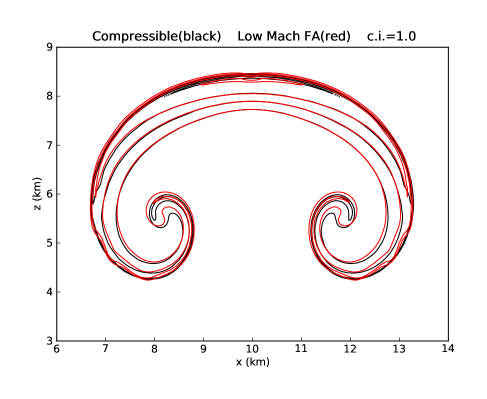
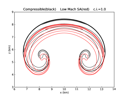
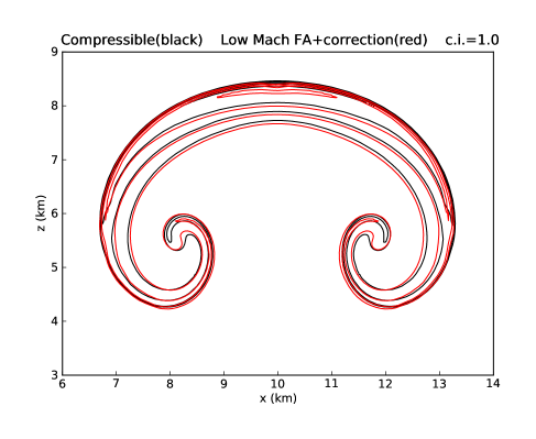
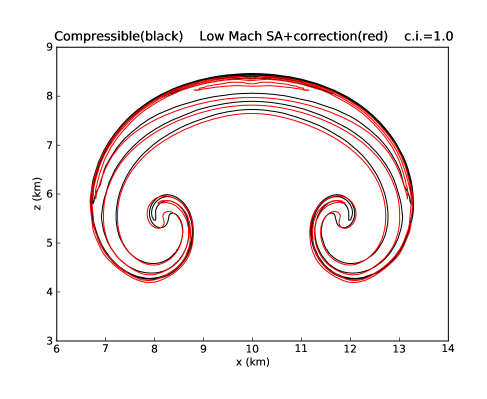
Figure 1: Comparison with the compressible solution for the moist thermal simulations at $1000\,$s. Perturbational potential temperature is shown with contours every $1\,$K: first (left) and second approach (right) The simulations in the bottom row include the $\delta\Gamma_{1}$–correction.

Figure 1 shows results from computations of the problem described above; in this figure $\theta^{\prime}_{e}$ from the low Mach number simulations is overlaid on the reference compressible solution, which was computed with the fully coupled compressible solver described in [DAB⁺14] and validated against results from [BF02]. The low Mach number simulations were carried out on a uniform grid of $512\times 256$; the compressible solution was performed on a finer grid of $1024\times 512$ in order to get a more accurate reference solution. In the top row of Figure 1 we see that the low Mach number computation using the first approach agrees well with the compressible solution. The computation with the second approach, however, shows a significant height difference of the top of the thermal. In the bottom row of Figure 1 we see that accounting for the local variation of $\gamma_{m}(\boldsymbol{x})$ and $\widetilde{\gamma}_{m}(\boldsymbol{x})$ through the the $\delta\Gamma_{1}$–correction described in §4 improves the fidelity of both approaches. With the first approach we see the improvement mostly in the tips; with the second approach the height of the thermal is noticeably improved. The fact that including the $\delta\Gamma_{1}$–correction impacts the second approach more dramatically than the first is consistent with the observation that replacing $\gamma_{m}(\boldsymbol{x})$ by $\overline{\gamma}_{m}$ in the first approach meant neglecting local variations in $\gamma_{m}(\boldsymbol{x})$ from $-8\times 10^{-5}$ to $6.5\times 10^{-4}$, while replacing $\widetilde{\gamma}_{m}(\boldsymbol{x})$ by $\overline{\widetilde{\gamma}}_{m}$ in the second approach meant neglecting local variations in $\widetilde{\gamma}_{m}(\boldsymbol{x})$ at least an order of magnitude larger, i.e. from $-6.7\times 10^{-3}$ to $1.5\times 10^{-3}.$ This behavior follows naturally from the fact that in the modified divergence constraint (eq. (31)), $\widetilde{\gamma}_{m}(\boldsymbol{x})$ accounts not only for the varying water composition but also for all the latent heat released during phase transitions (see Appendix C); therefore, local variations in $\widetilde{\gamma}_{m}(\boldsymbol{x})$ are expected to be more important.

The formalism adopted for the present low Mach model considers straightforwardly the effects of the specific heats of liquid water and water vapor in the evaluation of the thermodynamic properties of the moist fluid, and in particular in the definition of the internal energy and specific enthalpy of moist air, (8) and (9). The latter is not possible within the moist pseudo-incompressible model introduced in [OK14], which relies on a $\theta-\pi$ (potential temperature – Exner pressure) formalism defined with the specific heat of dry air. Neglecting the specific heats of liquid water and water vapor in our model amounts to consider the Equation set A investigated in [BF02] for the same isentropic background configuration. This is also the benchmark problem considered in [OK14] to validate their model. Figure 2 shows the low Mach number solution when the specific heats of water are neglected and contrasts it to the general case where all specific heats are taken into account, like in Figure 1. In [BF02], the maximum and minimum values for $\theta^{\prime}_{e}$ are $2.13647\,$K and $-1.39627\,$K, respectively. As discussed in [BF02], the impact of approximating thermodynamic properties of moist air can lead to important variations for certain configurations, as illustrated in this example.

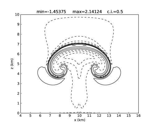
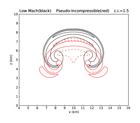
Figure 2: Solution to the isentropic background problem neglecting the specific heats of liquid water and vapor water. Left: perturbational potential temperature shown with contours every $0.5\,$K; negative contours are dashed. Contrast to Fig. 6(a) in [BF02]. Right: comparison with the low Mach number solution shown in Figure 1 (bottom left); perturbational potential temperature is shown with contours every $1.5\,$K.

5.2 Non–isentropic background state

We next consider a non–isentropic background state given by the hydrostatically balanced profiles in [CF84] (eq. 2). For the following computations we define a computational domain $4\,$km high and wide, with periodic horizontal boundary conditions. The boundary conditions at the top and bottom boundaries are as described for the isentropic case, except for the thermodynamic variables which are extrapolated to determine the corresponding fluxes. Again we use the configuration and parameters as given in [DAB⁺14]. All simulations with the low Mach formulation were performed on a uniform grid of $256\times 256$. As before, the reference compressible solutions were computed on a finer grid, here $1024\times 1024$.

The initial distributions of water vapor and liquid water in the atmosphere are set by the relative humidity in the atmosphere, RH, measured in percentage and defined as RH$~{}=(p_{v}/p_{v}^{*})\times 100$. In particular if RH${}_{0}<100\,$%, then no liquid water should be initially present in the atmosphere in order to guarantee the thermodynamic equilibrium of the initial state. Following [DAB⁺14], we consider in this study two cases: first, a saturated medium with RH${}_{0}=100\,$% and $q_{l}>0$ everywhere in the domain as in the isentropic background problem; and a second configuration with RH${}_{0}=20\,$%, and hence, no liquid water in the initial background state.

Let us consider the first configuration with an initially saturated environment. As described in [DAB⁺14], we initially introduce a warm perturbation of temperature. Figure 3 shows solutions obtained with the low Mach formulation using the first and second approach for the divergence constraint, as well as the compressible reference solution. Solutions are very similar in all three cases even though the low Mach approximations yield thermals rising slightly faster. In contrast to the previous example, introducing the $\delta\Gamma_{1}$–correction does not visibly change the results. For a $256\times 256$ grid and a CFL factor of $0.9$, the time steps for the low Mach approximations are about $1.4\,$s compared to $0.04\,$s with the compressible formulation. The low Mach number simulation takes roughly a factor of $13$ less computational time than the compressible simulation.

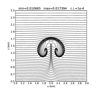
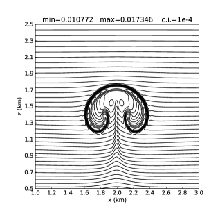
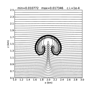
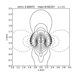
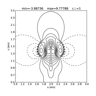
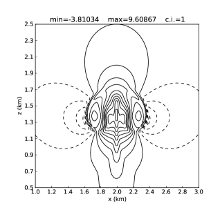
Figure 3: Initially saturated, non–isentropic background state. Liquid water mass fraction (top) and vertical velocity (bottom) are shown for the reference compressible (left), and low Mach number solution at $300\,$s using the first (center) and second (right) approach. Contours are every $10^{-4}$ (top) and $1\,$m s^-1 (bottom); negative contours are dashed.

For the second configuration with RH${}_{0}=20\,$%, we consider the same previous temperature perturbation and an additional circular perturbation in the relative humidity, which is set to $100\,$%, with a transition layer, as detailed in [DAB⁺14]. Initially there is no liquid water in the domain. Like Figure 1, Figure 4 compares the two low Mach number solutions to the reference compressible solution; the top row shows the results using laterally averaged $\gamma_{m}$ and $\widetilde{\gamma}_{m},$ while the bottom row shows the results using the $\delta\Gamma_{1}$–correction. Here the deviation of $\gamma_{m}(\boldsymbol{x})$ from $\overline{\gamma}_{m}(z)$ in the first approach ranges from $-4.2\times 10^{-3}$ to $6.9\times 10^{-4},$ which is considerably smaller than the deviation of $\widetilde{\gamma}_{m}(\boldsymbol{x})$ from $\overline{\widetilde{\gamma}}_{m}(z)$ in the second approach, which ranges from $-0.17$ to $3.3\times 10^{-2}$.

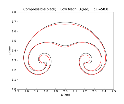
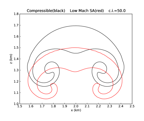
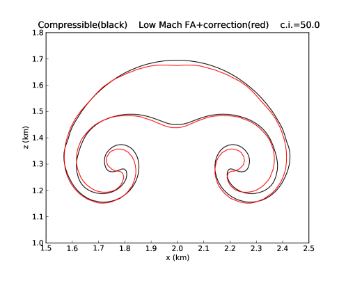
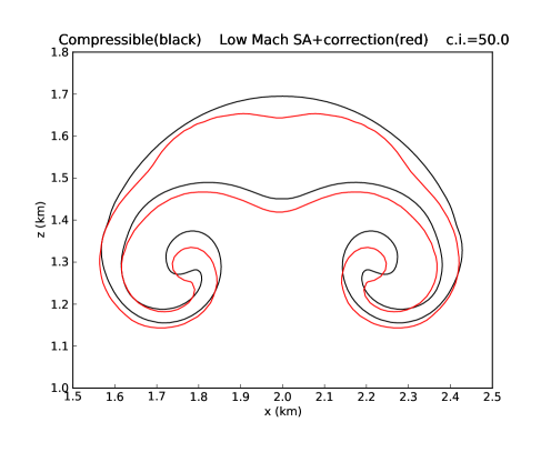
Figure 4: Non–isentropic background state with a saturated perturbation. Moist specific entropy is shown with contours every $50\,$J kg^-1 K^-1. The low Mach number solution at $300\,$s (red) using the first (left) and second (right) approach overlays the reference compressible solution (black). On the bottom are simulations that use the $\delta\Gamma_{1}$–correction.

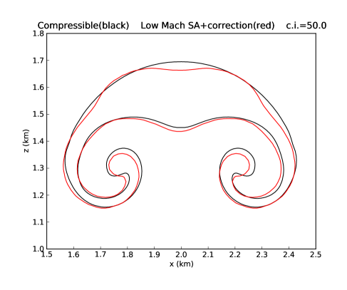
Figure 5: Non–isentropic background state with a saturated perturbation. Moist specific entropy is shown with contours every $50\,$J kg^-1 K^-1. The low Mach solution at $300\,$s (red) using the $\delta\Gamma_{1}$–correction given by (38) overlays the reference compressible solution (black).

Better agreement can be seen in Figure 5, where a term of order $\delta\Gamma_{1}^{2}$ is also considered in (36) for the $\delta\Gamma_{1}$–correction:

$$\boldsymbol{\nabla}\boldsymbol{\cdot}\boldsymbol{U}=-\frac{1}{\overline{\Gamma}_{1}p_{0}}\frac{Dp_{0}}{Dt}+S+\frac{\delta\Gamma_{1}}{\overline{\Gamma}_{1}^{2}p_{0}}\frac{Dp_{0}}{Dt}-\frac{\delta\Gamma_{1}^{2}}{\overline{\Gamma}_{1}^{3}p_{0}}\frac{Dp_{0}}{Dt}.$$ (38)

The time steps used in the low Mach computations are about $2.1\,$s, compared to $0.04\,$s with the compressible formulation. The low Mach number simulation takes roughly a factor of $15$ less computational time than the compressible simulation.

5.3 Three–dimensional simulation

Finally, we consider two interacting thermals rising in a three–dimensional, non–isentropically stratified background in a domain $10\,$km on a side and $15\,$km high. The background state is defined as in §5.2, with a relative humidity of RH${}_{0}=20\,$% and no liquid water in the initial configuration. The following temperature perturbation is then introduced:

$$T^{\prime}=6\cos^{2}\left(\frac{\pi L_{1}}{2}\right)+6\cos^{2}\left(\frac{\pi L_{2}}{2}\right),$$

where $L_{1}=\min(1,r_{1}),\;\;L_{2}=\min(1,r_{2}),$ and

$$r_{1}=\frac{1}{4}\sqrt{\left({x-x_{1}}\right)^{2}+\left({y-y_{1}}\right)^{2}+\left({z-z_{1}}\right)^{2}}\;,$$

$$r_{2}=\frac{1}{3}\sqrt{\left({x-x_{2}}\right)^{2}+\left({y-y_{2}}\right)^{2}+\left({z-z_{2}}\right)^{2}},$$

with $x_{1}=y_{1}=5\,$km, $z_{1}=7.5\,$km and $x_{2}=y_{2}=7\,$km, $z_{2}=7.5\,$km. Within the regions where the temperature is perturbed, we also perturb the relative humidity by setting RH equal to $50\,$% for $r_{1}<3\,$km and $r_{2}<2\,$km, for each initial thermal, with corresponding transition layers:

$${\rm RH}={\rm RH}_{0}+(50-{\rm RH}_{0})\cos^{2}\left(\frac{\pi}{2}\left[r_{1}-3\right]\right),\ 3\leq r_{1}\leq 4,$$

$${\rm RH}={\rm RH}_{0}+(50-{\rm RH}_{0})\cos^{2}\left(\frac{\pi}{2}\left[r_{2}-2\right]\right),\ 2\leq r_{2}\leq 3.$$

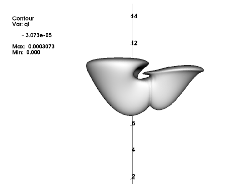
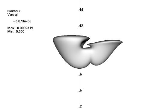
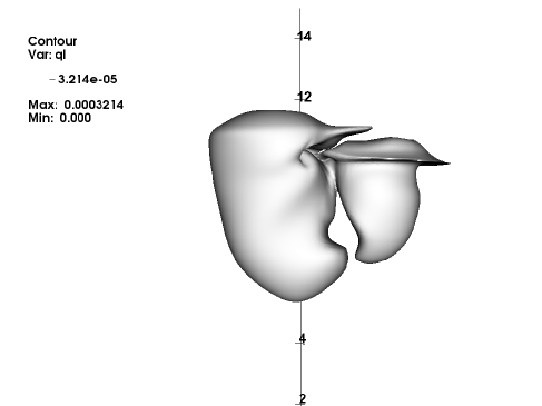
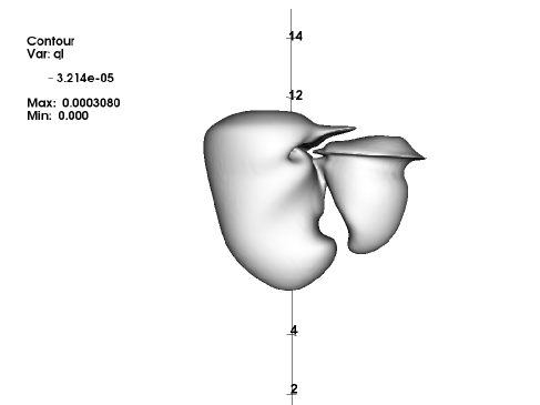
Figure 6: Two interacting thermals in a three–dimensional non–isentropic background state. Isosurfaces of liquid water for the reference compressible solutions (left) and the low Mach number ones (right) at times $500\,$s ($q_{l}=3.073\times 10^{-5}$) (top) and $1000\,$s (bottom) ($q_{l}=3.214\times 10^{-5}$). The low Mach number solver uses the modified divergence constraint (31) (second approach) with the $\delta\Gamma_{1}$–correction given by (38).

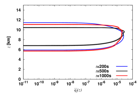
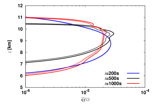
Figure 7: Horizontal budgets of liquid water, $\overline{q_{l}}(z)$, computed with (33) at $t=200\,$s, $500\,$s and $1000\,$s. Reference compressible and low Mach number solutions are represented with solid and dashed lines, respectively. More details can be appreciated in the zoomed region (right).

We consider the low Mach number formalism using the second approach (modified divergence constraint (31)) to numerically implement phase transitions, with the $\delta\Gamma_{1}$–correction given by (38). As before, the low Mach number solutions are contrasted to reference compressible solutions. For a uniform grid of size $256\times 256\times 384$, the time step in the low Mach number simulation is approximately $3\,$s, compared to $0.1\,$s in the compressible simulation. For this particular problem, the total run time of the low Mach number simulation is roughly a factor of $5$ less than that of the compressible simulation. Figure 6 illustrates the formation of liquid water as computed with both formulations. The relative difference between the maximum values of $q_{l}$ in the compressible and the low Mach number solutions is roughly $8\,$% at $t=500\,$s and $4\,$% at $t=1000\,$s, the two times shown in Figure 6. Figure 7 shows the horizontal budgets of liquid water, $\overline{q_{l}}(z)$, computed using formula (33), at $t=200$s and at the two simulation times shown in Figure 6. For $t=200\,$s practically the same solution is recovered with both formulations, with a relative difference of $0.2\,$% between the maximum values of $q_{l}$. Recalling that $q_{l}$ is diagnostically recovered in both the compressible and the low Mach number approach, we can track the formation of liquid water by computing it after each time step for comparison purposes. Local values of $q_{l}$ larger than $10^{-10}$ appear after $111\,$s and $112.5\,$s for the compressible and low Mach number simulations, respectively. The Mach number $M$ associated with this particular problem remains lower than $0.05$ during the entire numerical simulation.

6 Summary

We have presented a new low Mach number model for moist atmospheric flows with a general equation of state, based on the low Mach number model for stratified reacting flows introduced in [ABNZ08]. In our model we consider only reversible processes, namely water phase changes as in [OK14], using an exact Clausius–Clapeyron formula for moist thermodynamics and considering the effects of the specific heats of water and the temperature dependency of the latent heat. A set of invariant variables was used as prognostic variables in the equations of motion, including in particular the total water content and a specific enthalpy of moist air that accounts for the contribution of both sensible and latent heats. The evolution equations can thus be solved without needing to estimate or neglect source terms related to phase change during the time integration. The mass fractions of water vapor and liquid water are diagnostically recovered as required during a time step by imposing the saturation requirements of an atmosphere at thermodynamic equilibrium. The latter is an important property since updating the solution while ignoring the varying water composition, may negatively impact the accuracy of the moist flow dynamics, as investigated in [DAB⁺14].

We then considered a moist thermodynamic model that treats dry air and water vapor as ideal gases to define the equation of state for moist air. In order to account for the latent heat release in the low Mach divergence constraint for the velocity field, the evaporation rate is estimated from the time variation of saturated water vapor within a parcel. The amount of saturated water vapor within a parcel is determined by the Clausius–Clapeyron formula as a function of the local thermodynamical state; the evolution of the state depends on the local advected motions. An analytical expression for the evaporation rate was thus derived that depends on local parameters given by the temperature and pressure, the water composition, and the velocity field. Two approaches were then considered. In the first, the rate of phase change can be computed to evaluate the latent heat release; in the second, a modified divergence constraint can be analytically deduced by introducing the derived expression for the evaporation rate in the original divergence constraint. Both approaches are analytically equivalent and together with the low Mach number equation set allow us to characterize moist atmospheric flows.

The MAESTRO code [NAB⁺10], originally designed to simulate stratified reacting flows arising in astrophysical settings, was adapted to model moist atmospheric flows. A series of test problems was investigated with both isentropic and non–isentropic background states, as well as saturated and partially saturated regions in the atmosphere. Results were contrasted to reference solutions obtained with a fully compressible formulation. Very good agreement with the reference moist dynamics was shown using both the first and second approach (with the $\delta\Gamma_{1}$–correction), thus demonstrating that low Mach number models can serve as a reasonably accurate and computationally efficient alternative to compressible codes for small-scale moist atmospheric applications.

Appendix A Derivation of the low Mach divergence constraint

We rewrite the conservation of mass (eq. (1)) as an expression for the divergence of velocity,

$$\boldsymbol{\nabla}\boldsymbol{\cdot}\boldsymbol{U}=-\frac{1}{\rho}\frac{D\rho}{Dt}.$$ (39)

Differentiating the equation of state, written as $p=p(\rho,T,q_{a},q_{v},q_{l})$, along particle paths, we obtain

$$\frac{D\rho}{Dt} =\frac{1}{p_{\rho}}\left(\frac{Dp}{Dt}-p_{T}\frac{DT}{Dt}-\sum_{i\in(a,v,l)}p_{q_{i}}\frac{Dq_{i}}{Dt}\right)$$

$$=\frac{1}{p_{\rho}}\left(\frac{Dp}{Dt}-p_{T}\frac{DT}{Dt}-\left(p_{q_{v}}-p_{q_{l}}\right)\frac{e_{v}}{\rho}\right),$$

with $p_{\rho}=\partial p/\partial\rho|_{T,q_{i}}$, $p_{T}=\partial p/\partial T|_{\rho,q_{i}}$, and $p_{q_{i}}=\partial p/\partial q_{i}|_{\rho,T,(q_{j},j\neq i)}$. An expression for $DT/Dt$ can be obtained by differentiating the definition of moist enthalpy (eq. (9)), and comparing terms with the enthalpy equation (3):

$$\rho\frac{D\widehat{h}}{Dt} =\rho\left(\left.\frac{\partial\widehat{h}}{\partial T}\right|_{p,q_{i}}\frac{DT}{Dt}+\left.\frac{\partial\widehat{h}}{\partial p}\right|_{T,q_{i}}\frac{Dp}{Dt}+\sum_{i\in(a,v,l)}\left.\frac{\partial\widehat{h}}{\partial q_{i}}\right|_{T,p,(q_{j},j\neq i)}\frac{Dq_{i}}{Dt}\right)$$

$$=\rho\left(c_{pm}\frac{DT}{Dt}+\widehat{h}_{p}\frac{Dp}{Dt}+\left(\widehat{h}_{q_{v}}-\widehat{h}_{q_{l}}\right)\frac{e_{v}}{\rho}\right)$$

$$=\frac{Dp}{Dt}+\rho\mathcal{H},$$

or, gathering terms,

$$\frac{DT}{Dt}=\frac{1}{\rho c_{pm}}\left[\left(1-\rho\widehat{h}_{p}\right)\frac{Dp}{Dt}-\left(\widehat{h}_{q_{v}}-\widehat{h}_{q_{l}}\right)e_{v}+\rho\mathcal{H}\right],$$ (40)

where $c_{pm}=\partial\widehat{h}/\partial T|_{p,q_{i}}$ is the specific heat of moist air at constant pressure, $\widehat{h}_{p}=\partial\widehat{h}/\partial p|_{T,q_{i}}$, and $\widehat{h}_{q_{i}}=\partial\widehat{h}/\partial q_{i}|_{T,p,(q_{j},j\neq i)}$. Coming back to equation (39) and replacing $p$ by $p_{0}(z,t)$, we can write the divergence constraint on the velocity field as (12) with $\alpha$ and $S$ given by (13).

Appendix B Derivation of the evaporation rate

Considering that $e_{v}=\rho Dq_{v}^{*}/Dt$ from (28) and differentiating $q_{v}^{*}=q_{v}^{*}(\rho,T)$ (eq. (25)) along particle paths, we obtain

$$e_{v}=\rho\left[\left.\frac{\partial q_{v}^{*}}{\partial\rho}\right|_{T}\frac{D\rho}{Dt}+\left.\frac{\partial q_{v}^{*}}{\partial T}\right|_{\rho}\frac{DT}{Dt}\right],$$

with

$$\left.\frac{\partial q_{v}^{*}}{\partial\rho}\right|_{T}=-\frac{q_{v}^{*}}{\rho},\qquad\left.\frac{\partial q_{v}^{*}}{\partial T}\right|_{\rho}=q_{v}^{*}\left(\frac{\alpha_{v}-1}{T}+\frac{\beta_{v}}{{T}^{2}}\right)=q_{v}^{*}\phi(T),$$

according to (25) and (23). With the equation of state (20), equation (40) becomes

$$\frac{DT}{Dt}=\frac{1}{\rho c_{pm}}\left[\frac{Dp}{Dt}-L_{e}e_{v}+\rho\mathcal{H}\right],$$ (41)

and hence,

$$e_{v}=\frac{q_{v}^{*}\left[\rho c_{pm}\left(\boldsymbol{\nabla}\boldsymbol{\cdot}\boldsymbol{U}\right)+\phi(T)\displaystyle\left(\frac{Dp}{Dt}+\rho\mathcal{H}\right)\right]}{c_{pm}+q_{v}^{*}\phi(T)L_{e}};$$ (42)

that is,

$${\mathcal{A}}_{e}=\frac{q_{v}^{*}\rho c_{pm}}{c_{pm}+q_{v}^{*}\phi(T)L_{e}},\qquad{\mathcal{B}}_{e}=\frac{q_{v}^{*}\phi(T)}{c_{pm}+q_{v}^{*}\phi(T)L_{e}},\qquad{\mathcal{C}}_{e}=\frac{q_{v}^{*}\phi(T)}{c_{pm}+q_{v}^{*}\phi(T)L_{e}},$$ (43)

into (29), replacing also $p$ by $p_{0}(z,t)$.

Notice that another expression for $e_{v}$ can be derived considering $q_{v}^{*}=q_{v}^{*}(q_{a},p,T)$ (eq. (26)) in $e_{v}=\rho Dq_{v}^{*}/Dt$. Moreover, two more expressions for $e_{v}$ can be found using

$$\frac{DT}{Dt}=\frac{1}{\rho c_{vm}}\left[-p\left(\boldsymbol{\nabla}\boldsymbol{\cdot}\boldsymbol{U}\right)-(L_{e}-R_{v}T)e_{v}+\rho\mathcal{H}\right],$$

instead of (41), deduced from the conservation equation for internal energy $\widehat{e}$ instead of enthalpy $\widehat{h}$. Numerical computations using different formulations for $e_{v}$ yield practically identical results.

Appendix C Modified divergence constraint

Rearranging terms in (30), after having introduced the estimate of $e_{v}$ (eq. (29)) in $S$ (eq. (21)), yields the modified divergence constraint (31) with

$$\widetilde{\alpha}=\displaystyle\frac{\displaystyle\frac{1}{\gamma_{m}p_{0}}-\frac{{\mathcal{B}}_{e}}{\rho}\left[\frac{1}{(\epsilon q_{a}+q_{v})}-\frac{L_{e}}{c_{pm}T}\right]}{1-\displaystyle\frac{{\mathcal{A}}_{e}}{\rho}\left[\frac{1}{(\epsilon q_{a}+q_{v})}-\frac{L_{e}}{c_{pm}T}\right]},$$

$$\widetilde{S}=\displaystyle\frac{\displaystyle\left[\frac{1}{c_{pm}T}\right]\mathcal{H}+{\mathcal{C}}_{e}\left[\frac{1}{(\epsilon q_{a}+q_{v})}-\frac{L_{e}}{c_{pm}T}\right]\mathcal{H}}{1-\displaystyle\frac{{\mathcal{A}}_{e}}{\rho}\left[\frac{1}{(\epsilon q_{a}+q_{v})}-\frac{L_{e}}{c_{pm}T}\right]}=\widetilde{\sigma}\mathcal{H};$$

and thus

$$\widetilde{\sigma}=\frac{\rho\left\{(\epsilon q_{a}+q_{v})+{\mathcal{C}}_{e}\left[c_{pm}T-(\epsilon q_{a}+q_{v})L_{e}\right]\right\}}{(\epsilon q_{a}+q_{v})\rho c_{pm}T-{\mathcal{A}}_{e}\left[c_{pm}T-(\epsilon q_{a}+q_{v})L_{e}\right]}.$$ (44)

After some manipulation, we can write that $\widetilde{\alpha}=1/(\widetilde{\gamma}_{m}p_{0})$ with

$$\widetilde{\gamma}_{m}=\gamma_{m}\left[\displaystyle\frac{1+c_{vm}\varPhi}{1+R_{m}T\phi(T)\varPhi}\right],\qquad\varPhi=\displaystyle\frac{q_{v}^{*}\left[R_{m}L_{e}-c_{pm}R_{v}T\right]}{c_{vm}R_{m}T\left[c_{pm}+q_{v}^{*}\phi(T)L_{e}\right]},$$ (45)

using (43). In particular if there is no phase transition ($e_{v}=0$), then $\varPhi=0$ and $\widetilde{\gamma}_{m}=\gamma_{m}$; similarly, ${\mathcal{A}}_{e}={\mathcal{C}}_{e}=0$ in (44) and $\widetilde{\sigma}=\sigma$.

As pointed out in Appendix B, three more expressions for $e_{v}$, other than (42), can be derived yielding four different formulations for $\widetilde{\alpha}$ and $\widetilde{S}$ in the modified divergence constraint (31). Nevertheless, all of them yield practically identical numerical results.

References

- [ABNZ08] A. S. Almgren, J. B. Bell, A. Nonaka, and M. Zingale. Low Mach number modeling of Type Ia supernovae. III. Reactions. ApJ, 684:449–470, 2008.
- [ABNZ15] A. S. Almgren, J. B. Bell, A. Nonaka, and M. Zingale. On new low Mach number equations for stratified flows. In preparation, 2015.
- [ABRZ06a] A. S. Almgren, J. B. Bell, C. A. Rendleman, and M. Zingale. Low Mach number modeling of Type Ia supernovae. I. Hydrodynamics. ApJ, 637:922–936, 2006.
- [ABRZ06b] A. S. Almgren, J. B. Bell, C. A. Rendleman, and M. Zingale. Low Mach number modeling of Type Ia supernovae. II. Energy evolution. ApJ, 649:927–938, 2006.
- [Alm00] A. S. Almgren. A new look at the pseudo-incompressible solution to Lamb’s problem of hydrostatic adjustment. J. Atmos. Sci., 57:995–998, April 2000.
- [Bat53] G. K. Batchelor. The conditions for dynamical similarity of motions of a frictionless perfect-gas atmosphere. Q. J. R. Meteorol. Soc., 79:224–235, 1953.
- [Bet73] A. K. Betts. Non–precipitating cumulus convection and its parameterization. Q. J. R. Meteorol. Soc., 99(419):178–196, 1973.
- [BF02] G. H. Bryan and J. M. Fritsch. A benchmark simulation for moist nonhydrostatic numerical models. Mon. Wea. Rev., 130:2917–2928, 2002.
- [CF84] T. L. Clark and R. D. Farley. Severe downslope windstorm calculations in two and three spatial dimensions using anelastic interactive grid nesting: A possible mechanism for gustiness. J. Atmos. Sci., 41:329–350, 1984.
- [Cla79] T. L. Clark. Numerical simulations with a three-dimensional cloud model: Lateral boundary condition experiments and multicellular severe storm simulations. J. Atmos. Sci., 36:2191–2215, 1979.
- [DAB+14] M. Duarte, A. S. Almgren, K. Balakrishnan, J. B. Bell, and D. M. Romps. A numerical study of methods for moist atmospheric flows: Compressible equations. Mon. Wea. Rev., 142:4269–4283, 2014.
- [DF69] J. A. Dutton and G. H. Fichtl. Approximate equations of motion for gases and liquids. J. Atmos. Sci., 26:241–254, 1969.
- [Dur89] D. R. Durran. Improving the anelastic approximation. J. Atmos. Sci., 46(11):1453–1461, 1989.
- [GC91] W. W. Grabowski and T. L. Clark. Cloud-environment interface instability: Rising thermal calculations in two spatial dimensions. J. Atmos. Sci., 48:527–546, 1991.
- [Gou69] D. O. Gough. The anelastic approximation for thermal convection. J. Atmos. Sci., 26:448–456, 1969.
- [GS90] W. W. Grabowski and P. K. Smolarkiewicz. Monotone finite-difference approximations to the advection-condensation problem. Mon. Wea. Rev., 118:2082–2097, 1990.
- [GS02] W. W. Grabowski and P. K. Smolarkiewicz. A multiscale anelastic model for meteorological research. Mon. Wea. Rev., 130:939–956, 2002.
- [HH89] T. Hauf and H. Höller. Entropy and potential temperature. J. Atmos. Sci., 44:2887–2901, 1989.
- [Kle09] R. Klein. Asymptotics, structure, and integration of sound-proof atmospheric flow equations. Theor. Comput. Fluid Dyn., 23(3):161–195, 2009.
- [KP12] R. Klein and O. Pauluis. Thermodynamic consistency of a pseudoincompressible approximation for general equations of state. J. Atmos. Sci., 69:961–968, 2012.
- [KSD07] J. B. Klemp, W. C. Skamarock, and J. Dudhia. Conservative split-explicit time integration methods for the compressible nonhydrostatic equations. Mon. Wea. Rev., 135:2897–2913, 2007.
- [KW78] J. B. Klemp and R. B. Wilhelmson. The simulation of three-dimensional convective storm dynamics. J. Atmos. Sci., 35:1070–1096, 1978.
- [LH82] F. Lipps and R. Hemler. A scale analysis of deep moist convection and some related numerical calculations. J. Atmos. Sci., 39:2192–2210, 1982.
- [NAB+10] A. Nonaka, A. S. Almgren, J. B. Bell, M. J. Lijewski, C. Malone, and M. Zingale. MAESTRO: An adaptive low Mach number hydrodynamics algorithm for stellar flows. ApJS, 188:358–383, 2010.
- [OK14] W. P. O’Neill and R. Klein. A moist pseudo-incompressible model. Atmos. Res., 142:133–141, 2014.
- [Ooy90] K. V. Ooyama. A thermodynamic foundation for modeling the moist atmosphere. J. Atmos. Sci., 47:2580–2593, 1990.
- [OP62] Y. Ogura and N. A. Phillips. Scale analysis of deep and shallow convection in the atmosphere. J. Atmos. Sci., 19:173–179, 1962.
- [Rom08] D. M. Romps. The dry-entropy budget of a moist atmosphere. J. Atmos. Sci., 65:3779–3799, 2008.
- [Sat03] M. Satoh. Conservative scheme for a compressible nonhydrostatic model with moist processes. Mon. Wea. Rev., 131:1033–1050, 2003.
- [SO73] S.-T. Soong and Y. Ogura. A comparison between axisymmetric and slab-symmetric cumulus cloud models. J. Atmos. Sci., 30:879–893, 1973.
- [TC81] G. J. Tripoli and W. R. Cotton. The use of lce-liquid water potential temperature as a thermodynamic variable in deep atmospheric models. Mon. Wea. Rev., 109:1094–1102, 1981.
- [TW76] M. C. Tapp and P. W. White. A non-hydrostatic mesoscale model. Q. J. Roy. Meteor. Soc., 102(432):277–296, 1976.
- [VLB+13] G. M. Vasil, D. Lecoanet, B. P. Brown, T. S. Wood, and E. G. Zweibel. Energy conservation and gravity waves in sound-proof treatments of stellar interiors. II. Lagrangian constrained analysis. ApJ, 773(2):169, 2013.