Abstract

Contents

1. 1 Introduction
2. 2 Degenerations to $\mathbb{CP}(a^{2},b^{2},c^{2})$ and almost toric fibrations
3. 3 Neck Stretching - SFT
   1. 3.1 Splitting
   2. 3.2 Almost complex structures - compatible and adjusted
   3. 3.3 Example
   4. 3.4 Compactness Theorem
4. 4 Proof of Theorem 1.1
   1. 4.1 Preliminary results
   2. 4.2 The setup
   3. 4.3 The proof

1 Introduction

In [15], we explicitly constructed a monotone Lagrangian torus in $\mathbb{CP}^{2}$, which we named $T(1,4,25)$. Moreover, we computed the number of Maslov index 2 discs bounded by $T(1,4,25)$, to prove it is not Hamiltonian isotopic to the known Clifford and Chekanov tori.

An almost toric fibration is a singular Lagrangian torus fibration allowing nodal (pinched torus) and elliptic (circles or points) singularities; see Definition 2.9 of [15]. The $T(1,4,25)$ Lagrangian torus can be seen as the ‘central’ fiber of a particular almost toric fibration of $\mathbb{CP}^{2}$. This almost toric fibration can be obtained from the standard toric fibration of $\mathbb{CP}^{2}$ by a series of operations called nodal trades and nodal slides that don’t change the symplectic four manifold - see Definitions 2.12, 2.13 of [15]. Nodal trade replaces a corner (corank 2 elliptic singularity) by a nodal fiber in the interior of the fibration with a cut that encodes the monodromy around the nodal fiber. Nodal slides amount to lengthening and shortening the cut. The base diagram for the almost toric fibration containing the $T(1,4,25)$ monotone Lagrangian torus can be arranged to look similar to the base for the standard toric fibration of the orbifold weighted projective space $\mathbb{CP}(1,4,25)$, but with nodal fibers and cuts replacing the orbifold points - see Figure 1. Performing nodal slides that shorten all the cuts to a limit point, pushing the nodes all the way to the boundary, corresponds to a degeneration from $\mathbb{CP}^{2}$ to the weighted projective space $\mathbb{CP}(1,4,25)$. Following the degeneration, $T(1,4,25)$ goes to the ‘central’ fiber of the standard base diagram of $\mathbb{CP}(1,4,25)$.

The projective plane admits degenerations to weighted projective spaces $\mathbb{CP}(a^{2},b^{2},c^{2})$, where $(a,b,c)$ is a Markov triple, i. e., satisfies the Markov equation:

$$a^{2}+b^{2}+c^{2}=3abc.$$ (1.1)

For each $\mathbb{CP}(a^{2},b^{2},c^{2})$, one can associate a monotone Lagrangian torus, $T(a^{2},b^{2},c^{2})$, in $\mathbb{CP}^{2}$ in either of the following ways:

• by following the necessary nodal trade, nodal slide and transferring the cut - see Definition 2.1 - operations until we get to a base diagram that is about to degenerate to the base of the moment map for the standard torus action on $\mathbb{CP}(a^{2},b^{2},c^{2})$ and considering the monotone fiber - see section 2, Proposition 2.4;

• by performing three rational blowdown surgeries on $\mathbb{CP}(a^{2},b^{2},c^{2})$ - see section 10 of [14] - that replace a small neighbourhood of each point mapping to the vertex of the moment polytope of $\mathbb{CP}(a^{2},b^{2},c^{2})$, having a lens space of the form $L(k^{2},kl-1)$ as its boundary by a rational ball having the same boundary - see Figure 2 - and considering the monotone fiber.

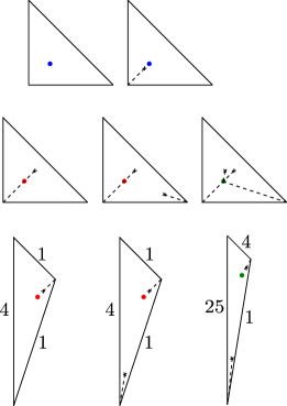
Figure 1: The procedure for going from the Clifford torus on the top left base diagram, to the Chekanov torus (third base diagram) and to the $T(1,4,25)$ torus (fifth base diagram) by applying nodal trades and nodal slides - see [15, 14, 12] for definitions. The dots represent the image of the monotone tori in the base diagrams. Each of the bottom diagrams is equivalent to the one right above it since they are related by transferring the cut operations - see Definition 2.1.

We will prove:

Theorem 1.1.

If $(a,b,c)$ and $(d,e,f)$ are two distinct Markov triples then the monotone Lagrangian tori $T(a^{2},b^{2},c^{2})$ and $T(d^{2},e^{2},f^{2})$ are not Hamiltonian isotopic.

In [15], we gave an explicit description of $T(1,4,25)$. We first predicted the number of Maslov index 2 discs each $T(1,4,25)$ bounds, by applying wall-crossing mutations to the superpotential, as described by Galkin and Usnich in [9] - see also sections 2.4 and 3 of [15]. But unfortunately wallcrossing formulas are not proved to hold yet. That forced us to directly compute all the Maslov index 2 holomorphic discs $T(1,4,25)$ bounds.

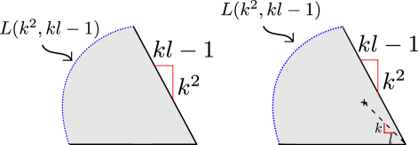
Figure 2: The picture on the left represents the base of a toric neighbourhood of an orbifold point. The picture on the right is the base of an almost toric fibration on a rational ball having the boundary the lens space $L(k^{2},kl-1)$. The lens space $L(k^{2},kl-1)$ is the union of the fibers over the dotted component of the boundary of the base diagrams.

In this paper, we employ the technique of neck-stretching from symplectic field theory. We use it to find restrictions on the relative homotopy classes in $\pi_{2}(\mathbb{CP}^{2},T(a^{2},b^{2},c^{2}))$ that can be represented by a holomorphic disc with Maslov index 2. More precisely, we describe the convex hull of all classes in $\pi_{2}(\mathbb{CP}^{2},$ $T(a^{2},b^{2},c^{2}))$, represented by Maslov index 2 holomorphic discs. It follows directly from the work of Gromov [11] that one can construct Hamiltonian isotopy invariants for monotone Lagrangian submanifolds from algebraic counts of holomorphic discs with Maslov index 2 (Theorem 6.4 of [15]). This is a well known fact in the symplectic geometry community and was inferred in Proposition 4.1.A of [8]. Using this invariants we are able to distinguish the tori $T(a^{2},b^{2},c^{2})$ for different Markov triples.

This is the first example of infinitely many Lagrangian isotopic but not Hamiltonian isotopic monotone Lagrangian tori living in a compact symplectic manifold. A similar result in $\mathbb{R}^{6}$ was given by Auroux in [1].

Remark 1.2.

In [16], Wu used neck-stretching technique to compute holomorphic discs bounded by his torus arising as a ‘central’ fiber from a semi-toric system on $\mathbb{CP}^{2}$. By the description of the Chekanov torus as $T(1,1,4)$ given in [15], it was suggestive to us that this torus is a different presentation of the Chekanov torus. A proof that Wu’s torus, among others, is a presentation of the Chekanov torus is given by Oakley and Usher in [13].

Remark 1.3.

While writing this paper the author learned that Galkin and Mikhalkin have independently obtained the same result - [10].

The paper is organized as follows.

In section 2 we show that the boundary of a neighbourhood of an orbifold point in $\mathbb{CP}(a^{2},b^{2},c^{2})$ is contactomorphic to a lens spaces of the form $L(k^{2},kl-1)$ as their boundaries. Hence we can apply rational blowdown on these neighbourhoods, as in section 10 of [14]. We show that, after applying the rational blowdowns, we obtain an almost toric fibration of $\mathbb{CP}^{2}$. This is done by showing that we can get to the same almost toric fibration by performing a series of nodal trade, nodal slide and transferring the cut operations to the standard moment polytope of $\mathbb{CP}^{2}$.

In section 3 we describe a technique originating in symplectic field theory, often called neck-stretching. In the subsection 3.1, we give a quick review of neck-stretching, also known as splitting of a symplectic manifold along a contact hypersurface - see [7], [3], [16]. In subsection 3.2, we define what kind of almost complex structures are adjusted for the neck-stretching we perform. In section 3.3, we work out an example of neck-stretching that is important for the proof of Theorem 1.1. In subsection 3.4, we state, from [3] and [7], the main compactness theorem of pseudo-holomorphic curves for neck-stretching.

Section 4 is devoted to the proof of Theorem 1.1. We use the technique of neck- stretching to describe the convex hull of all classes in $\pi_{2}(\mathbb{CP}^{2},$ $T(a^{2},b^{2},c^{2}))$, represented by Maslov index 2 holomorphic discs. The proof then follows from Theorem 6.4 of [15] (Lemma 4.1), which is an immediate consequence of the work of Gromov [11] - see also proposition 4.1 A of [8].

Acknowledgments. I am extremely grateful to Denis Auroux for huge support and invaluable discussions. Also, I want to thank Weiwei Wu for useful discussions during my visit to Michigan State University. This work was supported by the CNPq - Conselho Nacional de Desenvolvimento Científico e Tecnológico, Ministry of Science, Technology and Innovation, Brazil; the Department of Mathematics of University of California at Berkeley; the National Science Foundation grant number DMS-1264662; and (during the revision of the paper) the Herchel Smith Postdoctoral Fellowship - Dep. of Pure Mathematics and Mathematical Statistics - University of Cambridge.

2 Degenerations to $\mathbb{CP}(a^{2},b^{2},c^{2})$ and almost toric fibrations

In this section, we show that, for each Markov triple $(a,b,c)$, there is a monotone Lagrangian torus $T(a^{2},b^{2},c^{2})$, which is the ‘barycentric fiber’ depicted in a base diagram of an almost toric fibration. For a detailed account on almost toric fibrations we refer the reader to the work of Symington [14] and Leung-Symington [12].

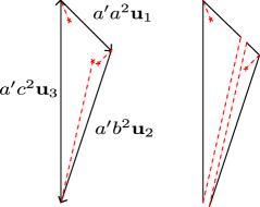
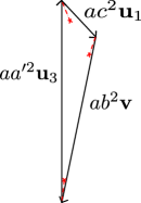
Figure 5: Transferring the cut operation to the left of the cut $R^{+}$. We multiplied by a factor of $a^{\prime}$ to simplify computations and lengthened the cut so that the resulting diagram contains $T(c^{2},b^{2},a^{\prime 2})$ as its barycentric fiber.

First, we will define an operation we call transferring the cut (Definition 2.1). A vector $v$ in a lattice $\Lambda$ is called a primitive vector, if it is not a positive multiple of another vector in the lattice. If $w=\lambda v\in\Lambda\otimes\mathbb{R}$, with $v\in\Lambda$ primitive and $\lambda\in\mathbb{R}_{\geq 0}$, we say that $w$ has affine length $\lambda$. Transferring the cut operation changes a base diagram in $\mathbb{R}^{2}$, whose edges have affine lengths $a^{2},b^{2},c^{2}$, into another base diagram whose edges have affine lengths $(3bc-a)^{2},b^{2},c^{2}$ (Proposition 2.4). These will represent the same almost toric fibration of $\mathbb{CP}^{2}$ (see Figure 5).

We recall that Markov triples are obtained from (1,1,1) by a sequence of ‘mutations’ of the form

$$(a,b,c)\rightarrow(a^{\prime}=3bc-a,b,c).$$ (2.1)

Hence, we show the claim of [15] that an almost toric fibration having $T(a^{2},b^{2},c^{2})$ as its central fiber can be obtained from the moment polytope of the standard torus action on $\mathbb{CP}^{2}$ by a series of nodal trade, nodal slide and transferring the cut operations.

Along the way, we show that the boundary of a neighbourhood of an orbifold point in $\mathbb{CP}(a^{2},b^{2},c^{2})$ is a lens space of the form $L(k^{2},kl-1)$. It follows then that we obtain an almost toric fibration of $\mathbb{CP}^{2}$ with $T(a^{2},b^{2},c^{2})$ as the central fiber by performing three rational blowdown operations on small neighbourhoods of the corners of the standard base diagram of $\mathbb{CP}(a^{2},b^{2},c^{2})$ - see section 10 of [14] and Figure 2.

Following the notation of section 5 of [14], let $(B,\mathcal{A},S)$ be a almost toric base of some almost toric fibration, where $B$ is the base of the singular Lagrangian fibration, $\mathcal{A}$ is the induced affine structure, $S=\bigcup_{i=1}^{N}\{s_{i}\}$ and $s_{i}\in B$ are the nodes. Denote by $\mathcal{A}_{0}$ the standard affine structure in $\mathbb{R}^{2}$. Recall that, for $b$ close to a node $s_{i}$, there is an eigendirection in $T_{b}B$ invariant under a monodromy around each $s_{i}$. An eigenline through $s_{i}$, is the maximal affine linear immersed one manifold tangent to eigendirection of $s_{i}$ at each $T_{b}B$. An eigenray is one of the two components of an eigenline minus the respective node. See definition 4.11 of [14].

Consider a base diagram $\Delta\subset\mathbb{R}^{2}$ (assume it is connected), which is the image of an affine embedding $\Phi$ of $(B\setminus\bigcup_{i=1}^{N}R_{i},\mathcal{A})$ into $(\mathbb{R}^{2},\mathcal{A}_{0})$, where $R_{i}$ is an (oriented) eigenray leaving the node $s_{i}$. Denote $R_{1}$ by $R^{+}$, the eigenline containing $R^{+}$ by $L$, and by $R^{-}\subset L$ the eigenray opposite to $R^{+}$. Let $P^{\pm}=\{\lim_{x\to y}\Phi(x)|x\in B;y\in R^{\pm}\}$, be the branch locus of $R^{\pm}$. We have that the branch locus of $L$, $P^{+}\cup\{s_{1}\}\cup P^{-}$, divides the base diagram $\Delta$ into two components, $\Delta_{l}$ (left) and $\Delta_{r}$ (right).

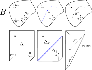
Figure 3: The top three pictures represents a base $B$ of an almost toric fibration with different set of eigenrays, represented by the dashed lines. Each one of the bottom three pictures is the image of an affine embedding of $B$ minus some eigenrays (the ones represented on the picture right above) into $\mathbb{R}^{2}$. By applying transferring the cut operation on the left of $R^{+}$ to the base diagram $\Delta$ (bottom left picture), we obtain the base diagram $\Delta^{\prime}$ (bottom right picture, after rescaling for visual purpose).

We will construct a new base diagram $\Delta^{\prime}$, corresponding to an affine embedding $\Phi^{\prime}$ of $(B\setminus R^{-}\cup\bigcup_{i=2}^{N}R_{i},\mathcal{A})$ into $(\mathbb{R}^{2},\mathcal{A}_{0})$, representing the same almost toric fibration as $\Delta$. Let $M^{lr}$ be the monodromy used to go from $\Delta_{l}$ to $\Delta_{r}$, through $P^{+}$. Essentially, $\Delta^{\prime}$ is obtained by gluing at $P^{+}$, $M^{lr}(\Delta_{l})$ to $\Delta_{r}$ , where the monodromy $M^{lr}$ is applied centred at $s_{1}$. In other words, $\Phi^{\prime}$ is equal to $\Phi$ on $\Phi^{-1}(\Delta_{r})$, to $M^{lr}\circ\Phi$ on $\Phi^{-1}(\Delta_{l})$ and extends continuously to $R^{+}$, so that $\Phi^{\prime}(R^{+})=P^{+}$.

Definition 2.1.

The base diagram $\Delta^{\prime}$ constructed above is said to be obtained from $\Delta$ by a transferring the cut operation on the left of $R^{+}$.

The definition of transferring the cut operation on the right of $R_{1}$ is obtained in a totally analogous way. From now on, we will abuse notation, as we also denote by $R^{+}$ its branched cover $P^{+}$.

Consider now the standard moment polytope of $\mathbb{CP}(a^{2},b^{2},c^{2})$, for $(a,b,c)$ Markov triple, with oriented edges $a^{2}\textbf{u}_{1}$, $b^{2}\textbf{u}_{2}$, $c^{2}\textbf{u}_{3}$, as in the left picture of Figure 4. We can arrange $\textbf{u}_{1}=(b^{2},-m_{1})$, $\textbf{u}_{2}=-(a^{2},m_{2})$, $\textbf{u}_{3}=(0,1)$.

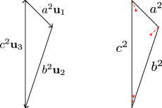
Figure 4: The left picture is the moment polytope for the standard torus action on $\mathbb{CP}(a^{2},b^{2},c^{2})$. The right picture is obtained form the left one by three rational blowdown operations on the neighbourhood of each vertex.

Proposition 2.2.

The positive integers $m_{1}$, $m_{2}$ are of the form $bl_{1}-1$, $al_{2}-1$, respectively, $l_{1},l_{2}$ in $\mathbb{Z}_{>0}$. Hence, the boundary of a neighbourhood of the vertex opposite to $a^{2}\textbf{u}_{1}$, respectively $b^{2}\textbf{u}_{2}$, is a lens space of the form $L(a^{2},al_{2}-1)$, respectively $L(b^{2},bl_{1}-1)$.

Proof.

First we note that $(a,b,c)$ are mutually co-prime. In fact, if $p$ divides two of them, by the Markov equation (1.1), it must divide the third one. The numbers $a^{\prime}=3bc-a$, $b^{\prime}=3ac-b$ and $c^{\prime}=3ab-c$ are also divisible by $p$. Since we can reduce any Markov triple to $(1,1,1)$ by applying mutations of the form (2.1), we must have $p=1$.

By equating the last coordinate of $a^{2}\textbf{u}_{1}+b^{2}\textbf{u}_{2}+c^{2}\textbf{u}_{3}=0$ and using the Markov relation (1.1) we get

$$a^{2}m_{1}+b^{2}m_{2} = c^{2},$$ (2.2)

$$a^{2}(m_{1}+1)+b^{2}(m_{2}+1) = 3abc.$$ (2.3)

Working modulo $a$ and modulo $b$, we must have $m_{1}=bl_{1}-1$, $m_{2}=al_{2}-1$. Positivity of $l_{1},l_{2}$ follows from positivity of $m_{1},m_{2}$.

The second statement of the Proposition follows immediately from section 9.3 of [14].

∎

By applying an appropriate $SL(2,\mathbb{Z})$ transformation to the base diagram, sending $\textbf{u}_{2}$ to $(0,1)$, allow us to conclude, using the above Proposition, that the remaining vertex has a neighbourhood with boundary a lens space of the form $L(c^{2},cl_{3}-1)$. Hence, we can apply rational blowdown operations in a neighbourhood of each vertex. We get from $\mathbb{CP}(a^{2},b^{2},c^{2})$, represented by its standard moment polytope, to the almost toric fibration represented by the right picture of Figure 4.

Remark 2.3.

Consider the primitive vectors $\textbf{w}_{1}=-(a,l_{2})$, $\textbf{w}_{2}=(-b,l_{1})$ and $\textbf{w}_{3}$ representing the cuts respectively opposite to the edges $a^{2}\textbf{u}_{1}$, $b^{2}\textbf{u}_{2}$, $c^{2}\textbf{u}_{3}$. The reader can verify that

$$\frac{ac\textbf{w}_{2}-bc\textbf{w}_{1}}{3}=c^{2}\textbf{u}_{3};\ \ \frac{bc\textbf{w}_{1}-ab\textbf{w}_{3}}{3}=b^{2}\textbf{u}_{2};\ \ \frac{ab\textbf{w}_{3}-ac\textbf{w}_{2}}{3}=a^{2}\textbf{u}_{1}.$$

This shows that the lines leaving the vertices in the direction of the respective cuts intersect in a common point (where the monotone fiber lies). This point is the weighted barycenter of the triangle, i. e., the center of mass of a system with weights $a^{2}$, $b^{2}$, $c^{2}$ on the vertices respectively opposite to the edges $a^{2}\textbf{u}_{1}$, $b^{2}\textbf{u}_{2}$, $c^{2}\textbf{u}_{3}$. To see this, the reader only needs to check that

$$a^{2}\frac{bc}{3}\textbf{w}_{1}+b^{2}\frac{ac}{3}\textbf{w}_{2}+c^{2}\frac{ab}{3}\textbf{w}_{3}=\frac{abc}{3}(a\textbf{w}_{1}+b\textbf{w}_{2}+c\textbf{w}_{3})=0.$$

The remaining part of this section is devoted to prove Proposition 2.4, from which we deduce that the space obtaining after performing rational blowdowns in a neighbourhood of each (point mapped to each) vertex of the standard moment polytope of $\mathbb{CP}(a^{2},b^{2},c^{2})$ is $\mathbb{CP}^{2}$.

Proposition 2.4.

Consider the diagram on the right of Figure 4, with edges $a^{2}\textbf{u}_{1}$, $b^{2}\textbf{u}_{2}$, $c^{2}\textbf{u}_{3}$, and the cut $R^{+}$ opposite to $a^{2}\textbf{u}_{1}$. By applying transferring the cut operation to the left of $R^{+}$, we obtain a diagram so that the affine lengths of the edges is a constant multiple of $c^{2}$, $b^{2}$, $a^{\prime 2}$, where $a^{\prime}=3bc-a$.

Proof.

We first multiply all the edges by a factor of $a^{\prime}$ in order to make the computations simpler. We cut the edge parallel to $\textbf{u}_{1}$ at a length $\alpha$ so that, for $\textbf{w}_{1}=-(a,l_{2})$ the vector representing the eigenray $R^{+}$, we have

$$a^{\prime}c^{2}\textbf{u}_{3}=-\beta\textbf{w}_{1}-\alpha\textbf{u}_{1}$$ (2.4)

Using that $\textbf{u}_{1}=(b^{2},-(bl_{1}-1))$ - see Proposition 2.2 - we have

$$0 = a\beta-b^{2}\alpha;$$ (2.5)

$$a^{\prime}c^{2} = \beta l_{2}+(bl_{1}-1)\alpha.$$ (2.6)

From equation (2.3) and $m_{1}+1=bl_{1}$, $m_{2}+1=al_{2}$, we get

$$3c=bl_{2}+al_{1}.$$ (2.7)

Using (2.7) and (2.5) in (2.6), and recalling that $a^{\prime}=3bc-a$, we get

$$a^{\prime}c^{2}=(\frac{b^{2}}{a}l_{2}+bl_{1}-1)\alpha=\frac{1}{a}(b(bl_{2}+al_{1})-a)\alpha=\frac{a^{\prime}}{a}\alpha.$$ (2.8)

Hence we cut at $ac^{2}\textbf{u}_{1}$. Now we apply the monodromy through $R^{+}$ from left to right (recall that $R^{+}$ is oriented pointing away from the node), which sends $\textbf{u}_{2}$ to $\textbf{u}_{3}$ and fixes $\textbf{w}_{1}$. After regluing, the vertical edge has length $a^{\prime}(c^{2}+b^{2})=a(a^{\prime})^{2}$, since $a\cdot a^{\prime}=b^{2}+c^{2}$ is another way to express the Markov relation (1.1). We only need to show that the remaining edge represented by the vector $-a(a^{\prime})^{2}\textbf{u}_{3}-ac^{2}\textbf{u}_{1}$ has affine length $ab^{2}$.

We have that

$$-a(a^{\prime})^{2}\textbf{u}_{3}-ac^{2}\textbf{u}_{1}=-a\cdot(c^{2}b^{2},(a^{\prime})^{2}+c^{2}m_{1}).$$ (2.9)

Since $c$ and $a^{\prime}$ are co-primes, we only need to show that $b^{2}$ divides $(a^{\prime})^{2}+c^{2}m_{1}$. From equation (2.3) and $a\cdot a^{\prime}=b^{2}+c^{2}$, we get that

$$a^{2}m_{1}+c^{2}\equiv 0\mod b^{2},\ \ \text{and}\ \ a\cdot a^{\prime}\equiv c^{2}\mod b^{2}.$$ (2.10)

Hence,

$$(a^{\prime})^{2}+c^{2}m_{1}\equiv c^{4}a^{-2}+c^{2}(-c^{2}a^{-2})\equiv 0\mod b^{2}.$$ (2.11)

∎

It is clear that considering another cut or transferring the cut operation to the left gives an analogous result. Recall that any given Markov triple $(a,b,c)$ can be obtained from $(1,1,1)$ by a sequence of mutation operations (2.1). Therefore, one can apply a series of nodal trades, nodal slides and transferring the cut operations to the standard moment polytope of $\mathbb{CP}^{2}$, scaled by a factor of $abc$, to get to the almost toric fibration, represented by the diagram on the right of Figure 4, containing $T(a^{2},b^{2},c^{2})$ as the monotone fiber.

Corollary 2.5.

Perform three rational blowdowns on small neighbourhoods of (the pre-image of) each vertex of the standard moment polytope of $\mathbb{CP}(a^{2},b^{2},c^{2})$, bounded by lens spaces of the form $L(a^{2},al_{1}-1),L(b^{2},bl_{2}-1),L(c^{2},cl_{3}-1)$. We then obtain an almost toric fibration of $\mathbb{CP}^{2}$ as depicted in the right picture of Figure 4.

Remark 2.6.

The symplectic form of the almost toric fibration of $\mathbb{CP}^{2}$ represented by the right base diagram of Figure 4 equivalent to the symplectic form of the standard moment polytope of $\mathbb{CP}^{2}$ scaled by a factor of $abc$.

3 Neck Stretching - SFT

In this section we discuss a technique coming from symplectic field theory, often called neck-stretching. It is a way of splitting a symplectic manifold along a contact hypersurface in which we stretch a neighbourhood of the contact hypersurface until it reaches a limit where it splits apart. Compactness results tell us what happens to the limit of pseudo-holomorphic curves after we split the symplectic manifold. We refer the interested reader to [7], [3]. In [16], Wu also gives a quick review on neck-stretching.

Our idea is to apply these techniques to the lens spaces described on the previous section. More precisely, to the boundaries of rational balls which are neighbourhoods of the singular fibers on an almost toric fibration containing $T(a^{2},b^{2},c^{2})$ as the central fiber, depicted in the right diagram of Figure 4 - see also Figure 2. See section 9 of [14], for understanding how to see the respective lens spaces as contact manifolds.

3.1 Splitting

Let $V$ be a hypersurface of contact type in a symplectic manifold $(M,\omega)$. This means that, in a neighbourhood of $V$, one can define a Liouville vector field $X$ (so the Lie derivative $\mathcal{L}_{X}\omega=d\iota_{X}\omega=\omega$), transversal to $V$, for which $\alpha=\iota_{X}\omega$ restricted to $V$ is a contact form.

Following the notations of [7], let us assume that $V$ divides $M$ in two components $M_{+}$ and $M_{-}$, as is the case for each lens space described in section 2. We choose $M_{+}$ and $M_{-}$ so that $X$ points inwards along $M_{+}$, and outwards along $M_{-}$. Hence we can complete $M_{+}$ and $M_{-}$ by gluing along $V$ different halves of its symplectization $(V\times\mathbb{R},d(e^{t}\alpha))$, matching $X$ with $\frac{\partial}{\partial t}$, obtaining

$$(M_{-}^{\infty},\omega_{-}^{\infty})=(M_{-},\omega)\cup(V\times[0,\infty),d(e^{t}\alpha))$$ (3.1)

and

$$(M_{+}^{\infty},\omega_{+}^{\infty})=(M_{+},\omega)\cup(V\times(-\infty,0],d(e^{t}\alpha)).$$ (3.2)

We also consider partial completions

$$(M_{-}^{\tau},\omega_{-}^{\tau})=(M_{-},\omega)\cup(V\times[0,\tau],d(e^{t}\alpha))$$ (3.3)

and

$$(M_{+}^{\tau},\omega_{+}^{\tau})=(M_{+},\omega)\cup(V\times[-\tau,0],d(e^{t}\alpha)).$$ (3.4)

Now we note that $(V\times[-\tau,0],e^{\tau}d(e^{t}\alpha))=(V\times[0,\tau],d(e^{t}\alpha))$ and
$(V\times[0,\tau],e^{-\tau}d(e^{t}\alpha))=(V\times[-\tau,0],d(e^{t}\alpha))$. So, we see that $(M_{-}^{\tau},e^{-\tau}\omega_{-}^{\tau})$, $(V\times[-\tau,\tau],d(e^{t}\alpha))$ and $(M_{+}^{\tau},e^{\tau}\omega_{+}^{\tau})$ fit together to give a symplectic manifold $(M^{\tau},\omega^{\tau})$. We say that we inserted a neck $V\times[-\tau,\tau]$ of length $2\tau$ in between $M_{+}$ and $M_{-}$.

We see that in the limit we have $M^{\infty}=M_{-}^{\infty}\cup M_{+}^{\infty}$ - see section 1.3 of [7], especially Figure 1. We note that $\omega^{\tau}$ goes to zero in one end, while it blows up in the other. For our purpose, we will be more focused in what happens on $M_{+}$, so we consider a stretching $(M^{\tau},e^{-\tau}\omega^{\tau})$, so that the symplectic form converges to $0$ in $M_{-}^{\infty}$ and to $\omega_{+}^{\infty}$ in $M_{+}^{\infty}$.

3.2 Almost complex structures - compatible and adjusted

For a symplectic manifold with cylindrical ends, we require some other properties for an almost complex structure $J$ to be said compatible. Besides the usual compatibility conditions with the symplectic form, we say that $J$ is compatible if at any cylindrical end of the form $(V\times[0,\infty),d(e^{t}\alpha))$ or $(V\times(-\infty,0],d(e^{t}\alpha))$, positive or negative, we have that

• $J$ is invariant with respect to translations $t\mapsto t\pm a$, $a>0$;

• the contact structure $\xi=\{\alpha=0\}$ is invariant under $J$;

• $J\frac{\partial}{\partial t}=R_{\alpha}$, where $R_{\alpha}$ is the Reeb vector field associated with $\alpha$ - see section 1.2 of [7] for definiton of Reeb vector field.

We say that an almost complex structure $J$ on $M$ is adjusted for the splitting situation if

• on $V$, the contact structure $\xi=\{\alpha=\iota_{X}\omega=0\}$ is invariant under $J$, and

• $JX=R_{\alpha}$, where $X$ is (a multiple of) the Liouville vector field defining $\alpha$ and $R_{\alpha}$ is the Reeb vector field associated with $\alpha$.

Given an adjusted $J$, we can define $J^{\tau}$ on $M^{\tau}$ by setting it equal to $J$ on $M_{+}$ and $M_{-}$ and requiring it to be invariant under translation on $V\times[-\tau,\tau]$. So, when $\tau\to\infty$, we end up with compatible almost complex structures $J_{+}^{\infty}$ on $(M_{+}^{\infty},\omega_{+}^{\infty})$ and $J_{-}^{\infty}$ on $(M_{-}^{\infty},\omega_{-}^{\infty})$.

3.3 Example

We consider the following example because it is going to be important in the proof of Theorem 1.1.

Consider $\mathbb{C}^{2}$ with the Fubini-Study symplectic form $\omega=i/2(dz_{1}\wedge d\bar{z}_{1}+dz_{2}\wedge d\bar{z}_{2})$ and $S^{3}(2)=\{|z_{1}|^{2}+|z_{2}|^{2}=4\}$. We have that the radial vector field $X=\frac{1}{2}(z_{1},z_{2})$ is a Liouville vector field. In fact, $\alpha:=\iota_{X}\omega=i/4(z_{1}d\bar{z}_{1}-\bar{z}_{1}dz_{1}+z_{2}d\bar{z}_{2}-\bar{z}_{2}dz_{2})$ and $\mathcal{L}_{X}\omega=d\iota_{X}\omega=\omega$.

Now we see that the standard complex structure is adjusted. First one can check that $\xi=\{\alpha=0\}=TS^{3}(2)\cap i\cdot TS^{3}(2)$, which is formed by the vectors that are orthogonal to both $X$ and $iX$, with respect to the Euclidean metric $<\cdot,\cdot>=\omega(\cdot,i\cdot)$. Hence the first condition is satisfied and $d\alpha(iX,\cdot)=\omega_{|TS^{3}(2)}(iX,\cdot)=<X,\cdot>_{|TS^{3}(2)}=0$. Also, $\alpha(iX)=\frac{|z_{1}|^{2}+|z_{2}|^{2}}{4}=1$. Therefore, $iX=R_{\alpha}$, the Reeb vector field associated with $\alpha$, showing that the complex structure given by multiplication by $i$ is adjusted for the splitting with regards to $V=S^{3}(2)$.

Let’s now look at $(M_{+}^{\infty},\omega_{+}^{\infty},J_{+}^{\infty})$ - see 3.2 - for $M=\mathbb{C}^{2}$, $V=S^{3}(2)$, $M_{+}=\mathbb{C}^{2}\setminus B(2)$ and considering the standard Fubini-Study form and complex structure.

Claim 3.1.

After splitting, $(M_{+}^{\infty},\omega_{+}^{\infty},J_{+}^{\infty})$ is a Kähler manifold isomorphic to $(\mathbb{C}^{2}\setminus\{0\},\omega_{FS},i)$.

Proof.

We only need to show that the following embedding gives an biholomorphic symplectomorphism between $(S^{3}(2)\times(-\infty,0],d(e^{t}\alpha),J_{+}^{\infty})$ and the punctured ball $(B(2)\setminus\{0\},\omega_{FS},i)$.

$$\phi:S^{3}(2)\times(-\infty,0] \longrightarrow \mathbb{C}^{2}\setminus\{0\}$$

$$((z_{1},z_{2}),t) \mapsto (e^{\frac{t}{2}}z_{1},e^{\frac{t}{2}}z_{2})$$ (3.5)

We see that, at $((z_{1},z_{2}),t)$, $d\phi(\frac{\partial}{\partial t})=\frac{1}{2}(e^{\frac{t}{2}}z_{1},e^{\frac{t}{2}}z_{2})=X\circ\phi$.

Take a vector $v\in T\mathbb{C}^{2}$ at a point $(e^{\frac{t}{2}}z_{1},e^{\frac{t}{2}}z_{2})$. We can write

$$v=e^{t/2}(u+aX+bR),$$

where $R=iX$ and $u\in T_{(e^{t/2}z_{1},e^{t/2}z_{2})}S^{3}(2e^{t/2})\cap i\cdot T_{(e^{t/2}z_{1},e^{t/2}z_{2})}S^{3}(2e^{t/2})\cong T_{(z_{1},z_{2})}S^{3}(2)\cap i\cdot T_{(z_{1},z_{2})}S^{3}(2)$. So, $v=d\phi(u+bR,a\frac{\partial}{\partial t})$.

Then, recalling that $J_{+}^{\infty}\frac{\partial}{\partial t}=R$, we have that

$$(\phi_{*}J_{+}^{\infty})\cdot v=d\phi(J_{+}^{\infty}(u+bR,a\frac{\partial}{\partial t}))=d\phi(iu+aR,-b\frac{\partial}{\partial t})=e^{t/2}(iu-bX+aR)=iv.$$

Therefore, $\phi_{*}J_{+}^{\infty}=i$. We leave to the reader to check that $\phi^{*}\omega_{FS}=d(e^{t}\alpha)$.

∎

The same result holds with a sphere of different radius. We only have to glue the infinite neck using a multiple of the Liouville vector field $X$ to obtain, after multiplication by $i$, the Reeb vector field.

Consider now the lens space $L(n,m)$ inside $\mathbb{C}(n,m):=\mathbb{C}^{2}/(z_{1},z_{2})\sim(e^{2\pi i/n}z_{1},e^{2\pi im/n}z_{2})$ as the quotient of $S^{3}=\partial B(r)$, for some fixed $r>0$. We consider in $L(n,m)$ the contact structure induced from the one in $S^{3}$, which is invariant under the $\mathbb{Z}/n\mathbb{Z}$ action used for the quotient. Taking the standard complex and symplectic structures in $\mathbb{C}(n,m)$ coming from $\mathbb{C}^{2}$, and contact structure on $V=L(n,m)$ we obtain an analogous result:

Corollary 3.2.

Using the same notation for the above setting, we have that, after splitting along $V=L(n,m)$, $(M_{+}^{\infty},\omega_{+}^{\infty},J_{+}^{\infty})$ is a Kähler manifold isomorphic to $(\mathbb{C}(n,m)\setminus\{0\},\omega_{Std},i)$.

3.4 Compactness Theorem

Here we state a version of Theorem 1.6.3 of [7] adapted to our situation - see also Theorem 10.6 of [3]. Consider a symplectic manifold $M$ and an contact hypersurface $V$, with an adjusted almost complex structure $J$, as in the previous section. For $n\in\mathbb{Z}_{>0}$, let $M^{n}=M_{-}\cup V\times[-n,n]\cup M_{+}$ be the result of inserting a neck of length $2n$.

Theorem 3.3 ([7],[3]).

Consider $L\subset M_{+}$ a Lagrangian submanifold and $u_{n}:(\mathbb{D},\partial\mathbb{D})\longrightarrow(M^{n},L)$ a sequence of stable $J^{n}$-holomorphic discs in the same relative homotopy class (choose $0$ as an interior marked point and $1\in\partial\mathbb{D}$ a boundary marked point). Then there exists $k\in\mathbb{Z}_{\geq 1}$, such that a subsequence of $u_{n}$ converges to a stable curve of height $k$, also known as a holomorphic building of height $\underset{1}{\overset{k-2}{\vee}}$ (height 1 if $k=2$ or $1$).

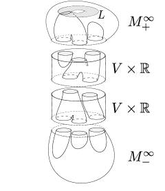
Figure 6: A stable curve of height 2 + 2. A possible limit of a sequence of $J^{n}$-holomorphic discs.

For a precise definition of stable curve of height $k$ (holomorphic building of height $\underset{1}{\overset{k-2}{\vee}}$) we refer the reader to section 1.6 of [7] (section 9 of [3]) - see also section 4.1 of [16]. For the notion of convergence, we refer the reader to the end of section 9.1 of [3].

Figure 6 illustrates a typical stable curve of height 4. It basically consists of a set of $J^{\infty}$-holomorphic maps from punctured, possibly disconnected, Riemann surfaces $\Sigma_{1},\dots\Sigma_{k}$ to $B_{1}=M_{-}^{\infty},B_{2}=V\times\mathbb{R},\dots,B_{k-1}=V\times\mathbb{R},B_{k}=M_{+}^{\infty}$, that are asymptotic to Reeb orbits at the punctures. We label a puncture positive/negative if it is asymptotic to a positive/negative end of $B_{i}$. A negative puncture of $\Sigma_{i}$ is associated with a positive puncture of $\Sigma_{i+1}$, both asymptotic to the same Reeb orbit under the respective maps. Also, $J^{\infty}$ is defined in $B_{i}=V\times\mathbb{R}$, $1<i<k$, using translation invariance.

4 Proof of Theorem 1.1

Before starting the setup for the proof of Theorem 1.1, we want to state some important preliminary results.

4.1 Preliminary results

Recall that we want to distinguish the tori by studying Maslov index 2 discs they bound and applying Theorem 6.4 of [15], which follows from the work of Gromov [11] - see also Proposition 4.1 A of [8].

Lemma 4.1.

(Theorem 6.4 of [15])

Let $L_{0}$ and $L_{1}$ be symplectomorphic monotone Lagrangian submanifolds of a symplectic manifold $(X,\omega)$, with an almost complex structure $J$ so that $(L_{0},J)$ and $(L_{1},J)$ are regular. Denote by $\varphi:X\rightarrow X$ be a symplectomorphism with $\varphi(L_{0})=L_{1}$. Then the algebraic counts of Maslov index 2 $J$-holomorphic discs in the classes $\beta\in\pi_{2}(X,L_{0})$ and $\varphi_{*}\beta\in\pi_{2}(X,L_{1})$ are the same.

In particular, we can arrange for new invariants of a monotone Lagrangian submanifold.

Definition 4.2.

Let $L$ be a Lagrangian submanifold of a symplectic manifold $X$, endowed with an almost complex structure $J$. The boundary Maslov-2 convex hull of a $L$ is the convex hull in $\pi_{1}(L)$ generated by the set {$\partial\beta\in\pi_{1}(L)\ |\ \beta\in\pi_{2}(X,L)$, such that the algebraic count of Maslov index 2 $J$-holomorphic discs in the class $\beta$ is non-zero }.

As an immediate consequence of Lemma 4.1 and the commutative diagram

we have the following Corollaries.

Corollary 4.3.

Using the same notation as in Lemma 4.1, for $L_{0}$ and $L_{1}$ symplectomorphic monotone Lagrangian submanifolds of $X$, the map $\varphi_{*}:\pi_{1}(L_{0})\rightarrow\pi_{1}(L_{1})$, sends the boundary Maslov-2 convex hull of $L_{0}$ to the boundary Maslov-2 convex hull of $L_{1}$.

Remark 4.4.

In particular, if we are given a basis for $\pi_{1}(L_{0})$ and a basis for $\pi_{1}(L_{1})$, we can see both $\pi_{1}(L_{i})$’s as the standard lattice $\mathbb{Z}^{m}\subset\mathbb{R}^{m}$, for some $m$. Call $\mho_{L_{i}}$ the image of the boundary Maslov-2 convex hull of $L_{i}$, $i=0,1$. Then Corollary 4.3 says that $\mho_{L_{0}}=A\mho_{L_{1}}$ for some $A\in SL(m,\mathbb{Z})$.

Remark 4.5.

In the case of $L$ a Lagrangian in $X$ simply connected symplectic manifold, we can choose an isomorphism $\pi_{2}(X,L)\cong\pi_{2}(X)\oplus\pi_{1}(L)$ with classes $\alpha_{i}\in\pi_{2}(X,L)$, $i=1,\dots,m$ mapping to a basis for $\pi_{1}(L)$. We can then identify $\pi_{1}(L)$ with the standard lattice $\mathbb{Z}^{m}\subset\mathbb{R}^{m}$. By writing the superpotential of $L$ (see Definition 3.3 of [2] or Definition 2.1 of [15]) with respect to coordinates $z_{\alpha_{i}}$ corresponding to $\alpha_{i}$ (in the sense of Lemma 2.7 of [2] or equation (2-2) in [15]), we can identify the boundary Maslov-2 convex hull of $L$ with the Newton polytope of the superpotential of $L$.

We will also make use of a result given by Cho-Poddar in [6] that classifies Maslov index 2 of holomorphic discs lying on the smooth part of a toric orbifold:

Lemma 4.6 (Corollary 6.4 of [6]).

Let $X$ be a toric orbifold of complex dimension $n$, endowed with its standard complex structure, and with moment polytope whose facets are orthogonal to the primitive vectors $\{\textbf{v}_{1},\cdots,\textbf{v}_{m}\}$. Then, up to the $T^{n}$-action, the smooth Maslov index 2 holomorphic discs (not passing through an orbifold point) are in one-to-one correspondence with the vectors $\{\textbf{v}_{1},\cdots,\textbf{v}_{m}\}$.

4.2 The setup

Consider the standard toric fibration of the orbifold $\mathbb{CP}(a^{2},b^{2},c^{2})$, for $(a,b,c)$ a Markov triple, represented by the left picture of Figure 4. We proceed as in Corollary 2.5. Perform a rational blowdown - see Figure 2 - on a neighbourhood of each vertex bounded by lens spaces of the form $L(a^{2},al_{1}-1),L(b^{2},bl_{2}-1),L(c^{2},cl_{3}-1)$ - see Proposition 2.2. Also, assume that the neighbourhoods are the quotient of balls of some small radius in the standard coordinate chart centered in the respective vertex (of the form $\mathbb{C}(k^{2},kl-1)$ for $k=a,b,c$), as in the paragraph before the Corollary 3.2. That way, we obtain an almost toric fibration of $\mathbb{CP}^{2}$ containing $T(a^{2},b^{2},c^{2})$ as a monotone fiber, as depicted in the left base diagram of Figure 7.

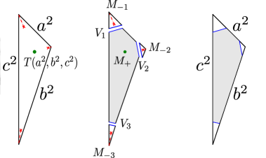
Figure 7: On the left, an almost toric fibration with $T(a^{2},b^{2},c^{2})$ as the central fiber. The middle diagram shows how the contact hypersurface $V=V_{1}\cup V_{2}\cup V_{3}$ separates $\mathbb{CP}^{2}$ in $M_{+}$ and $M_{-}=M_{-1}\cup M_{-2}\cup M_{-3}$. The right most diagram shows $M_{+}$ symplectically embedded into $\mathbb{CP}(a^{2},b^{2},c^{2})$.

Take $V=V_{1}\cup V_{2}\cup V_{3}$ the disconnected hypersurface in $\mathbb{CP}^{2}$ given by the union of the three lens spaces $V_{1}=L(a^{2},al_{1}-1),V_{2}=L(b^{2},bl_{2}-1),V_{3}=L(c^{2},cl_{3}-1)$, used for the symplectic rational blowdown. So $V$ divides $\mathbb{CP}^{2}$ in four connected components, which we name $M_{+}\cup M_{-1}\cup M_{-2}\cup M_{-3}$, as in the middle diagram of Figure 7. Consider the symplectic embedding of $M_{+}$ into $\mathbb{CP}(a^{2},b^{2},c^{2})$. We take the contact structure in $V$ and the almost complex structure $J$ on $M_{+}$ coming from the standard ones of $\mathbb{CP}(a^{2},b^{2},c^{2})$. They are adjusted in the sense given in section 3.2 (we need to take $X$ a multiple of the Liouville vector field) - see example 3.3. Since the space of compatible almost complex structures is contractible, we have no obstruction to extend $J$ defined on $M_{+}$ to $\mathbb{CP}^{2}$. Hence, we are in shape for applying neck-stretching for $M=\mathbb{CP}^{2}$, $V$ and $M_{+}$ as above, $M_{-}=M_{-1}\cup M_{-2}\cup M_{-3}$, and $J$, such that, restricted to $M_{+}$, is given by the pullback of the standard complex structure in $\mathbb{CP}(a^{2},b^{2},c^{2})$ via the embedding $M_{+}\hookrightarrow\mathbb{CP}(a^{2},b^{2},c^{2})$.

Lemma 4.7.

For $M$, $V$ and $J$ as above, we have that $(M_{+}^{\infty},\omega_{+}^{\infty},J_{+}^{\infty})$ is a Kähler manifold isomorphic to $(\mathbb{CP}(a^{2},b^{2},c^{2})\setminus\{p_{1},p_{2},p_{3}\},$ $\omega_{std},i)$, where $p_{1},p_{2},p_{3}$ are the pre-images of the vertices of the moment polytope under the standard moment map.

Proof.

Follows from Corollary 3.2. ∎

4.3 The proof

We proceed to the proof of

Theorem (1.1).

If $(a,b,c)$ and $(d,e,f)$ are two distinct Markov triples then the monotone Lagrangian tori $T(a^{2},b^{2},c^{2})$ and $T(d^{2},e^{2},f^{2})$ are not Hamiltonian isotopic.

Proof.

We recall that, for a monotone torus, Maslov index 2 discs have the same area. For convenience, we normalize the symplectic forms of $M=\mathbb{CP}^{2}$ and $\mathbb{CP}(a^{2},b^{2},c^{2})$, so that the symplectic area of Maslov index 2 discs is 1.

Figure 8: Picture of an almost toric diagram for $M^{n}$, which is $\mathbb{CP}^{2}$ after we inserted three necks of length $2n$ along $V_{1},V_{2},V_{3}$. The dot in the middle of the diagram represents $T(a^{2},b^{2},c^{2})$. The segments meeting at the dot are the images of pseudo-holomorphic discs in $M^{n}$ bounded by $T(a^{2},b^{2},c^{2})$.

Now we note that, by our embedding of $M_{+}$ (symplectic and holomorphic) into $\mathbb{CP}(a^{2},b^{2},c^{2})$, the image of $T(a^{2},b^{2},c^{2})$ is the standard monotone torus in $\mathbb{CP}(a^{2},b^{2},c^{2})$. Hence it bounds 3 one-parameter family of Maslov index 2 holomorphic discs, coming from the ones in $\mathbb{CP}(a^{2},b^{2},c^{2})$ that do not pass through an orbifold point (assuming we took a small enough neighbourhood for the rational blowdown) - see Figure 8 and Lemma 4.6. By Proposition 8.3 of [6], all discs of the above mentioned families are regular. We choose one holomorphic disc in each of the above one-parameter families. We write $\alpha,\beta,\gamma$ for the pullbacks of these three discs to $M_{+}\subset\mathbb{CP}^{2}$.

Insert necks of length $2n$ along $V_{1}$, $V_{2}$, $V_{3}$ as in described in section 3.1, obtaining $(M^{n},e^{-n}\omega^{n},J^{n})$.

Consider symplectomorphisms $\phi^{n}:M\longrightarrow M^{n}$, leaving $M_{+}\setminus\mathcal{N}$ invariant (recall that we identify $M_{+}\subset M$ with $M_{+}\subset M^{n}$), where $\mathcal{N}$ is a small neighbourhood of $V$ of the form $\mathcal{N}\cong V_{1}\times(-\epsilon,\epsilon)\cup V_{2}\times(-\epsilon,\epsilon)\cup V_{3}\times(-\epsilon,\epsilon)$. We also refer to $M_{-}\subset M^{n}$, but note that the symplectic form defined on $M_{-}\subset M^{n}$ differs by a factor of $e^{-2n}$ from the one defined on $M_{-}\subset M$ - see the definition of $M^{\tau}$ in section 3.1. Assume also that $\mathcal{N}$ is disjoint from $\alpha\cup\beta\cup\gamma$ (and the other discs that came from the embedding $M_{+}\hookrightarrow\mathbb{CP}(a^{2},b^{2},c^{2})$).

The following Lemma (for $n=0$) says that if a $J$-holomorphic disc is not in the classes $[\alpha]$, $[\beta]$ or $[\gamma]$, then its image must go through $V=V_{1}\cup V_{2}\cup V_{3}$.

Lemma 4.8.

Suppose that $u^{n}:(\mathbb{D},\partial\mathbb{D})\longrightarrow(M^{n},T(a^{2},b^{2},c^{2}))$ is a Maslov index 2 J-holomorphic disc whose image does not intersect $M_{-}\setminus\mathcal{N}\subset M^{n}$. Then it is a disc in one of the one-parameter families that contains either $\alpha$, $\beta$ or $\gamma$.

Proof.

Consider the contact hypersurface $V\times\{-\epsilon\}$ (which is the boundary of $M_{-}\setminus\mathcal{N}\subset M^{n}$) inside $(M^{n},e^{-n}\omega^{n},J^{n})$ and stretch the neck. We avoid developing all the notation for this particular neck-stretching, but let’s call the ‘$+$’ component of the neck stretching in the limit by $(M_{+}^{n+\infty},\omega_{+}^{n+\infty},J_{+}^{n+\infty})$. Since the image of $u^{n}$ does not intersect $M_{-}\setminus\mathcal{N}\subset M^{n}$, we can identify $u^{n}$ with the limit $u^{n+\infty}_{+}:(\mathbb{D},\partial\mathbb{D})\longrightarrow(M^{\infty}_{+},T(a^{2},b^{2},c^{2}))$, a $J^{n+\infty}_{+}$-holomorphic disc. As in Lemma 4.7, we are able to conclude that $(M_{+}^{n+\infty},\omega_{+}^{n+\infty},J_{+}^{n+\infty})\cong(M_{+}^{\infty},\omega_{+}^{\infty},J_{+}^{\infty})\cong(\mathbb{CP}(a^{2},b^{2},c^{2})\setminus\{p_{1},p_{2},p_{3}\}$. Therefore, we can identify $u^{n}$ with an holomorphic disc in $\mathbb{CP}(a^{2},b^{2},c^{2})$ lying in the smooth part. The result follows from Lemma 4.6.

∎

By Lemma 4.8 for $n=0$, the discs contained in the complement of $M_{-}\subset M$ are all regular. So, in order to obtain transversality we only need to perturb $J$ on $M_{-}$. Therefore, we can take a regular $J$, still having the property that, restricted to $M_{+}$, $J$ is given by the pullback of the standard complex structure in $\mathbb{CP}(a^{2},b^{2},c^{2})$, via the embedding $M_{+}\hookrightarrow\mathbb{CP}(a^{2},b^{2},c^{2})$.

Now consider a $J$-holomorphic disc $u$ of symplectic area 1. Set $[u]=[\text{Im}(u)]\in\pi_{2}(\mathbb{CP}^{2},T(a^{2},b^{2},c^{2}))$, and $[\partial u]\in\pi_{1}(T(a^{2},b^{2},c^{2}))$, the class of the boundary of $u$.

Take the isomorphism

$$\psi=\pi_{2}(\mathbb{CP}^{2},T(a^{2},b^{2},c^{2}))\overset{\cong}{\longrightarrow}\pi_{2}(\mathbb{CP}_{2})\oplus\pi_{1}(T(a^{2},b^{2},c^{2}))$$ (4.1)

that maps $\beta\to(0,\partial\beta)$ and $\gamma\to(0,\partial\gamma)$. Via this identification, we completely determine the class of a disc of symplectic area 1 by its projection to the second factor, i.e., by its boundary.

Lemma 4.9.

Assume that the algebraic count of $J$-holomorphic discs in $[u]$ is non-zero. Then, the class $[\partial u]$ lies in the convex hull generated by $[\partial\alpha]$, $[\partial\beta]$, $[\partial\gamma]$ in $\pi_{1}(T(a^{2},b^{2},c^{2}))\cong\mathbb{Z}^{2}$.

Proof.

We first observe that there is a $(\phi^{n})^{*}J^{n}$-holomorphic disc $\tilde{u}^{n}$ representing $[u]$: if $(\phi^{n})^{*}J^{n}$ is regular then, since the algebraic count of discs is nonzero, this follows from Lemma 4.1; if it is not regular then there must be a disc or else the condition of regularity is vacuously true. Therefore, $u^{n}=\phi^{n}\circ\tilde{u}^{n}:(\mathbb{D},\partial\mathbb{D})\longrightarrow(M^{n},T(a^{2},b^{2},c^{2}))$ is $J^{n}$-holomorphic.

By Theorem 3.4, there exists a subsequence that converges to a stable curve of height $k$, for some $k\geq 1$. In particular, it gives a $J_{+}^{\infty}$-holomorphic map $u_{+}^{\infty}:\Sigma\longrightarrow M_{+}^{\infty}$, where $\Sigma$ is a (possibly disconnected) punctured Riemann surface with boundary that consists of a circle mapped by $u_{+}^{\infty}$ to the limit of $T(a^{2},b^{2},c^{2})$, which we call $L(a^{2},b^{2},c^{2})$. One component of $\Sigma$ is a punctured disc, while the others, if any exist, are punctured spheres, because they cannot have positive genus.

By Lemma 4.7, we have that $(M_{+}^{\infty},\omega_{+}^{\infty},$ $J_{+}^{\infty})$ is a Kähler manifold isomorphic to $(\mathbb{CP}(a^{2},b^{2},c^{2})\setminus\{p_{1},p_{2},p_{3}\},$ $\omega_{std},i)$, where $p_{1},p_{2},p_{3}$ are the pre-images of the vertices of the moment polytope under the standard moment map.

Hence, we can compactify $(M_{+}^{\infty},\omega_{+}^{\infty},J_{+}^{\infty})$ to $(\mathbb{CP}(a^{2},b^{2},c^{2}),\omega_{std},i)$. We also extend $u_{+}^{\infty}$ to the (possibly disconnected) Riemann surface $\bar{\Sigma}$ as an holomorphic map in the sense of Definition 2.1.3 of [5] - see also Definition A of [4]. Topologically, we can see this map defining a class on $\pi_{2}(\mathbb{CP}(a^{2},b^{2},c^{2}),L(a^{2},b^{2},c^{2}))$, which we call $[u_{+}^{\infty}]$, since all the components of $\bar{\Sigma}$ that are not the disc are spheres (topologically, we could think the domain of the compactification of $u_{+}^{\infty}$ consists of chains of spheres attached to one disc). Moreover, under the identification of $T(a^{2},b^{2},c^{2})\subset\mathbb{CP}^{2}$ with $L(a^{2},b^{2},c^{2})\subset\mathbb{CP}(a^{2},b^{2},c^{2})$, we have that $\partial[u_{+}^{\infty}]=\partial[u]$.

Remark 4.10.

Note that the discs $\alpha,\beta,\gamma$ and the symplectic form in $M_{+}\subset M^{n}$, for all $n=0,1,2,\dots,\infty$, remain invariant. We keep calling $\alpha,\beta,\gamma$ their own limit in $\mathbb{CP}(a^{2},b^{2},c^{2})$.

Call $D_{1}$, $D_{2}$, $D_{3}$ the inverse images of the (closed) edges of the moment polytope of $\mathbb{CP}(a^{2},b^{2},c^{2})$, which are (pseudo)-holomorphic curves in the sense of Definition A of [4] (essentially the same of Definition 2.1.3 of [5]). Also, by Definition A of [4], the image of $u_{+}^{\infty}$ is a (pseudo)-holomorphic curve. We will abuse notation and say that $u_{+}^{\infty}$ is a holomorphic curve in $\mathbb{CP}(a^{2},b^{2},c^{2})$.

In Definition B of [4], Chen gives a notion of algebraic intersection number (which is a rational number) for pseudo-holomorphic curves in an orbifold. We note that, up to relabeling, the intersection number of $\alpha,\beta,\gamma$ with $D_{1}$, $D_{2}$, $D_{3}$ is $(1,0,0),(0,1,0)$ and $(0,0,1)$, respectively. Since $\alpha$, $\beta$ and $\gamma$ generate $\pi_{2}(\mathbb{CP}(a^{2},b^{2},c^{2}),L(a^{2},b^{2},c^{2}))$, the classes that have positive intersection with $D_{1}$, $D_{2}$, $D_{3}$ lie in the cone generated by $\alpha$, $\beta$ and $\gamma$. Moreover, this cone projects via $\partial:\pi_{2}(\mathbb{CP}(a^{2},b^{2},c^{2}),L(a^{2},b^{2},c^{2}))\rightarrow\pi_{1}(L(a^{2},b^{2},c^{2}))$, to the convex hull generated by $\partial\alpha$, $\partial\beta$, $\partial\gamma$. To prove Lemma 4.9, it therefore suffices to prove that $u_{+}^{\infty}$ intersects $D_{1}$, $D_{2}$, $D_{3}$ positively.

There is an intersection formula given by Chen on Theorem 3.2 of [4]. In particular, this formula implies that the algebraic intersection number of two pseudo-holomorphic curves in an orbifold is positive. Since $D_{1}$, $D_{2}$, $D_{3}$ and $u_{+}^{\infty}$ are holomorphic, their algebraic intersection number is positive. This implies Lemma 4.9, recalling that $[\partial u_{+}^{\infty}]=[\partial u]$ under the identification $T(a^{2},b^{2},c^{2})\cong L(a^{2},b^{2},c^{2})$.

∎

Lemma 4.11.

The algebraic count of discs in the classes $[\alpha]$, $[\beta]$ and $[\gamma]$ in $\pi_{2}(M,T(a^{2},b^{2},c^{2}))$ is $\pm 1$.

Proof.

Suppose that the algebraic count of discs in the class $[\alpha]$ is not $\pm 1$. Because the family of $\alpha$ counts with $\pm 1$ in all $M^{n}$ and the discs on that family are regular with respect to $J^{n}$, by Lemma 4.8, there must be $J^{n}$-holomorphic discs $u^{n}$ in the class $[\alpha]\in\pi_{2}(M^{n},T(a^{2},b^{2},c^{2}))$ intersecting $M_{-}\subset M^{n}$, for all $n$ (either to make $J^{n}$ irregular or by Lemma 4.1). Taking a limit of a subsequence, and compactifying $M_{+}^{\infty}$ to $\mathbb{CP}(a^{2},b^{2},c^{2})$ as in the proof of Lemma 4.9, we end up with a disc in the class $[\alpha]\in\pi_{2}(\mathbb{CP}(a^{2},b^{2},c^{2}),L(a^{2},b^{2},c^{2}))$ intersecting positively two of the complex curves $D_{1}$, $D_{2}$, $D_{3}$ (inverse images of the closed edges of the moment polytope of $\mathbb{CP}(a^{2},b^{2},c^{2})$). Contradiction. Clearly, the same argument works for classes $[\beta]$ and $[\gamma]$.

∎

We have the following as an immediate corollary of Lemma 4.9 and Lemma 4.11:

Corollary 4.12.

The boundary Maslov 2 convex hull of $T(a^{2},b^{2},c^{2})$ (Definition 4.2) is generated by $[\partial\alpha]$, $[\partial\beta]$ and $[\partial\gamma]$.

We can see that the boundary Maslov 2 convex hull of $T(a^{2},b^{2},c^{2})$ can be identified with the polytope dual to the moment polytope of $\mathbb{CP}(a^{2},b^{2},c^{2})$. The reader can check that the affine lengths of the edges of the convex hull associated to $T(a^{2},b^{2},c^{2})$ are $a$, $b$ and $c$. Then the Theorem 1.1 follows from Corollary 4.3 (which says that the boundary Maslov 2 convex hull is an invariant among monotone Lagrangians submanifolds). More precisely, first we choose our favourite basis for $\pi_{1}(T(a^{2},b^{2},c^{2}))$ and $\pi_{1}(T(d^{2},e^{2},f^{2})$ and see their respective boundary Maslov 2 convex hull inside $\mathbb{Z}^{2}$. After checking that the affine lengths of the edges are, respectively, $\{a,b,c\}$ and $\{d,e,f\}$, we conclude that, if $\{a,b,c\}\neq\{d,e,f\}$, then $T(a^{2},b^{2},c^{2})$ and $T(d^{2},e^{2},f^{2})$ are not symplectomorphic. This follows from Remark 4.4, because their boundary Maslov 2 convex hull inside $\mathbb{Z}^{2}$ are not related via an $SL(2,\mathbb{Z})$ action (note that $SL(2,\mathbb{Z})$ preserves affine length).

∎

References

- [1] D. Auroux, Infinitely many monotone Lagrangian tori in , 2014, arxiv.org/pdf/1407.3725.
- [2] D. Auroux. Mirror symmetry and T-Duality on the complement of an anticanonical divisor, J. Gökova Geom. Topol. GGT 1 (2007), 51-91,
- [3] F. Bourgeois, Y. Eliashberg, H. Hofer, K. Wysocki, E. Zehnder Compactness results in symplectic field theory, GAFA 2000 (Tel Aviv, 1999). Geom. Funct. Anal. 2000, Special Volume, Part II, 560-673.
- [4] W. Chen Orbifold adjunction formula and symplectic cobordism between lens spaces, Geometry and Topology 8 (2004), 710-734.
- [5] W. Chen, Y. Ruan Orbifold Gromov-Witten theory, in Orbifolds in Mathematics and Physics, Adem, A. et al ed., Contemporary Mathematics 310, pp 25-85. Amer. Math. Soc., Providence, RI, 2002.
- [6] C. Cho; M. Poddar. Holomorphic orbi-discs and Lagrangian Floer cohomology of symplectic toric orbifolds, Journal of Differential Geometry 98 (2014), no. 1, 21–116. http://projecteuclid.org/euclid.jdg/1406137695.
- [7] Y. Eliashberg, A. Givental, H. Hofer, Introduction to symplectic field theory, GAFA 2000 (Tel Aviv, 1999). Geom. Funct. Anal. 2000, Special Volume, Part II, 560-673.
- [8] Y. Eliashberg, L. Polterovich. The problem of Lagrangian knots in four-manifolds, Geometric Topology (Athens, 1993), AMS/IP Stud. Adv. Math., Amer. Math. Soc., 1997, pp. 313-327
- [9] S. Galkin, A. Usnich, Mutations of potentials, Preprint IPMU 10-0100, 2010.
- [10] S. Galkin, G. Mikhalkin, in preparation.
- [11] M. Gromov, Pseudo-holomorphic curves in symplectic manifolds, Invent. Math. 82 (1985), 307 - 347.
- [12] N.C. Leung, M. Symington, Almost toric symplectic four-manifolds, Journal of symplectic geometry Volume 8, Number 2, 143-187, 2010.
- [13] J. Oakley, M. Usher, On Certain Lagrangian Submanifolds of and , 2013, arxiv.org/pdf/1311.5152.
- [14] M. Symington, Four dimensions from two in symplectic topology, in Proceedings of the 2001 Georgia International Topology Conference, Proceedings of Symposia in Pure Mathematics, Amer. Math. Soc., Providence, RI, 2003, 153-208.
- [15] R. Vianna, On Exotic Lagrangian Tori in , Geometry and Topology 18 (2014) 2419-2476.
- [16] W. Wu, On an exotic Lagrangian torus in , 2012, arxiv.org/pdf/1201.2446.