On the Intensity Distribution Functionof Blazed Reflective Diffraction Gratings

Abstract

We derive from first principles the expression for the angular/wavelength distribution of the intensity diffracted by a blazed reflective grating, according to a scalar theory of diffraction. We considered the most common case of a groove profile with rectangular apex. Our derivation correctly identifies the geometric parameters of a blazed reflective grating that determine its diffraction efficiency, and fixes an incorrect but commonly adopted expression in the literature. We compare the predictions of this scalar theory with those resulting from a rigorous vector treatment of diffraction from one-dimensional blazed reflective gratings.

I Introduction

Diffraction gratings are widely used tools for astronomical applications, in both ground-based and space-borne telescope facilities. A proper implementation of gratings for spectroscopic observations requires a full understanding of their properties. However, apart from a few results following directly from the grating equation (spectral dispersion, free spectral range, blaze wavelength), the derivation of other important characteristics of gratings is less straightforward. This is certainly the case for the determination of the angular/wavelength distribution of the diffracted intensity, which is needed for the estimation of the grating efficiency under specific illumination conditions, and for given diffraction orders and directions. A reliable estimate of the grating efficiency is critical in the design of spectroscopic tools to be employed for observations that are particularly demanding on the photon flux reaching the detector. A typical example is that of high-sensitivity spectro-polarimetry, which is a fundamental diagnostic tool for the inference of magnetic fields in astrophysical plasmas.

A correct determination of the grating intensity distribution must take into account the polarization properties of gratings, and can only be attained within a full (vector) electro-magnetic theory of diffraction. However, the simpler scalar theory is often very useful, being capable of providing a good approximation to the average (i.e., unpolarized) efficiency, which can be adopted for reliable flux-budget estimations in spectrographic instruments. This is particularly true for small blaze angles, and for small ratios of the wavelength to the grating period LP97 . Echelle gratings with steeper blaze angles (e.g., of the R2 type, which is commonly adopted in high spectral resolution instrument setups for the remote sensing of astrophysical plasmas), working in relatively low orders, typically display strong polarization features and anomalies. However, special reflective coating techniques such as “shadow casting” Ke66 have been demonstrated to effectively reduce these anomalies to such a level that the scalar theory of diffraction becomes again useful also for the modeling of the efficiency of this type of gratings.

In the case of transmission gratings, the expression for the intensity distribution of the diffracted radiation is well-known Gr05 ; Sa06 ; Se10 , and it depends in a fundamental way on the grating period, $d$, and the width of the transmitting aperture, $b$. Unfortunately, the commonly used extension of that formula to blazed reflective gratings appears to be marred by a confused identification of the width $b$ Gr05 . This misuse of the intensity distribution function typically results in grossly overestimated or underestimated efficiencies for echelle gratings, ultimately affecting the reliability of the design of spectrographic instruments. Sc00 provides the correct identification of the $b$ parameter for blazed reflective gratings under different illumination conditions, although without formal derivation.

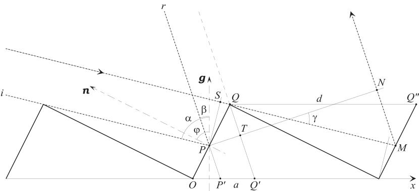
Figure 1: Geometric construction for the derivation of the grating efficiency formula. The grating shown in the figure has ruling step $d$ and blaze angle $\varphi$, with the two facets forming a right angle (in $Q$). $\alpha$ is the angle of incidence of the incoming light ($i$) measured from the normal $\bm{g}$ of the grating, while $\beta$ gives the direction of the diffracted light ($r$). $\bm{n}$ is the normal to the illuminated facet, so that $\varphi=\widehat{\bm{gn}}$.

In Section II, we derive from first principles the scalar intensity distribution function of a blazed reflective grating, for the most common case of a groove profile with rectangular apex. Comparing our result with the commonly adopted expression for this intensity distribution, we attain a clear identification of the geometric parameters involved. This derivation of the intensity distribution function for a blazed reflective grating is validated by the results of numerical modeling based on a vector theory of diffraction from one-dimensional diffraction gratings, which are presented in Section III, as well as from laboratory measurements (H. Lin, private communication).

II Theory

Figure 1 shows the geometric construction for a reflective diffraction grating with a blaze angle $\varphi$ and ruling period $d$. For simplicity, we assume the most common case of a grating profile with rectangular apex. Conventionally, we indicate with $\alpha$ the incidence angle of the incoming radiation ($i$) with respect to the grating normal $\bm{g}$, and with $\beta$ the corresponding angle for the diffracted radiation ($r$). In the following derivation we assume the condition $\alpha\geq\varphi$, which ensures that the secondary facet is never illuminated (and therefore does not contribute to the diffracted energy). The case $\alpha<\varphi$ will be discussed briefly at the end, in the context of shadowing.

Following Gr05 , the distribution of the diffracted intensity by a grating, according to the scalar theory of diffraction, can be obtained from the Fourier transform of the grating transmission (or aperture) function, $G(x)$, where $x$ is the coordinate along the grating plane (see Fig. 1). This transmission function is different from zero only in correspondence of the openings of the grating, i.e., the regions of the $x$-axis from where the diffracted radiation appears to emanate. These openings are the analog of the transmitting apertures in a transmission grating. For a blazed reflective grating, such as the one pictured in Fig. 1, we see that these openings correspond to the segment $P^{\prime}Q^{\prime}$ and periodic replicas of it along the grating length. The width and location of these segments are evidently functions of the angles $\alpha$ and $\beta$. In particular, the width is given by

$$a\equiv P^{\prime}Q^{\prime}=PQ\,\frac{\cos(\beta-\varphi)}{\cos\beta}\;,$$ (1)

whereas the position of the median points of the openings is located at $\bar{x}=[x(P^{\prime})+x(Q^{\prime})]/2$ and periodic replicas of it along the grating length, where

$$\bar{x}=x(P^{\prime})+\frac{a}{2} = d\sin\varphi\tan(\alpha-\varphi)(\cos\varphi+\sin\varphi\tan\beta)+\frac{d}{2}\,\frac{\cos\alpha}{\cos\beta}\,\frac{\cos(\beta-\varphi)}{\cos(\alpha-\varphi)}$$ (2)

$$= \frac{d}{2}\,\frac{\cos(\alpha-2\varphi)}{\cos\beta}\,\frac{\cos(\beta-\varphi)}{\cos(\alpha-\varphi)}\;.$$

In order to properly calculate the Fourier transform of the transmission function $G(x)$, we need to determine the phase dependence on $x$ of the diffracted wave across the width $P^{\prime}Q^{\prime}$. In order to do so, we must calculate the path difference between the incident and the diffracted wave after the plane $PS$, at which the incident (plane) wave is in phase. The segment $PQ$ illuminated by the incident light is given by

$$PQ = d\cos\varphi-d\sin\varphi\tan(\alpha-\varphi)$$ (3)

$$= d\,\frac{\cos\alpha}{\cos(\alpha-\varphi)}\;.$$

Therefore, from Fig. 1, the path differences for the diffracted beam are

$$SQ = PQ\sin(\alpha-\varphi)\;,$$ (4a)

$$TQ = PQ\sin(\varphi-\beta)\;.$$ (4b)

The overall phase difference between the points $T$ and $P$ in the diffracted wave for the wavelength $\lambda$ is thus

$$\theta(\varphi) = \frac{2\pi}{\lambda}\,(SQ-TQ)$$ (5)

$$= \frac{2\pi}{\lambda}\,PQ\,[\sin(\alpha-\varphi)+\sin(\beta-\varphi)]\;,$$

We note that for

$$\alpha-\varphi=\varphi-\beta\;,\quad\Longrightarrow\quad\alpha+\beta=2\varphi\;,$$ (6)

the phase $\theta(\varphi)$ vanishes identically. This is the ordinary condition of reflection on the grating facets (blaze condition).

For values of $x$ intermediate between $P^{\prime}$ and $Q^{\prime}$, the phase difference between the diffracted ray through $x$ and the one through $\bar{x}$ scales with the factor

$$\rho_{x}\equiv\frac{x-\bar{x}}{a}\;,\qquad x(P^{\prime})\leq x\leq x(Q^{\prime})\;,$$ (7)

which therefore must be introduced into Eq. (5), as a multiplicative scaling factor of $PQ$, in order to calculate the dephasing of the diffracted beam introduced by the blaze.

The derivation given above allows the computation of the phase dependence of an arbitrary diffracted ray through the segment $P^{\prime}Q^{\prime}$ for the groove that was conventionally set as the origin. Each successive groove introduces an offset of the phase retardance that is constant throughout the grating (i.e., independent of $x$), and which is determined by the additional travel of the plane wave over the path $SQ+QM+MN$. The segment $SQ$ has already been determined, whereas

$$QM=d\,\frac{\sin\varphi}{\cos(\alpha-\varphi)}\;.$$ (8)

Since $\gamma=90^{\circ}-(\alpha-\beta)$, we also have

$$TQ+MN=QM\cos(\alpha-\beta)\;,$$ (9)

where $TQ$ has also been determined earlier. The phase retardance introduced by each groove is therefore

$$\Theta = \frac{2\pi}{\lambda}\,(SQ+QM+MN)$$ (10)

$$= \frac{2\pi}{\lambda}\,[SQ-TQ+QM+(TQ+MN)]$$

$$= \frac{2\pi}{\lambda}\Bigl{\{}PQ\,[\sin(\alpha-\varphi)+\sin(\beta-\varphi)]+QM\,[1+\cos(\alpha-\beta)]\Bigr{\}}\;,$$

with $PQ$ and $QM$ given by Eqs. (3) and (8), respectively. With these substitutions, after some tedious algebra, we find simply

$$\Theta=\frac{2\pi}{\lambda}\,d\,(\sin\alpha+\sin\beta)\;.$$ (11)

The last expression can be cast into the usual form of the grating equation (e.g., Gr05 ), when we observe that the different orders $n$ of diffraction by the grating must correspond to phase conditions of constructive interference, i.e., $\Theta=2\pi n$, with $n$ an integer.

We now consider the explicit expression of the transmission function, $G(x)$, for a blazed grating. This is given by (cf. Gr05 , Eq. (3.3))

$$G(x)=a(x)\ast{\rm III}_{d}(x-\bar{x})\,U_{L}(x)\;,$$ (12)

where $a(x)$ is the “window” function associated with the segment $P^{\prime}Q^{\prime}$ of width $a$, ${\rm III}_{d}(x)=\sum_{n}\delta(x-nd)$ is the sampling function (Dirac’s comb) of the grating, and $U_{L}(x)$ is the box function of unit height that limits the total length, $L$, of the grating. For a blazed grating, $a(x)$ is not purely real, since it carries the additional dephasing due to the blaze with respect to the case of a flat grating. For the interval $x-\bar{x}$ this dephasing is evidently given by (see Eqs. (2) and (6))

$$\Delta\theta(x)\equiv\biggl{[}\frac{\theta(\varphi)}{a}-\frac{\Theta}{d}\biggr{]}(x-\bar{x})\;.$$ (13)

If $U_{a}(x)$ is the unit box of width $a$, then

$$a(x)=U_{a}(x)\,\hbox{e}^{{\rm i}\,\Delta\theta(x)}\;.$$ (14)

The Fourier transform of $G(x)$ is given by

$$\tilde{G} \equiv \mathscr{F}\bigl{\{}G(x)\bigr{\}}$$ (15)

$$= \mathscr{F}\bigl{\{}a(x)\bigr{\}}\Bigl{[}\mathscr{F}\bigl{\{}{\rm III}_{d}(x-\bar{x})\bigr{\}}\ast\mathscr{F}\bigl{\{}U_{L}(x)\bigr{\}}\Bigr{]}\;,\kern 14.22636pt$$

and must be evaluated at $\sigma=(\sin\alpha+\sin\beta)/\lambda\equiv\Theta/(2\pi d)$. Equation (13) can then be rewritten,

$$\Delta\theta(x)=\biggl{[}\frac{\theta(\varphi)}{a}-2\pi\sigma\biggr{]}(x-\bar{x})\;.$$ (16)

Using fundamental properties of the Fourier transform, for the various contributions to Eq. (15), we find:

$$\kern-28.45274pt\mathscr{F}\bigl{\{}a(x)\bigr{\}}(\sigma) = \hbox{e}^{{\rm i}\,\Delta\theta(0)}\,\mathscr{F}\biggl{\{}U_{a}(x)\exp\biggl{(}{\rm i}\,\biggl{[}\frac{\theta(\varphi)}{a}-2\pi\sigma\biggr{]}x\biggr{)}\biggr{\}}(\sigma)$$ (17a)

$$= \hbox{e}^{{\rm i}\,\Delta\theta(0)}\,\mathscr{F}\bigl{\{}U_{a}(x)\bigr{\}}\biggl{(}\frac{\theta(\varphi)}{2\pi a}\biggr{)}$$

$$= \hbox{e}^{{\rm i}\,\Delta\theta(0)}\,{\rm sinc}\biggl{(}\frac{\theta(\varphi)}{2}\biggr{)}\;;$$

$$\mathscr{F}\bigl{\{}{\rm III}_{d}(x-\bar{x})\bigr{\}}(\sigma) = \hbox{e}^{{\rm i}\,2\pi\sigma\bar{x}}\,\mathscr{F}\bigl{\{}{\rm III}_{d}(x)\bigr{\}}(\sigma)$$ (17b)

$$= \hbox{e}^{{\rm i}\,2\pi\sigma\bar{x}}\,{\rm III}_{1/d}(\sigma)\;;$$

$$\mathscr{F}\bigl{\{}U_{L}(x)\bigr{\}}(\sigma)={\rm sinc}(\pi L\sigma)\;.$$ (17c)

Ultimately, we are only interested in the intensity distribution function of the diffracted field, which is proportional to $|\tilde{G}|^{2}$, so the phase factors in Eqs. (17a) and (17b) can simply be dropped. We note that Eq. (17b) determines the free spectral range of the grating as a dispersing element, whereas Eq. (17c) determines its finesse (or resolution). The “envelope” of the diffracted light distribution is instead exclusively determined by Eq. (17a) (cf. Gr05 , Eqs. (3.4) and (3.8)), and this is the quantity we are interested in for the present study.

If we recall Eqs. (3) and (5), we find from Eq. (17a)

$$I(\beta) = {\rm sinc}^{2}\biggl{(}\frac{\pi d}{\lambda}\,\frac{\cos\alpha}{\cos(\alpha-\varphi)}\,[\sin(\alpha-\varphi)+\sin(\beta-\varphi)]\biggr{)}$$

$$= {\rm sinc}^{2}\biggl{(}n\pi\,\frac{\cos\alpha}{\cos(\alpha-\varphi)}\,\frac{\sin(\alpha-\varphi)+\sin(\beta-\varphi)}{\sin\alpha+\sin\beta}\biggr{)}$$

$$= {\rm sinc}^{2}\biggl{(}n\pi\,\frac{\cos\alpha}{\cos(\alpha-\varphi)}\biggl{[}\cos\varphi-\sin\varphi\cot\frac{\alpha+\beta}{2}\biggr{]}\biggr{)}\;,$$

where in the second equivalence we used the grating equation (cf. Eq. (11), and the discussion following that equation). If we recall the discussion following Eq. (5), Eq. (II) shows that, according to the scalar theory of gratings, the peak of the efficiency is reached at the blaze condition, $\alpha+\beta=2\varphi$. For a given grating configuration and diffraction order $n$, the efficiency peak then occurs at the so-called blaze wavelength

$$\lambda_{\rm b}\equiv\frac{d}{n}\,[\sin\alpha+\sin(2\varphi-\alpha)]\;.$$ (19)

We also note that, for $\lambda=\lambda_{\rm b}$, the Littrow condition, $\alpha=\beta$, also corresponds to the configuration of normal incidence on the grating facets, $\alpha=\varphi$, in which case

$$\lambda_{n}\equiv\lambda_{\rm b}^{\rm Litt}=\frac{2d}{n}\,\sin\varphi\;.$$ (20)

Comparison of Eq. (II) with Eq. (3.8) of Gr05 , shows that it must be, for $\alpha\geq\varphi$,

$$\frac{b}{d}=\frac{\cos\alpha}{\cos(\alpha-\varphi)}\;,$$ (21)

where $b$ is the effective width of the openings that must be adopted according to Gr05 in order to reproduce the correct envelope of the diffracted energy $I(\beta)$. From this we conclude that $b=PQ$, according to our derivation, i.e., the effective width of the openings in a blazed reflective grating corresponds to the width of the illuminated portion of the grating’s facet (see Eq. (3)). Equation (21) is in agreement with Eq. (13.4.10) of Sc00 .

In the condition of normal incidence on the grating facets, $\alpha=\varphi$, we have simply $b/d=\cos\varphi$. Gr05 reports instead $b/d=\cos^{2}\varphi$, suggesting that the author identifies $b$ with the normal projection of the illuminated portion of the facet onto the grating length (i.e., with the quantity $a=P^{\prime}Q^{\prime}$ of Fig. 1). In the following, we will indicate this as “Gray’s ansatz.” Of course, the difference between these two conflicting identifications of the parameter $b$ may lie below the limit of experimental detection for small blaze angles. Instead, in the case of echelle gratings, the difference in the estimated grating efficiencies provided by the two alternate formulations can be significant. In the next Section, we present comparisons with results from a rigorous vector model of grating diffraction, which support the validity of Eq. (21).

Interestingly, the same problem has also been treated by Br59 through a geometric argument similar to the one presented here. The author arrives at an expression for the ratio $b/d$ that is formally identical to Eq. (21), but where $\beta$ appears instead of $\alpha$. While this would still lead to the correct estimation of the $b/d$ ratio at the Littrow condition, in the general case it determines an unphysical behavior of the diffracted efficiency towards the wavelength corresponding to the “passing off” of a diffraction order, which ultimately violates energy conservation. In fact, it can be demonstrated that, for $\beta\to\pi/2$, Eq. (II) tends identically to unity, if $\alpha$ and $\beta$ are exchanged in that expression.

From the geometric construct of Fig. 1 we can also determine the grating magnification (also known as anamorphic magnification), which is defined as $r=PS/PN$. From the above derivation, we have $PS=PQ\cos(\alpha-\varphi)$, and $PN=PT+TN=PQ\cos(\varphi-\beta)+QM\sin(\alpha-\beta)$. After some simple algebra, we find the usual result

$$r=\frac{\cos\alpha}{\cos\beta}\;.$$ (22)

Figure 2: Efficiency curves for the orders 1 (thin curves) and 2 (thick curves) for an Al grating with 600 lines/mm and $\varphi=20^{\circ}$, used in the configuration of normal incidence on the grating facets, $\alpha=\varphi$. The theoretical TE ($p$) and TM ($s$) polarizations are shown, as well as the unpolarized case (corresponding to the average of the two polarizations; dash-dotted curves).

Figure 3: Same as Fig. 2, but using the scalar theory derived in this paper (continuous curves). An overall grating loss of 16.5% was introduced via a scaling factor, in order to match the efficiency peaks of the continuous curves to those of the unpolarized efficiency curves of Fig. 2 (dash-dotted curves in this plot). The dotted curves correspond to the grating efficiency determined by Gray’s ansatz for the expression of the ratio $b/d$ (see Eq. (21)). We note how the differences introduced by Gray’s ansatz are very small in this case, because of the small blaze angle.

Finally, the grating model given in Fig. 1 can also be used to determine the efficiency loss due to shadowing, which sets in when the illumination of the grating is such that $\alpha<\beta$. We first consider the case $\alpha<\varphi$, and apply the principle of reversibility in order to exchange the role of $\alpha$ and $\beta$ in Fig. 1. We then can conclude that only a fraction $P^{\prime}Q^{\prime}/d\equiv a/d$ of the incoming light is diffracted into the outgoing direction. From Eqs. (1) and (3), and taking into account the reversed roles of $\alpha$ and $\beta$, the reduction factor of the grating efficiency due to shadowing is therefore

$$s\equiv a/d = \frac{\cos\beta}{\cos\alpha}\,\frac{\cos(\alpha-\varphi)}{\cos(\beta-\varphi)}$$ (23)

$$= \frac{1}{r}\,\frac{\cos(\alpha-\varphi)}{\cos(\beta-\varphi)}\;.$$

where in the last line we used the definition of the grating magnification, Eq. (22). It is easy to demonstrate that Eq. (23) applies also to the case $\alpha\geq\varphi$. To see this, we must picture the geometric construct of Fig. 1 for the case $\beta>\alpha$, and observe that the unblocked portion of the diffracted beam appears to originate from a sub-region of the grating facet of width $P^{\prime\prime}Q$, such that (cf. Eq. (3))

$$P^{\prime\prime}Q=d\,\frac{\cos\beta}{\cos(\beta-\varphi)}<PQ=d\,\frac{\cos\alpha}{\cos(\alpha-\varphi)}\;.$$ (24)

In this case, the reduction factor of the grating efficiency due to shadowing is $s\equiv P^{\prime\prime}Q/PQ<1$, and the last equation shows that the expression of $s$ coincides with the RHS of Eq. (23) also for $\alpha\geq\varphi$.

Equation (23) shows that shadowing reduces the peak efficiency of a grating order by a factor $1/r=\cos\beta/\cos(2\varphi-\beta)$, because of the blaze condition $\alpha-\varphi=\varphi-\beta$. This result is in agreement with the treatment of shadowing given in Gr05 , as seen from Eq. (3.11) in that reference. However, that expression strictly holds only at the blaze condition, unlike Eq. (23) in this paper, which is instead general.

In conclusion, the expression of the grating efficiency, Eq. (II), must in general be multiplied by a scaling factor $k=\min(s,1)$, with $s$ given by Eq. (23). This reduction factor sets in under the shadowing condition $\alpha<\beta$, and applies identically in the two cases $\alpha\geq\varphi$ and $\alpha<\varphi$.

We then can rewrite the expression of the grating efficiency for the wavelength $\lambda$ or the diffraction order $n$ as

$$I(\beta) = k\;{\rm sinc}^{2}\biggl{(}\frac{\pi d}{\lambda}\,\rho\,[\sin(\alpha-\varphi)+\sin(\beta-\varphi)]\biggr{)}$$ (25)

$$= k\;{\rm sinc}^{2}\biggl{(}n\pi\,\rho\biggl{[}\cos\varphi-\sin\varphi\cot\frac{\alpha+\beta}{2}\biggr{]}\biggr{)}\;,\kern 14.22636pt$$

where $\rho\equiv b/d$ is given by Eq. (21) for $\alpha\geq\varphi$, while it remains at the maximum possible value $\cos\varphi$ for $\alpha<\varphi$.

Figure 4: Same as Fig. 2, but for the order 16 of an Ag grating with 200 lines/mm and $\varphi=60^{\circ}$, and under the illumination condition $\alpha=\varphi$.

Figure 5: Same as Fig. 4, but using the scalar theory as for the plots of Fig. 3 (continuous curve). An overall grating loss of 20% due to the reflective layer was considered for this calculation. In this case, the scalar theory is able to reproduce the unpolarized efficiency of the grating (dash-dotted curve), at least around the peak, if Eq. (21) is adopted for $b/d$. In contrast, the scalar theory is unable to reproduce both efficiency and position of the peak, as well as the FWHM of the efficiency profile, if Gray’s ansatz is used instead (dotted curve).

III Discussion and Conclusions

In this section we will consider some examples of grating efficiency calculations, in order to test the ability of the scalar theory of gratings presented above to reproduce results predicted by a rigorous (vector) treatment of light diffraction by one-dimensional gratings.

The formulation presented above reproduces rather well the average efficiency of blazed reflective gratings as derived from a full treatement of the electro-magnetic theory of diffraction, at the condition that energy conservation across the various orders and efficiency losses due to shadowing are taken into account, and that polarization effects introduced by the grating are not predominant. A good reproduction of the peak efficiency may need an additional scaling factor to account for the wavelength dependence of the reflectivity of the coating. Since this reflectivity does not enter explicitly the scalar theory of gratings, it must be introduced ad hoc as a normalization parameter.

Figure 2 shows the efficiency curves for the TE (or $p$) and TM (or $s$) polarizations of the diffracted field in the orders $n=1,2$ of an Al grating with 600 lines/mm and $\varphi=20^{\circ}$, used in the configuration of normal incidence on the grating facets (i.e., $\alpha=\varphi$). We recall that such configuration corresponds to a Littrow mount ($\alpha=\beta$) when $\lambda=\lambda_{n}$ (see Eq. (20)). The plots of Fig. 2 were calculated with a code based on the C-method for grating analysis as described in Li99 . For comparison, the continuous curves in Fig. 3 represent the scalar efficiencies calculated through Eq. (25), taking into account energy conservation, the energy loss due to shadowing as described by Eq. (23), and adding an overall grating loss of 16.5%. We note that in this case the scalar theory is able to reproduce adequately the position of the efficiency peak, as well as the full width at half maximum (FWHM) and overall trend of the unpolarized efficiency profile. The dotted curves in Fig. 3 show the predicted efficiency using Gray’s ansatz for the $b/d$ ratio (see discussion after Eq. (21)). For this grating – which is analogous to the one considered by Gr05 in his Figs. 3.11 and 3.12 – the differences between the two alternate definitions of $b/d$ are very small, as expected because of the small blaze angle of the grating (see note 2).

Figures 4 and 5 provide another test of the performance of the scalar theory of gratings. These new calculations are for a Ag grating with 200 lines/mm and a blaze angle $\varphi=60^{\circ}$. Also in this case, the grating is used in a configuration of normal incidence on the grating facets, which corresponds to a Littrow mount at the blaze wavelength $\lambda_{n}\approx 541.3$ nm for the case $n=16$ shown in the figure.

Comparing Figs. 4 and 5 we see that for echelle gratings the agreement between the scalar and vector theories of diffraction is significantly worse than in the case illustrated by Figs. 2 and 3. Nonetheless, the scalar theory is still capable of reproducing the efficiency curve in a neighborhood of the peak, as well as the FWHM of the efficiency profile, which is an important quantity for a correct estimation of the bandwidth of the diffraction orders. In contrast, use of Gray’s ansatz for echelle gratings gives results that are completely at variance with those of the vector theory. In particular, because of the much larger (by $\sim 60$%) FWHM of the efficiency profile determined by Gray’s ansatz, the overlap between distinct orders at any given wavelength is also much larger than in reality, so it becomes impossible to reproduce the peak efficiency simply because of energy conservation – i.e., the diffracted energy at any given wavelength gets distributed into too many orders. The position of the efficiency peak also misses to reproduce the results of the vector theory in this case, remaining practically located at $\lambda_{n}$.

- (1) E. G. Loewen and E. Popov, Diffraction Gratings and Applications, Dekker, New York (1997)
- (2) J. D. Keller and R. J. Meltzer, “Reflective Diffraction Grating for Minimizing Anomalies,” U.S. Patent 3,237,508 (1966)
- (3) D. F. Gray, The Observation and Analysis of Stellar Atmospheres, 3rd ed., Cambridge University Press, Cambridge (2005)
- (4) O. Sandfuchs, R. Brunner, D. Pätz, S. Sinzinger, and J. Ruoff, “Rigorous Analysis of Shadowing Effects in Blazed Transmission Gratings,” Opt. Lett. 31, 3638 (2006)
- (5) M. Seesselberg and B. H. Kleemann, “DOEs for Color Correction in Broad Band Optical Systems: Validity and Limits of Efficiency Approximations,” Proc. SPIE 7652, IODC (2010)
- (6) D. J. Schroeder, Astronomical Optics, 2nd ed., Academic Press, San Diego (2000)
- (7) G. Bruhat, Optique, Masson, Paris (1959)
- (8) L. Li, J. Chandezon, G. Granet, J.-P. Plumey, “Rigorous and efficient grating-analysis method made easy for optical engineers,” Appl. Opt. 38, 304-313 (1999)