The Filippov characteristic flow for the aggregation equation with mildly singular potentials

Abstract

Existence and uniqueness of global in time measure solution for the multidimensional aggregation equation is analyzed. Such a system can be written as a continuity equation with a velocity field computed through a self-consistent interaction potential. In Carrillo et al. (Duke Math J (2011)) [16], a well-posedness theory based on the geometric approach of gradient flows in measure metric spaces has been developed for mildly singular potentials at the origin under the basic assumption of being $\lambda$-convex. We propose here an alternative method using classical tools from PDEs. We show the existence of a characteristic flow based on Filippov’s theory of discontinuous dynamical systems such that the weak measure solution is the pushforward measure with this flow. Uniqueness is obtained thanks to a contraction argument in transport distances using the $\lambda$-convexity of the potential. Moreover, we show the equivalence of this solution with the gradient flow solution. Finally, we show the convergence of a numerical scheme for general measure solutions in this framework allowing for the simulation of solutions for initial smooth densities after their first blow-up time in $L^{p}$-norms.

Keywords: aggregation equation, nonlocal conservation equations, measure-valued solutions, gradient flow, Filippov’s flow, finite volume schemes.

2010 AMS subject classifications: 35B40, 35D30, 35L60, 35Q92, 49K20.

1 Introduction

This paper is devoted to the so-called aggregation equation in $d$ space dimension

$$\partial_{t}\rho=\mathop{\rm div}\nolimits\big{(}(\nabla_{x}W*\rho)\rho\big{)},\qquad t>0,\quad x\in\mathbb{R}^{d},$$ (1.1)

complemented with the initial condition $\rho(0,x)=\rho^{ini}$. Here, $W$ plays the role of an interaction potential whose gradient $\nabla_{x}W(x-y)$ measures the relative force exerted by an infinitesimal mass localized at a point $y$ onto an infinitesimal mass located at a point x.

This system appears in many applications in physics and population dynamics. In the framework of granular media, equation (1.1) is used to describe the large time dynamics of inhomogeneous kinetic models (see [4, 18, 44]). Model of crowd motion with a nonlinear dependancy of the term $\nabla_{x}W*\rho$ are also encountered in [20, 22]. In population dynamics, (1.1) provides a biologically meaningful description of aggregative phenomena. The description of the collective migration of cells by swarming leads to such non-local interaction PDEs (see e.g. [37, 38, 43]). Another example is the modelling of bacterial chemotaxis. In this framework, the quantity $S=W*\rho$ is the chemoattractant concentration which is a substance emitted by bacteria allowing them to interact with each others. The dynamics can be macroscopically modelled by the Patlak-Keller-Segel system [33, 39]. In the kinetic framework, the Othmer-Dunbar-Alt model is usually used, its hydrodynamic limit leads to the aggregation equation (1.1) [25, 26, 30]. In many of these examples, the potential $W$ is usually mildly singular, i.e. $W$ has a weak singularity at the origin. Due to this weak regularity, finite time blow-up of regular solutions has been observed for such systems and has gained the attention of several authors (see e.g. [34, 9, 6, 7, 16]). Finite time concentration is sometimes considered as a very simple mathematical way to mimick aggregation of individuals, as opposed to diffusion. Finally, attraction-repulsion potentials have been recently proposed as very simple models of pattern formation due to the rich structure of the set of stationary solutions, see [40, 13, 14, 3, 5] for instance.

Since finite time blow-up of regular solutions occurs, a natural framework to study the existence of global in time solutions is to work in the space of probability measures. However, several difficulties appear due to the weak regularity of the potential. In fact, the definition of the product of $\nabla W*\rho$ with $\rho$ is a priori not well defined. This fact has already been noticed in one dimension in [30, 31]. Using defect measures in a two-dimensional framework, existence of weak measure solutions for parabolic-elliptic coupled system has been obtained in [41, 24]. However, uniqueness is lacking. Measured valued solutions for the 2D Keller-Segel system have been considered in [36] as limit of solutions of a regularized problem.

For the aggregation equation (1.1), a well-posedness theory for measure valued solutions has been considered using the geometrical approach of gradient flows in [16]. This technique has been extended to the case with two species in [23]. The assumptions on the potential in order to get this well-posedness theory of measure valued solutions use certain convexity of the potential that allows for mild singularity of the potential at the origin.

In this paper, we assume that the interaction potential $W\,:\,\mathbb{R}^{d}\to\mathbb{R}$ satisfies the following properties:

• $W$ is Lipschitz continuous, $W(x)=W(-x)$ and $W(0)=0$.

• $W$ is $\lambda$-convex for some $\lambda\leq 0$, i.e. $W(x)-\frac{\lambda}{2}|x|^{2}$ is convex.

• $W\in C^{1}(\mathbb{R}^{d}\setminus\{0\})$.

Such a potential will be named as a pointy potential. A typical example is a fully attractive Morse type potential, $W(x)=1-e^{-|x|}$, which is $-1$-convex.

Let us emphasize that we only consider Lipschitz potentials which allows to bound the velocity field, whereas in [16], linearly growing at infinity potentials are allowed. In other words, we assume that there exists a nonnegative constant $w_{\infty}$ such that for all $x\neq 0$,

$$|\nabla W(x)|\leq w_{\infty}.$$ (1.2)

The main reason for this restriction is to be able to work with suitable characteristics for this velocity field as explained below.

Denoting $a=-\nabla W*\rho$ the macroscopic velocity, equation (1.1) can be considered as a conservative transport equation with velocity field $a$. Then a traditional definition for solutions is the one defined thanks to the characteristics corresponding to this macroscopic velocity. However, the velocity $a$ is not Lipschitz and therefore we cannot defined classical solutions to the characteristics equation. To overcome this difficulty, Filippov [27] has proposed a notion of solution which extend the classical one. Using this so-called Filippov flow, Poupaud & Rascle [42] have proposed a notion of solution to the conservative linear transport equation defined by $X_{\#}\rho^{ini}$ where $X$ is the Filippov flow corresponding to the macroscopic velocity. However a stability result of the flow was still lacking until recently [8], and thus there are no results with this technique for nonlinear equations of the form (1.1). We notice that in one dimension and for linear equations, these solutions are equivalent to the duality solutions defined in [11, 12], which have been successfully used in [30, 31] to tackle (1.1) in the one dimensional case.

On the other hand, although the geometric approach of gradient flows furnishes a well-posedness framework for well-posedness, this approach does not allow to define a characteristic flow corresponding to the macroscopic velocity $a=-\nabla W*\rho$. In this work, we focus on improving the understanding of these solutions by showing that under assumptions (A0)-(A2) on the potential, the solutions can be understood as their initial data pushed forward by suitable characteristic flows.

In order to achieve this goal, we first generalize the theory developed in [42] to the nonlinear aggregation equation (1.1). The first difficulty is, as it was in [16], to identify the right definition of the nonlinear term and the nonlinear product. This was solved in [16] by identifying the element of minimal norm by subdifferential calculus. We revisit this issue by clarifying that this is the right definition of the nonlinear term if we approximate a pointy potential by smooth symmetric potentials. Once the identification of the right velocity field has been done, we use the crucial stability results of Filippov’s flows in [8] to pass to the limit in the nonlinear terms. This leads to the construction of global measure solutions of the form $X_{\#}\rho^{ini}$, where $X$ is the Filippov flow associated to the velocity vector field $a$. This is the point where we need globally bounded velocity vector fields since Filippov’s theory [27] was only developed under these assumptions. In this way, we extend to the muti-dimensional case the results in [30] (for a particular choice of the potential $W$) and in [31].

Moreover, we are able to adapt arguments for uniqueness already used for the aggregation equation and for nonlinear continuity equations as in [35, 19, 7] to show the contraction property of the Wasserstein distance for our constructed solutions. This leads to a uniqueness result for our constructed solutions and to show the equivalence between the notion of gradient flow solutions and these Filippov’s flow characteristics solutions. Let us further comment that in the one dimensional case it has been noticed that there is a link between solutions to (1.1) and entropy solutions to scalar conservation law for an antiderivative of $\rho$ (see [9, 10, 30, 31]). This link has allowed to consider extensions of the model (1.1) with a nonlinear dependency of the term $\nabla W*\rho$.

Finally, let us mention that apart from particle methods to the aggregation equations, very few numerical schemes have been proposed to simulate solutions of the aggregation equation after blow-up. The so-called sticky particle method was shown to be convergent in [16] and used to obtain qualitative properties of the solutions such as the finite time total collapse. However, this method is not that practical to deal with finite time blow-up and the behavior of solutions after blow-up in dimensions larger than one. In one dimension, such numerical simulations thanks to a particle scheme have been obtained by part of the authors in [30]. Moreover, in the one dimensional case and with a nonlinear dependency of the term $\nabla W*\rho$, they propose in [32] a finite volume scheme allowing to simulate the behaviour after blow up and prove its convergence. Finally, extremely accurate numerical schemes have been developed to study the blow-up profile for smooth solutions, see [28, 29]. In fact, part of the authors recently proposed an energy decreasing finite volume method [15] for a large class of PDEs including in particular (1.1) but no convergence result was given. Here, we give a convergence result for a finite volume scheme and for general measures as initial data. This allows for numerical simulations of solutions in dimension greater than one allowing to observe the behaviour after blow-up occurs.

The outline of the paper is the following. Next section is devoted to the definition of our notion of weak measure solutions for the aggregation equation. After introducing some notations, we first recall the basic results as obtained by Poupaud & Rascle [42] on measure solutions for conservative linear transport equations. Then we define the notion of solutions defined by a flow and state the main result of this paper in Theorem 2.5. Finally, we recall the existence result of gradient flow solutions in [16] and state their equivalence with solutions defined by a flow. Section 3 is devoted to the proof of the existence and uniqueness result. The main ingredient of the proof of existence is a one-sided Lipschitz property of the macroscopic velocity and an atomization strategy by approximating with finite Dirac Deltas. A contraction argument in Wasserstein distance for these solutions allows to recover the uniqueness. In Section 4, we investigate the numerical approximation of such solutions. A finite volume scheme is proposed and its convergence is established for general measure valued solutions. An illustration thanks to numerical simulations is also provided showing the ability of the scheme to capture the finite time total collapse and the qualitative interaction between different aggregates after the first blow-up in $L^{p}$-norms. Finally, an Appendix is devoted to some technical Lemmas useful throughout the paper.

2 Weak measure solutions for the aggregation equation

All along the paper, we will make use of the following notations. We denote ${\cal M}_{loc}(\mathbb{R}^{d})$ the space of local Borel measures on $\mathbb{R}^{d}$. For $\rho\in{\cal M}_{loc}(\mathbb{R}^{d})$, we denote by $|\rho|(\mathbb{R}^{d})$ its total variation. We denote ${\cal M}_{b}(\mathbb{R}^{d})$ the space of measures in ${\cal M}_{loc}(\mathbb{R}^{d})$ with finite total variation. From now on, the space of measures ${\cal M}_{b}(\mathbb{R}^{d})$ is always endowed with the weak topology $\sigma({\cal M}_{b},C_{0})$. For $T>0$, we denote ${\cal S}_{\cal M}:=C([0,T];{\cal M}_{b}(\mathbb{R}^{d})-\sigma({\cal M}_{b},C_{0}))$. Finally, we define the space of probability measures with finite second order moment:

$${\cal P}_{2}(\mathbb{R}^{d})=\left\{\mu\mbox{ nonnegative Borel measure},\mu(\mathbb{R}^{d})=1,\int|x|^{2}\mu(dx)<\infty\right\}.$$

This space is endowed with the Wasserstein distance $d_{W}$ defined by (see e.g. [45, 46])

$$d_{W}(\mu,\nu)=\inf_{\gamma\in\Gamma(\mu,\nu)}\left\{\int|y-x|^{2}\,\gamma(dx,dy)\right\}^{1/2}$$ (2.1)

where $\Gamma(\mu,\nu)$ is the set of measures on $\mathbb{R}^{d}\times\mathbb{R}^{d}$ with marginals $\mu$ and $\nu$, i.e.

$$\Gamma(\mu,\nu)=\left\{\gamma\in{\cal P}_{2}(\mathbb{R}^{d}\times\mathbb{R}^{d});\ \forall\,\xi\in C_{0}(\mathbb{R}^{d}),\right. \int\xi(y_{0})\gamma(dy_{1},dy_{2})=\int\xi(y_{1})\mu(dy_{1}),$$

$$\left.\int\xi(y_{2})\gamma(dy_{1},dy_{2})=\int\xi(y_{2})\nu(dy_{2})\right\}.$$

From a minimization argument, we know that in the definition of $d_{W}$ the infimum is actually a minimum. A map that realizes the minimum in the definition (2.1) of $d_{W}$ is called an optimal plan, the set of which is denoted by $\Gamma_{0}(\mu,\nu)$. Then for all $\gamma_{0}\in\Gamma_{0}(\mu,\nu)$, we have

$$d_{W}^{2}(\mu,\nu)=\int|y-x|^{2}\,\gamma_{0}(dx,dy).$$

2.1 Weak measure solutions for conservative transport equation

We recall in this Section some useful results on weak measure solutions to the conservative transport equation

$$\partial_{t}u+\mathop{\rm div}\nolimits(bu)=0;\qquad u(t=0)=u^{0}.$$ (2.2)

We assume here that the vector field $b$ is given.

We start by the following definition of characteristics [27] :

Definition 2.1

Let us assume that $b=b(t,x)\in\mathbb{R}^{d}$ is a vector field defined on $[0,T]\times\mathbb{R}^{d}$ with $T>0$. A Filippov characteristic $X(t;s,x)$ stems from $x\in\mathbb{R}^{d}$ at time $s$ is a continuous function $X(\cdot;s,x)\in C([0,T],\mathbb{R}^{d})$ such that $\frac{\partial}{\partial t}X(t;s,x)$ exists a.e. $t\in[0,T]$ satisfying

$$\frac{\partial}{\partial t}X(t;s,x)\in\big{\{}{\mbox{C}onvess}(b)(t,\cdot)\big{\}}(X(t;s,x))\quad\mbox{a.e. }t\in[0,T];\qquad X(s;s,x)=x.$$

From now on, we will use the notation $X(t,x)=X(t;0,x)$.

In this definition $Convess(E)$ denotes the essential convex hull of a set $E$. We remind the reader the definition for the sake of completeness, see [27, 2] for more details. We denote by $Conv(E)$ the classical convex hull of $E$, i.e., the smallest closed convex set containing $E$. Given the vector field $b(t,\cdot):\mathbb{R}^{d}\longrightarrow\mathbb{R}^{d}$, the essential convex hull at point $x$ is defined as

$$\{{\mbox{C}onvess}(b)(t,\cdot)\}(x)=\bigcap_{r>0}\bigcap_{N\in\mathcal{N}_{0}}Conv\left[b\left(t,B(x,r)\setminus N\right)\right]\,,$$

where $\mathcal{N}_{0}$ is the set of zero Lebesgue measure sets. Then, we have the following existence and uniqueness result of Filippov characteristics under the mere assumption that the vector field $b$ is one-sided Lipschitz.

Theorem 2.2 ([27])

Let $T>0$. Let us assume that the vector field $b\in L^{1}_{loc}(\mathbb{R};L^{\infty}(\mathbb{R}^{d}))$ satisfies the OSL condition, that is for all $x$ and $y$ in $\mathbb{R}^{d}$, for all $t\in[0,T]$,

$$(b(t,x)-b(t,y))\cdot(x-y)\leq\alpha(t)\|x-y\|^{2},\quad\mbox{ for }\alpha\in L^{1}(0,T).$$ (2.3)

Then there exists an unique Filippov characteristic $X$ associated to this vector field.

An important consequence of this result is the existence and uniqueness of weak measure solutions for the conservative linear transport equation. This result has been proved by Poupaud and Rascle [42].

Theorem 2.3 ([42])

Let $T>0$. Let $b\in L^{1}([0,T],L^{\infty}(\mathbb{R}^{d}))$ be a vector field satisfying the OSL condition (2.3). Then for any $u_{0}\in{\cal M}_{b}(\mathbb{R}^{d})$, there exists a unique measure solution $u$ in ${\cal S}_{\cal M}$ to the conservative transport equation (2.2) such that $u(t)=X(t)_{\#}u_{0}$, i.e. for any $\phi\in C_{0}(\mathbb{R}^{d})$, we have

$$\int_{\mathbb{R}^{d}}\phi(x)u(t,dx)=\int_{\mathbb{R}^{d}}\phi(X(t,x))u_{0}(dx),\qquad\mbox{ for }t\in[0,T].$$

Finally, we recall the following stability result for the Filippov characteristics which has been established by Bianchini and Gloyer [8, Theorem 1.2]

Theorem 2.4

Let $T>0$. Assume that the sequence of vector fields $b_{n}$ converges weakly to $b$ in $L^{1}([0,T],L^{1}_{loc}(\mathbb{R}^{d}))$. Then the Filippov flow $X_{n}$ generated by $b_{n}$ converges locally in $C([0,T]\times\mathbb{R}^{d})$ to the Filippov flow $X$ generated by $b$.

2.2 Solutions defined by Filippov’s flow

We state in this Section the main result of this paper dealing with the existence and uniqueness of measure solutions defined thanks to the Filippov characteristics for the aggregation equation (1.1). For $\rho\in C([0,T],{\cal P}_{2}(\mathbb{R}^{d}))$, we define the velocity field $\widehat{a}_{\rho}$ by

$$\widehat{a}_{\rho}(t,x)=-\int_{y\neq x}\nabla W(x-y)\rho(t,dy).$$ (2.4)

This choice of macroscopic velocity will be justified by the convergence result of Lemma 3.1 below. We remark that this definition of the velocity field coincides with the one based on subdifferential calculus done in [16], see next subsection. Due to the $\lambda$-convexity of $W$ (A1), we deduce that for all $x$, $y$ in $\mathbb{R}^{d}\setminus\{0\}$ we have

$$(\nabla W(x)-\nabla W(y))\cdot(x-y)\geq\lambda\|x-y\|^{2}.$$ (2.5)

For the sake of simplicity of the notations, we introduce

$$\widehat{\nabla W}(x)=\left\{\begin{array}[]{ll}\nabla W(x),&\mbox{ for }x\neq 0;\\ 0,&\mbox{ for }x=0,\end{array}\right.$$

such that, by definition of the velocity (2.4), we have

$$\widehat{a}_{\rho}(t,x)=-\int_{\mathbb{R}^{d}}\widehat{\nabla W}(x-y)\rho(t,dy)\,.$$ (2.6)

Moreover, since $W$ is even, $\nabla W$ is odd and by taking $y=-x$ in (2.5), we deduce that inequality (2.5) is true even when $x$ or $y$ vanishes for $\widehat{\nabla W}$ :

$$\forall\,x,y\in\mathbb{R}^{d},\qquad(\widehat{\nabla W}(x)-\widehat{\nabla W}(y))\cdot(x-y)\geq\lambda\|x-y\|^{2}.$$ (2.7)

We are now ready to state the main result of this paper. Its proof is postponed until Section 3 below.

Theorem 2.5

Let $W$ satisfy assumptions (A0)–(A2) and let $\rho^{ini}$ be given in ${\cal P}_{2}(\mathbb{R}^{d})$. Given $T>0$, there exists a unique Filippov characteristic flow $X$ such that the pushforward measure $\rho:=X_{\#}\rho^{ini}$ is a distributional solution of the aggregation equation

$$\partial_{t}\rho+\mathop{\rm div}\nolimits(\widehat{a}_{\rho}\rho)=0,\qquad\rho(0,\cdot)=\rho^{ini},$$ (2.8)

where $\widehat{a}_{\rho}$ is defined by (2.4).

Besides, if $\rho^{ini}$ and $\mu^{ini}$ are two given nonnegative measure in ${\cal P}_{2}(\mathbb{R}^{d})$, then the corresponding pushforward measures $\rho$ and $\mu$ satisfy for all $t\in[0,T]$

$$d_{W}(\rho(t),\mu(t))\leq e^{-2\lambda t}d_{W}(\rho^{ini},\mu^{ini}).$$ (2.9)

Remark 2.6

Let us point out that the exponent in the stability estimate in $d_{W}$ in (2.9) can be improved to $-\lambda t$ if both initial measures $\rho^{ini}$ and $\mu^{ini}$ have the same center of mass.

2.3 Gradient flow solutions

We recall the definition of gradient flow solutions as defined in [1, 16]. Let ${\cal W}$ be the energy of the system defined by

$${\cal W}(\rho)=\frac{1}{2}\int_{\mathbb{R}^{d}\times\mathbb{R}^{d}}W(x-y)\,\rho(dx)\rho(dy).$$ (2.10)

We say that $\mu\in AC^{2}_{loc}([0,+\infty);{\cal P}_{2}(\mathbb{R}^{d}))$ if $\mu$ is locally Hölder continuous of exponent $1/2$ in time with respect to the distance $d_{W}$ in ${\cal P}_{2}(\mathbb{R}^{d})$.

Definition 2.7 (Gradient flows)

Let $W$ satisfy assumptions (A0)–(A2). We say that a map $\mu\in AC^{2}_{loc}([0,+\infty);{\cal P}_{2}(\mathbb{R}^{d}))$ is a solution of a gradient flow equation associated to the functional ${\cal W}$, defined in (2.10), if there exists a Borel vector field $v$ such that $v(t)\in Tan_{\mu(t)}{\cal P}_{2}(\mathbb{R}^{d})$ for a.e. $t>0$, $\|v(t)\|_{L^{2}(\mu)}\in L^{2}_{loc}(0,+\infty)$, the continuity equation

$$\partial_{t}\mu+\mathop{\rm div}\nolimits\big{(}v\mu\big{)}=0,$$

holds in the sense of distributions, and $v(t)=-\partial^{0}{\cal W}(\mu(t))$ for a.e. $t>0$. Here $\partial^{0}{\cal W}(\mu)$ denotes the element of minimal norm in $\partial{\cal W}(\mu)$, which is the subdifferential of ${\cal W}$ at the point $\mu$.

We refer to [1, 16] for details about the definition of the subdifferential since we will not make use of them in the sequel. The existence and uniqueness result of [16, Theorem 2.12 and 2.13 ] can now be synthetized as follows.

Theorem 2.8 ([16])

Let $W$ satisfy assumptions (A0)–(A2). Given $\rho^{ini}\in{\cal P}_{2}(\mathbb{R}^{d})$, there exists a unique gradient flow solution of (1.1), i.e. a curve $\rho_{GF}\in AC_{loc}^{2}([0,\infty);{\cal P}_{2}(\mathbb{R}^{d}))$ satisfying

$$\begin{array}[]{l}\displaystyle\frac{\partial\rho_{GF}(t)}{\partial t}+\mathop{\rm div}\nolimits(v(t)\rho_{GF}(t))=0,\qquad\mbox{in }{\cal D}^{\prime}([0,\infty)\times\mathbb{R}^{d}),\\ \displaystyle v(t,x)=-\partial^{0}{\cal W}(\rho_{GF})(t,x)=-\int_{y\neq x}\nabla W(x-y)\,\rho_{GF}(t,dy),\end{array}$$

with $\rho_{GF}(0)=\rho^{ini}$. Moreover, the following energy identity holds for all $0\leq t_{0}\leq t_{1}<\infty$:

$$\int_{t_{0}}^{t_{1}}\int_{\mathbb{R}^{d}}|\partial^{0}W*\rho_{GF}|^{2}\rho_{GF}(t,dx)dt+{\cal W}(\rho_{GF}(t_{1}))={\cal W}(\rho_{GF}(t_{0})).$$

Theorems 2.5 and 2.8 furnish two notions of solutions to (1.1) which are solutions in the sense of distributions. Then we should wonder on the link between this two notions. The following result states their equivalence.

Theorem 2.9

Let $W$ satisfy assumptions (A0)–(A2). Let $\rho^{ini}\in{\cal P}_{2}(\mathbb{R}^{d})$ be given. Let us denote $\rho$ the solution of Theorem 2.5 and by $\rho_{GF}$ the solution of Theorem 2.8. Then we have $\rho\in AC_{loc}^{2}([0,\infty);{\cal P}_{2}(\mathbb{R}^{d}))$ and $\rho=\rho_{GF}$.

As a consequence of this equivalence result, there exists a unique solution $\rho$ which satisfies in the sense of distribution (2.8) with $\widehat{a}_{\rho}$ defined in (2.4). This solution is a pushforward measure by a characteristic flow: $\rho=X_{\#}\rho^{ini}$.

3 Existence and uniqueness

3.1 Macroscopic velocity and one-sided estimate

In order to justify the choice of the expression of the macroscopic velocity in (2.4), we prove a stability result for symmetric potentials. Moreover, we state in Lemma 3.3 the important one-sided Lipschitz property for this macroscopic velocity.

Lemma 3.1

Let us assume that $W$ satisfies assumptions (A0)–(A2). Let $(W_{n})_{n\in\mathbb{N}^{*}}$ be a sequence of even functions in $C^{1}(\mathbb{R}^{d})$ satisfying (A1) and (1.2) with the same constants $\lambda$ and $w_{\infty}$ not depending on $n$ and such that

$$sup_{x\in\mathbb{R}^{d}\setminus B(0,\frac{1}{n})}\big{|}\nabla W_{n}(x)-\nabla W(x)\big{|}\leq\frac{1}{n},\qquad\mbox{ for all }n\in\mathbb{N}^{*}.$$ (3.1)

If the sequence $\rho_{n}\rightharpoonup\rho$ weakly as measures, then for every continuous compactly supported $\phi$, we have

$$\lim_{n\to+\infty}\iint_{\mathbb{R}^{d}\times\mathbb{R}^{d}}\phi(x)\nabla W_{n}(x-y)\rho_{n}(dx)\rho_{n}(dy)=\iint_{\mathbb{R}^{d}\times\mathbb{R}^{d}\setminus D}\phi(x)\nabla W(x-y)\rho(dx)\rho(dy),$$

where $D$ is the diagonal in $\mathbb{R}^{d}$: $D=\{(x,x),\,x\in\mathbb{R}^{d}\}$.

Proof.

The construction of such an approximating sequence of potentials can be obtained for instance using the Moreau-Yosida regularization, see [1] and [17, Proposition 3.5]. Let us focus on the last property. We first notice that by symmetry of $W_{n}$, we have for all $\phi\in Lip(\mathbb{R}^{d})$,

$$\int_{\mathbb{R}^{d}}\phi(x)a_{n}(x)\rho_{n}(dx)=\frac{1}{2}\iint_{\mathbb{R}^{d}\times\mathbb{R}^{d}}(\phi(x)-\phi(y))\nabla W_{n}(x-y)\rho_{n}(dx)\rho_{n}(dy).$$

We recall that since $\rho_{n}\rightharpoonup\rho$ weakly as measures, we have that $\rho_{n}\otimes\rho_{n}\rightharpoonup\rho\otimes\rho$ weakly as measures. Let $\varepsilon>0$. Since $\phi$ is continuous on a compact set, it is uniformly continuous therefore there exists $\alpha>0$ such that $|\phi(x)-\phi(y)|\leq\varepsilon$ for $|x-y|\leq\alpha$. Then, defining $D_{\alpha}=\{(x,y)\in\mathbb{R}^{d}\times\mathbb{R}^{d},\ |x-y|<\alpha\}$ for any $\alpha>0$, we split the latter integral into :

$$\begin{array}[]{l}\displaystyle\iint_{\mathbb{R}^{d}\times\mathbb{R}^{d}}(\phi(x)-\phi(y))\Big{(}\nabla W_{n}(x-y)\rho_{n}(dx)\rho_{n}(dy)-\widehat{\nabla W}(x-y)\rho(dx)\rho(dy)\Big{)}=\\[5.69054pt] \displaystyle\qquad\qquad\iint_{\mathbb{R}^{d}\times\mathbb{R}^{d}\setminus D_{\alpha}}(\phi(x)-\phi(y))\Big{(}\nabla W_{n}(x-y)\rho_{n}(dx)\rho_{n}(dy)-\widehat{\nabla W}(x-y)\rho(dx)\rho(dy)\Big{)}\\[5.69054pt] \displaystyle\qquad\qquad+\iint_{D_{\alpha}}(\phi(x)-\phi(y))\Big{(}\nabla W_{n}(x-y)\rho_{n}(dx)\rho_{n}(dy)-\widehat{\nabla W}(x-y)\rho(dx)\rho(dy)\Big{)}.\end{array}$$

For the last term of the right hand side, we use the fact that $\phi$ is uniformly continuous and (1.2) for $W$ and $W_{n}$ to prove that

$$\iint_{D_{\alpha}}(\phi(x)-\phi(y))\Big{(}\nabla W_{n}(x-y)\rho_{n}(dx)\rho_{n}(dy)-\widehat{\nabla W}(x-y)\rho(dx)\rho(dy)\Big{)}\leq C\varepsilon.$$

For the first term, we have

$$\begin{array}[]{l}\displaystyle\iint_{\mathbb{R}^{d}\times\mathbb{R}^{d}\setminus D_{\alpha}}(\phi(x)-\phi(y))\Big{(}\nabla W_{n}(x-y)\rho_{n}(dx)\rho_{n}(dy)-\widehat{\nabla W}(x-y)\rho(dx)\rho(dy)\Big{)}=\\[5.69054pt] \displaystyle\qquad\qquad\qquad\iint_{\mathbb{R}^{d}\times\mathbb{R}^{d}\setminus D_{\alpha}}(\phi(x)-\phi(y))\big{(}\nabla W_{n}(x-y)-\widehat{\nabla W}(x-y)\big{)}\rho_{n}(dx)\rho_{n}(dy)\\[5.69054pt] \displaystyle\qquad\qquad\qquad+\iint_{\mathbb{R}^{d}\times\mathbb{R}^{d}\setminus D_{\alpha}}(\phi(x)-\phi(y))\widehat{\nabla W}(x-y)\big{(}\rho_{n}(dx)\rho_{n}(dy)-\rho(dx)\rho(dy)\big{)}.\end{array}$$

Using (3.1) we deduce that the first term of the right hand side is bounded by $\varepsilon$ for $n$ large enough. For the second term, we use the fact that $(x,y)\mapsto(\phi(x)-\phi(y))\widehat{\nabla W}(x-y)$ is continuous and compactly supported and the tight convergence of $\rho_{n}$ towards $\rho$ to prove it is bounded by $\varepsilon$ when $n$ is large enough. This concludes the proof.

Remark 3.2

In other words, this Lemma states that if $W_{n}$ is an approximating smooth and even sequence for $W$ and for any sequence $\rho_{n}$ converging to $\rho$ in ${\cal S}_{\cal M}$, then, denoting $a_{n}=\nabla W_{n}*\rho_{n}$, we have the convergence of the flux $a_{n}\rho_{n}\rightharpoonup\widehat{a}_{\rho}\rho$ in the weak topology ${\cal S}_{\cal M}$ with $\widehat{a}_{\rho}$ defined in (2.4). A similar convergence result has been proved in [41], although in this paper, the potential is less regular and in particular it does not satisfies (A0) neither the bound (1.2). Then at the limit the author recovers a defect measure which vanishes in our case. Such result has also been used in [24] to define weak solution for the two-dimensional Keller-Segel system for chemotaxis.

Lemma 3.3

Let $\rho(t)\in{\cal M}_{b}(\mathbb{R}^{d})$ be nonnegative such that $|\rho(t,\cdot)|(\mathbb{R}^{d})\leq c$ for all $t\geq 0$. Then under assumptions (A0) – (A2) the function $(t,x)\mapsto\widehat{a}_{\rho}(t,x)$ defined in (2.4) or equivalently in (2.6) satisfies the one-sided Lipschitz (OSL) estimate

$$(\widehat{a}_{\rho}(t,x)-\widehat{a}_{\rho}(t,y))\cdot(x-y)\leq-\lambda|\rho|(\mathbb{R}^{d})\|x-y\|^{2}.$$ (3.2)

Proof.

This result is an easy consequence of the $\lambda$-convexity of the potential. In fact, by definition (2.6), we have

$$\widehat{a}_{\rho}(x)-\widehat{a}_{\rho}(y)=-\int_{\mathbb{R}^{d}}\big{(}\widehat{\nabla W}(x-z)-\widehat{\nabla W}(y-z)\big{)}\rho(dz).$$

Using inequality (2.7) and the nonnegativity of $\rho$, we readily obtain (3.2).

From Lemma 3.3, we deduce that if $\rho\in C([0,T],{\cal P}_{2}(\mathbb{R}))$ and $\widehat{a}_{\rho}$ is defined as in (2.4), we can define the Filippov characteristic flow, denoted $\widehat{X}$, associated to the velocity field $\widehat{a}_{\rho}$ (see [27]). Then we consider the push-forward measure

$$\rho_{PR}:=\widehat{X}_{\#}\rho^{ini}.$$

Poupaud & Rascle [42] have shown that this measure is the unique measure solution of the conservative linear transport equation

$$\partial_{t}\rho_{PR}+\mathop{\rm div}\nolimits(\widehat{a}_{\rho}\rho_{PR})=0.$$

The difficulty here is that the measure $\rho$ used in the definition of the macroscopic velocity $\widehat{a}_{\rho}$ is a priori not the same as $\rho_{PR}$. Actually, the whole aim of the next subsection is to prove that they are equal.

3.2 Existence

In this subsection, we prove the existence part of Theorem 2.5. We follow the idea of atomization consisting in approximating the solution by a finite sum of Dirac masses or particles, and then passing to the limit. This approach has been very successful for the aggregation equation, see [6, 16, 31, 10] for instance.

Approximation with Dirac masses. Let us assume that the initial density is given by $\rho^{ini,N}(x)=\sum_{i=1}^{N}m_{i}\delta(x-x_{i}^{0})$, with $x_{i}^{0}\neq x_{j}^{0}$ for $i\neq j$, for a finite integer $N$ and belongs to ${\cal P}_{2}(\mathbb{R}^{d})$, i.e. we have

$$\sum_{i=1}^{N}m_{i}=1,\qquad M_{2}(0):=\sum_{i=1}^{N}m_{i}|x_{i}^{0}|^{2}<+\infty.$$ (3.3)

Then we look for a solution of the aggregation equation given by

$$\rho^{N}(t,x)=\sum_{i=1}^{N}m_{i}\delta(x-x_{i}(t)).$$

By definition (2.4) we have

$$\widehat{a}_{\rho^{N}}(t,x)=\left\{\begin{array}[]{ll}\displaystyle-\sum_{j=1}^{N}m_{j}\nabla W(x-x_{j}(t))\ ,&\displaystyle\mbox{ if }x\neq x_{i},i=1,\ldots,N,\\[11.38109pt] \displaystyle-\sum_{j\neq i}m_{j}\nabla W(x_{i}(t)-x_{j}(t))\ ,&\mbox{ otherwise.}\end{array}\right.$$

For such a macroscopic velocity, we can define the Filippov characteristic $\widehat{X}^{N}$ as in Definition 2.1. In fact, from Lemma 3.3, $\widehat{a}_{\rho^{N}}$ satisfies the OSL condition, which allows to define uniquely the Filippov characteristic. It is obvious from the essential convex hull definition that

$$-\sum_{j\neq i}m_{j}\nabla W(x_{i}(t)-x_{j}(t))\in\{\mbox{Convess}(\widehat{a}_{\rho^{N}})(t,\cdot)\}(x_{i}(t)).$$

Then setting the classical ODE system $x^{\prime}_{i}(t)=-\sum_{j\neq i}m_{j}\nabla W(x_{i}(t)-x_{j}(t))$, the solution will be defined up to the time $t_{c}$ of the first collision between two or more particles. By uniqueness of the Filippov characteristic, $\widehat{X}^{N}(t,x_{i}^{0})=x_{i}(t)$ until that time. At time $t_{c}$, one has to recompute the velocity field, since the colliding particles will stick together for later times according to the rule given by

$$\frac{\partial}{\partial t}\widehat{X}^{N}(t;s,x)\in\{{\mbox{C}onvess}(\widehat{a}_{\rho^{N}})(t,\cdot)\}(\widehat{X}^{N}(t;s,x))\quad\mbox{a.e. }t\in[0,T];\qquad\widehat{X}^{N}(s;s,x)=x.$$

This construction of the characteristics coincides with the one done in [16, Remark 2.10]. In other words, the Filippov flow coincides with this time evolution+collision+gluing of particles procedure.

Next, we define $\rho_{PR}^{N}=\widehat{X}^{N}_{\ \#}\rho^{ini,N}$. By construction, this measure satisfies in the sense of distributions

$$\partial_{t}\rho_{PR}^{N}+\mathop{\rm div}\nolimits\big{(}\widehat{a}_{\rho^{N}}\rho_{PR}^{N}\big{)}=0.$$

Moreover, from the definition of the pushforward measure, we can write

$$\widehat{a}_{\rho_{PR}^{N}}=-\int_{\mathbb{R}^{d}}\widehat{\nabla W}(x-y)\rho_{PR}^{N}(dy)=-\int_{\mathbb{R}^{d}}\widehat{\nabla W}(x-\widehat{X}^{N}(t,y))\rho^{ini,N}(dy).$$

By definition of $\rho^{ini,N}$, we deduce

$$\begin{array}[]{ll}\displaystyle\widehat{a}_{\rho_{PR}^{N}}(t,x)&\displaystyle=-\sum_{i=1}^{N}m_{i}\int_{\mathbb{R}^{d}}\widehat{\nabla W}(x-\widehat{X}^{N}(t,y))\delta(y-x_{i}^{0})\\[5.69054pt] &\displaystyle=-\sum_{i=1}^{N}m_{i}\widehat{\nabla W}(x-\widehat{X}^{N}(t,x_{i}^{0}))=\widehat{a}_{\rho^{N}}(t,x).\end{array}$$

Thus we conclude that $\rho_{PR}^{N}=\rho^{N}$.

Let us consider now the bound on the second moment. We define $M_{2}^{N}(t):=\sum_{i=1}^{N}m_{i}|x_{i}(t)|^{2}$. Differentiating, we have

$$\frac{d}{dt}M_{2}^{N}(t)=2\sum_{i=1}^{N}\sum_{j=1}^{N}m_{i}m_{j}x_{i}\widehat{\nabla W}(x_{i}-x_{j}).$$

Using (1.2), we deduce that

$$\frac{d}{dt}M_{2}^{N}(t)\leq 2C\sum_{i=1}^{N}\sum_{j=1}^{N}m_{i}m_{j}|x_{i}|.$$

From the Cauchy-Schwarz inequality and the fact that $\sum_{i}m_{i}=1$, we deduce

$$\frac{d}{dt}M_{2}^{N}(t)\leq K(1+M_{2}^{N}(t)).$$ (3.4)

Since $M_{2}^{N}(0)$ is finite from (3.3), we deduce from a Gronwall Lemma that for all $t\in[0,T]$ we have $M_{2}^{N}(t)<+\infty$. By continuity of the Filippov flow, we have that $\rho^{N}\in C([0,T],{\cal P}_{2}(\mathbb{R}^{d}))$. Moreover, using (1.2), we deduce that

$$|\widehat{a}_{\rho^{N}}(t,x)|\leq C.$$ (3.5)

Passing to the limit $N\to+\infty$. Let us assume that $\rho^{ini}\in{\cal P}_{2}(\mathbb{R}^{d})$ and consider an approximation $\rho^{ini,N}\in{\cal P}_{2}(\mathbb{R}^{d})$ given by a finite sum of Dirac masses such that $\rho^{ini,N}\to\rho^{ini}$ tightly in ${\cal M}_{b}(\mathbb{R})$ as $N\to+\infty$ with a uniform in $N$ bound of the second moments, or equivalently, $d_{W}(\rho^{ini,N},\rho^{ini})\to 0$ as $N\to\infty$. We have proved above that we can construct a Filippov flow $\widehat{X}^{N}$ and a measure $\rho^{N}=\widehat{X}^{N}\,_{\#}\rho^{ini,N}\in C([0,T],{\cal P}_{2}(\mathbb{R}^{d}))$ such that in the distributional sense

$$\partial_{t}\rho^{N}+\mathop{\rm div}\nolimits(\widehat{a}_{\rho^{N}}\rho^{N})=0,$$

where $\widehat{a}_{\rho^{N}}$ is defined by (2.4). From (3.5), we have that $\widehat{a}_{\rho^{N}}$ is bounded in $L^{\infty}([0,T]\times\mathbb{R}^{d})$. Thus $\widehat{a}_{\rho^{N}}$ converges up to a subsequence towards $b$ in $L^{\infty}_{t,x}-weak*$. We can pass to the limit in the distributional sense in the one-sided Lipschitz inequality (3.2) satisfied by $\widehat{a}_{\rho^{N}}$, since the right hand side of this inequality does not depend on $N$. Then $b$ satisfies the OSL condition and we can define $X_{b}$ the Filippov flow corresponding to $b$. From the $L^{\infty}_{t,x}-weak*$ convergence above, it is obvious that $\widehat{a}_{\rho^{N}}$ converges weakly to $b$ in $L^{1}([0,T];L^{1}_{loc}(\mathbb{R}^{d}))$. Therefore, we can apply Theorem 2.4, and deduce that $\widehat{X}^{N}\to X_{b}$ locally in $C([0,T]\times\mathbb{R}^{d})$ as $N\to+\infty$.

Moreover, for every $\phi\in C_{0}(\mathbb{R}^{d})$, we have

$$\int_{\mathbb{R}^{d}}\phi(x)\rho^{N}(t,dx)=\int_{\mathbb{R}^{d}}\phi(\widehat{X}^{N}(t,x))\rho^{ini,N}(dx).$$

Since $\rho^{ini,N}\rightharpoonup\rho^{ini}$ tightly and $\widehat{X}^{N}(t,x)\to X_{b}(t,x)$ locally in $C([0,T]\times\mathbb{R}^{d})$, we deduce that for any $R>0$,

$$\lim_{N\to+\infty}\int_{B(0,R)}\phi\big{(}\widehat{X}^{N}(t,x)\big{)}\,\rho^{ini,N}(dx)=\int_{B(0,R)}\phi(X_{b}(t,x))\,\rho^{ini}(dx).$$

Denoting as above $M_{2}^{N}(0)$ (resp. $M_{2}(0)$) the second order moment of $\rho^{ini,N}$ (resp. $\rho^{ini}$), we infer that

$$\int_{\mathbb{R}^{d}\setminus B(0,R)}\rho^{ini,N}(dx)\leq\frac{M_{2}^{N}(0)}{R^{2}}\leq\frac{d_{W}(\rho^{ini,N},\rho^{ini})+M_{2}(0)}{R^{2}}.$$

This implies that for all $\phi\in C_{0}(\mathbb{R}^{d})$,

$$\int_{\mathbb{R}^{d}}\phi(\widehat{X}^{N}(t,x))\rho^{ini,N}(dx)\underset{N\to+\infty}{\longrightarrow}\int_{\mathbb{R}^{d}}\phi(X_{b}(t,x))\rho^{ini}(dx)=\int_{\mathbb{R}^{d}}\phi(x)\,X_{b}\,{}_{\#}\rho^{ini}(dx).$$

We deduce that $\rho^{N}\rightharpoonup\rho:=X_{b}\,{}_{\#}\rho^{ini}$ in ${\cal S}_{\cal M}$ as $N\to+\infty$. Finally, from this latter convergence, we deduce by applying Lemma A.1 that $\widehat{a}_{\rho^{N}}\to\widehat{a}_{\rho}$ a.e. By uniqueness of the limit, we conclude that $b=\widehat{a}_{\rho}$ a.e.

Bound on the second moment. Finally, we recover the bound in ${\cal P}_{2}(\mathbb{R}^{d})$. We first notice that due to the approximation of the initial data done in the previous step, we know that $M_{2}^{N}(0)$ is bounded uniformly in $N$. Taking into account this fact together with (3.4), there exists a nonnegative constant $C_{T}$ depending only on $T$ and the initial data $\rho^{ini}$ such that

$$M_{2}^{N}(t)=\int_{\mathbb{R}^{d}}|\widehat{X}^{N}(t,x)|^{2}\,\rho^{ini,N}(dx)\leq C_{T}\,.$$

Then $|x|^{2}\rho^{N}(t)$ is a bounded sequence of nonnegative measures that converges weakly as measures to $|x|^{2}\rho(t)$. Therefore, by the Banach-Alaoglu theorem, we get

$$M_{2}(t)=\int_{\mathbb{R}^{d}}|X_{b}(t,x)|^{2}\,\rho^{ini}(dx)\leq\liminf_{N\to\infty}M_{2}^{N}(t)\leq C_{T}\,.$$

This ends the proof of existence.

3.3 Uniqueness

The proof of the uniqueness relies on a contraction property with respect to the Wasserstein distance $d_{W}$. In the framework of general gradient flows, this property has been established using the $\lambda$-geodesically convexity of the energy in [1, Theorem 11.1.4], see also [18, 35, 19, 16] for related results. We show here an equivalent result for our notion of solution. The proof relies strongly on the definition of the solution as a pushforward measure associated to a flow and of the $\lambda$-convexity of $W$.

Proposition 3.4

Let us assume that $W$ satisfies assumptions (A0) – (A2). Let $\rho_{0}$ and $\widetilde{\rho}_{0}$ be two nonnegative measure in ${\cal P}_{2}(\mathbb{R}^{d})$. Let $\rho$ and $\widetilde{\rho}$ in $C([0,T],{\cal P}_{2}(\mathbb{R}^{d}))$ be solutions of the aggregation equation as in Theorem 2.5 with initial data $\rho_{0}$ and $\widetilde{\rho_{0}}$ respectively. Then for all $t>0$,

$$d_{W}(\rho(t),\widetilde{\rho}(t))\leq e^{-2\lambda t}d_{W}(\rho_{0},\widetilde{\rho}_{0})\,.$$

Moreover if $\rho_{0}$ and $\widetilde{\rho_{0}}$ have the same center of mass, then for all $t>0$,

$$d_{W}(\rho(t),\widetilde{\rho}(t))\leq e^{-\lambda t}d_{W}(\rho_{0},\widetilde{\rho}_{0})\,.$$

Proof.

Let $\rho_{0}$ and $\widetilde{\rho}_{0}$ be two nonnegative measure in ${\cal P}_{2}(\mathbb{R}^{d})$. We first choose an optimal plan $\gamma_{0}\in\Gamma_{0}(\rho_{0},\widetilde{\rho}_{0})$ such that we have

$$d_{W}^{2}(\rho_{0},\widetilde{\rho}_{0})=\iint_{\mathbb{R}^{d}\times\mathbb{R}^{d}}|x_{1}-x_{2}|^{2}\,\gamma_{0}(dx_{1},dx_{2}).$$

We regularize the potential $W$, as in Lemma 3.1, by $W_{\varepsilon}\in C^{1}(\mathbb{R}^{d})$ such that $W_{\varepsilon}$ is $\lambda$-convex, $W_{\varepsilon}(-x)=W_{\varepsilon}(x)$, $|\nabla W_{\varepsilon}|\leq|\nabla W|$ and

$$\sup_{x\in\mathbb{R}^{d}\setminus B(0,\varepsilon)}\big{|}\nabla W_{\varepsilon}(x)-\nabla W(x)|\leq\varepsilon.$$

As in subsection 3.2, we construct a Filippov flow $X_{\varepsilon}$ associated to the velocity field $a_{\varepsilon}:=-\int_{\mathbb{R}^{d}}\nabla W_{\varepsilon}(x-y)\rho_{\varepsilon}(t,dy)$ such that $\rho_{\varepsilon}=X_{\varepsilon}\,{}_{\#}\rho_{0}\,\in C([0,T],{\cal P}_{2}(\mathbb{R}^{d}))$ is a measure solution to the aggregation equation $\partial_{t}\rho_{\varepsilon}+\mathop{\rm div}\nolimits(a_{\varepsilon}\rho_{\varepsilon})=0$ with initial data $\rho_{0}$. For this flow we have

$$\frac{d}{dt}X_{\varepsilon}(t,x)=-\int_{\mathbb{R}^{d}}\nabla W_{\varepsilon}(x-y)\rho_{\varepsilon}(t,dy);\qquad X_{\varepsilon}(0,x)=x.$$

Similarly we construct $\widetilde{\rho}_{\varepsilon}=\widetilde{X}_{\varepsilon}\,{}_{\#}\widetilde{\rho}_{0}\in C([0,T],{\cal P}_{2}(\mathbb{R}^{d}))$ associated to the velocity field $\widetilde{a}_{\varepsilon}:=-\int_{\mathbb{R}^{d}}\nabla W_{\varepsilon}(x-y)\widetilde{\rho}_{\varepsilon}(t,dy)$.

By definition of the pushforward measure, we have that

$$a_{\varepsilon}(t,x)=-\int_{\mathbb{R}^{d}}\nabla W_{\varepsilon}(x-X_{\varepsilon}(t,y))\rho_{0}(dy),\quad\widetilde{a}_{\varepsilon}(t,x)=-\int_{\mathbb{R}^{d}}\nabla W_{\varepsilon}(x-\widetilde{X}_{\varepsilon}(t,y))\widetilde{\rho}_{0}(dy).$$

Moreover, from the definition of the optimal plan $\gamma_{0}$ we can rewrite

$$\displaystyle a_{\varepsilon}(t,x)=-\iint_{\mathbb{R}^{d}\times\mathbb{R}^{d}}\nabla W_{\varepsilon}(x-X_{\varepsilon}(t,y_{1}))\,\gamma_{0}(dy_{1},dy_{2}),$$ (3.6)

$$\displaystyle\widetilde{a}_{\varepsilon}(t,x)=-\iint_{\mathbb{R}^{d}\times\mathbb{R}^{d}}\nabla W_{\varepsilon}(x-\widetilde{X}_{\varepsilon}(t,y_{2}))\,\gamma_{0}(dy_{1},dy_{2}).$$ (3.7)

Since $\rho_{\varepsilon}(t)$ belongs to ${\cal P}_{2}(\mathbb{R}^{d})$, we have that

$$\int_{\mathbb{R}^{d}}|x|^{2}\rho_{\varepsilon}(t,dx)=\int_{\mathbb{R}^{d}}|X_{\varepsilon}(t,x)|^{2}d\rho_{0}(x)<\infty.$$

The same estimate holds true for $\widetilde{\rho}_{\varepsilon}$. Then we can consider the quantity

$${\cal I}_{\varepsilon}(t)=\iint_{\mathbb{R}^{d}\times\mathbb{R}^{d}}\big{|}X_{\varepsilon}(t,x_{1})-\widetilde{X}_{\varepsilon}(t,x_{2})\big{|}^{2}\,\gamma_{0}(dx_{1},dx_{2}).$$

We notice that for $t=0$, we have ${\cal I}(0)=d_{W}^{2}(\rho_{0},\widetilde{\rho}_{0})$. We have

$$\frac{d}{dt}{\cal I}_{\varepsilon}=2\iint_{\mathbb{R}^{d}\times\mathbb{R}^{d}}\big{(}a_{\varepsilon}(t,X_{\varepsilon}(t,x_{1}))-\widetilde{a}_{\varepsilon}(t,\widetilde{X}_{\varepsilon}(t,x_{2}))\big{)}\cdot(X_{\varepsilon}(t,x_{1})-\widetilde{X}_{\varepsilon}(t,x_{2}))\,\gamma_{0}(dx_{1},dx_{2}).$$

From the definition of the velocity field (3.6)–(3.7), we have

$$\begin{array}[]{ll}\displaystyle\frac{d}{dt}{\cal I}_{\varepsilon}=-2\iiiint_{(\mathbb{R}^{d})^{4}}&\displaystyle\big{(}\nabla W_{\varepsilon}(X_{\varepsilon}(t,x_{1})-X_{\varepsilon}(t,y_{1}))-\nabla W_{\varepsilon}(\widetilde{X}_{\varepsilon}(t,x_{2})-\widetilde{X}_{\varepsilon}(t,y_{2}))\big{)}\cdot\\[5.69054pt] &\displaystyle(X_{\varepsilon}(t,x_{1})-\widetilde{X}_{\varepsilon}(t,x_{2}))\,\gamma_{0}(dx_{1},dx_{2})\gamma_{0}(dy_{1},dy_{2}).\end{array}$$

From assumption $W_{\varepsilon}(-x)=W_{\varepsilon}(x)$, we deduce that $\nabla W_{\varepsilon}$ is odd. Then $\nabla W_{\varepsilon}(X_{\varepsilon}(t,x)-X_{\varepsilon}(t,y))=-\nabla W_{\varepsilon}(X_{\varepsilon}(t,y)-X_{\varepsilon}(t,x))$ for all $x$, $y$. By exchanging the role of $(x_{1},x_{2})$ and $(y_{1},y_{2})$ in this latter equality and using the symmetry of $\nabla W_{\varepsilon}$ we deduce that

$$\begin{array}[]{ll}\displaystyle\frac{d}{dt}{\cal I}_{\varepsilon}=2\iiiint_{(\mathbb{R}^{d})^{4}}&\displaystyle\big{(}\nabla W_{\varepsilon}(X_{\varepsilon}(t,x_{1})-X_{\varepsilon}(t,y_{1}))-\nabla W_{\varepsilon}(\widetilde{X}_{\varepsilon}(t,x_{2})-\widetilde{X}_{\varepsilon}(t,y_{2}))\big{)}\cdot\\[5.69054pt] &\displaystyle(X_{\varepsilon}(t,y_{1})-\widetilde{X}_{\varepsilon}(t,y_{2}))\,\gamma_{0}(dx_{1},dx_{2})\gamma_{0}(dy_{1},dy_{2}).\end{array}$$

Summing these two latter equalities, we obtain

$$\begin{array}[]{ll}\displaystyle\frac{d}{dt}{\cal I}_{\varepsilon}=-\iiiint_{(\mathbb{R}^{d})^{4}}&\displaystyle\big{(}\nabla W_{\varepsilon}(X_{\varepsilon}(t,x_{1})-X_{\varepsilon}(t,y_{1}))-\nabla W_{\varepsilon}(\widetilde{X}_{\varepsilon}(t,x_{2})-\widetilde{X}_{\varepsilon}(t,y_{2}))\big{)}\cdot\\[5.69054pt] &\displaystyle(X_{\varepsilon}(t,x_{1})-X_{\varepsilon}(t,y_{1})-\widetilde{X}_{\varepsilon}(t,x_{2})+\widetilde{X}_{\varepsilon}(t,y_{2}))\,\gamma_{0}(dx_{1},dx_{2})\gamma_{0}(dy_{1},dy_{2}).\end{array}$$

From the $\lambda$-convexity of $W$, we deduce from (2.5) that

$$\frac{d}{dt}{\cal I}_{\varepsilon}\leq-\lambda\iiiint_{(\mathbb{R}^{d})^{4}}\big{|}X_{\varepsilon}(t,x_{1})-X_{\varepsilon}(t,y_{1})-\widetilde{X}_{\varepsilon}(t,x_{2})+\widetilde{X}_{\varepsilon}(t,y_{2})\big{|}^{2}\,\gamma_{0}(dx_{1},dx_{2})\gamma_{0}(dy_{1},dy_{2}).$$ (3.8)

We recall that $\lambda\leq 0$ and $|\rho_{0}|(\mathbb{R}^{d})=|\widetilde{\rho}_{0}|(\mathbb{R}^{d})=1$. A direct Young inequality leads to

$$\frac{d}{dt}{\cal I}_{\varepsilon}\leq-4\lambda{\cal I}_{\varepsilon}.$$ (3.9)

Applying the Gronwall lemma, we deduce that

$${\cal I}_{\varepsilon}(t)\leq e^{-4\lambda t}{\cal I}(0)=e^{-4\lambda t}d_{W}^{2}(\rho_{0},\widetilde{\rho}_{0}).$$ (3.10)

If the initial data have the same center of mass, then it is easy to check that the center of mass remains the same for both solutions for all times, that is, for all $t\geq 0$

$$M_{1}= \,\int_{\mathbb{R}^{d}}x\,\rho_{\varepsilon}(t,dx)=\int_{\mathbb{R}^{d}}X_{\varepsilon}(t,x)\,\rho_{0}(dx)=\iint_{(\mathbb{R}^{d})^{2}}X_{\varepsilon}(t,x_{1})\,\gamma_{0}(dx_{1},dx_{2})$$

$$= \,\int_{\mathbb{R}^{d}}y\,\widetilde{\rho}_{\varepsilon}(t,dy)=\int_{\mathbb{R}^{d}}\widetilde{X}_{\varepsilon}(t,y)\,\widetilde{\rho}_{0}(dy)=\iint_{(\mathbb{R}^{d})^{2}}\widetilde{X}_{\varepsilon}(t,x_{2})\,\gamma_{0}(dx_{1},dx_{2})\,.$$

Thus, one can check that

$$\iiiint_{(\mathbb{R}^{d})^{4}}(X_{\varepsilon}(t,x_{1})-\widetilde{X}_{\varepsilon}(t,x_{2}))\cdot(X_{\varepsilon}(t,y_{1})-\widetilde{X}_{\varepsilon}(t,y_{2}))\,\gamma_{0}(dx_{1},dx_{2})\gamma_{0}(dy_{1},dy_{2})=0\,.$$

Now, expanding the square in (3.8), we improve the decay by a factor of 2 in (3.9) getting

$$\frac{d}{dt}{\cal I}_{\varepsilon}\leq-2\lambda{\cal I}_{\varepsilon}.$$

From now on, we stick to the general case to pass to the limit $\varepsilon\to 0$ in (3.10). Since $\rho_{\varepsilon}(t)$ is bounded in ${\cal P}_{2}(\mathbb{R}^{d})$ independently on $\varepsilon$, we deduce from the Prokhorov theorem that we can extract a subsequence such that $\rho_{\varepsilon}(t)\rightharpoonup\rho(t)$ tightly. Then applying Lemma A.2 in the Appendix we deduce that $a_{\varepsilon}\to\widehat{a}_{\rho}$ for a.e. $t\in[0,T]$, $x\in\mathbb{R}^{d}$, where $\widehat{a}_{\rho}$ is defined in (2.4). Then we have shown that we can construct a Filippov characteristic flow $X$ associated to the velocity field $\widehat{a}_{\rho}$. Applying the stability result of [8], recalled in Theorem 2.4, we deduce that $X_{\varepsilon}\to X$ locally in $C([0,T]\times\mathbb{R}^{d})$. We can proceed analogously for $\widetilde{\rho}(t)$, and thus, for any $R>0$ we have

$$\lim_{\varepsilon\to 0}\int_{B(0,R)}|X(t,x)-X_{\varepsilon}(t,x)|^{2}\rho_{0}(dx)=\lim_{\varepsilon\to 0}\int_{B(0,R)}|\widetilde{X}(t,x)-\widetilde{X}_{\varepsilon}(t,x)|^{2}\widetilde{\rho}_{0}(dx)=0\,.$$

We conclude that

$$\iint_{B(0,R)\times B(0,R)}\left[\big{|}X_{\varepsilon}(t,x_{1})-\widetilde{X}_{\varepsilon}(t,x_{2})\big{|}^{2}-\big{|}X(t,x_{1})-\widetilde{X}(t,x_{2})\big{|}^{2}\right]\,\gamma_{0}(dx_{1},dx_{2})\longrightarrow 0$$ (3.11)

as $\varepsilon\to 0$.

Now, using (3.10) together with (3.11), we deduce

$$\iint_{B(0,R)\times B(0,R)}\big{|}X(t,x_{1})-\widetilde{X}(t,x_{2})\big{|}^{2}\,\gamma_{0}(dx_{1},dx_{2})\leq e^{-4\lambda t}d_{W}^{2}(\rho_{0},\widetilde{\rho}_{0})\,,$$

for all $R>0$, leading to our final desired estimate

$${\cal I}(t):=\iint_{\mathbb{R}^{d}\times\mathbb{R}^{d}}|X(t,x_{1})-\widetilde{X}(t,x_{2})|^{2}\,\gamma_{0}(dx_{1},dx_{2})\leq e^{-4\lambda t}d_{W}^{2}(\rho_{0},\widetilde{\rho}_{0}).$$ (3.12)

Finally, by definition of the Wasserstein distance (2.1), we deduce $d_{W}^{2}(\rho,\widetilde{\rho})\leq{\cal I}(t)$ and the contraction inequality (2.9) follows directly.

The uniqueness of solution in Theorem 2.5 is then a trivial consequence of this contraction property. In fact, applying Proposition 3.4 for two solutions $\rho$ and $\widetilde{\rho}$ with the same initial data $\rho^{ini}$, we deduce from (3.12) that $X=\widetilde{X}$ on $supp(\rho^{ini})$ which implies that $\rho=\widetilde{\rho}$.

3.4 Equivalence with gradient flow solutions

This subsection is devoted to the proof of the equivalence of solution defined by the Filippov flow with the gradient flow solution as stated in Theorem 2.9. For $\rho^{ini}$ given in ${\cal P}_{2}(\mathbb{R}^{d})$, we denote $\rho$ the solution of Theorem 2.5 and $\rho_{GF}$ the solution of Theorem 2.8. We have proved above the existence of a Filippov characteristic flow $X$ such that $\rho=X_{\#}\rho^{ini}$ and $\rho$ satisfies in the sense of distributions

$$\partial_{t}\rho+\mathop{\rm div}\nolimits(\widehat{a}_{\rho}\rho)=0.$$

From the bound on $\widehat{a}_{\rho}$ in (3.5), we deduce since $\rho$ belongs to $C([0,T],{\cal P}_{2}(\mathbb{R}^{d}))$ that $\widehat{a}_{\rho}$ is bounded in $L^{2}([0,T],L^{2}(\rho(t)))$. Thus using Theorem 8.3.1 of [1], we deduce that $\rho\in AC^{2}([0,T],{\cal P}_{2}(\mathbb{R}^{d}))$. We can conclude that $\rho$ is a gradient flow solution, see [1, Sections 8.3 and 8.4] and [16]. We conclude the proof using the uniqueness of gradient flow solutions. As a consequence, the solutions constructed in Theorem 2.5 satisfy the energy identity, for all $0\leq t_{0}\leq t_{1}<\infty$,

$$\int_{t_{0}}^{t_{1}}\int_{\mathbb{R}^{d}}|\widehat{a}_{\rho}(t,x)|^{2}\rho(t,dx)+{\cal W}(\rho(t_{1}))={\cal W}(\rho(t_{0})).$$

4 Numerical approximation

This Section is devoted to the convergence of a numerical scheme for simulating solutions given by Theorem 2.5. The theory of existence developed in the previous section will allow to prove convergence of standard finite volume schemes, provided the discretized macroscopic velocity is accurately defined. Before that, we would like to comment on particle schemes.

4.1 Particle scheme

The contraction estimate in $d_{W}$ for solutions leads to a theoretical estimate of the convergence error of the particle scheme used in the first step of the proof of Theorem 2.5. This was already pointed out in [16] in the framework of gradient flow solutions and used for qualitative behavior properties. We just remind the main result here for completeness. Let us consider an initial distribution given by a finite sum of $N$ Dirac masses $\rho^{ini,N}=\sum_{i=1}^{N}m_{i}\delta(x-x_{i}^{0})$. We consider the sticky particles dynamics given by

$$x^{\prime}_{i}(t)=-\sum_{j\neq i}m_{j}\nabla W(x_{i}(t)-x_{j}(t)),\qquad x_{i}(0)=x_{i}^{0},\qquad i=1,\ldots,N.$$

These dynamics are well defined provided $x_{i}(t)\neq x_{j}(t)$. When two or more particles meet, we stick them and the resulting system follows the same dynamics with one or more particle less. This system of ODEs plus the collision+gluing particle procedure gives the solution $\rho^{N}(t)=\sum_{i=1}^{N}m_{i}\delta(x-x_{i}(t))$ of Theorem 2.5 at time $t\geq 0$ with initial data $\rho^{ini,N}$ as explained in the first step of its proof.

Corollary 4.1

Let $\rho^{ini}\in{\cal P}_{2}(\mathbb{R}^{d})$, we denote $\rho\in C([0,T];{\cal P}_{2}(\mathbb{R}^{d}))$ the corresponding solution in Theorem 2.5 with initial data $\rho^{ini}$. Let $\rho^{ini,N}$ be given in ${\cal P}_{2}(\mathbb{R}^{d})$ by $\rho^{ini,N}(x)=\sum_{i=1}^{N}m_{i}\delta(x-x_{i}^{0})$ an approximation such that $d_{W}(\rho^{ini},\rho^{ini,N})\to 0$ as $N\to+\infty$. Given $T>0$, then the corresponding solution $\rho^{N}$ with initial data $\rho^{ini,N}$ defined above verifies

$$\sup_{t\in[0,T]}d_{W}(\rho(t),\rho_{N}(t))\underset{N\to+\infty}{\longrightarrow}0.$$

The previous corollary is a direct consequence of the stability property in Theorem 2.5. Although this result is very nice from the theoretical viewpoint, it is not that useful for simulating the evolution of equation (1.1) for fully attractive potentials in practice. The reason is twofold. On one hand, to get a good control on the error after a long time one needs a very large number of particles. On the other hand, the treatment of the collision between particles and the gluing procedure is not too difficult in one dimension but it is very cumbersome (and difficult to control its error) in more dimensions. Nevertheless, particle simulations lead to a very good understanding of qualitative properties of solutions for attractive-repulsive potentials where collisions do not happen, see [13, 14, 3, 5] for instance. We finally mention the recent result of convergence of smooth particle schemes toward smooth solutions of the aggregation equation before blow-up in [21].

4.2 Finite volume discretization

In the next three subsections, we will concentrate on the convergence of a finite volume scheme for the solutions constructed in Theorem 2.5 with general measures as initial data. The one dimensional case has been considered in [32]. This case is particular since we can define an antiderivative of the measure solution $\rho$ which is then a BV function solution of an equation obtained by integrating the aggregation equation. This fact is very much connected to the relation of the one dimensional case with conservation laws as in [9, 30, 10, 31]. Then the convergence of the numerical scheme relies on a TVD property. We refer the reader to [32] for more details such as the importance of a good choice of the macroscopic velocity which is emphasized with some numerical examples.

We focus in this work to higher dimensions where such techniques cannot be applied. For the sake of clarity, we restrict ourselves to the case $d=2$. We consider a cartesian grid $x_{i}=i\Delta x$ and $y_{j}=j\Delta y$, for $i\in\mathbb{Z}$ and $j\in\mathbb{Z}$. We denote by $C_{ij}$ the cells $C_{ij}=[x_{i},x_{i+1})\times[y_{j},y_{j+1})$. The time discretization is given by $t_{n}=n\Delta t$, $n\in\mathbb{N}$. As usual, we denote $\rho_{ij}^{n}$ an approximation of $\rho(t_{n},x_{i},y_{j})$. We consider that the potential $W$ is given and satisfies assumptions (A0)-(A2).

Following the idea in [32], we propose the following discretization. For a given nonnegative measure $\rho^{ini}\in{\cal P}_{2}(\mathbb{R}^{2})$, we define for $i,j\in\mathbb{Z}^{2}$,

$$\rho_{ij}^{0}=\frac{1}{\Delta x\Delta y}\iint_{C_{ij}}\rho^{ini}(dx,dy)\geq 0.$$ (4.1)

Since $\rho^{ini}$ is a probability measure, the total mass of the system is $\sum_{i,j}\rho_{ij}^{0}\Delta x\Delta y=1$. Assuming that an approximating sequence $(\rho_{ij}^{n})_{i,j}$ is known at time $n$, then we compute the approximation at time $t_{n+1}$ by :

$$\begin{array}[]{ll}\displaystyle\rho_{ij}^{n+1}=&\displaystyle\rho_{ij}^{n}-\frac{\Delta t}{\Delta x}\big{(}{a_{x}}^{n}_{i+1/2j}\rho_{i+1/2j}^{n}-{a_{x}}^{n}_{i-1/2j}\rho_{i-1/2j}^{n}\big{)}-\frac{\Delta t}{\Delta y}\big{(}{a_{y}}^{n}_{ij+1/2}\rho_{ij+1/2}^{n}-{a_{y}}^{n}_{ij-1/2}\rho_{ij-1/2}^{n}\big{)}\\[5.69054pt] &\displaystyle+\frac{\Delta t}{2\Delta x}w_{\infty}\big{(}\rho_{i+1j}^{n}-2\rho_{ij}^{n}+\rho_{i-1j}^{n}\big{)}+\frac{\Delta t}{2\Delta y}w_{\infty}\big{(}\rho_{ij+1}^{n}-2\rho_{ij}^{n}+\rho_{ij-1}^{n}\big{)},\end{array}$$ (4.2)

where $w_{\infty}$ is defined in (1.2). We have used the notation

$$\begin{array}[]{ll}\displaystyle\rho_{i+1/2j}=\frac{\rho_{ij}+\rho_{i+1j}}{2},&\displaystyle\rho_{ij+1/2}=\frac{\rho_{ij}+\rho_{ij+1}}{2},\\[5.69054pt] \displaystyle{a_{x}}_{i+1/2j}=\frac{{a_{x}}_{ij}+{a_{x}}_{i+1j}}{2},&\displaystyle{a_{y}}_{ij+1/2}=\frac{{a_{y}}_{ij}+{a_{y}}_{ij+1}}{2}.\end{array}$$

The macroscopic velocity is defined by

$${a_{x}}_{ij}=\frac{1}{\Delta x\Delta y}\sum_{k,\ell}\rho_{k\ell}\,D_{x}W_{ij}^{k\ell},\qquad{a_{y}}_{ij}=\frac{1}{\Delta x\Delta y}\sum_{k,\ell}\rho_{k\ell}\,D_{y}W_{ij}^{k\ell},$$ (4.3)

where

$$\begin{array}[]{l}\displaystyle D_{x}W_{ij}^{k\ell}:=\iint_{C_{k\ell}}\Big{(}\iint_{C_{ij}}\widehat{\partial_{x}W}\big{(}x-x^{\prime},y-y^{\prime}\big{)}\,dxdy\Big{)}dx^{\prime}dy^{\prime},\\[14.22636pt] \displaystyle D_{y}W_{ij}^{k\ell}:=\iint_{C_{k\ell}}\Big{(}\iint_{C_{ij}}\widehat{\partial_{y}W}\big{(}x-x^{\prime},y-y^{\prime}\big{)}\,dxdy\Big{)}dx^{\prime}dy^{\prime}.\end{array}$$

We notice after a straightforward change of variable that we have also

$${a_{x}}_{i+1/2j}=\frac{1}{\Delta x\Delta y}\sum_{k,\ell}\rho_{k+1/2\ell}\,D_{x}W_{ij}^{k\ell},\qquad{a_{y}}_{ij+1/2}=\frac{1}{\Delta x\Delta y}\sum_{k,\ell}\rho_{k\ell+1/2}\,D_{y}W_{ij}^{k\ell}.$$ (4.4)

Let us finally remark that this scheme is close to the Lax-Friedrichs flux formula for conservation laws. Therefore, it introduces some numerical viscosity in the simulations. This will be clear in the error terms obtained in the convergence proof since we will have error estimates depending on second order derivatives, see subsection 4.4.

4.3 Properties of the scheme

The following Lemma states a CFL-like condition for the scheme :

Lemma 4.2

Let us assume that $W$ satisfies (A0)-(A2) and consider $\rho^{ini}\in{\cal P}_{2}(\mathbb{R}^{2})$. We define $\rho_{ij}^{0}$ by (4.1). Let us assume that the condition

$$w_{\infty}\Big{(}\frac{1}{\Delta x}+\frac{1}{\Delta y}\Big{)}\Delta t\leq\frac{1}{2},$$ (4.5)

is satisfied. Then the sequences computed thanks to the scheme defined in (4.2)–(4.3) satisfy for all $i$, $j$ and $n$,

$$\rho_{ij}^{n}\geq 0,\qquad|{a_{x}}_{ij}^{n}|\leq w_{\infty},\qquad|{a_{y}}_{ij}^{n}|\leq w_{\infty}.$$

Proof.

The total initial mass of the system is $\Delta x\Delta y\sum_{i,j}\rho_{ij}^{0}=1$. Since the scheme (4.2) is conservative, we have for all $n\in\mathbb{N}$, $\Delta x\Delta y\sum_{i,j}\rho_{ij}^{n}=1$.

We can rewrite equation (4.2) as

$$\rho_{ij}^{n+1}= \,\rho_{ij}^{n}\left[1-\frac{\Delta t}{\Delta x}\left(\frac{{a_{x}}^{n}_{i+1/2j}-{a_{x}}^{n}_{i-1/2j}}{2}\right)-\frac{\Delta t}{\Delta y}\left(\frac{{a_{y}}^{n}_{ij+1/2}-{a_{y}}^{n}_{ij-1/2}}{2}\right)-\frac{\Delta t}{\Delta x}w_{\infty}-\frac{\Delta t}{\Delta y}w_{\infty}\right]$$

$$+\rho_{i+1j}^{n}\frac{\Delta t}{2\Delta x}\Big{(}w_{\infty}-{a_{x}}^{n}_{i+1/2j}\Big{)}+\rho_{i-1j}^{n}\frac{\Delta t}{2\Delta x}\Big{(}w_{\infty}+{a_{x}}^{n}_{i-1/2j}\Big{)}$$

$$+\rho_{ij+1}^{n}\frac{\Delta t}{2\Delta y}\Big{(}w_{\infty}-{a_{y}}^{n}_{ij+1/2}\Big{)}+\rho_{ij-1}^{n}\frac{\Delta t}{2\Delta y}\Big{(}w_{\infty}+{a_{y}}^{n}_{ij-1/2}\Big{)}.$$ (4.6)

Let us prove by induction on $n$ that for all $i,j,n$ we have $\rho_{ij}^{n}\geq 0$. Let us assume that for a given $n\in\mathbb{N}$ we have $\rho_{ij}^{n}\geq 0$ for all $i,j$. Then, from definition (4.3) and assumption (1.2) we clearly have that

$$|{a_{x}}_{ij}^{n}|\leq w_{\infty}\Delta x\Delta y\sum_{i,j}\rho_{ij}^{n}=w_{\infty}\quad;\qquad|{a_{y}}_{ij}^{n}|\leq w_{\infty}.$$

Then assuming that the condition (4.5) holds, we deduce that in the scheme (4.6) all the coefficients in front of $\rho_{ij}^{n}$, $\rho_{i-1j}^{n}$, $\rho_{i+1j}^{n}$, $\rho_{ij-1}^{n}$, and $\rho_{ij+1}^{n}$ are nonnegative. Thus, using the induction assumption, we deduce that $\rho_{ij}^{n+1}\geq 0$ for all $i,j$.

In the following Lemma, we gather some properties of the scheme: mass conservation, center of mass conservation and finite second order moment.

Lemma 4.3

Let us assume that $W$ satisfies (A0)-(A2) and consider $\rho_{ij}^{0}$ defined by (4.1) for some $\rho^{ini}\in{\cal P}_{2}(\mathbb{R}^{2})$. Let us assume that (4.5) is satisfied. Then the sequence $(\rho_{ij}^{n})$ constructed thanks to the numerical scheme (4.2)–(4.3) satisfies:

$(i)$ Mass conservation and conservation of the center of mass: for all $n\in\mathbb{N}^{*}$, we have

$$\displaystyle\sum_{i,j\in\mathbb{Z}^{2}}\rho_{ij}^{n}\Delta x\Delta y=\sum_{i,j\in\mathbb{Z}^{2}}\rho_{ij}^{0}\Delta x\Delta y=1\ ,$$

$$\displaystyle\sum_{i,j\in\mathbb{Z}^{2}}x_{i}\rho_{ij}^{n}=\sum_{i,j\in\mathbb{Z}^{2}}x_{i}\rho_{ij}^{0}\ ,\qquad\sum_{i,j\in\mathbb{Z}^{2}}y_{j}\rho_{ij}^{n}=\sum_{i,j\in\mathbb{Z}^{2}}y_{j}\rho_{ij}^{0}.$$

$(ii)$ Bound on the second moment: there exists a constant $C>0$ such that for all $n\in\mathbb{N}^{*}$, we have

$$M_{2}^{n}:=\sum_{i,j\in\mathbb{Z}^{2}}(x_{i}^{2}+y_{j}^{2})\rho_{ij}^{n}\Delta x\Delta y\leq e^{Ct_{n}}\big{(}M_{2}^{0}+1\big{)}-1,$$ (4.7)

where we recall that $t_{n}=n\Delta t$.

Proof.

We first notice that due to Lemma 4.2, we have that for all $n,i,j$ the sequence $(\rho_{ij}^{n})$ is nonnegative.

$(i)$ The mass conservation is directly obtained by summing over $i$ and $j$ equation (4.2). For the center of mass, we have from (4.2) after using a discrete integration by parts :

$$\begin{array}[]{ll}\displaystyle\sum_{i,j\in\mathbb{Z}^{2}}x_{i}\rho_{ij}^{n+1}=&\displaystyle\sum_{i,j\in\mathbb{Z}^{2}}x_{i}\rho_{ij}^{n}-\frac{\Delta t}{\Delta x}\sum_{i,j\in\mathbb{Z}^{2}}{a_{x}}^{n}_{i+1/2j}\,\rho_{i+1/2j}^{n}\big{(}x_{i}-x_{i+1}\big{)}\\[14.22636pt] &\displaystyle+\frac{\Delta t}{2\Delta x}w_{\infty}\sum_{i,j\in\mathbb{Z}^{2}}\rho_{ij}^{n}\big{(}x_{i-1}-2x_{i}+x_{i+1}\big{)}.\end{array}$$

From the definition $x_{i}=i\Delta x$, we deduce

$$\sum_{i,j\in\mathbb{Z}^{2}}x_{i}\rho_{ij}^{n+1}=\sum_{i,j\in\mathbb{Z}^{2}}x_{i}\rho_{ij}^{n}-\Delta t\sum_{i,j\in\mathbb{Z}^{2}}{a_{x}}^{n}_{i+1/2j}\,\rho_{i+1/2j}^{n}.$$

By definition of the macroscopic velocity (4.4), we have

$$\sum_{i,j\in\mathbb{Z}^{2}}{a_{x}}^{n}_{i+1/2j}\,\rho_{i+1/2j}^{n}=\frac{1}{\Delta x\Delta y}\sum_{i,j}\sum_{k,\ell}D_{x}W_{ij}^{k\ell}\,\rho_{k+1/2\ell}^{n}\,\rho_{i+1/2j}^{n}.$$

Since the function $\partial_{x}W$ is odd, we deduce that $D_{x}W_{ij}^{k\ell}=-D_{x}W^{ij}_{k\ell}$. Then by exchanging the role of $i,j$ and $k,\ell$ is the latter sum, we deduce that it vanishes. Thus,

$$\sum_{i,j\in\mathbb{Z}^{2}}x_{i}\rho_{ij}^{n+1}=\sum_{i,j\in\mathbb{Z}^{2}}x_{i}\rho_{ij}^{n}$$

and we proceed in the same way with $y_{j}$ instead of $x_{i}$.

$(ii)$ For the second moment, still using (4.2) and a discrete integration by parts, we get

$$\begin{array}[]{ll}\displaystyle\sum_{i,j\in\mathbb{Z}^{2}}x_{i}^{2}\rho_{ij}^{n+1}=&\displaystyle\sum_{i,j\in\mathbb{Z}^{2}}x_{i}^{2}\rho_{ij}^{n}-\frac{\Delta t}{\Delta x}\sum_{i,j\in\mathbb{Z}^{2}}{a_{x}}^{n}_{i+1/2j}\,\rho_{i+1/2j}^{n}\big{(}x_{i}^{2}-x_{i+1}^{2}\big{)}\\[14.22636pt] &\displaystyle+\frac{\Delta t}{2\Delta x}w_{\infty}\sum_{i,j\in\mathbb{Z}^{2}}\rho_{ij}^{n}\big{(}x_{i-1}^{2}-2x_{i}^{2}+x_{i+1}^{2}\big{)}.\end{array}$$

By definition $x_{i}=i\Delta x$, we have $(x_{i}^{2}-x_{i+1}^{2})=-2x_{i+1/2}\,\Delta x$ and $(x_{i-1}^{2}-2x_{i}^{2}+x_{i+1}^{2})=2\Delta x^{2}$. Thus,

$$\sum_{i,j\in\mathbb{Z}^{2}}x_{i}^{2}\rho_{ij}^{n+1}=\sum_{i,j\in\mathbb{Z}^{2}}x_{i}^{2}\rho_{ij}^{n}+2\Delta t\sum_{i,j\in\mathbb{Z}^{2}}{a_{x}}^{n}_{i+1/2j}\,\rho_{i+1/2j}^{n}\,x_{i+1/2}+w_{\infty}\Delta t\Delta x,$$

where we have used the conservation of the mass. From Lemma 4.2, we deduce that $|{a_{x}}^{n}_{i+1/2j}|\leq w_{\infty}$. Thus, after applying a Cauchy-Schwarz inequality and using the mass conservation, we get

$$\Big{|}\sum_{i,j\in\mathbb{Z}^{2}}{a_{x}}^{n}_{i+1/2j}\,\rho_{i+1/2j}^{n}\,x_{i+1/2}\Delta x\Delta y\Big{|}\leq\frac{w_{\infty}}{2}\Big{(}1+\sum_{i,j\in\mathbb{Z}^{2}}x_{i+1/2}^{2}\,\rho_{i+1/2j}^{n}\Delta x\Delta y\Big{)}.$$

We deduce then that there exists a nonnegative constant $C$ such that

$$\sum_{i,j\in\mathbb{Z}^{2}}x_{i}^{2}\rho_{ij}^{n+1}\Delta x\Delta y\leq\Big{(}1+C\Delta t\Big{)}\sum_{i,j\in\mathbb{Z}^{2}}x_{i}^{2}\rho_{ij}^{n}\Delta x\Delta y+C\Delta t.$$

Doing the same with the term $\sum_{i,j\in\mathbb{Z}^{2}}y_{j}^{2}\rho_{ij}^{n+1}$, we deduce that there exists a nonnegative constant $C$ such that

$$M_{2}^{n+1}\leq\big{(}1+C\Delta t\big{)}M_{2}^{n}+C\Delta t.$$

We conclude the proof using a discrete Gronwall Lemma.

4.4 Convergence of the numerical approximation

Let us denote by $\Delta=\max\{\Delta x,\Delta y\}$. We define the reconstruction

$$\rho_{\Delta}(t,x,y)=\sum_{n\in\mathbb{N}}\sum_{i\in\mathbb{Z}}\sum_{j\in\mathbb{Z}}\rho_{ij}^{n}{\bf 1}_{[n\Delta t,(n+1)\Delta t)\times C_{ij}}(t,x,y),$$ (4.8)

Therefore, we have by definition of $a_{ij}^{n}=({a_{x}}_{ij}^{n},{a_{y}}_{ij}^{n})$ in (4.3) that

$$a_{ij}^{n}=\frac{1}{\Delta x\Delta y}\iint_{C_{ij}}\widehat{\nabla W}*\rho_{\Delta}(t_{n},x,y)\,dxdy.$$

In the same manner, we define

$$a_{\Delta}(t,x,y)=\sum_{n\in\mathbb{N}}\sum_{i\in\mathbb{Z}}\sum_{j\in\mathbb{Z}}a_{ij}^{n}{\bf 1}_{[n\Delta t,(n+1)\Delta t)\times C_{ij}}(t,x,y).$$

Then we have the following convergence result:

Theorem 4.4

Let us assume that $W$ satisfies (A0)-(A2) and consider $\rho^{ini}\in{\cal P}_{2}(\mathbb{R}^{2})$. We define $\rho_{ij}^{0}$ by (4.1). Let $T>0$ be fixed. Then, if (4.5) is satisfied, the discretization $\rho_{\Delta}$ converges weakly in ${\cal M}_{b}([0,T]\times\mathbb{R}^{2})$ towards the solution $\rho$ of Theorem 2.5 as $\Delta:=\max\{\Delta x,\Delta y\}$ goes to $0$ with $\Delta t$ satisfying (4.5).

Proof.

From Lemma 4.2, we have that $\rho_{ij}^{n}\geq 0$ provided the condition (4.5) is satisfied. Moreover, by conservation of the mass we deduce that the sequence nonnegative bounded measures $(\rho_{\Delta})_{\Delta}$ satisfies for all $t\in[0,T]$, $|\rho_{\Delta}(t)|(\mathbb{R}^{2})=1$. Therefore, we can extract a subsequence, still denoted $(\rho_{\Delta})_{\Delta}$, converging for the weak topology towards $\rho$ as $\Delta t$, $\Delta x$ and $\Delta y$ go to $0$ satisfying (4.5), i.e. $\forall\,\phi\in C_{0}([0,T]\times\mathbb{R}^{2})$,

$$\int_{0}^{T}\iint_{\mathbb{R}^{2}}\phi(t,x,y)\rho_{\Delta}(t,x,y)\,dxdydt\longrightarrow\int_{0}^{T}\iint_{\mathbb{R}^{2}}\phi(t,x,y)\rho(t,dx,dy)\,dt.$$

Actually, due to the estimate (4.7) in Lemma 4.3, we can deduce that

$$\int_{0}^{T}\iint_{\mathbb{R}^{2}}(x^{2}+y^{2})\rho(t,dx,dy)\,dt.$$

We choose $\Delta t>0$ and $N_{T}\in\mathbb{N}^{*}$ such that condition (4.5) holds and $T=\Delta tN_{T}$. Let $\phi\in{\cal D}([0,T]\times\mathbb{R}^{2})$ be smooth and compactly supported. We denote

$$\psi^{n}_{i,j}=\int_{t_{n}}^{t_{n+1}}\iint_{C_{ij}}\phi(t,x,y)\,dtdxdy,$$

such that

$$\int_{0}^{T}\iint_{\mathbb{R}^{2}}\rho_{\Delta}(t,x,y)\phi(t,x,y)\,dtdxdy=\sum_{n=0}^{N_{T}}\sum_{i\in\mathbb{Z}}\sum_{j\in\mathbb{Z}}\rho_{ij}^{n}\psi^{n}_{i,j}.$$

In particular, we have

$$\begin{array}[]{r}\displaystyle\sum_{n,i,j}\frac{1}{\Delta t}\big{(}\rho_{\Delta}(t_{n+1},x_{i},y_{j})-\rho_{\Delta}(t_{n},x_{i},y_{j})\big{)}\psi^{n}_{i,j}\displaystyle=-\sum_{n,i,j}\rho_{i,j}^{n}\frac{\psi^{n}_{i,j}-\psi^{n-1}_{i,j}}{\Delta t}\\[5.69054pt] \displaystyle=-\int_{0}^{T}\iint_{\mathbb{R}^{2}}\rho_{\Delta}(t,x,y)\frac{\phi(t,x,y)-\phi(t-\Delta t,x,y)}{\Delta t}\,dtdxdy.\end{array}$$

We have $\phi(t,x,y)-\phi(t-\Delta t,x,y)=\partial_{t}\phi(t,x,y)\Delta t+O(\Delta t^{2})$. From the weak convergence of $\rho_{\Delta}$ and the fact that $\rho_{\Delta}$ is a bounded measure with a bound not depending on the mesh, we deduce that the latter integral converges to

$$-\int_{0}^{T}\iint_{\mathbb{R}^{2}}\partial_{t}\phi(t,x,y)\rho(t,dx,dy)\,dt.$$

By the same token, we have

$$\begin{array}[]{l}\displaystyle\sum_{n,i,j}\frac{1}{2\Delta x}\big{(}\rho_{\Delta}(t_{n},x_{i+1},y_{j})-2\rho_{\Delta}(t_{n},x_{i},y_{j})+\rho_{\Delta}(t_{n},x_{i-1},y_{j})\big{)}\psi^{n}_{i,j}\\[5.69054pt] \displaystyle=\int_{0}^{T}\iint_{\mathbb{R}^{2}}\rho_{\Delta}(t,x,y)\frac{\phi(t,x+\Delta x,y)-2\phi(t,x,y)-\phi(t,x-\Delta x,y)}{2\Delta x}\,dtdxdy,\end{array}$$

Using the fact that $|\phi(t,x+\Delta x,y)-2\phi(t,x,y)-\phi(t,x-\Delta x,y)|\leq\|\partial_{xx}\phi\|_{\infty}\Delta x^{2}$, we deduce that this latter integral converges towards $0$ as $\Delta t$, $\Delta x$ and $\Delta y$ go to $0$. Futhermore, we have

$$\begin{array}[]{l}\displaystyle\sum_{n,i,j}\frac{1}{\Delta x}\big{(}{a_{x}}^{n}_{i+1/2j}\rho_{i+1/2j}^{n}-{a_{x}}^{n}_{i-1/2j}\rho_{i-1/2j}^{n}\big{)}\psi^{n}_{i,j}=\\[5.69054pt] \displaystyle=-\frac{1}{4\Delta x}\sum_{n,i,j}{a_{x}}_{ij}^{n}\rho_{ij}^{n}\big{(}\psi^{n}_{i+1,j}-\psi^{n}_{i-1,j}\big{)}+{a_{x}}_{i+1j}^{n}\rho_{ij}^{n}\big{(}\psi^{n}_{i+1,j}-\psi^{n}_{i,j}\big{)}+{a_{x}}_{i-1j}^{n}\rho_{ij}^{n}\big{(}\psi^{n}_{i,j}-\psi^{n}_{i-1,j}\big{)}\\[8.53581pt] \displaystyle=-\frac{1}{4\Delta x}\int_{0}^{T}\!\!\iint_{\mathbb{R}^{2}}\!\Big{(}{a_{x}}_{\Delta}(t,x,y)\rho_{\Delta}(t,x,y)\big{(}\phi(t,x+\Delta x,y)-\phi(t,x-\Delta x,y)\big{)}\\[2.84526pt] \displaystyle\qquad\qquad\qquad\quad+{a_{x}}_{\Delta}(t,x+\Delta x,y)\rho_{\Delta}(t,x,y)\big{(}\phi(t,x+\Delta x,y)-\phi(t,x,y)\big{)}\\[2.84526pt] \displaystyle\qquad\qquad\qquad\quad+{a_{x}}_{\Delta}(t,x-\Delta x,y)\rho_{\Delta}(t,x,y)\big{(}\phi(t,x,y)-\phi(t,x-\Delta x,y)\big{)}\Big{)}\,dtdxdy.\end{array}$$ (4.9)

Using a Taylor expansion, the mass conservation and the bound (1.2), we deduce from (4.9) that

$$\begin{array}[]{c}\displaystyle\sum_{n,i,j}\frac{1}{\Delta x}\big{(}{a_{x}}^{n}_{i+1/2j}\rho_{i+1/2j}^{n}-{a_{x}}^{n}_{i-1/2j}\rho_{i-1/2j}^{n}\big{)}\psi^{n}_{i,j}=-\frac{1}{4}\int_{0}^{T}\!\!\iint_{\mathbb{R}^{2}}\!\Big{(}2{a_{x}}_{\Delta}(t,x,y)\rho_{\Delta}(t,x,y)\,\partial_{x}\phi(t,x,y)\\[2.84526pt] \displaystyle\qquad\qquad+\big{(}{a_{x}}_{\Delta}(t,x+\Delta x,y)+{a_{x}}_{\Delta}(t,x-\Delta x,y)\big{)}\rho_{\Delta}(t,x,y)\partial_{x}\phi(t,x,y)\Big{)}\,dtdxdy+O(\Delta x).\end{array}$$ (4.10)

Then, from (4.3), we deduce that for any test function $\xi$ we have on the one hand

$$\begin{array}[]{l}\displaystyle\iint_{\mathbb{R}^{2}}{a_{x}}_{\Delta}\rho_{\Delta}\xi(x_{1},y_{1})\,dx_{1}dy_{1}=\\[8.53581pt] \qquad\displaystyle=\sum_{i,j,k,\ell}\frac{1}{\Delta x\Delta y}\iint_{C_{ij}}\iint_{C_{k\ell}}\rho_{k\ell}^{n}\,\rho_{ij}^{n}\widehat{\partial_{x}W}(x-x^{\prime},y-y^{\prime})\,dxdydx^{\prime}dy^{\prime}\iint_{C_{ij}}\xi(x_{1},y_{1})\,dx_{1}dy_{1},\end{array}$$

on the other hand,

$$\iint_{\mathbb{R}^{2}}\widehat{\partial_{x}W}*\rho_{\Delta}\,\rho_{\Delta}\xi(x,y)\,dxdy=\sum_{i,j,k,\ell}\iint_{C_{ij}}\iint_{C_{k\ell}}\rho_{k\ell}^{n}\,\rho_{ij}^{n}\,\widehat{\partial_{x}W}(x-x^{\prime},y-y^{\prime})\xi(x,y)\,dx^{\prime}dy^{\prime}dxdy.$$

Moreover, for any test function $\xi$ smooth and compactly supported, we have for all $x,y\in C_{ij}$,

$$\frac{1}{\Delta x\Delta y}\iint_{C_{ij}}\xi(x_{1},y_{1})\,dx_{1}dy_{1}=\xi(x,y)+O(\Delta x)+O(\Delta y).$$

Thus we have

$$\iint_{\mathbb{R}^{2}}{a_{x}}_{\Delta}\rho_{\Delta}\xi(x,y)\,dxdy=\iint_{\mathbb{R}^{2}}\widehat{\partial_{x}W}*\rho_{\Delta}\,\rho_{\Delta}\xi(x,y)\,dxdy+O(\Delta x)+O(\Delta y).$$

Finally, we deduce from (4.10)

$$\sum_{n,i,j}\frac{1}{\Delta x}\big{(}{a_{x}}^{n}_{i+1/2j}\rho_{i+1/2j}^{n}-{a_{x}}^{n}_{i-1/2j}\rho_{i-1/2j}^{n}\big{)}\psi^{n}_{i,j}=-\frac{1}{2}\big{(}I_{1}+I_{2}\big{)}+O(\Delta x)+O(\Delta y),$$ (4.11)

where

$$I_{1}=\int_{0}^{T}\!\!\iiiint_{\mathbb{R}^{4}}\widehat{\partial_{x}W}(x-x^{\prime},y-y^{\prime})\rho_{\Delta}(t,x^{\prime},y^{\prime})\rho_{\Delta}(t,x,y)\partial_{x}\phi(t,x,y)\,dxdydt,$$

$$\begin{array}[]{ll}\displaystyle I_{2}=\frac{1}{2}\int_{0}^{T}\!\!\iiiint_{\mathbb{R}^{4}}&\displaystyle\!\!\!\big{(}\widehat{\partial_{x}W}(x+\Delta x-x^{\prime},y-y^{\prime})+\widehat{\partial_{x}W}(x-\Delta x-x^{\prime},y-y^{\prime})\big{)}\\ &\displaystyle\rho_{\Delta}(t,x^{\prime},y^{\prime})\rho_{\Delta}(t,x,y)\partial_{x}\phi(t,x,y)\,dx^{\prime}dy^{\prime}dxdydt.\end{array}$$

As a direct consequence of Lemma 3.1, we have

$$I_{1}\underset{\Delta\to 0}{\longrightarrow}\int_{0}^{T}\!\!\iint_{\mathbb{R}^{2}}\widehat{\partial_{x}W}\!*\!\rho(t,x,y)\rho(t,x,y)\partial_{x}\phi(t,x,y)\,dtdxdy.$$

For the term $I_{2}$, we proceed as in the proof of Lemma 3.1. We recall the main ingredients of this proof. First, using the symmetry of $W$, we write

$$\begin{array}[]{ll}\displaystyle I_{2}=\frac{1}{4}\int_{0}^{T}\!\!\iiiint_{\mathbb{R}^{4}}&\displaystyle\!\!\!\big{(}\widehat{\partial_{x}W}(x+\Delta x-x^{\prime},y-y^{\prime})+\widehat{\partial_{x}W}(x-\Delta x-x^{\prime},y-y^{\prime})\big{)}\\ &\displaystyle\rho_{\Delta}(t,x^{\prime},y^{\prime})\rho_{\Delta}(t,x,y)\big{(}\partial_{x}\phi(t,x,y)-\partial_{x}\phi(t,x^{\prime},y^{\prime})\big{)}\,dx^{\prime}dy^{\prime}dxdydt.\end{array}$$

We introduce the set $D_{\alpha}=\{(x,y,x^{\prime},y^{\prime})$ s.t. $|x-x^{\prime}|+|y-y^{\prime}|<\alpha\}$ for some positive coefficient $\alpha<\Delta x$ and split the latter integral into the sum of the integral over $\mathbb{R}^{4}\setminus D_{\alpha}$ and over $D_{\alpha}$. Using the uniform continuity of $\partial_{x}\phi$, we deduce that the integral over $D_{\alpha}$ is small for small $\alpha$. Then, using the fact that by continuity of $\partial_{x}W$ on $\mathbb{R}^{4}\setminus\{0\}$, we have for all $(x,x^{\prime},y,y^{\prime})\in\mathbb{R}^{4}\setminus D_{\alpha}$

$$\lim_{\Delta x\to 0}\big{(}\widehat{\partial_{x}W}(x+\Delta x-x^{\prime},y-y^{\prime})+\widehat{\partial_{x}W}(x-\Delta x-x^{\prime},y-y^{\prime})\big{)}=\widehat{\partial_{x}W}(x-x^{\prime},y-y^{\prime}),$$

we deduce

$$I_{2}\underset{\Delta\to 0}{\longrightarrow}\int_{0}^{T}\!\!\iint_{\mathbb{R}^{2}}\widehat{\partial_{x}W}\!*\!\rho(t,x,y)\rho(t,x,y)\partial_{x}\phi(t,x,y)\,dtdxdy.$$

Therefore, we conclude from (4.11)

$$\begin{array}[]{l}\displaystyle\lim_{\Delta\to 0}\sum_{n,i,j}\frac{1}{\Delta x}\big{(}{a_{x}}^{n}_{i+1/2j}\rho_{i+1/2j}^{n}-{a_{x}}^{n}_{i-1/2j}\rho_{i-1/2j}^{n}\big{)}\psi^{n}_{i,j}=\\[5.69054pt] \qquad\qquad\qquad\displaystyle=-\int_{0}^{T}\!\!\iint_{\mathbb{R}^{2}}\partial_{x}\phi(t,x,y)\widehat{\partial_{x}W}\!*\!\rho(t,x,y)\rho(t,x,y)\,dtdxdy.\end{array}$$

Finally, multiplying equation (4.2) by $\psi^{n}_{i,j}$, summing over $n$, $i$, $j$ and taking the limit $\Delta t$, $\Delta x$, $\Delta y$ to $0$, we obtain

$$\int_{0}^{T}\iint_{\mathbb{R}^{2}}\big{(}\partial_{t}\phi(t,x,y)+\widehat{\nabla W}\!*\!\rho(t,x,y)\cdot\nabla\phi(t,x,y)\big{)}\rho(t,dx,dy)=0.$$

Thus $\rho$ is a solution in the sense of distributions of the aggregation equation (1.1). We proceed now as in the proof of Theorem 2.5. Due to the assumptions on the potential, we have that $-\widehat{\nabla W}\!*\!\rho\in L^{2}((0,T),L^{2}(\rho(t)))$. Then, we deduce that $\rho\in AC^{2}([0,T],{\cal P}_{2}(\mathbb{R}^{2}))$ using [1, Theorem 8.3.1]. By uniqueness of the gradient flow solution and the equivalence Theorem 2.9, we conclude that $\rho$ is the solution of Theorem 2.5. Since the limit is unique, we deduce that the whole sequence is converging towards this limit.

4.5 Numerical simulations

We perform in this subsection some numerical simulations obtained by implementing the scheme described above (4.2)–(4.3). We will consider two examples of potential which fit the assumptions (A0)–(A2), that is

$$W_{1}(x)=1-e^{-5|x|}\ ;\qquad W_{2}(x)=|x|.$$

For such potentials it is known, see [16, Section 4], that finite time collapse occurs. More precisely, for any compactly suported initial data, there exists a finite time beyond which the solution is given by a single Dirac Delta mass located at the center of mass. We verify here that we can observe such phenomena thanks to the numerical scheme introduced above.

In our numerical simulations, we consider an initial data given by the sum of three regular bumps:

$$\begin{array}[]{ll}\displaystyle\rho^{0}(x,y)=&\displaystyle\exp(-C_{x}(x-1/4)^{2}-C_{x}(y-1/3)^{2})+\exp(-C_{x}(x-0.8)^{2}-C_{x}(y-0.6)^{2})\\[5.69054pt] &\displaystyle+0.9\exp(-C_{x}(x-0.4)^{2}-C_{x}(y-0.6)^{2}),\end{array}$$

with $c_{x}=100$.

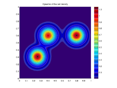
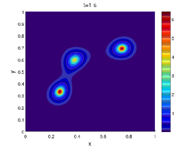
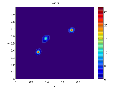
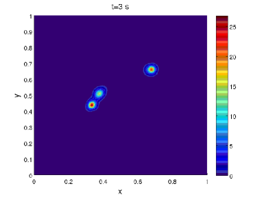
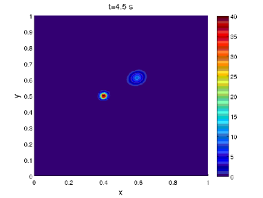
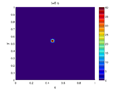
Figure 1: Dynamics of the cell density $\rho$ with intial data given by the sum of three bumps in the case $W_{1}(x)=1-e^{-5|x|}$.

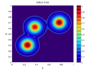
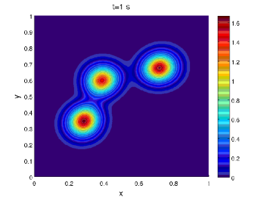
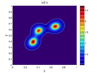
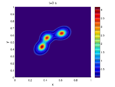
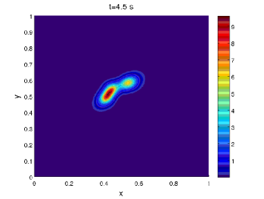
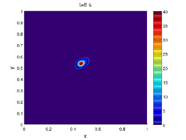
Figure 2: Dynamics of the cell density $\rho$ with intial data given by the sum of three bumps in the case $W_{2}(x)=|x|$.

Due to the finite time collapse result, we expect the convergence in finite time of the solution towards a single Dirac Delta. In fact, this is what we observe in Figure 1 for $W_{1}$ and in Figure 2 for $W_{2}$. However, comparing the two Figures, the qualitative properties of the convergence towards a single Dirac Delta are not the same depending on the choice of the potential.

In fact, within the dynamics given in Figure 1, we can distinguish two phases in the simulation. In a first phase, we notice the concentration of the density into small masses : we can consider that the numerical solution for time $t=1.8\ s$ is a sum of three numerical Dirac masses with small numerical diffusion. Then these three masses aggregate into two and finally one single mass. On the contrary, for the potential $W_{2}$, we observe in Figure 2 that the numerical solution stays regular and bounded until it forms one single bump and then it collapses.

This tends to indicate the existence of two different time scales: the one corresponding to a radial self-similar collapse onto a single Dirac, and the one corresponding to the interactions between different Dirac Deltas. In the case of the potential $W_{1}$, we observe a faster time scale for the self-similar blow-up of regular solutions into several Dirac Deltas, then the trajectories are given by the sticky particle dynamics for these aggregates. Whereas for the potential $W_{2}$ the time scale of the self-similar blow-up is slower compared to the dynamics of the attraction of the aggregates, and then the blow up occurs after all regular bumps aggregate into a single regular bump before the final fate of total collapse.

A very nice feature of this numerical scheme is that it allows for simulations after the first blow-up happens with seemingly good approximation in the measure sense by comparison to the particle simulations, see the one dimensional case [32]. The regularization induced on the Dirac Deltas by the numerical diffusion of the scheme does not seem to change the qualitative properties of the solution.

Appendix

Technical Lemmas

In this appendix we state some technical lemmas which are used in the paper.

Lemma A.1

Let us assume that $W$ satisfies assumptions (A0)–(A2). Let $(\rho_{n})_{n\in\mathbb{N}}$ be a sequence of measures in ${\cal P}_{2}(\mathbb{R}^{d})$ such that $\rho_{n}\rightharpoonup\rho$ weakly as measures. Then

$$\lim_{n\to+\infty}\int_{x\neq y}\nabla W(x-y)\rho_{n}(dy)=\int_{x\neq y}\nabla W(x-y)\rho(dy),\quad\mbox{ for a.e. }x\in\mathbb{R}^{d}.$$

Proof.

We consider a regularization of $W$ by $W_{k}$ with $k\in\mathbb{N}$, $W_{k}\in C^{1}(\mathbb{R}^{d})$, $W_{k}(-x)=W_{k}(x)$, $|\nabla W_{k}|\leq|\nabla W|\leq w_{\infty}$, and

$$\sup_{x\in\mathbb{R}^{d}\setminus B(0,\frac{1}{k})}|\nabla W_{k}(x)-\nabla W(x)|\leq\frac{1}{k}.$$ (A.1)

By definition of the weak convergence of measures, we have

$$\lim_{n\to+\infty}\int_{x\neq y}\nabla W_{k}(x-y)\rho_{n}(dy)=\int_{x\neq y}\nabla W_{k}(x-y)\rho(dy),\quad\mbox{ for a.e. }x\in\mathbb{R}^{d}.$$ (A.2)

In fact, we can remove the point $y=x$ in the integral since by construction $\nabla W_{k}$ is odd, then $\nabla W_{k}(0)=0$. Moreover for all $n\in\mathbb{N}$, we have that

$$\Big{|}\int_{x\neq y}\nabla(W_{k}-W)(x-y)\rho_{n}(dy)\Big{|}\leq \,\Big{|}\int_{B(x,\frac{1}{k})\setminus\{x\}}\nabla(W_{k}-W)(x-y)\rho_{n}(dy)\Big{|}$$

$$+\Big{|}\int_{\mathbb{R}^{d}\setminus B(x,\frac{1}{k})}\nabla(W_{k}-W)(x-y)\rho_{n}(dy)\Big{|}.$$ (A.3)

Given $\varepsilon>0$, we use the property (A.1) to get an estimate on the second term in (A.3)

$$\Big{|}\int_{\mathbb{R}^{d}\setminus B(x,\frac{1}{k})}\nabla(W_{k}-W)(x-y)\rho_{n}(dy)\Big{|}\leq\frac{1}{k}\leq\varepsilon$$ (A.4)

for $k\geq K_{1}$.

Now, we fix $K_{2}\geq K_{1}$ such that

$$\rho\big{(}B(x,\frac{2}{K_{2}})\setminus\{x\}\big{)}\leq\frac{\varepsilon}{4}.$$ (A.5)

We choose a continuous function $0\leq\xi\leq 1$ such that $\xi(x)=1$ on $B(x,\frac{1}{K_{2}})$ and $\xi(x)=0$ on $\mathbb{R}^{d}\setminus B(x,\frac{2}{K_{2}})$. Then $\xi\in C_{c}(\mathbb{R}^{d})$ and for all $k\geq K_{2}$, we have

$$\begin{array}[]{ll}\displaystyle\rho_{n}\big{(}B(x,\frac{1}{k})\setminus\{x\}\big{)}&\displaystyle\leq\rho_{n}\big{(}B(x,\frac{1}{K_{2}})\setminus\{x\}\big{)}\leq\int_{\mathbb{R}^{d}}\xi(x)\rho_{n}(dx)\\[8.53581pt] &\displaystyle\leq\int_{\mathbb{R}^{d}}\xi(x)(\rho_{n}-\rho)(dx)+\frac{\varepsilon}{4},\end{array}$$

where we use (A.5) for the last inequality. From the weak convergence as measures of $\rho_{n}$ towards $\rho$, we have that for $n\geq N_{1}$ large enough

$$\Big{|}\int_{\mathbb{R}^{d}}\xi(x)(\rho_{n}-\rho)(dx)\Big{|}\leq\frac{\varepsilon}{4}.$$

Thus, for $k\geq K_{2}$ we obtain

$$\rho_{n}\big{(}B(x,\frac{1}{k})\setminus\{x\}\big{)}\leq\frac{\varepsilon}{2}\,,$$

uniform in $n\geq N_{1}$. Therefore, we can bound the first term of the right hand side in (A.3) as

$$\Big{|}\int_{B(x,\frac{1}{k})\setminus\{x\}}\nabla(W_{k}-W)(x-y)\rho_{n}(dy)\Big{|}\leq 2w_{\infty}\rho_{n}(B(x,\frac{1}{k})\setminus\{x\})\leq w_{\infty}\varepsilon\,.$$

Collecting the last inequality with (A.4), we deduce that

$$\lim_{k\to\infty}\int_{x\neq y}\nabla W_{k}(x-y)\rho_{n}(dy)=\int_{x\neq y}\nabla W(x-y)\rho_{n}(dy),$$

uniformly for $n\geq N_{1}$. The same argument shows in particular that

$$\lim_{k\to\infty}\int_{x\neq y}\nabla W_{k}(x-y)\rho(dy)=\int_{x\neq y}\nabla W(x-y)\rho(dy).$$

We conclude by passing into the limit $k\to\infty$ in (A.2).

Lemma A.2

Let us assume that $W$ satisfies assumptions (A0)–(A2). Let $(W_{n})_{n\in\mathbb{N}^{*}}$ be a sequence of even functions in $C^{1}(\mathbb{R}^{d})$ satisfying (A1) and (1.2) with constants $\lambda$ and $w_{\infty}$ not depending on $n$ and such that

$$sup_{x\in\mathbb{R}^{d}\setminus B(0,\frac{1}{n})}\big{|}\nabla W_{n}(x)-\nabla W(x)\big{|}\leq\frac{1}{n},\qquad\mbox{ for all }n\in\mathbb{N}^{*}.$$ (A.6)

Let $(\rho_{n})_{n\in\mathbb{N}}$ be a sequence of measures in ${\cal P}_{2}(\mathbb{R}^{d})$ such that $\rho_{n}\rightharpoonup\rho$ tightly. Then we have

$$\lim_{n\to+\infty}\int_{\mathbb{R}^{d}}\nabla W_{n}(x-y)\rho_{n}(dy)=\int_{x\neq y}\nabla W(x-y)\rho(dy),\quad\mbox{ for a.e. }x\in\mathbb{R}^{d}.$$

Proof.

Let us denote by

$$a_{n}(x):=-\int_{\mathbb{R}^{d}}\nabla W_{n}(x-y)\rho_{n}(dy),\quad\mbox{ and }a(x):=-\int_{x\neq y}\nabla W(x-y)\rho(dy).$$

We notice that since $W_{n}$ is even, we have $\nabla W_{n}(0)=0$, then

$$a_{n}(x):=-\int_{x\neq y}\nabla W_{n}(x-y)\rho_{n}(dy).$$

Let $\varepsilon>0$, from Lemma A.1 we deduce that there exists $N_{1}\in\mathbb{N}^{*}$ such that for all $n\geq N_{1}$,

$$\Big{|}\int_{x\neq y}\nabla W(x-y)(\rho_{n}-\rho)(dy)\Big{|}\leq\frac{\varepsilon}{4}.$$ (A.7)

Then using (A.6), we deduce that

$$\Big{|}\int_{x\neq y}\big{(}\nabla W_{n}(x-y)-\nabla W(x-y)\big{)}\rho_{n}(dy)\Big{|}\leq\frac{1}{n}+\int_{B(x,\frac{1}{n})\setminus\{x\}}\big{|}\nabla W_{n}(x-y)-\nabla W(x-y)\big{|}\rho_{n}(dy).$$ (A.8)

Now, we proceed as in the proof of Lemma A.1. From assumptions on $W_{n}$ and $W$, we deduce (see (1.2)) that there exists a constant $C$ such that

$$\int_{B(x,\frac{1}{n})\setminus\{x\}}\big{|}\nabla W_{n}(x-y)-\nabla W(x-y)\big{|}\rho_{n}(dy)\leq C\rho_{n}\big{(}B(x,\frac{1}{n})\setminus\{x\}\big{)}$$ (A.9)

We fix $N_{2}\geq N_{1}$ such that

$$\rho\big{(}B(x,\frac{2}{N_{2}})\setminus\{x\}\big{)}\leq\frac{\varepsilon}{4}.$$ (A.10)

We choose a continuous function $0\leq\xi\leq 1$ such that $\xi(x)=1$ on $B(x,\frac{1}{N_{2}})$ and $\xi(x)=0$ on $\mathbb{R}^{d}\setminus B(x,\frac{2}{N_{2}})$. Then $\xi\in C_{c}(\mathbb{R}^{d})$ and for all $n\geq N_{2}$, we have

$$\begin{array}[]{ll}\displaystyle\rho_{n}\big{(}B(x,\frac{1}{n})\setminus\{x\}\big{)}&\displaystyle\leq\rho_{n}\big{(}B(x,\frac{1}{N_{2}})\setminus\{x\}\big{)}\leq\int_{\mathbb{R}^{d}}\xi(x)\rho_{n}(dx)\\[8.53581pt] &\displaystyle\leq\int_{\mathbb{R}^{d}}\xi(x)(\rho_{n}-\rho)(dx)+\frac{\varepsilon}{4},\end{array}$$

where we use (A.10) for the last inequality. From the tight convergence of $\rho_{n}$ towards $\rho$, we have that for $n\geq N_{3}$ large enough (and $N_{3}>N_{2}$),

$$\Big{|}\int_{\mathbb{R}^{d}}\xi(x)(\rho_{n}-\rho)(dx)\Big{|}\leq\frac{\varepsilon}{4}.$$

Thus, for $n\geq N_{3}$

$$\rho_{n}\big{(}B(x,\frac{1}{n})\setminus\{x\}\big{)}\leq\frac{\varepsilon}{2}.$$

Plugging this latter inequality into (A.9) and from (A.8), we deduce that for $n\geq N_{3}$,

$$\Big{|}\int_{x\neq y}\big{(}\nabla W_{n}(x-y)-\nabla W(x-y)\big{)}\rho_{n}(dy)\Big{|}\leq\frac{1}{n}+C\frac{\varepsilon}{2}$$

Finally, combining this latter inequality with (A.7), we deduce that for $n\geq N_{3}$,

$$\big{|}a_{n}(x)-a(x)|\leq\frac{\varepsilon}{4}+\frac{1}{n}+C\frac{\varepsilon}{2},\qquad\mbox{for a.e. }x\in\mathbb{R}^{d}.$$

Acknowledgements. JAC acknowledges support from projects MTM2011-27739-C04-02, 2009-SGR-345 from Agència de Gestió d’Ajuts Universitaris i de Recerca-Generalitat de Catalunya, the Royal Society through a Wolfson Research Merit Award, and the Engineering and Physical Sciences Research Council (UK) grant number EP/K008404/1. NV acknowledges partial support from the french ”ANR blanche” project Kibord : ANR-13-BS01-0004.

References

- [1] L. Ambrosio, N. Gigli, G. Savaré, Gradient flows in metric space of probability measures, Lectures in Mathematics, Birkäuser, 2005
- [2] J-P. Aubin, A. Cellina, Differential inclusions. Set-valued maps and viability theory. Grundlehren der Mathematischen Wissenschaften [Fundamental Principles of Mathematical Sciences], 264. Springer-Verlag, Berlin, 1984.
- [3] D. Balagué, J. A. Carrillo, T. Laurent, G. Raoul, Dimensionality of local minimizers of the interaction energy, Arch. Ration. Mech. Anal. 209 (2013), no. 3, 1055–1088.
- [4] D. Benedetto, E. Caglioti, M. Pulvirenti, A kinetic equation for granular media, RAIRO Model. Math. Anal. Numer., 31 (1997), 615-641.
- [5] A. L. Bertozzi, J. von Brecht, H. Sun, T. Kolokolnikov, D. Uminsky, Ring Patterns and their Bifurcations in a Nonlocal Model of Biological Swarms, to appear in Comm. Math. Sci.
- [6] A.L. Bertozzi, J.A. Carrillo, T. Laurent, Blow-up in multidimensional aggregation equation with mildly singular interaction kernels, Nonlinearity 22 (2009), 683-710.
- [7] A.L. Bertozzi, T. Laurent, J. Rosado, theory for the multidimensional aggregation equation, Comm. Pure Appl. Math., 64(1) (2011) 45–83.
- [8] S. Bianchini, M. Gloyer, An estimate on the flow generated by monotone operators, Comm. Partial Diff. Eq., 36 (2011), no 5, 777–796.
- [9] M. Bodnar, J. J. L. Velázquez, An integro-differential equation arising as a limit of individual cell-based models, J. Differential Equations 222 (2006), no. 2, 341–380.
- [10] G.A. Bonaschi, J.A. Carrillo, M. Di Francesco, M.A. Peletier, Equivalence of gradient flows and entropy solutions for singular nonlocal interaction equations in 1D, arXiv:1310.4110
- [11] F. Bouchut, F. James, One-dimensional transport equations with discontinuous coefficients, Nonlinear Analysis TMA, 32 (1998), no 7, 891–933.
- [12] F. Bouchut, F. James, Duality solutions for pressureless gases, monotone scalar conservation laws, and uniqueness, Comm. Partial Differential Eq., 24 (1999), 2173–2189.
- [13] J. von Brecht, D. Uminsky, On soccer balls and linearized inverse statistical mechanics, J. Nonlinear Sci. 22 (2012), no. 6, 935–959.
- [14] J. von Brecht, D. Uminsky, T. Kolokolnikov, A. L. Bertozzi, Predicting pattern formation in particle interactions, Math. Models Methods Appl. Sci. 22 (2012), suppl. 1, 1140002.
- [15] J. A. Carrillo, A. Chertock, Y. Huang, A Finite-Volume Method for Nonlinear Nonlocal Equations with a Gradient Flow Structure, to appear in Comm. in Comp. Phys.
- [16] J. A. Carrillo, M. DiFrancesco, A. Figalli, T. Laurent, D. Slepčev, Global-in-time weak measure solutions and finite-time aggregation for nonlocal interaction equations, Duke Math. J. 156 (2011), 229–271.
- [17] J. A. Carrillo, S. Lisini, E. Mainini, Gradient flows for non-smooth interaction potentials. Nonlinear Anal. 100 (2014), 122–147.
- [18] J. A. Carrillo, R. J. McCann, C. Villani, Contractions in the 2-Wasserstein length space and thermalization of granular media, Arch. Rational Mech. Anal. 179 (2006), 217–263.
- [19] J. A. Carrillo, J. Rosado, Uniqueness of bounded solutions to aggregation equations by optimal transport methods. European Congress of Mathematics, 3–16, Eur. Math. Soc., Zürich, 2010.
- [20] R.M. Colombo, M. Garavello, M. Lécureux-Mercier, A class of nonlocal models for pedestrian traffic, Math. Models Methods Appl. Sci., (2012) 22(4):1150023, 34.
- [21] K. Craig, A. L. Bertozzi, A blob method for the aggregation equation, preprint.
- [22] G. Crippa, M. Lécureux-Mercier, Existence and uniqueness of measure solutions for a system of continuity equations with non-local flow, NoDEA Nonlinear Differential Equations Appl., (2013) 20 (3):523–537.
- [23] M. Di Francesco, S. Fagioli, Measure solutions for non-local interaction PDEs with two species, Nonlinearity 26 (2013), 2777–2808.
- [24] J. Dolbeault, C. Schmeiser, The two-dimensional Keller-Segel model after blow-up, Disc. Cont. Dyn. Syst. A 25 (2009), 109–121.
- [25] Y. Dolak, C. Schmeiser, Kinetic models for chemotaxis: Hydrodynamic limits and spatio-temporal mechanisms, J. Math. Biol., 51 (2005), 595–615.
- [26] F. Filbet, Ph. Laurençot, B. Perthame, Derivation of hyperbolic models for chemosensitive movement, J. Math. Biol., 50 (2005), 189–207.
- [27] A.F. Filippov, Differential Equations with Discontinuous Right-Hand Side, A.M.S. Transl. (2) 42 (1964), 199–231.
- [28] Y. Huang, A. L. Bertozzi, Asymptotics of blowup solutions for the aggregation equation, Discrete and Continuous Dynamical Systems - Series B, 17 2012, 1309–1331.
- [29] Y. Huang, A. L. Bertozzi, Self-similar blowup solutions to an aggregation equation in , SIAM Journal on Applied Mathematics, 70 2010, 2582–2603.
- [30] F. James, N. Vauchelet, Chemotaxis: from kinetic equations to aggregation dynamics, Nonlinear Diff. Eq. and Appl. (NoDEA), 20 (2013), no 1, 101–127.
- [31] F. James, N. Vauchelet, Equivalence between duality and gradient flow solutions for one-dimensional aggregation equations, preprint http://hal.archives-ouvertes.fr/hal-00803709, submitted.
- [32] F. James, N. Vauchelet, Numerical method for one-dimensional aggregation equations, preprint http://hal.archives-ouvertes.fr/hal-00803709, submitted.
- [33] E.F. Keller, L.A. Segel, Initiation of slime mold aggregation viewed as an instability, J. Theor. Biol., 26 (1970), 399–415.
- [34] H. Li, G. Toscani, Long time asymptotics of kinetic models of granular flows, Arch. Rat. Mech. Anal., 172 (2004), 407–428.
- [35] G. Loeper, Uniqueness of the solution to the Vlasov-Poisson system with bounded density. J. Math. Pures Appl. (9) 86 (2006), no. 1, 68–79.
- [36] S. Luckhaus, Y. Sugiyama, J. J. L. Velázquez, Measure valued solutions of the 2D Keller-Segel system, Arch. Rational Mech. Anal. 206 (2012), 31–80.
- [37] D. Morale, V. Capasso, K. Oelschläger, An interacting particle system modelling aggregation behavior: from individuals to populations, J. Math. Biol., 50 (2005), 49–66.
- [38] A. Okubo, S. Levin, Diffusion and Ecological Problems: Modern Perspectives, Springer, Berlin, 2002.
- [39] C.S. Patlak, Random walk with persistence and external bias, Bull. Math. Biophys., 15 (1953), 311-338.
- [40] B. Perthame, C. Schmeiser, M. Tang, N. Vauchelet, Traveling plateaus for a hyperbolic Keller-Segel system with attraction and repulsion: existence and branching instabilities, Nonlinearity 24 (2011) 1253–1270.
- [41] F. Poupaud, Diagonal defect measures, adhesion dynamics and Euler equation, Methods Appl. Anal., 9 (2002), no 4, 533–561.
- [42] F. Poupaud, M. Rascle, Measure solutions to the linear multidimensional transport equation with discontinuous coefficients, Comm. Partial Diff. Equ., 22 (1997), 337–358.
- [43] C. M. Topaz, A. L. Bertozzi, Swarming patterns in a two-dimensional kinematic model for biological groups, SIAM J. Appl. Math. 65 (2004), 152–174.
- [44] G. Toscani, Kinetic and hydrodynamic models of nearly elastic granular flows, Monatsh. Math. 142, 179–192.
- [45] C. Villani, Optimal transport, old and new, Grundlehren der Mathematischen Wissenschaften 338, Springer, 2009.
- [46] C. Villani, Topics in optimal transportation, Graduate Studies in Mathematics 58, Amer. Math. Soc, Providence, 2003.