The stability of extended Floater-Hormann interpolants

Abstract

We present a new analysis of the stability of extended Floater-Hormann interpolants, in which both noisy data and rounding errors are considered. Contrary to what is claimed in the current literature, we show that the Lebesgue constant of these interpolants can grow exponentially with the parameters that define them, and we emphasize the importance of using the proper interpretation of the Lebesgue constant in order to estimate correctly the effects of noise and rounding errors. We also present a simple condition that implies the backward instability of the barycentric formula used to implement extended interpolants. Our experiments show that extended interpolants mentioned in the literature satisfy this condition and, therefore, the formula used to implement them is not backward stable. Finally, we explain that the extrapolation step is a significant source of numerical instability for extended interpolants based on extrapolation.

1 Introduction

Given nodes $\mathbf{x}=\left(x_{0},\dots,x_{n}\right)$, an integer $\delta$ with $0\leq\delta\leq n$ and function values $\mathbf{y}=\left(y_{0},\dots,y_{n}\right)$, the Floater-Hormann interpolation formula is defined as

$${r_{\delta}}\!\left(t,\mathbf{x},\mathbf{y}\right):=\frac{\sum_{i=0}^{n-\delta}{\lambda_{i}}\!\left(t,\mathbf{x}\right){p_{i}}\!\left(t,\mathbf{x},\mathbf{y}\right)}{\sum_{i=0}^{n-\delta}{\lambda_{i}}\!\left(t,\mathbf{x}\right)},$$ (1)

where ${p_{i}}\!\left(t,\mathbf{x},\mathbf{y}\right)$ is the unique polynomial of degree at most $\delta$ which interpolates $y_{i},y_{i+1},\dots,y_{i+\delta}$ at $x_{i},x_{i+1},\dots,x_{i+\delta}$, and the weights $\lambda_{i}$ are defined as

$${\lambda_{i}}\!\left(t,\mathbf{x}\right):=\frac{\left(-1\right)^{i}}{\left(t-x_{i}\right)\left(t-x_{i+1}\right)\dots\left(t-x_{i+\delta}\right)},\hskip 28.45274pt\mathrm{for}\ i=0,\dots,n-\delta.$$

In exact arithmetic, when $y_{i}={f}\!\left(x_{i}\right)$ for a smooth function $f$, the error incurred by the Floater-Hormann interpolant defined by $\mathbf{x}$ and $\delta$ is of order $h^{\delta+1}$, where

$$h:=\max_{0\leq k<n}x_{k+1}-x_{k}.$$

Unfortunately, when the nodes are equally spaced the Lebesgue constant of the Floater-Hormann interpolant defined by $\mathbf{x}$ and $\delta$ grows exponentially with $\delta$ (see Bos ). Therefore, $\delta$ must be chosen carefully in order to balance the high order of approximation $h^{\delta+1}$ with the numerical errors due to large Lebesgue constants.

In an attempt to reduce the effects of the large Lebesgue constants for equally spaced nodes, Klein Klein introduced the extended Floater-Hormann interpolants. These interpolants are defined in terms of an integer parameter $d\geq 0$, extended nodes $\tilde{x}_{-d},\tilde{x}_{1-d},\dots,\tilde{x}_{0},\dots\tilde{x}_{n},\dots,\tilde{x}_{n+d}$, with $\tilde{x}_{i}=x_{0}+ih$, and extended function values $\tilde{y}_{-d},\dots\tilde{y}_{0},\dots\tilde{y}_{n},\dots\tilde{y}_{n+d}$. Each

$$\tilde{\mathbf{y}}={Y}\!\left(d,\mathbf{x},\mathbf{y}\right)\in{\mathds{R}}^{n+2d+1}$$

in combination with $r_{d}$ in (1) leads to an extended interpolant given by

$${\tilde{r}_{d,Y}}\!\left(t,\mathbf{x},\mathbf{y}\right):={r_{d}}\!\left(t,\tilde{\mathbf{x}},{Y}\!\left(d,\mathbf{x},\mathbf{y}\right)\right).$$ (2)

The choice of the extended function values is a crucial point regarding the stability and accuracy of the extended interpolants. Usually, we do not have information outside of the interpolation interval and in practice the $\tilde{y}$ must be estimated, and they will not be exact. To the best of our knowledge, the only concrete way for choosing the $\tilde{y}$ mentioned in the literature prior to our writing of this article is the one outlined in the fifth page of Klein and Berrut BerrutKleinCAM , which is based on two additional parameters $\tilde{d}$ and $\tilde{n}$:

“More precisely, $2d$ extra nodes $x_{-d},\dots,x_{-1}$ are considered, $d$ on each side of the interval, and approximate values $\tilde{f}_{i}$ of $f$ at these nodes are computed by a discrete Taylor polynomial with derivatives approximated by (linear rational) finite differences (see Section 8) using only the given values of $f$ in $[a,b]$. These finite differences are the derivatives of the Floater-Hormann family with parameters $\tilde{d}$ in the nodes $x_{0},\dots,x_{\tilde{n}}$, resp. $x_{n-\tilde{n}},\dots,x_{n}$, for an $\tilde{n}$ much smaller than $n$. At the original nodes, $x_{j}$, $j=0,\dots,n$, the given $f_{f}$ are used.”

Klein Klein shows that the order of approximation of the extended interpolant above is $h^{\mu+1}$, where $\mu:=\min\{d,\tilde{d}\}$. Usual Floater-Hormann interpolants have order of approximation $\delta$, and $\mu$ is the analogous to the parameter $\delta$ used to define usual Floater-Hormann interpolants. Therefore, it is important to distinguish $\delta$ from $d$. In fact, when choosing the parameters in practice, one must be aware that the order of approximation $\mu$ will be unaffected by increasing the parameter $d$ once this parameter is already larger than $\tilde{d}$. This argument and our practical experience with extended interpolants suggest that as first choice one should pick $d=\tilde{d}=\delta$ (see also Fig. 1 below.) For this reasons, our theory pays special attention to the case $d=\delta$, but we do address more general cases in our experiments.

The articles Klein and Berrut BerrutKleinCAM and Klein Klein also claim that the Lebesgue constant of Klein’s extended Floater-Hormann interpolant grows logarithmically with $n$ and $d$, regardless of $\tilde{n}$ and $\tilde{d}$. Theorem 5.1 in page 6 of BerrutKleinCAM summarizes this and other claims from Klein (see, in particular, Theorems 2.1 and 3.1 of Klein and the remark following the latter.) We cite:

Theorem 5.1(from BerrutKleinCAM ) Suppose $n$, $d$, $\tilde{n}$ and $\tilde{d}$ are positive integers, $\tilde{d}\leq\tilde{n}<n$ and assume that $f\in C^{d+2}[a-dh,d+dh]\cap{C^{2d+1}}\!\left([a,a+\tilde{n}h]\cup[b-\tilde{n}h,b]\right)$ is sampled at $n+1$ equispaced nodes in $[a,b]$. Then

• $\tilde{r}_{n}[f]$ has no real poles;

• For a constant $K$ independent of $n$, $\left\|{\tilde{r}_{n}[f]-f}\right\|\leq Kh^{\min{\left\{d,\tilde{d}\right\}}+1}$;

• The associated Lebesgue constant $\tilde{\Lambda}_{n}$ grows logarithmically with $n$ and $d$:

  $$\tilde{\Lambda}_{n}\leq 2+{\ln}\!\left(n+2d\right).$$

Here we show that, in general, the third item in this theorem is false if, as in page 2 of Berrut and Klein BerrutKleinCAM , we assume the standard definition of the Lebesgue constant as the norm of the interpolation operator, and take into account the unavoidable errors in the extended function values $\tilde{y}$. We prove that the traditional Lebesgue constant grows exponentially with $d$ when $d=\tilde{n}=\tilde{d}$ and $\tilde{\mathbf{y}}$ is outlined in BerrutKleinCAM . In the version of Theorem 5.1 stated in Klein Klein the reader is informed that actually the logarithmic bound assumes a peculiar interpretation of the Lebesgue constant, namely, essentially that the mentioned approximate function values have no errors; see the paragraph above Theorem 3.1 in Klein . However, this limitation of the result (iii) is not mentioned in BerrutKleinCAM , and neither BerrutKleinCAM nor Klein point out that the theorem does not apply to the choices of $\tilde{\mathbf{y}}$ proposed for the extended Floater-Hormann interpolants and used in the experiments.

Rigorously, our proof applies only to the case $d=\tilde{d}=\tilde{n}$. It suffices as a counterexample to Theorem 5.1, but it is unsatisfactory from a broader practical perspective. However, we emphasize that, in practice, Theorem 5.1 gives a misleading impression regarding the Lebesgue constant of Extended Floater-Hormann interpolants for broader classes of parameters. We do not have a formal theory supporting this claim, but Sections 2 and 3 and Figure 1 below present strong experimental evidence of its validity.

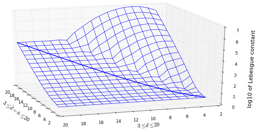
Figure 1: Log10 of the correct Lebesgue constant as a function of $3\leq d,\tilde{d}\leq 20$, for $n=100$ and $\tilde{n}=\tilde{d}$. Note that the diagonal $d=\tilde{d}$ highlighted in this figure crosses the lines of constant $\tilde{d}$ in places in which the Lebesgue constant is near the minimal value along such lines. Therefore, it makes little sense to choose $d$ much less than $\tilde{d}$, and the case considered in our counterexample is quite relevant in practice. We have observed similar pictures for other values of $n$ and our experiments indicate that the Lebesgue constant increases as $\tilde{n}$ gets larger than $\tilde{d}$.

This article presents an stability analysis of extended Floater-Hormann interpolants based on the appropriate interpretation of the Lebesgue constant. Formally, when the function $Y$ which yields the extended function values $\tilde{\mathbf{y}}$ is linear in $\mathbf{y}$, we consider the linear operator $\mathbf{y}\mapsto r_{\mathbf{x},d,Y}[\mathbf{y}]\in C^{0}[a,b]$ given by

$${r_{\mathbf{x},d,Y}[\mathbf{y}]}\!\left(t\right):={\tilde{r}_{d,Y}}\!\left(t,\mathbf{x},\mathbf{y}\right),$$

for $\tilde{r}_{d,Y}$ defined in (2), and the Lebesgue constant can be defined either as the norm of this linear operator with respect to the supremum norm in ${\mathds{R}}^{n+1}$ and $C^{0}[x_{0},x_{n}]$, or as the supremum of the Lebesgue function

$${\Lambda_{\mathbf{x},d,Y}}\!\left(t\right):=\sup_{\mathbf{y}\ \mathrm{with}\ \left\|{\mathbf{y}}\right\|_{\infty}=1}\left|{r_{\mathbf{x},d,Y}[\mathbf{y}]}\!\left(t\right)\right|$$ (3)

in $[x_{0},x_{n}]$. These two definitions are equivalent, and lead to a concept which has a fundamental role in theory and in practice, provided that it is interpreted correctly.

By considering the correct Lebesgue constant, we gain a more realistic view of the stability of extended Floater-Hormann interpolants. For instance, we learn that the version of these interpolants mentioned in Klein and Berrut BerrutKleinCAM and Klein Klein should not be used with large $\tilde{d}$. Since the order of approximation of these interpolants is $h^{\mu}$ for $\mu=\min{\left\{d,\tilde{d}\right\}}$, this limits their accuracy in practice.

The articles BerrutKleinCAM and Klein say nothing about the disastrous effect that a large $\tilde{d}$ may have on extended interpolants. Instead, they emphasize that these interpolants can be used with large $d$. This is illustrated by Figures 6 in BerrutKleinCAM and Klein , which explore only the case $\tilde{d}=7$ and compare the resulting extended interpolants with usual interpolants with $d=\delta$ as large as $50$. If instead of considering $d=\delta$ as large as 50 in their Figure 6, they had focused on the more modest case $1\leq d=\delta\leq\tilde{d}=7$, as in their other experiments, then they would have a more realistic argument in favor of extended interpolants. Indeed, for this range of $d=\delta$, Figures 5 to 10 in Klein show that extended interpolants are better than usual ones in cases of practical interest. Therefore, extended interpolants have merit and are a relevant topic for research. However, our experiments in Section 6 show that there are also cases in which extended interpolants are worse than usual ones, and here we aim at a balanced view of their properties and limitations. In particular, we discuss the role played by each one of their parameters and the ranges in which they should be used.

In sections 3 and 4 we analyze the Lebesgue constants of extended interpolants from a theoretical perspective. We present an exponential lower bound on the Lebesgue constant when $d=\tilde{n}=\tilde{d}$. We also present experimental data showing that the dependency of the Lebesgue function on these three parameters is not accurately described by Theorem 5.1 in more general settings. Section 5 discusses the backward stability of extended Floater-Hormann interpolants in the general case in which the function ${Y}\!\left(d,\mathbf{x},\mathbf{y}\right)$ that defines $\tilde{\mathbf{y}}$ is linear in $\mathbf{y}$. We present a simple condition that implies the backward instability of the barycentric formula used to implement extended interpolants in this case, and we show experimentally that this condition for backward instability is satisfied by an extended interpolant mentioned in Klein .

Section 6 presents an empirical analysis of the stability of the extended interpolants outlined in Berrut and Klein BerrutKleinCAM . We explain that the extrapolation step may lead to numerical instability, and due to this instability the overall error incurred by these interpolants can be much larger than $\epsilon n\tilde{\Lambda}_{\mathbf{x},d,Y}{}\,\left\|{\mathbf{y}}\right\|_{\infty}$, where $\tilde{\Lambda}_{\mathbf{x},d,Y}{}$ is its Lebesgue constant and $\epsilon$ is the machine precision. In order to illustrate this fact, we present the results of experiments in which the accuracy of the extended interpolants is much worse than the accuracy of the usual interpolants.

On the positive side, once we become aware of the problems caused by the extrapolation step, we may consider ways to reduce them. When evaluating the interpolants for many values of $t\in[x_{0},x_{n}]$, it is worth computing the relatively few extrapolated function values in multiple precision. Numerical experiments show that this strategy leads to more accurate extended interpolants.

Finally, the appendix considers the difficulties involved in the construction of a general stability theory for extended interpolants. This appendix is at a more abstract level than the rest of the article: we argue about the arguments one would use to discuss the stability of extended interpolants. We hope that people interested in an in depth analysis of the stability of these interpolants will appreciate our remarks regarding the difficulties in formulating realistic hypotheses and theorems about this subject.

2 The rounding errors and the Lebesgue constant in practice

The Lebesgue constant is a fundamental concept in approximation theory. It is also fundamental in practice, because it measures the sensitivity of the interpolants to perturbations (or noise) in the data. In its proper interpretation, the Lebesgue constant is equivalent to what numerical analysts call condition number, and use to evaluate the numerical stability of algorithms.

This section shows that that rounding errors and noisy data have devastating effects on interpolants for which theorems in BerrutKleinCAM and Klein claim that the Lebesgue constant is small. Therefore, such claims may lead readers to believe that these interpolants are much less affected by noise and rounding errors than they really are. Figure 2 considers the approximation of ${f}\!\left(t\right)={\sin}\!\left(2t\right)$ for $t\in[-1,1]$. The plot on the left of Figure 2 shows that by implementing the extrapolation procedure proposed in BerrutKleinCAM and Klein with the usual IEEE 754 double precision arithmetic we may have numerical errors of order $10^{14}$ in circumstances in which Theorem 5.1 yields a bound smaller than $8$ on the constant which Berrut and Klein call by Lebesgue’s name. These errors are several orders of magnitude larger than the ones reported in BerrutKleinCAM and Klein for the same kind of extended interpolant, because we do not restrict ourselves to the same small values of $\tilde{d}$ as BerrutKleinCAM and Klein .

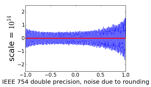
(a)

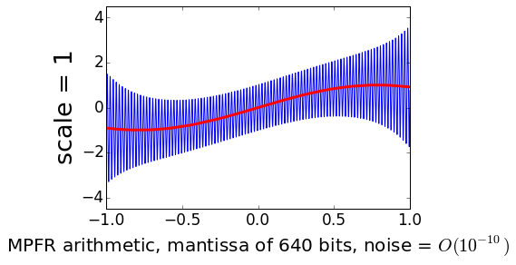
(b)

Figure 2: The function ${f}\!\left(t\right)={\sin}\!\left(2t\right)$ (in red) and the approximation obtained following the procedure proposed in BerrutKleinCAM with $n=200$ (in blue). We use $d=\tilde{n}=\tilde{d}=40$, whereas BerrutKleinCAM and Klein consider $0\leq d\leq 50$ and smaller values of $\tilde{n}$ and $\tilde{d}$ in their experiments. The $\tilde{d}$ and $\tilde{n}$ in this figure satisfy the hypothesis of Theorem 5.1 and $d$ is within the range considered in the experiments in BerrutKleinCAM and Klein .

The plot on the right of Figure 2 illustrates the sensitivity of extended interpolants to noise in the function values. It was obtained by adding random values of order $10^{-10}$ to $y_{0},\dots,y_{n}$. The effects of rounding errors in this plot are negligible because we used the high precision arithmetic provided by the MPFR library MPFR , with a mantissa of 640 bits. The experiment on the right indicates that in this case the condition number is about $10^{10}$, and not $8$ as suggested by Theorem 5.1 of Berrut and Klein BerrutKleinCAM .

Figure 2 raises an interesting question: why does the plot on the left display errors of order $10^{14}$ while the plot on the right shows errors of order one? This question is intriguing because the IEEE 754’s double precision machine epsilon is of order $10^{-16}$ and is much smaller than the ${O}\!\left(10^{-10}\right)$ perturbations used to generate the plot on the right. As we explain in the rest of the article, the answer to this question lies in the instabilities in the extrapolation process proposed by Klein Klein and this is one more reason why, in practice, the logarithmic bound presented in BerrutKleinCAM and Klein underestimates the effects of noise and rounding errors.

3 The barycentric and reduced forms and the Lebesgue function

In this section we show how to write extended interpolants in barycentric form and introduce another way to describe them, which we call reduced form. This form is numerically unstable and we do not advocate its use in practice. Its purpose is to help us to deduce an expression for the Lebesgue function of extended interpolants.

The Lebesgue function measures the sensitivity of the output of the complete interpolation process to perturbations in its input, and we emphasize that the input to the interpolation process are the original function values $y_{i}$; not the extrapolated function values $\tilde{y}_{i}$. Therefore, we can not ignore how changes in $\mathbf{y}$ affect $\mathbf{\tilde{y}}$ as suggested by Equation (3.2) in Klein .

We recall that extended Floater-Hormann interpolants are defined only for equally spaced nodes, and in this section focus on the interpolants with $\tilde{\mathbf{y}}$ as in the fifth section of BerrutKleinCAM , ie., $\tilde{\mathbf{y}}$ is defined using extrapolation. When the nodes are equally spaced, Floater shows that usual Floater-Hormann interpolants can be written in the barycentric form

$${r_{\mathbf{x},\delta}[\mathbf{y}]}\!\left(t\right)=\ \ \left.\sum\limits_{i=0}^{n}\frac{w_{n,\delta,i}\,y_{i}}{t-x_{i}}\right/\sum\limits_{i=0}^{n}\frac{w_{n,\delta,i}}{t-x_{i}},$$ (4)

with weights

$$w_{n,\delta,i}=(-1)^{i-\delta}\sum_{j=\max\{0,\,i-\delta\}}^{\min\{n-\delta,\,i\}}\left(\begin{array}[]{c}\delta\\ i-j\end{array}\right),$$ (5)

where the $y_{i}$ are the interpolated function values. In the last paragraph of page 5 of BerrutKleinCAM , extended interpolants are defined by extrapolating $\mathbf{y}$ according to the following Taylor series, which are defined in terms of the parameters $\tilde{d}$ and $\tilde{n}$:

$$\tilde{y}_{i} := y_{0}+\sum_{k=1}^{\tilde{d}}{r_{\underline{\mathbf{x}},\tilde{d}}^{(k)}[\underline{\mathbf{y}}]}\!\left(x_{0}\right)\frac{\left(\tilde{x}_{i}-x_{0}\right)^{k}}{k!}\ \hskip 42.67912pt\mathrm{for}\ -d\leq i<0,$$ (6)

$$\tilde{y}_{i} := y_{i}\hskip 165.59525pt\mathrm{for}\ 0\leq i\leq n,$$ (7)

$$\tilde{y}_{i} := y_{n}+\sum_{k=1}^{\tilde{d}}{r_{\overline{\mathbf{x}},\tilde{d}}^{(k)}[\overline{\mathbf{y}}]}\!\left(x_{n}\right)\frac{\left(\tilde{x}_{i}-x_{n}\right)^{k}}{k!}\ \hskip 39.83368pt\mathrm{for}\ n<i\leq n+d,$$ (8)

where $\tilde{x}_{i}=x_{0}+ih$ for $-d\leq i\leq n+d$ and ${r^{(k)}_{\mathbf{x},d}[\mathbf{y}]}\!\left(t\right)$ is the $k$th derivative of the Floater-Hormann interpolant ${r_{\mathbf{x},d}[\mathbf{y}]}\!\left(t\right)$ in (4) and $\underline{\mathbf{x}}:=\left(x_{0},\dots,x_{\tilde{n}}\right)$, $\underline{\mathbf{y}}:=\left(y_{0},\dots,y_{\tilde{n}}\right)$, $\overline{\mathbf{x}}:=\left(x_{n-\tilde{n}},\dots,x_{n}\right)$ and $\overline{\mathbf{y}}:=\left(y_{n-\tilde{n}},\dots,y_{n}\right)$. Therefore, the extended interpolant is specified once we define $\mathbf{x}$, $d$, $\tilde{n}$ and $\tilde{d}$, and we can write it in the following barycentric form:

$${\tilde{r}_{\mathbf{x},d,\tilde{n},\tilde{d}}[\mathbf{y}]}\!\left(t\right)=\ \ \left.\sum\limits_{i=-d}^{n+d}\frac{\tilde{w}_{n,d,i}\,\tilde{y}_{i}}{t-\tilde{x}_{i}}\right/\sum\limits_{i=-d}^{n+d}\frac{\tilde{w}_{n,d,i}}{t-\tilde{x}_{i}},$$ (9)

with weights

$$\tilde{w}_{n,d,i}:=w_{n+2d,d,i+d}=(-1)^{i}\sum_{j=\max\{0,\,i\}}^{\min\{n+d,\,i+d\}}\left(\begin{array}[]{c}d\\ i+d-j\end{array}\right).$$

It is difficult to derive the Lebesgue function of the extended interpolant $\tilde{r}_{\mathbf{x},d,\tilde{n},\tilde{d}}{}$ directly from Equation (9), because this equation depends on $\tilde{\mathbf{y}}$, which is not part of the original interpolation problem. To derive an expression for this Lebesgue function, it is helpful to write the extended interpolant only in terms of the original $\mathbf{y}$. The next lemma explains how to achieve this goal when $2\tilde{n}<n$:

Lemma 1

Given extended nodes $\tilde{x}_{i}=x_{0}+ih$ for $-d\leq i\leq n+d$, the extrapolated function values $\tilde{y}_{i}$ used to define the extended interpolant $\tilde{r}_{\mathbf{x},d,\tilde{n},\tilde{d}}{}$ can be written as

$$\tilde{y}_{i} = \sum_{j=0}^{\tilde{n}}a_{ij}y_{j},\hskip 64.01869pt\mathrm{for}\hskip 2.84544pt-d\leq i<0,$$ (10)

$$\tilde{y}_{i} = \sum_{j=n-\tilde{n}}^{n}b_{\left(i-n\right)\left(j-n\right)}y_{j},\hskip 17.07182pt\mathrm{for}\hskip 2.84544ptn<i\leq n+d,$$ (11)

where the numbers

$${\left\{a_{ij},\ -d\leq i<0,\ 0\leq j\leq\tilde{n}\right\}}\hskip 14.22636pt\mathrm{and}\hskip 14.22636pt{\left\{b_{ij},\ 0<i\leq d,\ -\tilde{n}\leq j\leq 0\right\}}$$

depend on $i$,$j$,$\tilde{n}$ and $\tilde{d}$ but do not depend on $h$, $d$ or $n$, in the sense that there exist functions $\alpha,\beta:\mathds{Z}{}^{4}\rightarrow\mathds{R}{}$ such that $a_{ij}={\alpha}\!\left(i,j,\tilde{n},\tilde{d}\right)$ and $b_{ij}={\beta}\!\left(i,j,\tilde{n},\tilde{d}\right)$. When $2\tilde{n}<n$ the extended interpolant can be written in the reduced form

$${\tilde{r}_{\mathbf{x},d,\tilde{n},\tilde{d}}[\mathbf{y}]}\!\left(t\right)=\left.\sum_{j=0}^{n}{c_{j}}\!\left(t\right)y_{j}\right/\sum_{j=-d}^{n+d}\frac{\tilde{w}_{n,d,j}}{t-\tilde{x}_{j}},$$ (12)

where the functions $c_{j}$ are given by

$$\hskip 11.38092pt{c_{j}}\!\left(t\right) = \frac{\tilde{w}_{n,d,j}}{t-x_{j}}+\sum_{i=-d}^{-1}\frac{\tilde{w}_{n,d,i}a_{ij}}{t-\tilde{x}_{i}}\hskip 66.86414pt\mathrm{for}\ 0\leq j\leq\tilde{n},$$ (13)

$$\hskip 11.38092pt{c_{j}}\!\left(t\right) = \frac{\tilde{w}_{n,d,j}}{t-x_{j}}\hskip 139.41832pt\mathrm{for}\ \tilde{n}<j<n-\tilde{n},$$ (14)

$$\hskip 11.38092pt{c_{j}}\!\left(t\right) = \frac{\tilde{w}_{n,d,j}}{t-x_{j}}+\sum_{i=n+1}^{n+d}\frac{\tilde{w}_{n,d,i}b_{\left(i-n\right)\left(j-n\right)}}{t-\tilde{x}_{i}}\hskip 28.45274pt\mathrm{for}\ n-\tilde{n}\leq j\leq n.$$ (15)

In the end of this section we prove Lemma 1 and present explicit expressions for $a_{ij}$ and $b_{ij}$. We also provide formulae analogous to (13)–(15) for the case $2\tilde{n}\geq n$.

The Lebesgue functions of the interpolants $r_{\mathbf{x},\delta}{}$ and $\tilde{r}_{\mathbf{x},d,\tilde{n},\tilde{d}}{}$ are defined as

$${\Lambda_{\mathbf{x},\delta}}\!\left(t\right):=\sup_{\left\|{\mathbf{y}}\right\|_{\infty}=1}\left|{r_{\mathbf{x},\delta}[\mathbf{y}]}\!\left(t\right)\right|\hskip 28.45274pt\mathrm{and}\hskip 28.45274pt{\tilde{\Lambda}_{\mathbf{x},d,\tilde{n},\tilde{d}}}\!\left(t\right):=\sup_{\left\|{\mathbf{y}}\right\|_{\infty}=1}\left|{\tilde{r}_{\mathbf{x},d,\tilde{n},\tilde{d}}[\mathbf{y}]}\!\left(t\right)\right|,$$

and using Equation (4) and the reduced form (12) it is easy to show that

$${\Lambda_{\mathbf{x},\delta}}\!\left(t\right)=\ \ \left.\sum\limits_{j=0}^{n}\left|\frac{w_{n,\delta,j}}{t-x_{j}}\right|\right/\left|\sum\limits_{j=0}^{n}\frac{w_{n,\delta,j}}{t-x_{j}}\right|$$ (16)

and

$${\tilde{\Lambda}_{\mathbf{x},d,\tilde{n},\tilde{d}}}\!\left(t\right)=\ \ \left.\sum_{j=0}^{n}\left|{c_{j}}\!\left(t\right)\right|\right/\left|\sum_{j=-d}^{n+d}\frac{\tilde{w}_{n,d,j}}{t-\tilde{x}_{j}}\right|.$$ (17)

We emphasize that, in general,

$${\tilde{\Lambda}_{\mathbf{x},d,\tilde{n},\tilde{d}}}\!\left(t\right)\neq\ \left.\sum\limits_{j=-d}^{n+d}\left|\frac{\tilde{w}_{n,d,j}}{t-\tilde{x}_{j}}\right|\right/\left|\sum\limits_{j=-d}^{n+d}\frac{\tilde{w}_{n,d,j}}{t-\tilde{x}_{j}}\right|,$$ (18)

that is, we can deduce (16) from (4), but ${\tilde{\Lambda}_{\mathbf{x},d,\tilde{n},\tilde{d}}}\!\left(t\right)$ is not equal to, or even bounded by, the right hand side of (18). This is why Equation (3.2) in Klein is misleading. The fact that this equation refers to the peculiar interpretation of the Lebesgue constant used in Klein , and not to the actual Lebesgue constant, becomes evident when we plot the right and the left hand side of (18) for $n=50$, $d=3$, $\tilde{n}=11$ and $\tilde{d}=7$, as in Figure 3 below.

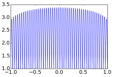
(a) The right hand side of Equation (3.2) in Klein as a function of $t\in{[}-1,1{]}$, which is claimed to be an upper bound on the Lebesgue function

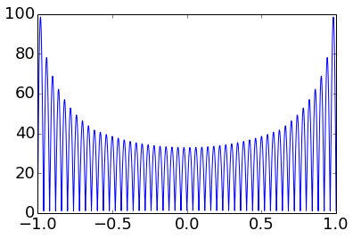
(b) The correct Lebesgue function

Figure 3: The correct Lebesgue function for $n=50$, $d=3$, $\tilde{n}=11$ and $\tilde{d}=7$.

The dependency of the Lebesgue function on the parameters $d$, $\tilde{n}$ and $\tilde{d}$ is subtle. For instance, Figure 4 shows that the Lebesgue function may decrease as we increase $d$ and keep the other parameters fixed. Moreover, the Lebesgue constant for $n=50$ and $d=\tilde{n}=\tilde{d}=7$ is $12$ times smaller than the Lebesgue constant if $n=50,$ $d=3$, $\tilde{n}=11$ and $\tilde{d}=7$, as considered in Klein .

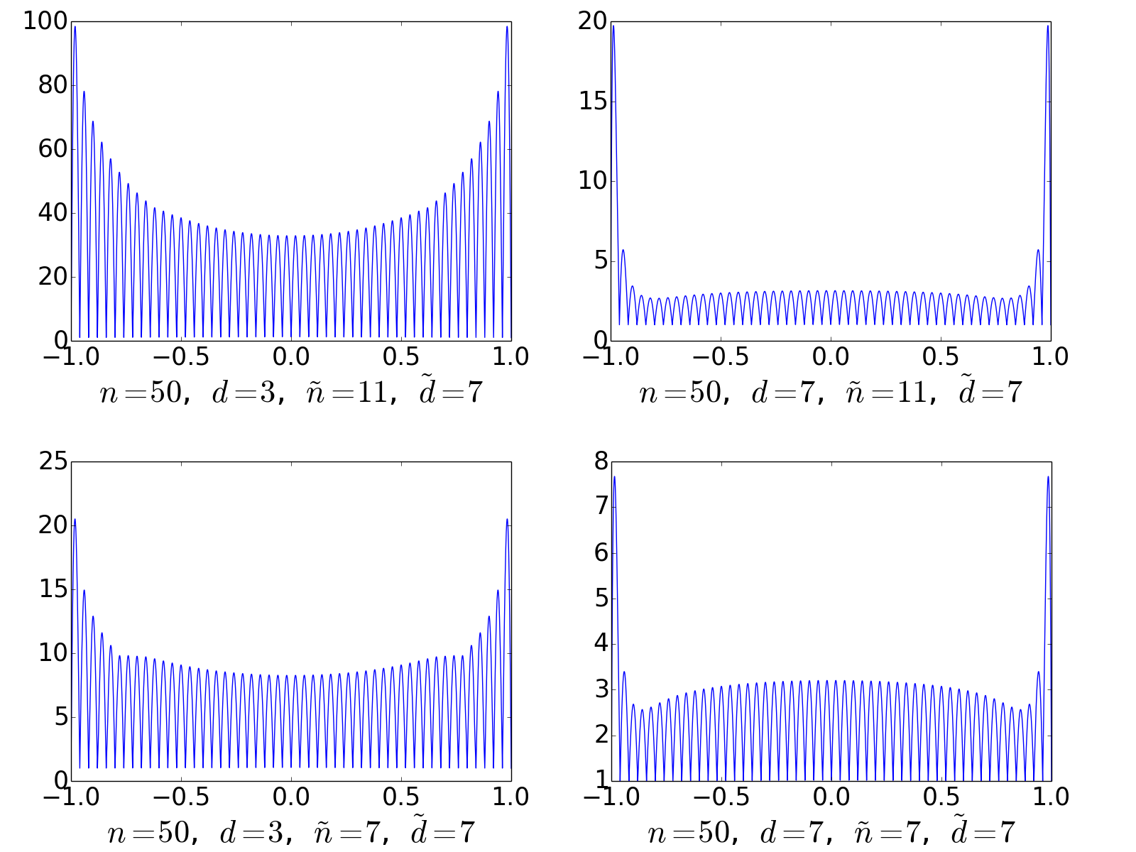
Figure 4: The dependency of the Lebesgue function on $d$, $\tilde{n}$ and $\tilde{d}$.

3.1 Proof of Lemma 1

In this subsection we prove Lemma 1 and show that when $n\leq 2\tilde{n}$ we have an analogous result with

$$\hskip 11.38092pt{c_{j}}\!\left(t\right) = \frac{\tilde{w}_{n,d,j}}{t-x_{j}}+\sum_{i=-d}^{-1}\frac{\tilde{w}_{n,d,i}\,a_{ij}}{t-\tilde{x}_{i}}\hskip 76.82234pt\mathrm{for}\ 0\leq j<n-\tilde{n},$$ (19)

$$\hskip 11.38092pt{c_{j}}\!\left(t\right) = \frac{\tilde{w}_{n,d,j}}{t-x_{j}}+\sum_{i=-d}^{-1}\frac{\tilde{w}_{n,d,i}\,a_{ij}}{t-\tilde{x}_{i}}$$

$$+ \sum_{i=n+1}^{n+d}\frac{\tilde{w}_{n,d,i}\,b_{\left(i-n\right)\left(j-n\right)}}{t-\tilde{x}_{i}}\hskip 73.97733pt\mathrm{for}\ n-\tilde{n}\leq j\leq\tilde{n},$$ (20)

$${c_{j}}\!\left(t\right) = \frac{\tilde{w}_{n,d,j}}{t-x_{j}}+\sum_{i=n+1}^{n+d}\frac{\tilde{w}_{n,d,i}\,b_{\left(i-n\right)\left(j-n\right)}}{t-\tilde{x}_{i}}\hskip 36.13512pt\mathrm{for}\ \tilde{n}<j\leq n.$$ (21)

Our proof involves the numbers $D^{(k)}_{ij}$ mentioned in the third section of KleinBerrutDerivatives , which represent the $k$th derivative at the node $x_{i}$ of the $j$th Lagrange fundamental rational function. In order to simplify the notation, we use the following lemma.

Lemma 2

Consider nodes $x_{0}<x_{1}<\dots<x_{\tilde{n}}$, weights $w_{0},w_{1},\dots,w_{\tilde{n}}\in\mathds{R}{}-{\left\{0\right\}}$, and the numbers $E^{(k)}_{ij}$, with $k\geq 0$ and $0\leq i,j\leq\tilde{n}$, defined inductively in $k$ by

$$E^{(0)}_{ii} := 1\hskip 28.45274pt\mathrm{and}\hskip 28.45274ptE^{(0)}_{ij}:=0\hskip 40.40285pt\mathrm{for}\ i\neq j.$$ (22)

$$E^{(k)}_{ij} := \frac{k}{x_{i}-x_{j}}\left(\frac{w_{j}}{w_{i}}E_{ii}^{\left(k-1\right)}-E_{ij}^{\left(k-1\right)}\right)\hskip 25.6073pt\mathrm{for}\ i\neq j,$$ (23)

$$E_{ii}^{(k)} := -\sum_{j=0,j\neq i}^{\tilde{n}}E_{ij}^{(k)}.$$ (24)

If $k>0$ then $E^{(k)}_{ij}$ is equal to the number $D^{(k)}_{ij}$ in Equations (3.1) and (3.2) in KleinBerrutDerivatives with $n$ replaced by $\tilde{n}$.

In order to prove this lemma, replace $k$ by $1$ in Equations (23) and (24), use (22) to simplify the result and Equation (3.2) of KleinBerrutDerivatives to verify that $E^{(1)}_{ij}=D^{(1)}_{ij}$. The case $k>1$ follows by induction from (23) and (24) and Equation (3.3) in KleinBerrutDerivatives .

Since we are assuming that the nodes are equally spaced, $x_{i}-x_{j}=\left(i-j\right)h$ and it is convenient to consider the normalized numbers

$$\overline{E}_{ij}^{(k)}:=h^{k}E_{ij}^{(k)}/k!.$$

Replacing $E_{ij}^{(k)}$ by $\overline{E}_{ij}^{(k)}k!\,h^{-k}$ in (22)–(24) we obtain

$$\hskip 11.38092pt\overline{E}^{(0)}_{ii} = 1\hskip 28.45274pt\mathrm{and}\hskip 28.45274pt\overline{E}^{(0)}_{ii}=0\hskip 49.22314pt\mathrm{for}\ i\neq j,$$ (25)

$$\hskip 11.38092pt\overline{E}^{(k)}_{ij} = \frac{1}{i-j}\left(\frac{w_{j}}{w_{i}}\overline{E}_{ii}^{\left(k-1\right)}-\overline{E}_{ij}^{\left(k-1\right)}\right)\hskip 41.82558pt\mathrm{for}\ i\neq j\hskip 5.69046pt\mathrm{and}\hskip 5.69046ptk\geq 1,$$ (26)

$$\hskip 11.38092pt\overline{E}_{ii}^{(k)} = -\sum_{j=0,j\neq i}^{\tilde{n}}\overline{E}_{ij}^{(k)}.$$ (27)

Equations (25)–(27) show that $\overline{E}^{(k)}_{ij}$ depends on $i$, $j$, $k$, and $\tilde{n}$, but it can depend on $h$, $d$, $n$ or $\tilde{d}$ only via the weights $w_{i}$, because there is no mention to $h$, $d$, $n$ and $\tilde{d}$ in (25) – (27). In the case that concerns us, the weights $w_{i}$ correspond to the usual Floater-Hormann interpolants in equally spaced nodes $x_{0},\dots,x_{\tilde{n}}$ with parameter $\delta=\tilde{d}$. These weights are given by (5), with $n$ and $\delta$ replaced by $\tilde{n}$ and $\tilde{d}$, and depend on $\tilde{n}$ and $\tilde{d}$, but not on $h$, $n$ or $d$. Therefore, in the case relevant to our discussion, $\overline{E}^{(k)}_{ij}$ does not depend on $h$, $n$ or $d$.

Equation (3.1) in KleinBerrutDerivatives and the identities $D_{ij}^{(k)}=E^{(k)}_{ij}$ for $k>0$ imply that

$${r^{(k)}_{\underline{\mathbf{x}},\tilde{d}}[\underline{\mathbf{y}}]}\!\left(x_{0}\right) = \sum_{j=0}^{\tilde{n}}D_{0j}^{(k)}y_{j}=\sum_{j=0}^{\tilde{n}}E_{0j}^{(k)}y_{j}=\frac{k!}{h^{k}}\sum_{j=0}^{\tilde{n}}\overline{E}_{0j}^{(k)}y_{j},$$

$${r^{(k)}_{\overline{\mathbf{x}},\tilde{d}}[\overline{\mathbf{y}}]}\!\left(x_{n}\right) = \sum_{j=n-\tilde{n}}^{n}D_{\tilde{n}\left(j-n+\tilde{n}\right)}^{(k)}y_{j}=\sum_{j=n-\tilde{n}}^{n}E_{\tilde{n}\left(j-n+\tilde{n}\right)}^{(k)}y_{j}=\frac{k!}{h^{k}}\sum_{j=n-\tilde{n}}^{n}\overline{E}_{\tilde{n}\left(j-n+\tilde{n}\right)}^{(k)}y_{j},$$

for $k>0$. Combining the last two equations with the identities $\overline{E}^{(0)}_{ii}=1$ and $\overline{E}^{(0)}_{ij}=0$ for $i\neq j$ we can rewrite (6) and (8) as

$$\tilde{y}_{i} = \sum_{k=0}^{\tilde{d}}\sum_{j=0}^{\tilde{n}}\overline{E}_{0j}^{(k)}i^{k}y_{j}\ \hskip 96.73918pt\mathrm{for}\ -d\leq i<0,$$

$$\tilde{y}_{i} = \sum_{k=0}^{\tilde{d}}\sum_{j=n-\tilde{n}}^{n}\overline{E}_{\tilde{n}\left(j-n+\tilde{n}\right)}^{(k)}\left(i-n\right)^{k}y_{j}\ \hskip 28.45274pt\mathrm{for}\ n<i\leq n+d.$$

These equations are equivalent to (10) and (11) with

$$\hskip 22.76228pta_{ij} := \sum_{k=0}^{\tilde{d}}\overline{E}_{0j}^{(k)}i^{k}\hskip 36.98866pt\mathrm{for}\ -d\leq i<0\hskip 8.5359pt\mathrm{and}\hskip 8.5359pt0\leq j\leq\tilde{n},$$ (28)

$$\hskip 22.76228ptb_{ij} := \sum_{k=0}^{\tilde{d}}\overline{E}_{\tilde{n}\left(j+\tilde{n}\right)}^{(k)}i^{k}\hskip 22.76228pt\mathrm{for}\ 0<i\leq d\hskip 8.5359pt\mathrm{and}\hskip 8.5359pt-\tilde{n}\leq j\leq 0.$$ (29)

Since $\overline{E}_{ij}^{(k)}$ does not depend on $h$, $d$ or $n$, and there is no mention to $h$, $d$ or $n$ in the right hand side of Equations (28) and (29), its is clear that $a_{ij}$ and $b_{ij}$ do not depend on $h$, $d$ or $n$, as claimed in Lemma 1. Equation (9) yields

$${\tilde{r}_{\mathbf{x},d,\tilde{n},\tilde{d}}[\mathbf{y}]}\!\left(t\right)=\frac{1}{{Q}\!\left(t\right)}\sum_{i=-d}^{n+d}\frac{\tilde{w}_{n,d,i}\,\tilde{y}_{i}}{t-\tilde{x}_{i}}\hskip 28.45274pt\mathrm{with}\hskip 28.45274pt{Q}\!\left(t\right)=\sum_{i=-d}^{n+d}\frac{\tilde{w}_{n,d,i}}{t-\tilde{x}_{i}}.$$

It follows that

$${Q}\!\left(t\right){\tilde{r}_{\mathbf{x},d,\tilde{n},\tilde{d}}[\mathbf{y}]}\!\left(t\right)=\sum_{i=-d}^{-1}\frac{\tilde{w}_{n,d,i}}{t-\tilde{x}_{i}}\sum_{j=0}^{\tilde{n}}\,a_{ij}\,y_{j}+\sum_{j=0}^{n}\frac{\tilde{w}_{n,d,j}\,y_{j}}{t-x_{j}}\ +$$

$$\sum_{i=n+1}^{n+d}\frac{\tilde{w}_{n,d,i}}{t-\tilde{x}_{i}}\sum_{j=n-\tilde{n}}^{n}\,b_{\left(i-n\right)\left(j-n\right)}\,y_{j}=$$

$$\sum_{j=0}^{\tilde{n}}\sum_{i=-d}^{-1}\frac{\tilde{w}_{n,d,i}\,a_{ij}\,y_{j}}{t-\tilde{x}_{i}}+\sum_{j=0}^{n}\frac{\tilde{w}_{n,d,j}\,y_{j}}{t-x_{j}}+\sum_{j=n-\tilde{n}}^{n}\sum_{i=n+1}^{n+d}\frac{\tilde{w}_{n,d,i}\,b_{\left(i-n\right)\left(j-n\right)}\,y_{j}}{t-\tilde{x}_{i}}.$$ (30)

We now have two cases: (i) $\tilde{n}<n-\tilde{n}$ and (ii) $\tilde{n}\geq n-\tilde{n}$. In the first case we can rewrite (30) as

$${Q}\!\left(t\right){\tilde{r}_{\mathbf{x},d,\tilde{n},\tilde{d}}[\mathbf{y}]}\!\left(t\right)=\sum_{j=0}^{\tilde{n}}\left(\frac{\tilde{w}_{n,d,j}}{t-x_{j}}+\sum_{i=-d}^{-1}\frac{\tilde{w}_{n,d,i}\,a_{ij}}{t-\tilde{x}_{i}}\right)y_{j}\ +$$

$$\sum_{j=\tilde{n}+1}^{n-\tilde{n}-1}\frac{\tilde{w}_{n,d,j}}{t-x_{j}}\,y_{j}+\sum_{j=n-\tilde{n}}^{n}\left(\frac{\tilde{w}_{n,d,j}}{t-x_{j}}+\sum_{i=n+1}^{n+d}\frac{\tilde{w}_{n,d,i}\,b_{\left(i-n\right)\left(j-n\right)}}{t-\tilde{x}_{i}}\right)y_{j},$$

and this proves (12)–(15). When $\tilde{n}\geq n-\tilde{n}$, we can rewrite (30) as

$${Q}\!\left(t\right){\tilde{r}_{\mathbf{x},d,\tilde{n},\tilde{d}}[\mathbf{y}]}\!\left(t\right)=\sum_{j=0}^{n-\tilde{n}-1}\left(\frac{\tilde{w}_{n,d,j}}{t-x_{j}}+\sum_{i=-d}^{-1}\frac{\tilde{w}_{n,d,i}\,a_{ij}}{t-\tilde{x}_{i}}\right)y_{j}\ +$$

$$\sum_{j=n-\tilde{n}}^{\tilde{n}}\left(\sum_{i=-d}^{-1}\frac{\tilde{w}_{n,d,i}\,a_{ij}}{t-\tilde{x}_{i}}+\frac{\tilde{w}_{n,d,j}}{t-x_{j}}+\sum_{i=n+1}^{n+d}\frac{\tilde{w}_{n,d,i}\,b_{\left(i-n\right)\left(j-n\right)}}{t-\tilde{x}_{i}}\right)y_{j}\ +$$

$$\sum_{j=\tilde{n}+1}^{n}\left(\frac{\tilde{w}_{n,d,j}}{t-x_{j}}+\sum_{i=n+1}^{n+d}\frac{\tilde{w}_{n,d,i}\,b_{\left(i-n\right)\left(j-n\right)}}{t-\tilde{x}_{i}}\right)y_{j}.$$

This proves (19)–(21) and we are done. ∎

4 The Lebesgue constant when $d=\tilde{n}=\tilde{d}$

This section presents a proof that the Lebesgue constant of extended interpolants mentioned in BerrutKleinCAM and Klein grows exponentially with $d=\tilde{n}=\tilde{d}$. This shows that the peculiar interpretation of the Lebesgue constant mentioned in Klein does not capture essential points regarding the stability of extended Floater Hormann interpolants in general, because Equation (3.2) in Klein does not take properly into account how changes on $\mathbf{y}$ affect $\tilde{\mathbf{y}}$.

The Lebesgue constant of the extended interpolant ${\tilde{r}_{\mathbf{x},d,\tilde{n},\tilde{d}}[\mathbf{y}]}\!\left(t\right)$ in (9) is

$$\tilde{\Lambda}_{\mathbf{x},d,\tilde{n},\tilde{d}}{}:=\max_{x_{0}\leq t\leq x_{n}}{\tilde{\Lambda}_{\mathbf{x},d,\tilde{n},\tilde{d}}}\!\left(t\right),$$

for the Lebesgue function ${\tilde{\Lambda}_{\mathbf{x},d,\tilde{n},\tilde{d}}}\!\left(t\right)$ in (17), and the Lebesgue constant for polynomial interpolation at $d+1$ equally spaced nodes is

$$\Lambda_{d}:=\sup_{0\leq t\leq d,\ \ \mathbf{y}\in{\mathds{R}}^{d+1}-{\left\{0\right\}}}\frac{\left|{p_{d,\mathbf{y}}}\!\left(t\right)\right|}{\left\|{\mathbf{y}}\right\|_{\infty}},$$

where $p_{d,\mathbf{y}}$ is the polynomial with degree less than $d+1$ such that ${p_{d,\mathbf{y}}}\!\left(i\right)=y_{i}$ for $i=0,\dots,d$. In this section we show that $\tilde{\Lambda}_{\mathbf{x},d,d,d}{}$ is not much smaller than $\Lambda_{d}$, by providing a lower bound for $\tilde{\Lambda}_{\mathbf{x},d,d,d}{}$ which approaches $\Lambda_{d}$ exponentially fast as $d$ increases. Formally, we have the following:

Theorem 4.1

If $n>d+1\geq 3$ then $\tilde{\Lambda}_{\mathbf{x},d,d,d}{}\geq\kappa_{d}\Lambda_{d}$, for

$$\kappa_{d}:=\left(1-\frac{d}{2^{d}-1}-2^{-d}\right).$$ (31)

We prove Theorem 4.1 at the end of this section. For now, let us explore its consequences and check them experimentally. As explained in Trefe , we have

$$\frac{2^{d-2}}{d^{2}}<\Lambda_{d}<\frac{2^{d+3}}{d}.$$

Therefore, $\Lambda_{d}$ grows exponentially with $d$ and Theorem 4.1 shows that the same applies to $\tilde{\Lambda}_{\mathbf{x},d,d,d}{}$. Moreover, Bos et. al. Bos show that the Lebesgue constant for the Floater-Hormann interpolant at $\mathbf{x}$ with parameter $\delta$ satisfies $\tilde{\Lambda}_{\mathbf{x},\delta}{}\leq 2^{\delta-1}\left(2+\log n\right)$. Theorem 4.1 shows that $\Lambda_{d}<1.5\tilde{\Lambda}_{\mathbf{x},d,d,d}{}$ for $d\geq 4$, and combining the two equations above for $d\geq 4$ we conclude that, when $\delta=d$,

$$\tilde{\Lambda}_{\mathbf{x},\delta}{}<2d^{2}\left(2+\log n\right)\Lambda_{d}<3d^{2}\left(2+\log n\right)\tilde{\Lambda}_{\mathbf{x},d,d,d}{},$$

and the ratio $\tilde{\Lambda}_{\mathbf{x},\delta}{}/\tilde{\Lambda}_{\mathbf{x},d,d,d}{}$ is definitely not as large as claimed in Klein . This observation is corroborated by Figure 5.

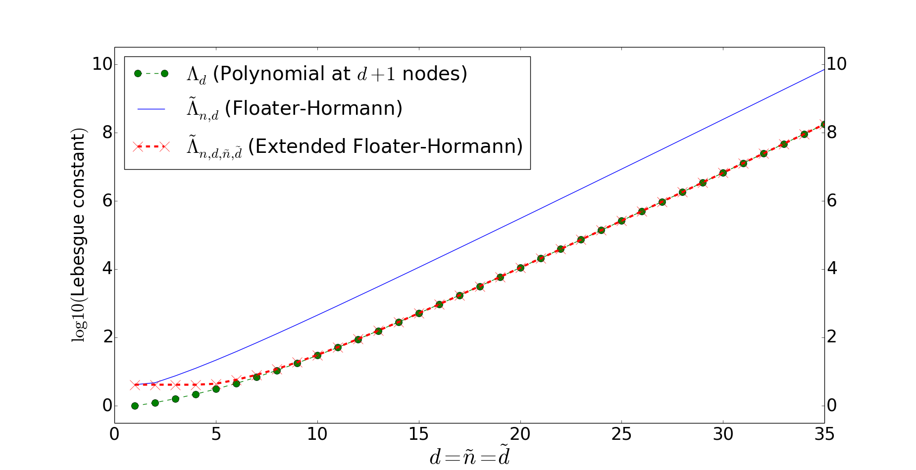
Figure 5: $\log\!{\rm 10}$ of the Lebesgue constants for $n=200$ and $\delta=d=\tilde{n}=\tilde{d}$ varying from $1$ to $35$. The Lebesgue constant of the extended interpolant is about the same as the Lebesgue constant for polynomial interpolation at $\left(d+1\right)$ equally spaced nodes for $d\geq 7$, and $\tilde{\Lambda}_{\mathbf{x},\delta}{}$ is roughly equal to $100\tilde{\Lambda}_{\mathbf{x},d,\tilde{n},\tilde{d}}{}$ for large $\delta=d=\tilde{n}=\tilde{d}$.

4.1 Proof of Theorem 4.1

We follow the usual convention that a sum of the form $\sum_{i=a}^{b}u_{i}$ with $b<a$ is equal to $0$ and a product $\prod_{i=a}^{b}u_{i}$ with $b<a$ is equal to $1$. According to Klein ,

$${\tilde{r}_{\mathbf{x},d,\tilde{n},\tilde{d}}[\mathbf{y}]}\!\left(t\right)=\frac{\sum\limits_{i=-d}^{n}\tilde{\lambda}_{i}(t,\tilde{\mathbf{x}})p_{i}(t,\tilde{\mathbf{x}},\mathbf{\tilde{y}})}{\sum\limits_{i=-d}^{n}\tilde{\lambda}_{i}(t,\tilde{\mathbf{x}})},$$ (32)

where $\tilde{x}_{i}=x_{0}+ih$ for $-d\leq i\leq n+d$, $\tilde{\mathbf{y}}=\left(\tilde{y}_{-d},\tilde{y}_{1-d},\,\dots\,,\tilde{y}_{n+d}\right)$ and

$${\tilde{\lambda}_{i}}\!\left(t,\tilde{\mathbf{x}}\right):=\frac{\left(-1\right)^{i}}{\left(t-\tilde{x}_{i}\right)\left(t-\tilde{x}_{i+1}\right)\dots\left(t-\tilde{x}_{i+d}\right)}\hskip 28.45274pt\mathrm{for}\ i=0,\dots,n,$$ (33)

and ${p_{i}}\!\left(t,\tilde{\mathbf{x}},\tilde{\mathbf{y}}\right)$ is the polynomial with degree less than $d+1$ such that ${p_{i}}\!\left(\tilde{x}_{k},\tilde{\mathbf{x}},\tilde{\mathbf{y}}\right)=\tilde{y}_{k}$ for $k=i,\dots,i+d$. When $\tilde{\mathbf{y}}$ is defined as in Equations (6)– (8), we have

$${p_{i}}\!\left(t,\tilde{\mathbf{x}},\mathbf{\tilde{y}}\right)={p_{i}}\!\left(t,\mathbf{x},\mathbf{y}\right)\ \ \ \mathrm{for}\ \ \ 0\leq i\leq n-d,$$

and when $d=\tilde{n}=\tilde{d}$ we also have

$${p_{i}}\!\left(t,\tilde{\mathbf{x}},\mathbf{\tilde{y}}\right) = {p_{0}}\!\left(t,\mathbf{x},\mathbf{y}\right)\hskip 39.83368pt\ \mathrm{for}\ -d\leq i<0,$$

$${p_{i}}\!\left(t,\tilde{\mathbf{x}},\mathbf{\tilde{y}}\right) = {p_{n-d}}\!\left(t,\mathbf{x},\mathbf{y}\right)\hskip 28.45274pt\ \mathrm{for}\ n-d<i\leq n,$$

because in this case the interpolants ${r_{\underline{\mathbf{x}},\tilde{d}}[\underline{\mathbf{y}}]}\!\left(t\right)$ and ${r_{\overline{\mathbf{x}},\tilde{d}}[\overline{\mathbf{y}}]\dot{}}\!\left(t\right)$ are polynomials, and the Taylor series of a polynomial is equal to itself. Equation (32) leads to

$${\tilde{r}_{\mathbf{x},d,d,d}[\mathbf{y}]}\!\left(t\right)=\frac{\left(\sum_{i=-d}^{0}{\tilde{\lambda}_{i}}\!\left(t,\tilde{\mathbf{x}}\right)\right){p_{0}}\!\left(t,\mathbf{x},\mathbf{y}\right)+{\tilde{\lambda}_{1}}\!\left(t,\mathbf{x}\right){p_{1}}\!\left(t,\mathbf{x},\mathbf{y}\right)}{\sum_{i=-d}^{n}{\tilde{\lambda}_{i}}\!\left(t,\tilde{\mathbf{x}}\right)}\ +$$

$$\frac{\sum_{i=2}^{n-d-1}{\tilde{\lambda}_{i}}\!\left(t,\mathbf{x}\right){p_{i}}\!\left(t,\mathbf{x},\mathbf{y}\right)}{\sum_{i=-d}^{n}{\tilde{\lambda}_{i}}\!\left(t,\tilde{\mathbf{x}}\right)}+\frac{\left(\sum_{i=n-d}^{n}\frac{{\tilde{\lambda}_{i}}\!\left(t,\tilde{\mathbf{x}}\right)}{{\tilde{\lambda}_{n-d}}\!\left(t,\mathbf{x}\right)}\right){\tilde{\lambda}_{n-d}}\!\left(t,\mathbf{x}\right){p_{n-d}}\!\left(t,\mathbf{x},\mathbf{y}\right)}{\sum_{i=-d}^{n}{\tilde{\lambda}_{i}}\!\left(t,\tilde{\mathbf{x}}\right)}.$$ (34)

(Since $n>d+1$ the sums in numerator of the first and last parcels in the expression above do not overlap, even when the sum in the numerator in the middle is empty.) Let $t\ \in\ (x_{0},x_{1})$ be fixed. We claim that $y^{*}_{0},y^{*}_{1},\dots,y^{*}_{n}\ \in\ \{-1,1\}$ defined by

$$y^{*}_{0}:=y^{*}_{1}:=(-1)^{d}\hskip 17.07182pt\mathrm{and}\hskip 17.07182pty^{*}_{j}:=(-1)^{d+j-1}\ \mathrm{for}\ \ 2\leq j\leq n$$

satisfy

$${\tilde{\lambda}_{i}}\!\left(t,\mathbf{x}\right){p_{i}}\!\left(t,\mathbf{x},\mathbf{y^{*}}\right)=\sum\limits_{j=0}^{d}\frac{\left|u_{j}\right|}{\left|t-\tilde{x}_{i+j}\right|}\geq 0\hskip 11.38092pt\mathrm{for}\ i=0\ \mbox{or}\ 2\leq i\leq n-d,$$ (35)

where

$$u_{j}:=\frac{(-1)^{d-j}}{d!h^{d}}\left(\begin{array}[]{c}d\\ j\end{array}\right).$$

In fact, (33) and Equations (3.1), (3.3) and (5.1) of Ber show that

$$\tilde{\lambda}_{i}(t,\mathbf{x})p_{i}(t,\mathbf{x},\mathbf{y^{*}})=(-1)^{i}\sum\limits_{j=0}^{d}\frac{u_{j}y^{*}_{i+j}}{t-x_{i+j}},$$ (36)

and (35) follows from

$$\frac{u_{0}y^{*}_{0}}{t-x_{0}}=\frac{\left|u_{0}\right|}{\left|t-x_{0}\right|},\hskip 28.45274pt\frac{u_{1}y^{*}_{1}}{t-x_{1}}=\frac{\left|u_{1}\right|}{\left|t-x_{1}\right|}$$

and

$$\frac{u_{j}y^{*}_{i+j}}{t-x_{i+j}}=\frac{(-1)^{d-j}\left|u_{j}\right|y^{*}_{i+j}}{t-x_{i+j}}=\frac{(-1)^{i-1}\left|u_{j}\right|}{t-x_{i+j}}=\frac{(-1)^{i}\left|u_{j}\right|}{\left|t-x_{i+j}\right|}$$

for $2\leq i+j\leq n$ and $0\leq j\leq d$.

Note that

$$\frac{\sum_{i=-d}^{0}{\tilde{\lambda}_{i}}\!\left(t,\tilde{\mathbf{x}}\right)}{\tilde{\lambda}_{0}(t,\mathbf{x})}>0,$$ (37)

because, for $-d\leq i<0$, we have that $d+i+1\geq 1$ and (33) yields

$$\frac{{\tilde{\lambda}_{i}}\!\left(t,\tilde{\mathbf{x}}\right)}{{\tilde{\lambda}_{0}}\!\left(t,\tilde{\mathbf{x}}\right)}=\frac{\left(-1\right)^{i}\left(t-x_{0}\right)\dots\left(t-x_{d+i}\right)\left(t-x_{d+i+1}\right)\dots\left(t-x_{d}\right)}{\left(t-\tilde{x}_{i}\right)\dots\left(t-\tilde{x}_{-1}\right)\left(t-x_{0}\right)\dots\left(t-x_{d+i}\right)}$$

$$=\frac{\left(-1\right)^{i}\left(t-x_{d+i+1}\right)\dots\left(t-x_{d}\right)}{\left|t-\tilde{x}_{i}\right|\dots\left|t-\tilde{x}_{-1}\right|}=\frac{\left|t-x_{d+i+1}\right|\dots\left|t-x_{d}\right|}{\left|t-\tilde{x}_{i}\right|\dots\left|t-\tilde{x}_{-1}\right|}\geq 0,$$ (38)

and this inequality also holds for $i=0$. Moreover, the signs of the numbers $\tilde{\lambda}_{1}(t,\tilde{\mathbf{x}})$, $\tilde{\lambda}_{2}(t,\tilde{\mathbf{x}})$, $\dots$, $\tilde{\lambda}_{n}(t,\tilde{\mathbf{x}})$ alternate, and their magnitude decreases because, for $1\leq i<n$, (33) yields

$$-1<\frac{\tilde{\lambda}_{i+1}(t,\tilde{\mathbf{x}})}{\tilde{\lambda}_{i}(t,\tilde{\mathbf{x}})}=-\frac{\tilde{x}_{i}-t}{\tilde{x}_{d+i+1}-t}<0.$$ (39)

As a result,

$$\sum_{i=n-d}^{n}\frac{{\tilde{\lambda}_{i}}\!\left(t,\tilde{\mathbf{x}}\right)}{{\tilde{\lambda}_{n-d}}\!\left(t,\mathbf{x}\right)}\geq 0.$$

This inequality and (35) with $i=n-d$ imply that the numerator of the last parcel in the sum in the right hand side of (34) is not negative, and combining (34), (35) and (37) we obtain

$$\left|{\tilde{r}_{\mathbf{x},d,d,d}[\mathbf{y}^{*}]}\!\left(t\right)\right|\geq\frac{\frac{\sum_{i=-d}^{0}\tilde{\lambda}_{i}(t,\tilde{\mathbf{x}})}{\vspace{0.5mm}\tilde{\lambda}_{0}(t,\mathbf{x})}\tilde{\lambda}_{0}(t,\mathbf{x})p_{0}(t,\mathbf{x},\mathbf{y^{*}})-\left|\tilde{\lambda}_{1}(t,\mathbf{x})p_{1}(t,\mathbf{x},\mathbf{y^{*}})\right|}{\left|\sum_{i=-d}^{n}\tilde{\lambda}_{i}(t,\tilde{\mathbf{x}})\right|}.$$ (40)

Moreover, (35) and (36) yield

$$\tilde{\lambda}_{0}(t,\mathbf{x})p_{0}(t,\mathbf{x},\mathbf{y^{*}})-\left|\tilde{\lambda}_{1}(t,\mathbf{x})p_{1}(t,\mathbf{x},\mathbf{y^{*}})\right|\ \ \geq\ \ \sum\limits_{j=0}^{d}\frac{\left|u_{j}\right|}{\left|t-x_{j}\right|}-\sum\limits_{j=0}^{d}\frac{\left|u_{j}\right|}{\left|t-x_{j+1}\right|}$$

$$\geq\ \frac{\left|u_{0}\right|}{\left|t-x_{0}\right|}+{\left\{\frac{\left|u_{1}\right|-\left|u_{0}\right|}{\left|t-x_{1}\right|}-\frac{\left|u_{1}\right|}{\left|t-x_{2}\right|}\right\}}+\sum\limits_{j=2}^{d}\left(\frac{\left|u_{j}\right|}{\left|t-x_{j}\right|}-\frac{\left|u_{j}\right|}{\left|t-x_{j+1}\right|}\right).$$ (41)

The last sum in (41) is positive for all $t\ \in\ (x_{0},x_{1})$. The term in brackets is also positive for $t\ \in\ (x_{0},x_{1})$, because

$$\frac{\left|u_{1}\right|-\left|u_{0}\right|}{\left|u_{1}\right|}=1-\frac{1}{d}\geq\frac{1}{2}\geq\frac{\left|t-x_{1}\right|}{\left|t-x_{2}\right|}.$$

Therefore,

$$\tilde{\lambda}_{0}(t,\mathbf{x})p_{0}(t,\mathbf{x},\mathbf{y^{*}})-\left|\tilde{\lambda}_{1}(t,\mathbf{x})p_{1}(t,\mathbf{x},\mathbf{y^{*}})\right|\ \ \geq\ \ 0.$$ (42)

Equation (38) shows that the numbers $\tilde{\lambda}_{-d}(t,\tilde{\mathbf{x}})$, $\tilde{\lambda}_{1-d}(t,\tilde{\mathbf{x}})$, $\dots$, $\tilde{\lambda}_{-1}(t,\tilde{\mathbf{x}})$ have the same sign as $\tilde{\lambda}_{0}(t,\tilde{\mathbf{x}})$. When $-d<i\leq 0$ we also have

$$\frac{\tilde{\lambda}_{i}(t,\tilde{\mathbf{x}})}{\tilde{\lambda}_{1}(t,\tilde{\mathbf{x}})}=\frac{\left(-1\right)^{i+1}\left(t-x_{1}\right)\dots\left(t-x_{d+i}\right)\left(t-x_{d+i+1}\right)\dots\left(t-x_{d+1}\right)}{\left(t-\tilde{x}_{i}\right)\dots\left(t-x_{0}\right)\left(t-x_{1}\right)\dots\left(t-x_{d+i}\right)}=$$

$$\frac{\left(-1\right)^{i+1}\left(t-x_{d+i+1}\right)\dots\left(t-x_{d+1}\right)}{\left(t-\tilde{x}_{i}\right)\dots\left(t-x_{0}\right)}=\frac{\left(x_{d+i+1}-t\right)\dots\left(x_{d+1}-t\right)}{\left(t-\tilde{x}_{i}\right)\dots\left(t-x_{0}\right)}\geq 0,$$ (43)

and the reader can verify that this inequality also holds for $i=-d$. Therefore,

$$\frac{\tilde{\lambda}_{i}(t,\tilde{\mathbf{x}})}{\tilde{\lambda}_{1}(t,\tilde{\mathbf{x}})}>0\hskip 28.45274pt\mathrm{for}\hskip 5.69046pt-d\leq i\leq 1.$$ (44)

Since all ${\tilde{\lambda}_{i}}\!\left(t,\mathbf{x}\right)$ for $-d\leq 0\leq 1$ have the same sign, and for $i\geq 1$ the signs of the ${\tilde{\lambda}_{i}}\!\left(t,\mathbf{x}\right)$ alternate and their magnitude decreases, we have

$$\left|\sum_{i=-d}^{n}{\tilde{\lambda}_{i}}\!\left(t,\tilde{\mathbf{x}}\right)\right|\leq\left|\sum_{i=-d}^{1}{\tilde{\lambda}_{i}}\!\left(t,\tilde{\mathbf{x}}\right)\right|.$$ (45)

Equations (40), (42) and (45) lead to

$$\left|{\tilde{r}_{\mathbf{x},d,d,d}[\mathbf{y}^{*}]}\!\left(t\right)\right|\geq\frac{\left|\sum_{i=-d}^{-1}\tilde{\lambda}_{i}(t,\tilde{\mathbf{x}})\right|\left|p_{0}(t,\mathbf{x},\mathbf{y^{*}})\right|}{\left|\sum_{i=-d}^{1}\tilde{\lambda}_{i}(t,\tilde{\mathbf{x}})\right|}.$$ (46)

When $-d<i\leq 0$, Equation (38), and the comment just after it, yield

$$\frac{{\tilde{\lambda}_{i}}\!\left(t,\tilde{\mathbf{x}}\right)}{{\tilde{\lambda}_{0}}\!\left(t,\tilde{\mathbf{x}}\right)}\geq\frac{\left(x_{d+i+1}-x_{1}\right)\dots\left(x_{d}-x_{1}\right)}{\left(x_{1}-\tilde{x}_{i}\right)\dots\left(x_{1}-\tilde{x}_{-1}\right)}=\frac{\left(d+i\right)\dots\left(d-1\right)h^{-i}}{\left(1-i\right)!h^{-i}}=$$

$$\frac{\left(d+i\right)\dots\left(d-1\right)}{\left(1-i\right)!}=\frac{1}{d}{\left(\begin{array}[]{c}d\\ 1-i\end{array}\right)}.$$

Therefore,

$$d\times\frac{\sum_{i=-d}^{1}\left|{\tilde{\lambda}_{i}}\!\left(t,\tilde{\mathbf{x}}\right)\right|}{\left|{\tilde{\lambda}_{0}}\!\left(t,\tilde{\mathbf{x}}\right)\right|}\geq\sum_{i=1-d}^{0}{\left(\begin{array}[]{c}d\\ 1-i\end{array}\right)}=\sum_{j=1}^{d}{\left(\begin{array}[]{c}d\\ j\end{array}\right)}=2^{d}-1.$$ (47)

Moreover, for $-d<i\leq 0$ Equation (43) yields

$$\frac{\tilde{\lambda}_{i}(t,\tilde{\mathbf{x}})}{\tilde{\lambda}_{1}(t,\tilde{\mathbf{x}})}\geq\frac{\left(x_{d+i+1}-x_{1}\right)\dots\left(x_{d+1}-x_{1}\right)}{\left(x_{1}-\tilde{x}_{i}\right)\dots\left(x_{1}-x_{0}\right)}=\frac{\left(d+i\right)\dots d\,h^{1-i}}{\left(1-i\right)!h^{1-i}}={\left(\begin{array}[]{c}d\\ 1-i\end{array}\right)},$$

and

$$\frac{\sum_{i=-d}^{1}\left|\tilde{\lambda}_{i}(t,\tilde{\mathbf{x}})\right|}{\left|\tilde{\lambda}_{1}(t,\tilde{\mathbf{x}})\right|}\geq\sum_{i=1-d}^{0}\frac{\left|\tilde{\lambda}_{i}(t,\tilde{\mathbf{x}})\right|}{\left|\tilde{\lambda}_{1}(t,\tilde{\mathbf{x}})\right|}+1\geq\sum_{i=1-d}^{1}{\left(\begin{array}[]{c}d\\ 1-i\end{array}\right)}=\sum_{j=0}^{d}{\left(\begin{array}[]{c}d\\ j\end{array}\right)}=2^{d}.$$ (48)

It follows from Equations (31), (47) and (48) that

$$\left|\sum_{i=-d}^{-1}\tilde{\lambda}_{i}(t,\tilde{\mathbf{x}})\right|=\sum_{i=-d}^{-1}\left|\tilde{\lambda}_{i}(t,\tilde{\mathbf{x}})\right|=\sum_{i=-d}^{1}\left|\tilde{\lambda}_{i}(t,\tilde{\mathbf{x}})\right|-\left|\tilde{\lambda}_{0}(t,\tilde{\mathbf{x}})\right|-\left|\tilde{\lambda}_{1}(t,\tilde{\mathbf{x}})\right|$$

$$=\left(1-\frac{\left|\tilde{\lambda}_{0}(t,\tilde{\mathbf{x}})\right|}{\sum_{i=-d}^{1}\left|\tilde{\lambda}_{i}(t,\tilde{\mathbf{x}})\right|}-\frac{\left|\tilde{\lambda}_{1}(t,\tilde{\mathbf{x}})\right|}{\sum_{i=-d}^{1}\left|\tilde{\lambda}_{i}(t,\tilde{\mathbf{x}})\right|}\right)\sum_{i=-d}^{1}\left|\tilde{\lambda}_{i}(t,\tilde{\mathbf{x}})\right|\geq\kappa_{d}\left|\sum_{i=-d}^{1}\tilde{\lambda}_{i}(t,\tilde{\mathbf{x}})\right|.$$

The inequality in the previous line and (46) yield

$$\left|{\tilde{r}_{\mathbf{x},d,d,d}[\mathbf{y}^{*}]}\!\left(t\right)\right|\geq\kappa_{d}\left|p_{0}(t,\mathbf{x},\mathbf{y^{*}})\right|.$$

Equation (35) shows that, for $t\ \in[x_{0},x_{1}]$, $\left|p_{0}(.,\mathbf{x},\mathbf{y^{*}})\right|$ is identical to the Lebesgue function for polynomial interpolation at $(d+1)$ equally spaced nodes in $[x_{0},x_{d}]$. According to Brutman , the Lebesgue function for polynomial interpolation at equally spaced nodes attains its maximum at some $t^{*}\in(x_{0},x_{1})$. For this $t^{*}$ we have

$$\tilde{\Lambda}_{\mathbf{x},d,d,d}{}\geq{\tilde{\Lambda}_{\mathbf{x},d,d,d}}\!\left(t^{*}\right)\ \geq\ \left|{\tilde{r}_{\mathbf{x},d,d,d}[\mathbf{y^{*}}]}\!\left(t^{*}\right)\right|\ \geq\kappa_{d}\left|{p_{0}}\!\left(t^{*},\mathbf{x},\mathbf{y^{*}}\right)\right|=\kappa_{d}\Lambda_{d},$$

and this completes the proof of Theorem 4.1. ∎

5 Backward instability

In this section we discuss the backward stability of the barycentric formula used to evaluate extended interpolants when $\tilde{\mathbf{y}}$ is given by a function ${Y}\!\left(d,\mathbf{x},\mathbf{y}\right)$ which is linear in $\mathbf{y}$. Formally, we take $\tilde{y}_{i}:=y_{i}$ for $0\leq i\leq n$ and

$$\tilde{y}_{i}:={Y_{i}}\!\left(d,\mathbf{x},\mathbf{y}\right)=\sum_{j=0}^{n}{h_{ij}}\!\left(d,\mathbf{x}\right)y_{j}\hskip 28.45274pt\mathrm{for}\hskip 5.69046pti\in{\left\{-d,\dots,n+d\right\}}\setminus{\left\{0,\dots,n\right\}}.$$ (49)

The extended function values $\tilde{\mathbf{y}}$ are supposed to be evaluated numerically and then to be used to evaluate the barycentric interpolant ${b}\!\left(t,\mathbf{y}\right)$ given by

$${b}\!\left(t,\mathbf{y}\right):=\left.\sum_{i=-d}^{n+d}\frac{\tilde{w}_{i}\tilde{y}_{i}}{t-\tilde{x}_{i}}\right/\sum_{i=-d}^{n+d}\frac{\tilde{w}_{i}}{t-\tilde{x}_{i}}\hskip 14.22636pt\mathrm{with}\hskip 14.22636pt\tilde{y}_{i}={Y_{i}}\!\left(d,\mathbf{x},\mathbf{y}\right).$$ (50)

We assume that the weights $\tilde{w}_{i}$ are such that the denominator of ${b}\!\left(t,\mathbf{y}\right)$ is different from zero for $t\in[x_{0},x_{n}]\setminus{\left\{x_{0},x_{1},\dots x_{n}\right\}}$.

As we have shown in Section 3, the Equation (2.3) in Klein and the equation just before Theorem 5.1 in BerrutKleinCAM are particular cases of Equation (50). Therefore, by discussing the backward stability of (49)–(50) we also cover the the backward stability of the interpolation formulae proposed in the literature.

In order to analyze the backward stability of (49)–(50), it is convenient to proceed as in Section 3 and rewrite (50) as

$${b}\!\left(t,\mathbf{y}\right)=\left.\sum_{i=0}^{n}{d_{i}}\!\left(t\right)y_{i}\right/\sum_{i=-d}^{n+d}\frac{\tilde{w}_{i}}{t-\tilde{x}_{i}},$$ (51)

for

$${d_{j}}\!\left(t\right):=\sum_{i=-d}^{-1}\frac{\tilde{w}_{i}{h_{ij}}\!\left(d,\mathbf{x}\right)}{t-\tilde{x}_{i}}+\frac{\tilde{w}_{j}}{t-x_{j}}+\sum_{i=n+1}^{n+d}\frac{\tilde{w}_{i}{h_{ij}}\!\left(d,\mathbf{x}\right)}{t-\tilde{x}_{i}}.$$ (52)

Equations (51)–(52) can be verified as in the proof of the validity of the reduced form (12) presented in Section 3.1.

We adopt the definition of backward stability used by Higham in HIGHAM_IMA , that is, the formulae above are backward stable when the value ${\hat{b}}\!\left(t,\mathbf{y}\right)$ obtained by evaluating (49)-(50) in inexact arithmetic is equal to the exact value ${b}\!\left(t,\hat{\mathbf{y}}\right)$ for a perturbed vector $\hat{\mathbf{y}}$ with $\hat{y}_{i}=y_{i}\left(1+\phi_{i}\right)$ for $\phi_{i}$ small. With this in mind, we can summarize this section as follows:

The barycentric formula (49)-(50) is not backward stable in Higham’s sense when $\tilde{w}_{k}\neq 0$ for some $k\in{\left\{-d,\dots,n+d\right\}}\setminus{\left\{0,\dots n\right\}}$ and there exists $t\in[x_{0},x_{n}]\setminus{\left\{x_{0},x_{1},\dots x_{n}\right\}}$ and $0\leq j\leq n$ such that ${d_{j}}\!\left(t\right)=0$.

In this circumstance, we can prove the backward instability of (49)-(50) by considering $\mathbf{y}\in{\mathds{R}}^{n+1}$ with $y_{j}=1$ and $y_{i}=0$ for $i\neq j$ and all $\hat{\mathbf{y}}\in{\mathds{R}}^{n+1}$ with $\hat{y}_{i}=y_{i}\left(1+\phi_{i}\right)$ for some $\phi_{i}\in\mathds{R}{}$. On the one hand, we have that ${d_{i}}\!\left(t\right)y_{i}\left(1+\phi_{i}\right)=0$ for all $i$ and $\phi_{i}\in\mathds{R}{}$, because ${d_{j}}\!\left(t\right)=0$ and $y_{i}=0$ for $i\neq j$. Therefore, Equation (51) shows that when we evaluate (49)-(50) in exact arithmetic with $t$ and $\hat{\mathbf{y}}$ we obtain ${b}\!\left(t,\hat{\mathbf{y}}\right)=0$. On the other hand, if the unique rounding error occurs in the evaluation of Equation (49) for $i=k$, so that $\tilde{y}_{k}$ is computed as $\tilde{y}_{k}+\xi$ for $\xi\neq 0$, then equation (51) shows that the computed value ${\hat{b}}\!\left(t,\mathbf{y}\right)$ satisfies

$${\hat{b}}\!\left(t,\mathbf{y}\right)=\left.\left(\frac{\tilde{w}_{k}\xi}{t-\tilde{x}_{k}}+\sum_{i=-d}^{n+d}\frac{\tilde{w}_{i}\tilde{y}_{i}}{t-\tilde{x}_{i}}\right)\right/\sum_{i=-d}^{n+d}\frac{\tilde{w}_{i}}{t-\tilde{x}_{i}}$$

$$=\left.\frac{\tilde{w}_{k}\xi}{t-\tilde{x}_{k}}\right/\sum_{i=-d}^{n+d}\frac{\tilde{w}_{i}}{t-\tilde{x}_{i}}+{b}\!\left(t,\mathbf{y}\right)=\left.\frac{\tilde{w}_{k}\xi}{t-\tilde{x}_{k}}\right/\sum_{i=-d}^{n+d}\frac{\tilde{w}_{i}}{t-\tilde{x}_{i}}\neq 0={b}\!\left(t,\hat{\mathbf{y}}\right).$$

Therefore, the computed value ${\hat{b}}\!\left(t,\mathbf{y}\right)$ differs from all the exact values ${b}\!\left(t,\hat{\mathbf{y}}\right)$ and, according to Higham’s definition, (49)-(50) is not backward stable in this case.

In practice the $\tilde{w}_{k}$ are different from zero and the simple condition ${d_{j}}\!\left(t\right)=0$ implies the backward instability of (49)-(50). We conclude this section with Figure 6, which shows that there is $t\in[x_{0},x_{n}]\setminus{\left\{x_{0},\dots,x_{n}\right\}}$ for which ${d_{2}}\!\left(t\right)=0$ for the extended interpolant with $n=50$, $d=3$, $\tilde{n}=11$ and $\tilde{d}=7$ considered by Klein . In fact, in this case $h=2/50=0.04$, $x_{2}=-0.92$, $x_{3}=-0.88$ and the function ${d_{2}}\!\left(t\right)$ has a zero in the interval $[-0.918,-0.914]\subset(x_{2},x_{3})$.

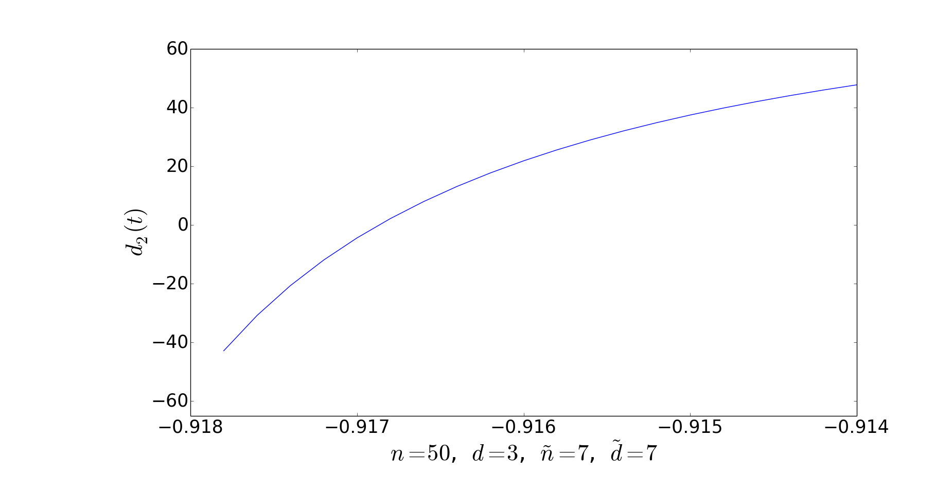
Figure 6: The function ${d_{2}}\!\left(t\right)$ for the extended interpolant with $n=50$, $d=3$, $\tilde{n}=11$ and $\tilde{d}=7$ considered in Klein .

6 Sources of numerical instability for extended interpolants

This section shows that extended interpolants based on extrapolation are strongly affected by the numerical errors in the extrapolation step when $\tilde{d}$ is large. The current literature pays little attention to this point and presents experimental comparisons of usual and extended interpolants that highlight cases in which $\tilde{d}$ is much smaller than $d$. Such experiments are biased in favor of extended interpolants: increasing $\delta$ for usual interpolants makes as much sense as increasing $\tilde{d}$ for extended interpolants when $d>\tilde{d}$, because for $d>\tilde{d}$ the order of approximation of the extended interpolants is $h^{\tilde{d}+1}$, and not $h^{d+1}$.

We consider the case $\delta=d=\tilde{d}=\tilde{n}$. In our judgment, this is the most relevant case because it is the minimal one resulting in the same approximation of order $h^{d+1}$ for extended interpolants and usual interpolants. This point is reinforced by Figure 7, which shows that it is pointless to increase $d$ when $d>\tilde{d}$.

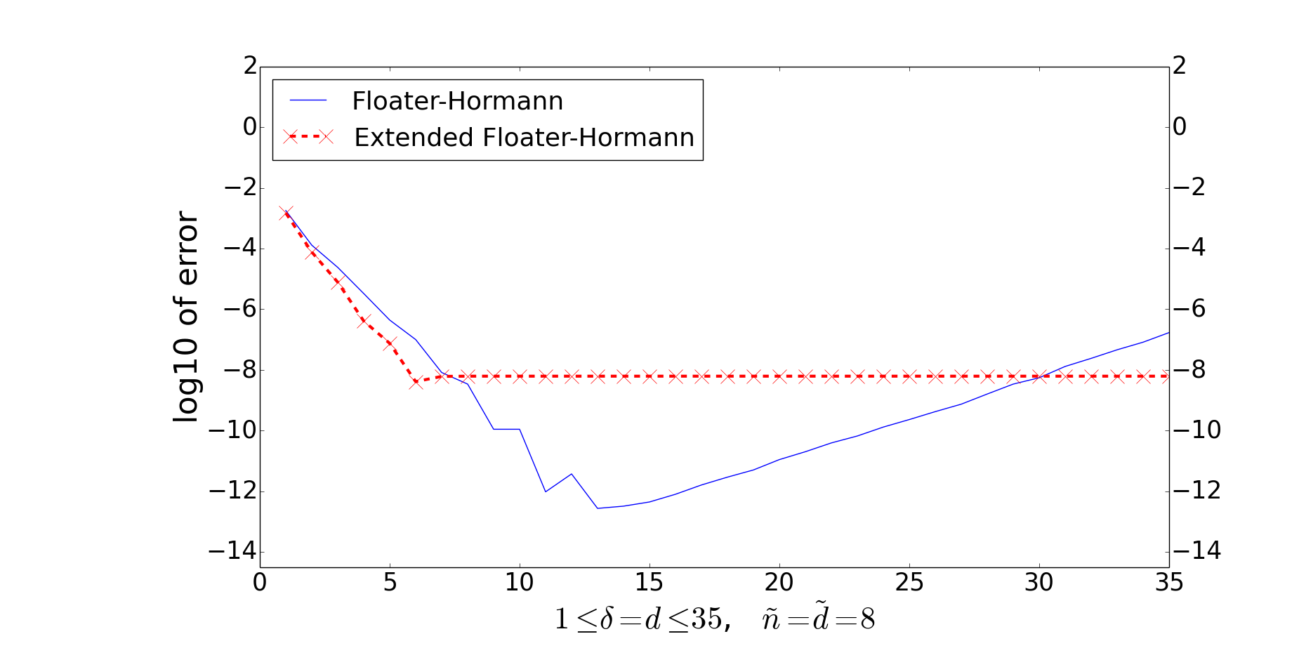
Figure 7: Log10 of the error for ${f}\!\left(t\right)={\sin}\!\left(20t\right)$ and $t\in[-1,1]$, with $n=200$, $\tilde{n}=\tilde{d}=8$ and $\delta=d$ varying from $1$ to $35$. Note that by simply increasing $d$, with an inappropriate $\tilde{d}$, we may obtain inaccurate results for extended interpolants. In this example, increasing $d$ when $d>\tilde{d}=8$ has no effect on the accuracy of the extended interpolant, but increasing $\delta$ up to $13$ improves the accuracy of the usual interpolants. This shows that the roles of $d$ and $\delta$ are quite different when $d>\tilde{d}$.

Figure 7 illustrates the importance of choosing appropriate $\tilde{d}$ for extended interpolants and makes clear the distinction between $d$ and $\delta$. Large values of $\delta$ have a devastating effect on usual Floater-Hormann interpolants, and this basic fact is mentioned explicitly in the documentation of libraries that implement these interpolants ALGLIB . Consequently, there is little to be learned from comparisons of extended and usual Floater-Hormann interpolants as in Figures 6 of BerrutKleinCAM and Klein : they fix $\tilde{d}$ at small values for extended interpolants and then raise $d=\delta$ to values as large as 50. Such choices of a large $d=\delta$ have no practical motivation for extended interpolants and are unfavorable to usual Floater-Hormann interpolants.

From this point to the end of this section we consider the interpolation of ${f}\!\left(t\right)={\sin}\!\left(20t\right)$ for $t\in[-1,1]$ with $n=200$. Figure 8 compares usual Floater-Hormann interpolants, extended interpolants with $\tilde{\mathbf{y}}$ computed in double precision and extended interpolants with precise $\tilde{\mathbf{y}}$. By precise we mean that $\tilde{\mathbf{y}}$ was computed using the MPFR library MPFR , with floating point numbers with a mantissa of 320 bits, from $\mathbf{y}$ computed with the same high precision.

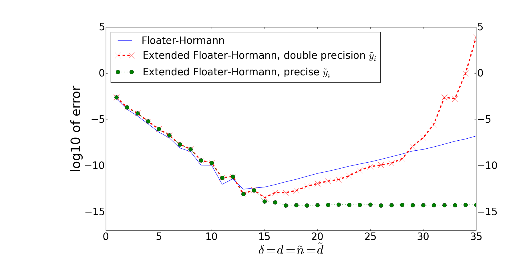
Figure 8: Log10 of the error for ${f}\!\left(t\right)={\sin}\!\left(20t\right)$, $t\in[-1,1]$ and $n=200$.

By error in our plots we mean the maximum difference between the numerically evaluated interpolant and the original function at $10^{7}$ equally spaced points in $[-1,1]$. The barycentric formula (4) and (9) were evaluated in double precision ($\epsilon\approx 10^{-16}$), using straightforward C++ code. The $\mathbf{y}$ and $\tilde{\mathbf{y}}$ computed in multiple precision were rounded to double precision and the barycentric formula corresponding to them was also evaluated in double precision. In other words, the case precise $\tilde{\mathbf{y}}$ differs from the other cases only by the precision of the $\tilde{\mathbf{y}}$, and not by the precision used to evaluate the barycentric formulae (4) and (9).

Figure 8 shows that, when the $\tilde{y}_{i}$ are evaluated in double precision, extended interpolants are not significantly more accurate than usual ones with $\delta=d$, and they become more unstable as $d=\tilde{d}=\tilde{n}$ grows. By contrast, extended interpolants with precise $\tilde{\mathbf{y}}$ are remarkably accurate, even for large values of $d=\tilde{d}=\tilde{n}$. This suggests that the inaccuracy of $\tilde{\mathbf{y}}$ is the cause of the numerical instability of extended interpolants for large $d=\tilde{d}=\tilde{n}$.

Figure 9 considers the ratio “error divided by Lebesgue constant.” This ratio is relevant for the understanding of the backward stability of interpolation formulae. As we explain in Andre , it is possible to implement the usual Floater-Hormann interpolants so that the backward error is of order $n\epsilon$. Backward errors of this order lead to forward errors of order $n\epsilon\Lambda_{\mathbf{x},\delta}\left\|{\mathbf{y}}\right\|_{\infty}$, as one can verify by looking at Figures 9 and 12 (in this article we refer to the forward error simply as error.) Therefore, in this case by dividing the error by the Lebesgue constant we obtain an estimate of the backward error. Unfortunately, Figure 9 shows that the relation between rounding errors and the Lebesgue constant for large values of $d=\tilde{d}=\tilde{n}$ for extended interpolant is more complex than the analogous relation for usual Floater-Hormann interpolants with $\delta=d$. As a result, the fact that extended interpolants have a smaller Lebesgue constant does not imply that they are more stable for large values of $\delta=d=\tilde{d}=\tilde{n}$ (see Figure 5.) In fact, in this scenario the effects of the large Lebesgue constants are quite different for extended and usual Floater-Hormann interpolants.

The combination of Figures 5 and 8 leads to a surprising observation: according to Figure 5, the Lebesgue constant of the usual interpolants in our experiments is about $100$ times larger than the Lebesgue constant of the corresponding extended interpolants for large $\delta=d=\tilde{d}=\tilde{n}$, yet Figure 8 shows that the usual interpolants are much more accurate for such large $\delta$, $d$, $\tilde{n}$ and $\tilde{d}$.

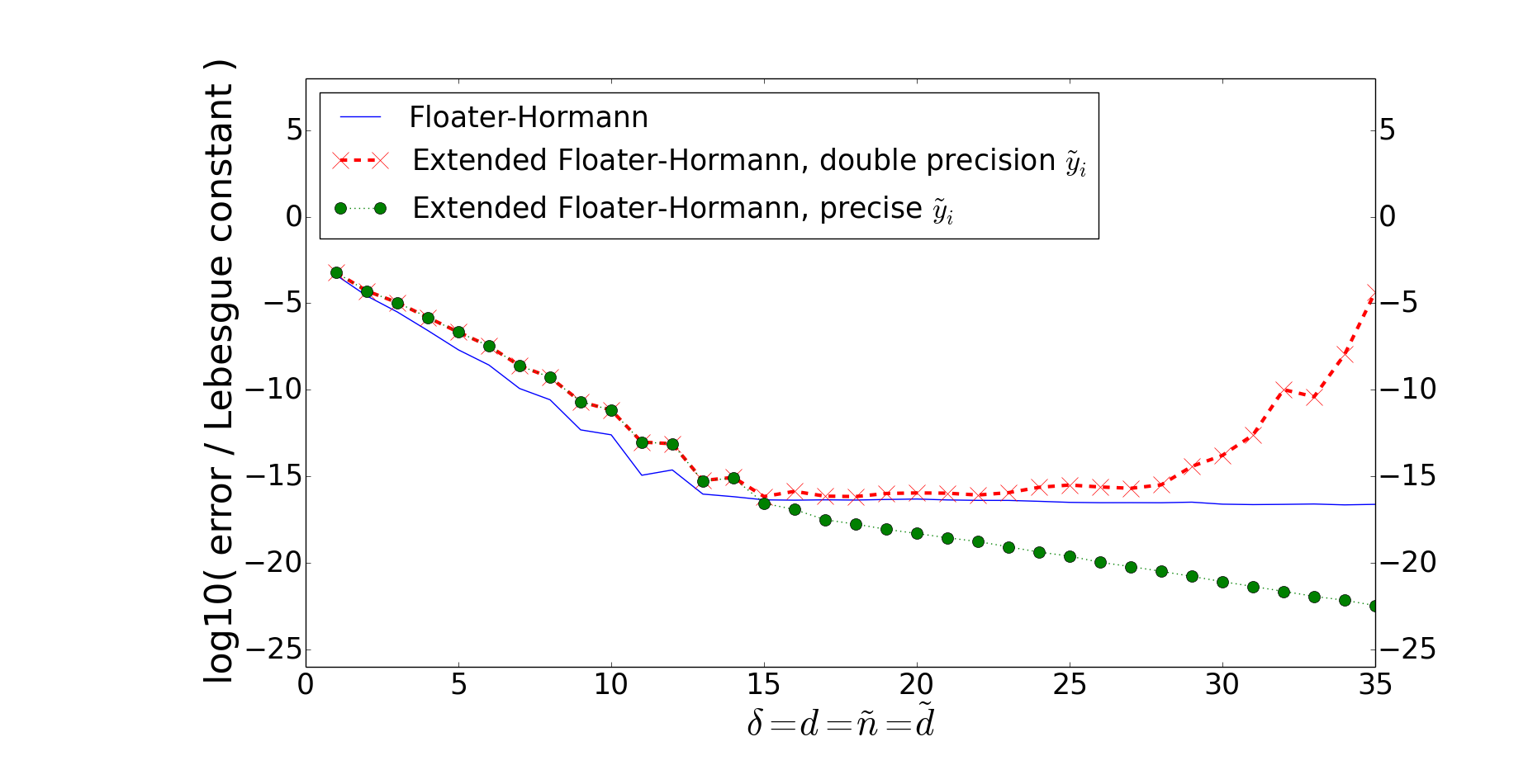
Figure 9: Log10 of (forward error divided by the Lebesgue constant) for ${f}\!\left(t\right)={\sin}\!\left(20t\right)$, $t\in[-1,1]$ and $n=200$.

The data in Figures 5 and 8 are combined in Figure 9, which highlights important points for the case $d=\tilde{n}=\tilde{d}\geq 15$. Note that this case is covered by the theory in BerrutKleinCAM and Klein and their experiments consider $0\leq d\leq 50$. Moreover, extended interpolants are claimed to be better than usual ones for allowing larger values of $d$ and, in view of Figure 7, the use of a larger $\tilde{d}\leq\tilde{n}$ is natural in this context. According to Figure 9,

1. For fixed $n$, the error incurred by usual Floater-Hormann interpolants is of order $n\epsilon\tilde{\Lambda}_{\mathbf{x},\delta}{}\left\|{f}\right\|_{\infty}$.
   

2. For fixed $n$, the error incurred by extended interpolants grows faster than $n\epsilon\tilde{\Lambda}_{\mathbf{x},d,\tilde{n},\tilde{d}}{}\left\|{f}\right\|_{\infty}$ when $d=\tilde{d}=\tilde{n}$.
   

3. The effects of the large Lebesgue constant are reduced when $\tilde{\mathbf{y}}$ is precise. In this case, numerical errors occur mostly in the evaluation of the barycentric formula, and the argument following Equation (3.2) in Klein applies and explains the errors of order $\epsilon$ for the extended interpolants with precise $\tilde{\mathbf{y}}$ in Figure 8.

The data for the extended interpolants with double precision $\tilde{y}_{i}$ in Figure 9 for $d\geq 30$ indicate the existence of another source of numerical instability for these interpolants, in addition to the large Lebesgue constants. This extra source of instability are the enormous entries of the matrices $a_{ij}$ and $b_{ij}$ in Lemma 1, which are defined explicitly in (28)–(29). In fact, Figure 10 shows that the $a_{ij}$ and $b_{ij}$ grow exponentially with $d=\tilde{d}=\tilde{n}$.

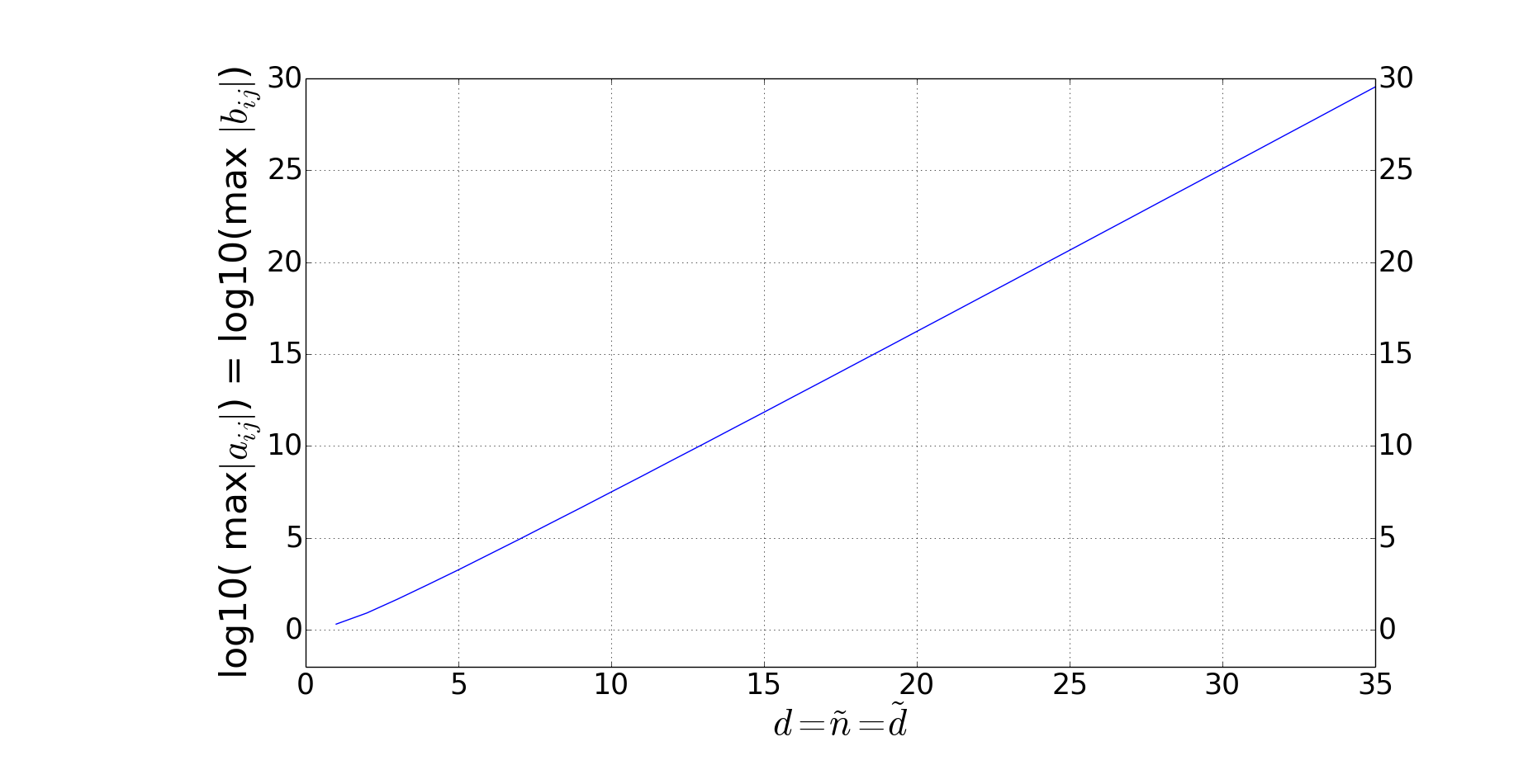
Figure 10: Log10($\max\left|a_{ij}\right|$) = Log10($\max\left|b_{ij}\right|$) for $n=200$.

In view of the remarkable accuracy of the extended interpolants with precise $\tilde{\mathbf{y}}$, it makes sense to consider the possibility of using $\tilde{\mathbf{y}}$ evaluated in multiple precision from the double precision $y_{i}$ which are usually available. These $\tilde{\mathbf{y}}$ are not as precise as the ones obtained from high precision $\mathbf{y}$ using multiple precision arithmetic. Figure 11 illustrates, however, that this strategy improves the accuracy of extended interpolants, at a relatively low cost when $d$, $\tilde{d}$ and $\tilde{n}$ are small compared to $n$ and we want to evaluate the interpolants for many values of $t$.

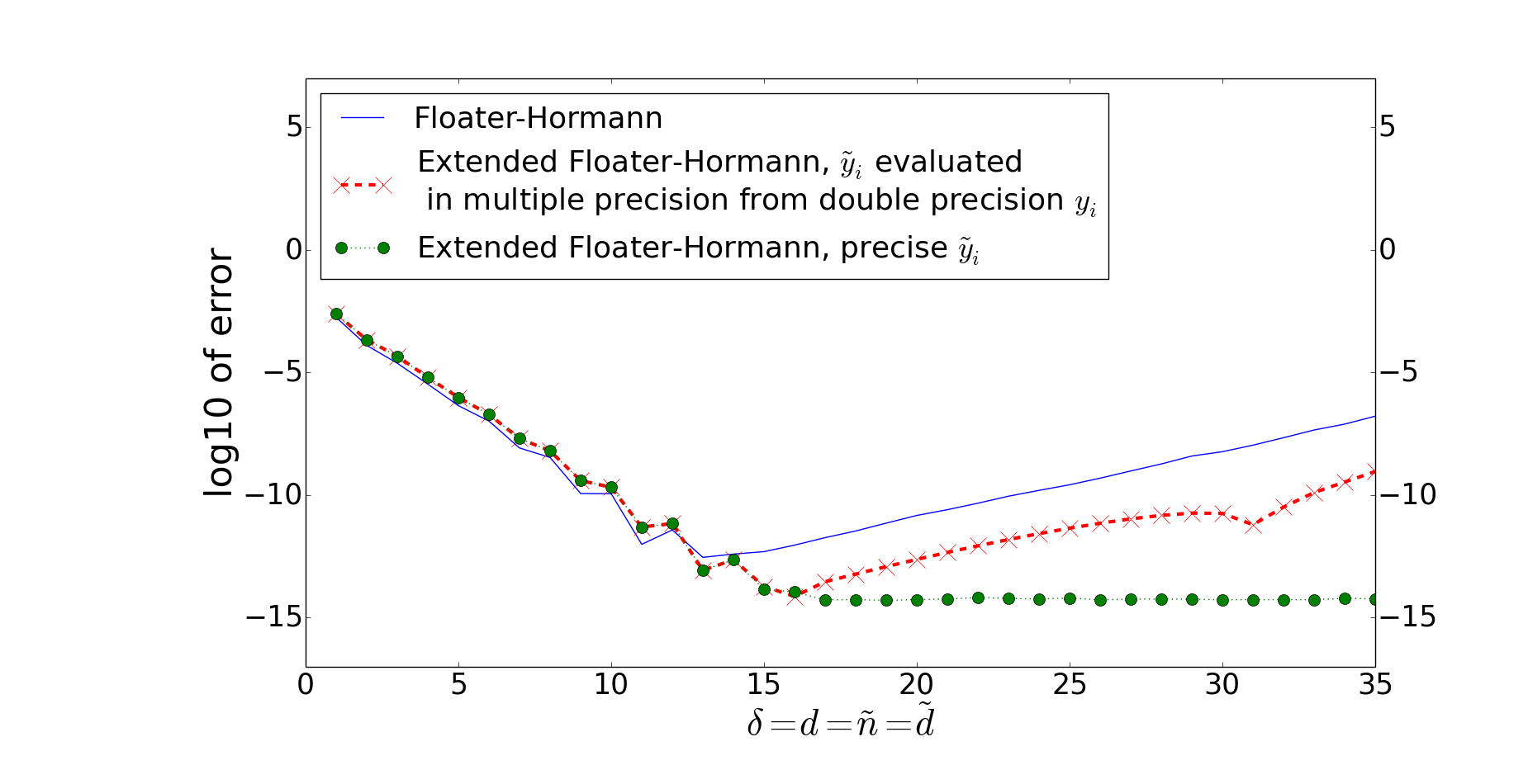
Figure 11: Log10 of the forward error for ${f}\!\left(t\right)={\sin}\!\left(20t\right)$, $t\in[-1,1]$ and $n=200$.

In the case considered in this section, Figure 12 shows that $\tilde{\mathbf{y}}$ evaluated using multiple precision, from double precision $\mathbf{y}$, lead to overall numerical errors of order $n\epsilon\tilde{\Lambda}_{\mathbf{x},d,\tilde{n},\tilde{d}}{}$, which are about 100 times smaller than the errors incurred by the usual Floater-Hormann interpolants in our experiments for large $\delta=d=\tilde{n}=\tilde{d}$.

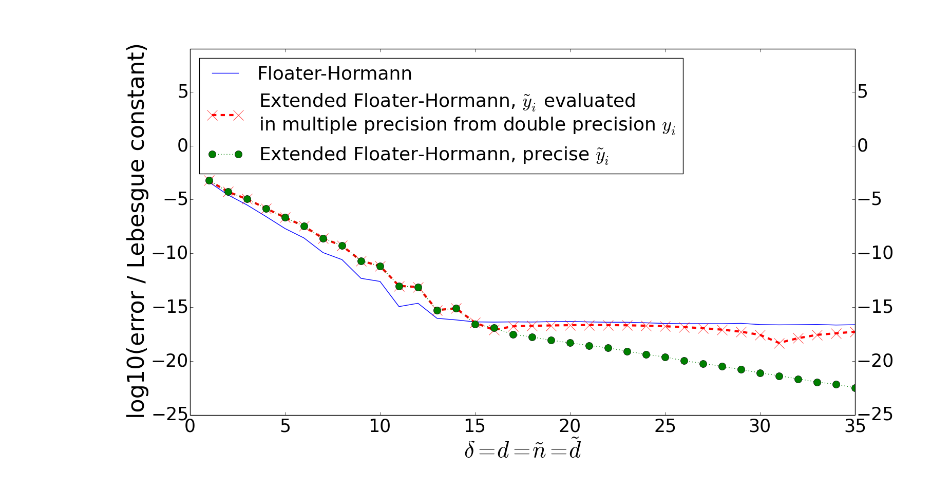
Figure 12: Log10 of (forward error divided by the Lebesgue constant) for ${f}\!\left(t\right)={\sin}\!\left(20t\right)$, $t\in[-1,1]$ and $n=200$.

Appendix A What can we prove about the stability of extended interpolants

This appendix illustrates the difficulties in building a general and realistic stability theory for extended interpolants, a theory which would take into account the errors introduced by the current implementations of floating point arithmetic. We explain that the stability of extended interpolants is sensitive to the way we implement the extrapolation step, and that the accuracy of this step depends on the cancellation of the rounding errors. In fact, the errors incurred by extended interpolants can be enormous when we use the extrapolation formula proposed in BerrutKleinCAM and Klein , and compute $\tilde{\mathbf{y}}$ according to the following procedure:

• If $i$ is even, set the rounding mode upward and evaluate $\tilde{y}_{i}$ as in (6)–(8).

• If $i$ is odd, set the rounding mode downward and evaluate $\tilde{y}_{i}$ as in (6)–(8).

In this scenario the overall effect of rounding errors can be much larger than what one would expect from the already large Lebesgue constants, as illustrated in Figures 13 and 14. In the plots corresponding to $\tilde{\mathbf{y}}$ evaluated as in (10)–(11) in these figures, $\tilde{\mathbf{y}}$ was obtained by matrix multiplication, with $a_{ij}$ and $b_{ij}$ computed in multiple precision and then rounded to double precision i.e., with $a_{ij}$ and $b_{ij}$ as accurate as possible.

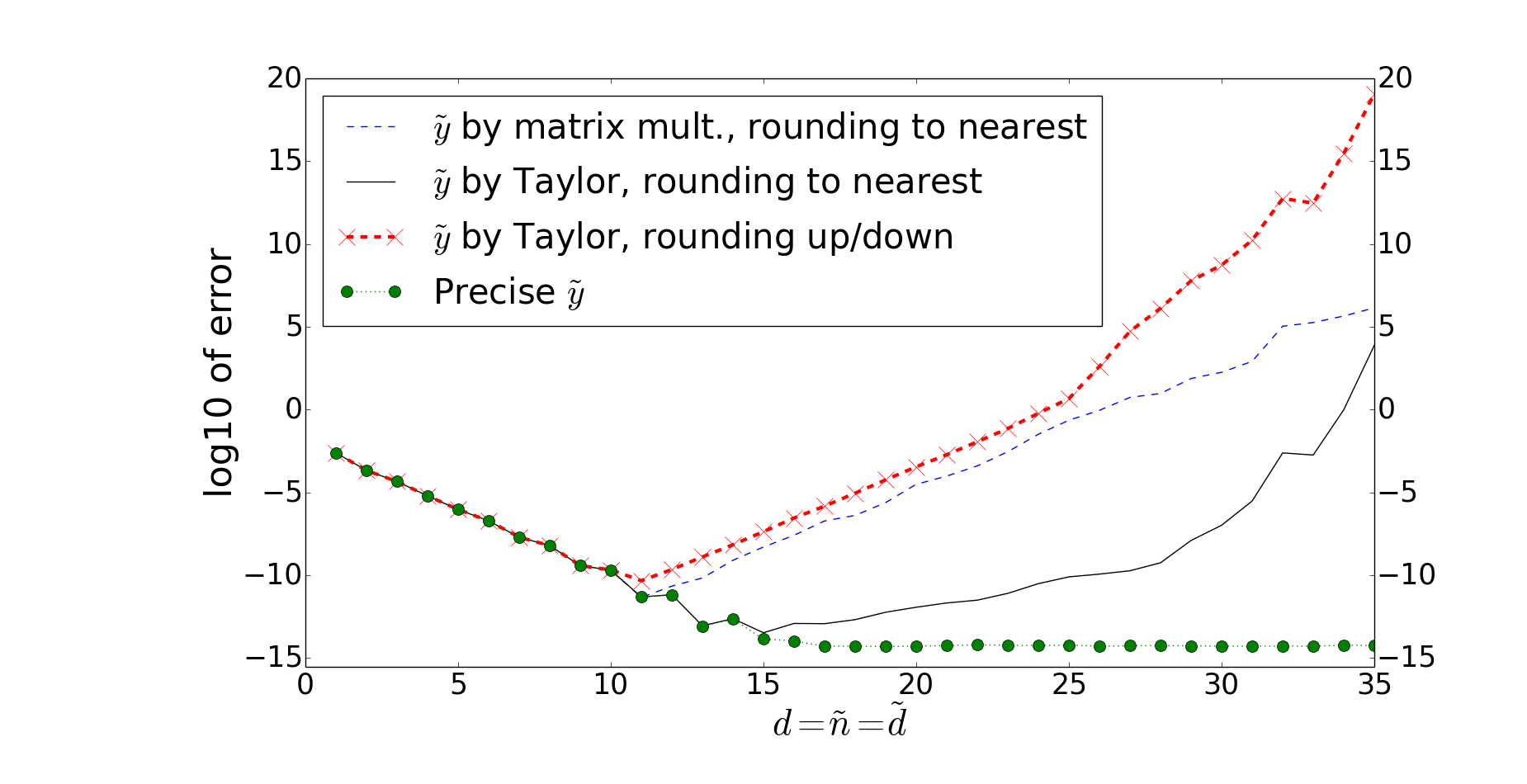
Figure 13: Extended Floater-Hormann. Log10 of the forward error for ${f}\!\left(t\right)={\sin}\!\left(20t\right)$ for $t\in[-1,1]$ and $n=200$. By “$\tilde{y}$ by Taylor” we mean $\tilde{y}$ computed by Taylor series as in BerrutKleinCAM and (6)–(8), and by “$\tilde{y}$ by matrix mult.” we mean $\tilde{y}$ computed by matrix multiplication of $\mathbf{y}$ by the matrices with entries $a_{ij}$ and $b_{ij}$, as in (10)–(11).

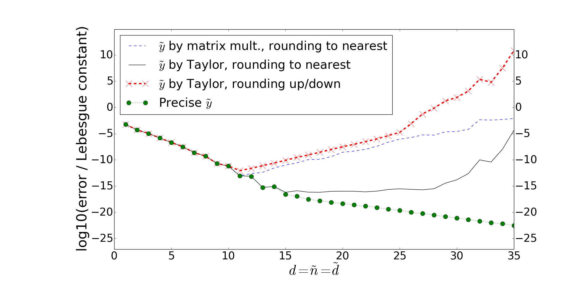
Figure 14: Extended Floater-Hormann. Log10 of (forward error divided by the Lebesgue constant) for ${f}\!\left(t\right)={\sin}\!\left(20t\right)$, $t\in[-1,1]$ and $n=200$.

We emphasize that the choices of rounding modes in the steps (a) and (b) above are not frivolous. Their purpose is to help us understand what can be proved about the numerical stability of extended interpolants, so that we do not try to prove something that cannot be proved. It is unlikely that $\tilde{\mathbf{y}}$ will be evaluated as in the steps (a) and (b) when rounding to nearest. In this mode, there is a 50% chance of rounding up in each flop and, under the questionable hypothesis of independence of the rounding errors, there would be a minuscule probability of $2^{-2\left(d+1\right)d}$ of having all the intermediate results in the evaluation of $\tilde{\mathbf{y}}$ rounded up when rounding to nearest. Since the set of floating point numbers is finite, such a coincidence may be impossible. However, our experiments indicate that it is difficult to build a realistic theory on the effects of rounding errors on extended interpolants, because the rounding errors induced by our changes of rounding modes would be allowed by usual models of floating point arithmetic, with $\epsilon$ replaced by $2\epsilon$. More precisely: when evaluating $\tilde{\mathbf{y}}$, with our choices of rounding modes, we monitored the relative errors

$$\left|\frac{{\mathrm{fl}}\!\left(x+y\right)-\left(x+y\right)}{\left(x+y\right)}\right|\hskip 28.45274pt\mathrm{and}\hskip 28.45274pt\left|\frac{{\mathrm{fl}}\!\left(x*y\right)-\left(x*y\right)}{\left(x*y\right)}\right|$$

for each operation we performed, and found all of them to be smaller than $1.97\epsilon$.

In other words, a stability theory for extended interpolants based on the usual models of floating point arithmetic would need to cover the changes of rounding modes in steps (a) and (b) above and, as a result, its predictions would be too pessimistic. Therefore, a realistic stability theory for extended interpolants will require additional hypothesis regarding the floating point arithmetic. By contrast, under the usual models of floating point arithmetic HIGHAM , we already have realistic theories bounding the rounding errors in terms of $\epsilon$, $n$ and the Lebesgue constant for other barycentric interpolation schemes, as in Andre HIGHAM_IMA Masc MascCam MascCamB .

References

(1) Bochkanov, S., AlgLib, an open source library for numerical computation, available at www.alglib.net.
(2) Berrut, J.-P., and G. Klein,
Recent advances in linear barycentric rational interpolation. Journal of Computational and Applied Mathematics 259 (PART A) (2014) pp. 95–107.
(3) Berrut, J.-P., and L. N. Trefethen, Barycentric Lagrange Interpolation. SIAM J. Num. Anal. 46 (3) (2004) pp. 501–517.
(4) Bos, L., De Marchi, S., Hormann, K., and Klein, G.,
On the Lebesgue constant of barycentric rational interpolation at equidistant nodes.
Numer. Math. 121 (3) (2012) pp. 461–471.
(5) Brutman, L., Lebesgue functions for polynomial interpolation – a survey. Ann. Numer. Math. 4 (1997) pp. 111–127.
(6) de Camargo, A. Pierro, On the numerical stability of Floater-Hormann’s rational interpolant,
Numer. Algorithms, 72(1) (2016) pp 131–152.
(7) Floater, M.S., and Hormann, K., Barycentric rational interpolation with no poles
and high rates of approximation. Numer. Math. 107 (2) (2007) pp. 315–331.
(8) Higham, N. J., The numerical stability of barycentric Lagrange
interpolation, IMA J. Numer. Anal. 24, (2004) pp. 547–556.
(9) Higham, N. J., Accuracy and Stability of Numerical Algorithms, 2nd ed., SIAM, Philadelphia (2002).
(10) Klein, G., An extension of the Floater-Hormann family of barycentric rational interpolants.
Math. Comp. 82 (284) (2013) pp. 2273–2292.
(11) Klein, G. and Berrut, J.-P.,
Linear rational finite differences from derivatives of barycentric rational interpolants.
SIAM J. Numer. Anal. 50 (2) (2012) pp. 643–656.
(12) Mascarenhas, W. F., The stability of barycentric interpolation at the Chebyshev points of the second kind,
Numer. Math., (2014) available online, DOI: 10.1007/s00211-014-0612-6.
(13) Mascarenhas, W. F. and de Camargo, A. Pierro, On the backward stability of the second barycentric formula for interpolation,
Dolomites Res. Notes Approx. 7 (2014) pp. 1–12.
(14) Mascarenhas,W. F. and de Camargo, A. Pierro, The effects of rounding errors in the nodes on barycentric interpolation,
arXiv:1309.7970v2 [math.NA] 4 Jul 2014, submitted to Numer. Math.
(15) Fousse, L., Hanrot, G., Lefèvre, V., Pélissier P., and Zimmermann, P.,
MPFR: A Multiple-Precision Binary Floating-Point Library with Correct Rounding.
ACM Trans. Math. Softw. 33(2), (2007) article 13.
(16) Trefethen, L. N., and Weideman, J.A.C.,
Two results on polynomial interpolation in equally spaced points J. Approx. Theory 65 (1991) pp. 247–260.