Axion Dark Matter Detection using Atomic Transitions

Abstract

Dark matter axions may cause transitions between atomic states that differ in energy by an amount equal to the axion mass. Such energy differences are conveniently tuned using the Zeeman effect. It is proposed to search for dark matter axions by cooling a kilogram-sized sample to milliKelvin temperatures and count axion induced transitions using laser techniques. This appears an appropriate approach to axion dark matter detection in the $10^{-4}$ eV mass range.

Axions provide a solution to the strong CP problem of the Standard Model of elementary particles axion and are a candidate for the dark matter of the universe axdm . Moreover it has been argued recently that axions are the dark matter, at least in part, because they form a rethermalizing Bose-Einstein condensate CABEC and this explains the occurrence of caustic rings of dark matter in galactic halos case . The evidence for caustic rings is summarized in ref.MWhalo . More recently, axion Bose-Einstein condensation was shown to provide a solution to the galactic angular momentum problem Banik . In supersymmetric extensions of the Standard Model, the dark matter may be a mixture of axions and supersymmetric dark matter candidates Baer .

There is excellent motivation then to try and detect axion dark matter. The cavity technique has been used for many years and has placed significant limits in the frequency range 0.46 to 0.86 GHz. [Frequency $f$ is converted to axion mass $m_{a}$ using $2\pi~{}(2.42~{}{\rm GHz})=10^{-5}{\rm eV}$, in units where $\hbar=c=1$.] However, because the axion mass is poorly constrained, one wishes to search over as large a range as possible. The range of the cavity experiment is being extended Shok and other detection methods PDY ; NMR ; LC have been proposed and are being explored but these efforts have not produced limits yet. Here we propose searching for axion dark matter by detecting atomic transitions in which axions are absorbed. Previous authors have considered the use of atoms in the context of axion searches. In ref. ZS it was proposed to detect axions emitted in atomic transitions, using the cavity technique. Ref. Barb proposed to search for dark matter axions by converting them to magnons in a ferromagnet. Ref. Stad proposes to search for the parity violating effects, such as oscillating electric dipole moments, that dark matter axions induce in atoms. However, the specific proposal presented here appears new.

The properties of the axion are mainly determined by the axion decay constant $f_{a}$, which is of order the vacuum expectation value that breaks the $U_{\rm PQ}(1)$ symmetry of Peccei and Quinn. In particular the axion mass

$$m_{a}\simeq 0.6\cdot 10^{-4}{\rm eV}\left({10^{11}~{}{\rm GeV}\over f_{a}}\right)~{}~{}\ .$$ (1)

The axion coupling to fermions has the general form

$${\cal L}_{a\bar{f}f}=-{g_{f}\over 2f_{a}}\partial_{\mu}a~{}\bar{f}(x)\gamma^{\mu}\gamma_{5}f(x)$$ (2)

where $a(x)$ is the axion field and $f(x)$ a fermion field. Of interest here are the couplings to the electron $(f=e)$ and to the nucleons $(f=p,n)$. Eq. (2) ignores small CP violating effects that are unimportant for our purposes. Formulas for the $g_{f}$ are given in refs. Kapl ; Sred . Generically the $g_{f}$ are model-dependent numbers of order one. However the electron coupling $g_{e}$ can readily be set equal to zero at tree level. This is true for example in the KSVZ model KSVZ . In that case, $g_{e}\sim 10^{-3}$ due to a one loop effect Sred . On the other hand, it is unlikely that $g_{p}$ or $g_{n}$ is much less than one because the axion mixes with the neutral pion and therefore its coupling to the nucleons receives a contribution from the pion-nucleon coupling. $g_{p}$ or $g_{n}$ may be much less than one only due to a fortuitous cancellation. It is especially unlikely that both $g_{p}$ and $g_{n}$ are much less than one.

Stellar evolution arguments constrain the couplings under consideration. The coupling to electrons causes stars to emit axions through the Compton-like process $\gamma+e^{-}\rightarrow e^{-}+a$ and through axion bremstrahlung $e^{-}+(Z,A)\rightarrow(Z,A)+e^{-}+a$. The resulting enhanced energy losses in globular cluster stars excessively delay the onset of their helium burning unless ${g_{e}\over f_{a}}\equiv g_{a\bar{e}e}<4.9\cdot 10^{-10}$/GeV Raff . The increase in the cooling rate of white dwarfs due to axion emission provides similar bounds Raff2 . Isern et al. Isern find that the inclusion of axion emission in the white dwarf cooling rate noticeably improves the agreement between theory and observations. Their best fit value is $g_{a\bar{e}e}=2.7\cdot 10^{-10}$/GeV, whereas their upper bound is $g_{a\bar{e}e}<5.5\cdot 10^{-10}$/GeV. The proposal that the white dwarf cooling rate is being modified by axion emssion is testable by the detector described here and provides additional motivation for it. The coupling to nucleons causes axions to be radiated by the collapsed stellar core produced in a supernova explosion. The requirement that the observed neutrino pulse from SN1987a not be quenched by axion emission implies $f_{a}>4\cdot 10^{8}$ GeV SN1987a ; Raff3 . Using Eq. (1), this is equivalent to $m_{a}<1.6\cdot 10^{-2}$ eV.

The couplings under consideration are also constrained by laboratory searches. Limits on $g_{aee}$ have been obtained gaee by searching for solar axions using the axio-electric effect in a laboratory target Dimop . A limit on the product $g_{a\gamma\gamma}g_{a\bar{e}e}$, where $g_{a\gamma\gamma}$ is the coupling of the axion to photons, was obtained CASTgaee by searching for the conversion of solar axions to x-rays in a laboratory magnetic field axdet .

In the non-relativistic limit, Eq. (2) implies the interaction energy

$$H_{a\bar{f}f}=+{g_{f}\over 2f_{a}}\left(\vec{\nabla a}\cdot\vec{\sigma}+\partial_{t}a~{}{\vec{p}\cdot\vec{\sigma}\over m_{f}}\right)$$ (3)

where $m_{f}$ is the mass of fermion $f$, $\vec{p}$ its momentum and $\vec{S}={1\over 2}\vec{\sigma}$ its spin. The first term on the RHS of Eq. (3) is similar to the coupling of the magnetic field to spin, with $\vec{\nabla}a$ playing the role of the magnetic field. That interaction causes magnetic dipole (M1) transitions in atoms. The second term causes $\Delta j=0$, $\Delta l=1$, parity changing transitions. As usual, $l$ is the quantum number giving the magnitude of orbital angular momentum, and $j$ that of total angular momentum. We will not use the second term because, starting from the ground state ($l=0$), it causes transitions only if the energy absorbed is much larger than the axion mass. If $f=e$, the required energy is of order eV. If $f=p,n$, the required energy is of order MeV.

The ground state of most atoms is accompanied by several other states related to it by flipping the spin of one or more valence electrons, or by changing the $z$-component $I_{z}$ of the nuclear spin. The energy differences between these states can be conveniently tuned by the Zeeman effect. The interaction of the axion with a nuclear spin $\vec{I}$ may be written

$$H_{a\bar{N}N}={g_{N}\over f_{a}}\vec{\nabla}a\cdot\vec{I}$$ (4)

where the $g_{N}$ are dimensionless couplings of order one that are determined by nuclear physics in terms of $g_{p}$ and $g_{n}$. Relevant calculations are presented in ref. Flam .

The transition rate by axion absorption from an atomic ground state $|0>$ to a nearby excited state $|i>$ is

$$R_{i}={1\over 2m_{a}f_{a}^{2}} \min(t,t_{1},t_{a})\cdot$$

$$~{}\cdot\int d^{3}p~{}~{}{d^{3}n\over dp^{3}}(\vec{p}) |<i|(g_{e}\vec{S}+g_{N}\vec{I})\cdot\vec{p}|0>|^{2}$$ (5)

on resonance. Here and henceforth $\vec{S}$ is electron spin. $t$ is the measurement integration time, $t_{1}$ is the lifetime of the excited state, and $t_{a}$ is the coherence time of the signal. The latter is set by the energy dispersion $\delta E=m_{a}(1+{1\over 2}\overline{v^{2}})$ of dark matter axions, where $\overline{v^{2}}$ is their average velocity squared. The frequency spread of the axion signal is $B_{a}=t_{a}^{-1}={\delta E\over 2\pi m_{a}}$. The resonance condition is $m_{a}=E_{i}-E_{0}$ where $E_{i}$ and $E_{0}$ are the energies of the two states. The detector bandwidth, i.e. the frequency spread over which resonant transitions occur, is $B=1/\min(t,t_{1})$. ${d^{3}n\over dp^{3}}(\vec{p})$ is the local axion momentum distribution. The local axion energy density is

$$\rho_{a}=m_{a}\int d^{3}p~{}{d^{3}n\over dp^{3}}(\vec{p})~{}~{}\ .$$ (6)

Let us define $g_{i}$ by

$$g_{i}^{2}\overline{v^{2}}m_{a}\rho_{a}\equiv\int d^{3}p~{}{d^{3}n\over dp^{3}}(\vec{p})|<i|(g_{e}\vec{S}+g_{N}\vec{I})\cdot\vec{p}|0>|^{2}~{}~{}\ .$$ (7)

$g_{i}$ is a number of order one giving the coupling strength of the target atom. It depends on the atomic transition used, the direction of polarization of the atom, and the momentum distribution of the axions. It varies with time of day and of year since the momentum distribution changes on those time scales due to the motion of the Earth.

For a mole of target atoms, the transition rate on resonance is

$$N_{A}R_{i}=g_{i}^{2}N_{A}~{}\overline{v^{2}}~{}{2\rho_{a}\over f_{a}^{2}}\min(t,t_{1},t_{a})$$

$$=~{}{535\over{\rm sec}}\left({\rho_{a}\over{\rm GeV}/{\rm cm}^{3}}\right)\left({10^{11}~{}{\rm GeV}\over f_{a}}\right)^{2}\cdot$$

$$~{}\cdot g_{i}^{2}~{}\left({\overline{v^{2}}\over 10^{-6}}\right)\left({\min(t,t_{1},t_{a})\over{\rm sec}}\right)$$ (8)

where $N_{A}$ is Avogadro’s number. There is an (almost) equal transition rate for the inverse process, $|i>\rightarrow|0>$ with emission of an axion. It is proposed to allow axion absorptions only by cooling the target to a temperature $T$ such that there are no atoms in the excited state. The requirement $N_{A}e^{-m_{a}\over T}<0.1$ implies

$$T=12~{}{\rm mK}\left({10^{11}~{}{\rm GeV}\over f_{a}}\right)~{}~{}\ .$$ (9)

The transitions are detected by shining a tunable laser on the target. The laser’s frequency is set so that it causes transitions from state $|i>$ to a highly excited state (with energy of order eV above the ground state) but does not cause such transitions from the ground state or any other low-lying state. When the atom de-excites, the associated photon is counted. The efficiency of this technique for counting atomic transitions is between 50% and 100%.

Consider a sweep in which the frequency is shifted by the bandwidth $B$ per measurement integration time $t$. The number of events per tune on resonance is $tN_{A}R_{i}$. If $B_{a}<B$, events occur only during one tune, whereas events occur during $B_{a}/B$ successive tunes if $B_{a}>B$. Thus the total number of events per mole during a sweep through the axion frequency $\nu_{a}=m_{a}/2\pi$ is

$${\#{\rm events}\over{\rm mole}}=tN_{A}R_{i}{\min(t,t_{1})\over\min(t,t_{1},t_{a})}~{}~{}\ .$$ (10)

To proceed at a reasonably fast pace, the search should cover a frequency range of order $\nu_{a}$ per year. Assuming a 30% duty cycle, one needs

$${B\over t}={1\over t\min(t,t_{1})}={\nu_{a}\over 0.3~{}{\rm year}}={1.5~{}{\rm kHz}\over{\rm sec}}\left({10^{11}~{}{\rm GeV}\over f_{a}}\right)~{}~{}\ .$$ (11)

The expected number of events per sweep through the axion frequency is then

$${\#{\rm events}\over{\rm mole}} = 0.35~{}g_{i}^{2}~{}\left({\overline{v^{2}}\over 10^{-6}}\right)\cdot$$ (12)

$$\cdot \left({\rho_{a}\over{\rm GeV}/{\rm cm}^{3}}\right)\left({10^{11}~{}{\rm GeV}\over f_{a}}\right)~{}\ .$$

Note that, when the constraint of Eq. (11) is satisfied, the number of events per sweep through the axion frequency is independent of $t$, $t_{1}$ and $t_{a}$.

The actual number of events has a Poisson probability distribution whose average is given by Eq. (12). Let $\epsilon$ be the efficiency for counting an actual event. We assume that each counted event is checked to see whether it is due to axions or to something else, by staying at the same tune for a while and verifying whether additional events occur and what is their cause. If $N$ is the expected number of events, and the events are Poisson distributed, the probability to have at least one event counted is $~{}1-e^{-\epsilon N}$. To obtain a 95% confidence level (CL) upper limit, one needs therefore $N>3/\epsilon$. Hence Eq. (12) implies that, in the absence of an axion detection, the 95% CL upper limit from a sweep through the axion frequency is

$$g_{i}<3.0 \sqrt{\left({1\over\epsilon}\right)\left({A~{}{\rm gr}\over M}\right)\left({10^{-6}\over\overline{v^{2}}}\right)}\cdot$$ (13)

$$\cdot \sqrt{\left({{\rm GeV/cm}^{3}\over\rho_{a}}\right)\left({f_{a}\over 10^{11}~{}{\rm GeV}}\right)}$$

where $M$ is the total mass of target material and $A$ its atomic number per target atom.

Figure 1: Expected sensitivity of the proposed detector to the coupling of the axion to electrons. The diagonal lines are the predictions of models with $g_{e}$ = 1.0 and 0.3. The vertical line on the right is an upper bound on the axion mass from supernova SN1987a. The solid horizontal line is an upper limit on the coupling from the white dwarf cooling rate. The horizontal dotted line is the value of the coupling that yields a best fit to the white dwarf cooling observations. The shaded area indicates the expected sensitivity of the proposed detector under the assumptions spelled out in the text, using electron paramagnetic resonance (dark) and anti-ferromagnetic resonance (light)

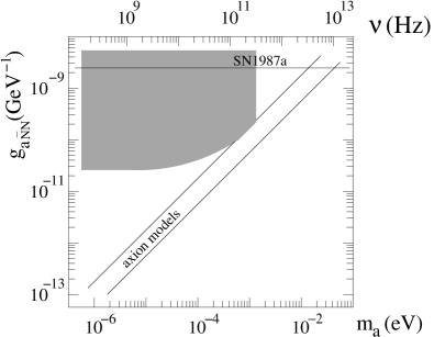
Figure 2: Expected sensitivity of the proposed detector to the coupling of the axion to nuclei. The diagonal lines are the couplings when $g_{N}$ = 1.0 and 0.3. The horizontal line near the top is the upper bound on the coupling from supernova SN1987a, for $g_{N}$ =1. The shaded area indicates the expected sensitivity of the proposed detector under the assumptions spelled out in the text.

A suitable target material may be found among the numerous salts of transition group ions that have been studied extensively using electron paramagnetic resonance techniques Altshuler ; Abragam . The low energy states of such ions time-evolve according to a Hamiltonian of the general type:

$$H(\vec{S},\vec{I})=-\gamma\vec{S}\cdot\vec{\cal H}-\gamma_{N}\vec{I}\cdot\vec{\cal H}+U\vec{S}\cdot\vec{I}+P[I_{z}^{2}-{1\over 2}(I_{x}^{2}+I_{y}^{2})]$$ (14)

where $\vec{\cal H}$ is the magnetic field. The term with coefficient $U$ is responsible for hyper-fine structure. ($U$ is commonly called $A$ in the litterature but we already use $A$ to mean atomic number). The term with coefficient $P$ results from the interaction of the nuclear electric quadrupole moment with the crystalline field. We assumed cubic symmetry for simplicity and ignored possible terms that are non-linear in $S$. Let us first discuss searches for a coupling of axion dark matter to electron spin. The first term on the RHS of Eq. (14), involving the electron gyromagnetic ratio $\gamma\simeq\mu_{B}\simeq(2\pi)14.0$ GHz/T, allows such a search up to frequencies of order 280 GHz assuming that the maximum ${\cal H}$ is 20 T. To estimate the search sensitivity, it is necessary to make assumptions. We assume $\rho_{a}$ = 1 GeV/cm³ and $\bar{v^{2}}$ = 10^-6, based on the halo model of ref. MWhalo . We assume further that a suitable material is found with $A$ = 150 or smaller, that the mass of such material that can be cooled to temperature $T$ is $M=1{\rm kg}~{}({T\over{\rm mK}})$, and that the detection efficiency $\epsilon=0.6$. Eq. (13) implies then $g_{i}<0.4~{}({f_{a}\over 10^{11}~{}{\rm Gev}})$. Furthermore, we assume $I=0$ and that the axion momentum is randomly oriented relative to the direction of polarization of the target. Eq. (7) implies then $g_{i}={1\over 2}\sqrt{2\over 3}g_{e}$. The dark grey area in Fig. (1) shows the 95% CL upper limit on $g_{a\bar{e}e}={g_{e}\over f_{a}}$ that would be obtained under these assumptions. The search may be extended to higher frequencies by using resonant transitions in anti-ferromagnetic materials. The resonant frequencies are high (e.g. 1.58 THz in the case of FeF₂) due to the high effective magnetic fields at the location of the electron spin in the crystal. The resonant frequency can be tuned over some range by applying an external magnetic field. Assuming suitable target materials can be found, the search for a coupling of dark matter axions to electron spin can be extended upwards in frequency as indicated by the light shaded area in Fig. 1.

Next let us discuss a search for the coupling of dark matter axions to nuclear spin. The second term in Eq. (14), involving the nuclear gyromagnetic ratio $\gamma_{N}$, allows only a small tuning range, of order 150 MHz, since the nuclear magneton $\mu_{N}\simeq(2\pi)$ 7.62 MHz/T. However, a large tuning range can be obtained by exploiting the penultimate term in Eq. (14) since, for some salts of rare earth ions, $U$ is if order $2\pi$ (GHz) to $2\pi$ (10 GHz). The diagonalization of $H(\vec{S},\vec{I})$ is straightforward and discussed in textbooks. It is also straightforward to calculate the matrix elements between the energy eigenstates for the absorption of an axion. From the groundstate, the selection rules for axion-induced transitions allow transitions to three different excited states if $I>1/2$, two if $I=1/2$. Transitions are always possible to the highest energy eigenstate, the one in which $S_{z}=1/2$ and $I_{z}=I$ in case $\vec{\cal H}={\cal H}\hat{z}$ and $U>0$, as we assume henceforth. As it provides the largest tuning range , we focus on that particular transition. For the sake of simplicity, we set $\gamma_{N}=P=0$. The corrections from finite $\gamma_{N}$ and $P$, as well as from other terms that may be present on the RHS of Eq. (14), are readily included but they do not change the qualitative picture. The resonant frequency for the stated transition is $E_{i}-E_{0}={1\over 2}(-\gamma{\cal H}+(I+{1\over 2})U)+\sqrt{{1\over 4}(-\gamma{\cal H}+(I-{1\over 2})U)^{2}+{1\over 2}U^{2}I}$. For the sake of estimating the sensitivity, we set $g_{e}=0$. If a signal is found it is possible to measure $g_{e}$ and $g_{N}$ separately by using a variety of target atoms and by exploiting the fact that there are two or three transitions per target atom. The relevant matrix element squared is then

$$|<i|\vec{I}\cdot\vec{p}|0>|^{2}={1\over 2}I(p_{x}^{2}+p_{y}^{2}){\beta\over 1+2\beta+\sqrt{1+2\beta}}$$ (15)

where $\beta\equiv I({U\over-\gamma{\cal H}+(I-1/2)U})^{2}$. $g_{i}={\cal O}(1)$ over a tuning range of order $IU$. The largest available range appears to be afforded by the ${}^{165}H_{o}$ nucleus which has $I$ = 7/2 and $U=2\pi$(10.5) GHz in diluted trichloride salts Abragam . Assuming these values and $A=10^{3}$, and keeping all other assumptions the same as for the $g_{a\bar{e}e}$ sensitivity curve, results in the $g_{a\bar{N}N}\equiv{g_{N}\over f_{a}}$ sensitivity curve shown in Fig. 2.

I am grateful to Guido Mueller, Gray Rybka, Tarek Saab, Neil Sullivan and David Tanner for useful discussions. This work was supported in part by the U.S. Department of Energy under Grant No. DE-FG02-97ER41029 at the University of Florida and by the National Science Foundation under Grant No. PHYS-1066293 at the Aspen Center for Physics.

References

- (1) R. D. Peccei and H. Quinn, Phys. Rev. Lett. 38 (1977) 1440 and Phys. Rev. D16 (1977) 1791; S. Weinberg, Phys. Rev. Lett. 40 (1978) 223; F. Wilczek, Phys. Rev. Lett. 40 (1978) 279.
- (2) J. Preskill, M. Wise and F. Wilczek, Phys. Lett. B120 (1983) 127; L. Abbott and P. Sikivie, Phys. Lett. B120 (1983) 133; M. Dine and W. Fischler, Phys. Lett. B120 (1983) 137.
- (3) P. Sikivie and Q. Yang, Phys. Rev. Lett. 103 (2009) 111301.
- (4) P. Sikivie, Phys. Lett. B695 (2011) 22.
- (5) L.D. Duffy and P. Sikivie, Phys. Rev. D78 (2008) 063508.
- (6) N. Banik and P. Sikivie, Phys. Rev. D88 (2013) 123517.
- (7) H. Baer, AIP Conf. Proc. 1604 (2014) 289, and references therein.
- (8) P. Sikivie, Phys. Rev. Lett. 51 (1983) 1415 and Phys. Rev. D32 (1985) 2988.
- (9) S. Asztalos et al., Phys. Rev. Lett. 104 (2010) 041301, and references therein.
- (10) T.M. Shokair et al., Int. J. of Mod. Phys. A 29 (2014) 1443004.
- (11) P. Sikivie, D.B. Tanner and Y. Wang, Phys. Rev. D50 (1994) 4744; G. Rybka and A. Wagner, arXiv:1403.3121.
- (12) P. Graham and S. Rajendran, Phys. Rev. D88 (2013) 035023; D. Budker et al., Phys. Rev. X 4 (2014) 021030.
- (13) P. Sikivie, N. Sullivan and D.B. Tanner, Phys. Rev. Lett. 112 (2013) 131301.
- (14) K. Zioutas and Y. Semertzidis, Phys. Lett. A130 (1988) 94.
- (15) R. Barbieri et al. Phys. Lett. B226 (1989) 357
- (16) Y.V. Stadnik and V.V. Flambaum, Phys. Rev. D89 (2014) 043522.
- (17) D.B. Kaplan, Nucl. Phys. B260 (1985) 215;
- (18) M. Srednicki, Nucl. Phys. B260 (1985) 689.
- (19) J. Kim, Phys. Rev. Lett. 43 (1979) 103; M. A. Shifman, A. I. Vainshtein and V. I. Zakharov, Nucl. Phys. B166 (1980) 493.
- (20) G. Raffelt and A. Weiss, Phys. Rev. D51 (1995) 1495; M. Catelan, J.A. de Freitas Pacheco and J.E. Horvath, Astroph. J. 461 (1996) 231.
- (21) G. Raffelt, Phys. Lett. B166 (1986) 402; S.I. Blinnikov and N.V. Dunina-Barskovskaya, Mon. Not. R. Astr. Soc. 266 (1994) 289.
- (22) J. Isern et al., Astroph. J. 682 (2008) L109.
- (23) J. Ellis and K. Olive, Phys. Lett. B193 (1987) 525; G. Raffelt and D. Seckel, Phys. Rev. Lett. 60 (1988) 1793; M. Turner, Phys. Rev. Lett. 60 (1988) 1797; H.-T. Janka et al., Phys. Rev. Lett. 76 (1996) 2621; W. Keil et al., Phys. Rev. D56 (1997) 2419.
- (24) G. Raffelt, Lect. Notes Phys. D79 (2008) 51.
- (25) E. Aprile et al., Phys. Rev. D90 (2014) 062009; F.T. Avignone et al., Phys. Rev. D35 (1987) 2752; A. Ljubicic et al., Phys. Lett. B599 (2004) 143.
- (26) S. Dimopoulos, G.D. Starkman and B.W. Lynn, Phys. Lett. B168 (1986) 145.
- (27) K. Barth et al., JCAP 05 (2013) 010.
- (28) Y.V. Stadnik and V.V. Flambaum, arXiv:1408.2184.
- (29) S.A. Altshuler and B.M. Kozyrev, Electron Paramagnetic Resonance, FTD-TT-62-1086/1+2, Moscow, 1961.
- (30) A. Abragam and B. Bleany, Electronic Paramagnetic Resonance of Transitions Ions, Oxford University Press, 1970.