The asymptotic behaviour of the discrete holomorphic map $Z^{a}$ via the Riemann-Hilbert method

Abstract

We study the asymptotic behavior of the discrete analogue of the holomorphic map $z^{{a}}$. The analysis is based on the use of the Riemann-Hilbert approach. Specifically, using the Deift-Zhou nonlinear steepest descent method we prove the asymptotic formulae which was conjectured in 2000 by the first co-author and S.I. Agafonov.

1 Introduction.

The nonlinear theory of discrete complex analysis goes back to 1985 Thurston’s talk [28] at Purdue University and declares circle patterns to be natural discrete analogs of analytic functions [26, 27]. The word “nonlinear” refers to the basic feature of equations describing circle patterns. Often, the so-called cross-ratio system is used for this. In [8] a discrete conformal map was defined as a complex valued function on the square grid $f:\mathbb{Z}^{2}\to\mathbb{R}^{2}=\mathbb{C}$ with the property that the cross ratio on each elementary quadrilateral is -1:

$$\frac{(f_{n,m}-f_{n+1,m})(f_{n+1,m+1}-f_{n,m+1})}{(f_{n+1,m}-f_{n+1,m+1})(f_{n,m+1}-f_{n,m})}=-1.$$ (1.1)

Here and below we abbreviate $f_{n,m}=f(n,m)$. The boundary data $f(n,0),f(0,m)$ and the evolution equation (1.1) determine the whole map uniquely. A discrete conformal map is called embedded if the interiors of different elementary quadrilaterals are disjoint.

Note that the definition of a discrete conformal map is Möbius invariant and is motivated by the following characterization for smooth mappings: A smooth map $f:D\to{\mathbb{C}}$ is conformal (holomorphic or antiholomorphic) if and only if $\forall z\in D\subset{\mathbb{C}}$

$$\lim_{\epsilon\to 0}\frac{(f(z)-f(z+\epsilon)(f(z+\epsilon+i\epsilon)-f(z+i\epsilon))}{(f(z+\epsilon)-f(z+\epsilon+i\epsilon))(f(z+i\epsilon)-f(z))}=-1.$$

It is a very appealing problem to find discrete conformal maps corresponding to classical holomorphic functions. In the following we discuss a discretization of the holomorphic map $z^{a}$. A naive way to construct a discrete analogue of the holomorphic map $z^{a}$ would be to take (1.1) with the boundary data $f(n,0)=n^{2/3}$ and $f(0,m)=(im)^{2/3}$. However, as demonstrated in Figure 1(left), the resulting lattice is not embedded and is far from its continuous counterpart. Hence this map cannot be treated as a discrete $z^{a}$.

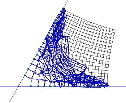
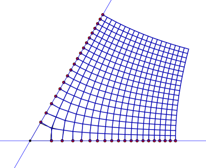
Figure 1: Two discrete conformal maps with close initial data $n=0,m=0$: (Left) Continuous holomorphic mapping $z^{2/3}$ and the discrete holomorphic mapping with the “naive” boundary data $f(n,0)=n^{2/3}$ and $f(0,m)=(im)^{2/3}$. (Right) The discrete $Z^{2/3}$: the boundary data is slightly different from the “naive” ones. [Images by J. Richter-Gebert]

The discrete embedded analog, $Z^{a}$, of the function $z^{a}$ exists and is shown in Figure 1(right). To construct discrete $Z^{a}$ more involved methods coming from the theory of integrable systems are required. Indeed, a crucial property of equation (1.1) is its integrability [24, 8]. In the following we summarize some known facts about the discrete conformal map $Z^{a}$, see [9, 3, 6] for more details.

The discrete map $Z^{a}$ was introduced in [6]. In order to construct an embedded discrete analog of $z^{a}$ the following approach is used. Equation (1.1) can be supplemented with the nonautonomous constraint

$$af_{n,m}=2n\frac{(f_{n+1,m}-f_{n,m})(f_{n,m}-f_{n-1,m})}{(f_{n+1,m}-f_{n-1,m})}+2m\frac{(f_{n,m+1}-f_{n,m})(f_{n,m}-f_{n,m-1})}{(f_{n,m+1}-f_{n,m-1})}.$$ (1.2)

This constraint is derived within the theory of integrable systems. Solutions of (1.1) satisfying (1.2) are singled out by an auxiliary special Fuchsian system, which yields formula (1.2) (see Section 2 and [6, 3] for more details). This constraint is compatible with (1.1). A proof of the compatibility based on the analysis of the corresponding Lax representation and the above mentioned Fuchsian system is given in [9].

We assume that $0<a<2$ and denote $\mathbb{Z}^{2}_{+}=\{(n,m)\in\mathbb{Z}:n,m\geqslant 0\}$. To demonstrate that the constraint (1.2) indeed corresponds to a discrete $Z^{a}$ we investigate its continuous limit. The right hand side of (1.2) in the limit $\epsilon\to 0$ for $z=x+iy=\epsilon(n+im)$ gives

$$\lim_{\epsilon\to 0}2\frac{x}{\epsilon}\frac{(f(z+\epsilon)-f(z))(f(z)-f(z-\epsilon))}{f(z+\epsilon)-f(z-\epsilon)}+2\frac{y}{\epsilon}\frac{(f(z+i\epsilon)-f(z))(f(z)-f(z-i\epsilon))}{f(z+i\epsilon)-f(z-i\epsilon)}=xf_{x}+yf_{y}=zf_{z},$$

where we have used the holomorphicity of the limiting mapping. The corresponding limit of (1.2) becomes $af=zf_{z}$, and its general solution is $f(z)=z^{a}$ up to scaling.

This consideration and the properties $z^{a}(\mathbb{R}_{+})=\mathbb{R}_{+}$ and $z^{a}(i\mathbb{R}_{+})=e^{a\pi i/2}\mathbb{R}_{+}$ of the holomorphic mapping $z^{a}$ motivate the following definition [6] of its discrete analog.

Definition 1

For $0<a<2$ the dicsrete conformal map $Z^{a}:\mathbb{Z}_{+}^{2}\to\mathbb{C}$ is the solution of equations (1.1) and (1.2) with the initial conditions

$$Z^{a}(0,0)=0,\quad Z^{a}(1,0)=1,\quad Z^{a}(0,1)=e^{a\pi i/2}.$$ (1.3)

The properties $Z^{a}(n,0)\in\mathbb{R}_{+}$ and $Z^{a}(0,m)\in e^{a\pi i/2}\mathbb{R}_{+}$ are obvious. The existence of this map was proven using the methods of the theory of integrable systems.

As it was shown in [3], the discrete conformal map $Z^{a}$ determines a circle pattern of Schramm type, i.e. an orthogonal circle pattern with the combinatorics of the square grid. The points $Z^{a}(n,m)$ with even and odd $n+m$ are the centers of the circles and their intersection points respectively (see Figure 2). Moreover, this discrete conformal mapping was also proven to be immersed, i.e. the neighboring elementary quadrilaterals do not overlap. Finally the embeddedness of this mapping was proven in [1].

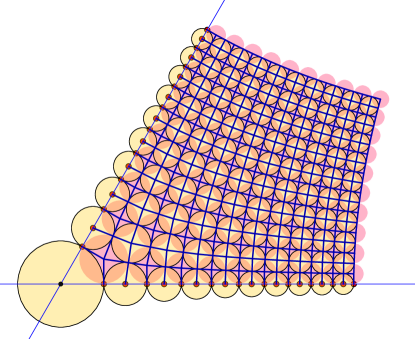
Figure 2: The discrete $z^{2/3}$ as an infinite orthogonal circle pattern: one sector and the covering of the plane. [Images by J. Richter-Gebert and T. Hoffmann]

It turns out that the orthogonal $Z^{a}$-circle pattern can be defined in a pure geometric way without referring to integrable equations. The corresponding rigidity result was obtained in [10] by analysis methods. It reads as follows. For $a\in(0,2)$ the infinite orthogonal circle pattern corresponding to the discrete conformal mapping $Z^{a}$ is the unique embedded orthogonal circle pattern (up to global scaling) with the following two properties (see Figure 2(left)):

• The union of the corresponding kites (elementary quadrilaterals) of the $Z^{a}$-circle pattern covers the infinite sector $\{z=re^{i\phi}\in\mathbb{C}:r\geqslant 0,\phi\in[0,a\pi/2]\}$ with angle $a\pi/2$.

• The centers of the boundary circles lie on the boundary half lines $\mathbb{R}_{+}$ and $e^{a\pi i/2}\mathbb{R}_{+}$.

For rational $a=\frac{4}{N},\ N\in\{2,3\ldots\}$ the rigidity of $Z^{a}$ follows from the rigidity results obtained in [18]. For example for the infinite circle pattern in Figure 2(right) it reads as follows. Consider an orthogonal circle pattern with the combinatorics shown in this figure, i.e. there is one circle intersected by six neighboring circles and all other circles have exactly four intersecting neighbors. Then an orthogonal embedded circle pattern that covers the whole plane and possesses the described combinatorics is unique.

Our goal is to prove the following asymptotic behavior of $f_{n,m}\equiv Z^{a}_{n,m}$ as $n,m\to\infty$, which was conjectured in [3].

Theorem 1

Let $Z^{a}_{n,m}$ be the above defined discrete analog of the power function $z^{a}$. Assume that $0<a<2$. Then,

$$Z^{a}_{n,m}=c(a)\left(\frac{n+im}{2}\right)^{a}\left(1+O\left(\frac{1}{n^{2}+m^{2}}\right)\right),\quad n^{2}+m^{2}\to\infty,$$ (1.4)

with

$$c(a)=\frac{\Gamma\left(1-\frac{a}{2}\right)}{\Gamma\left(1+\frac{a}{2}\right)}.$$

This asymptotics was proven for $n=0,1$ in [3]. Also by elementary methods the corresponding asymptotics without a formula for $c(a)$ was proven for $n-m={\rm const}$ in [2].

Theorem 1 is the statement about the asymptotics of the solution of the Cauchy problem for equations (1.1) and (1.2) determined by the initial data (1.3). Equations (1.1) and (1.2) are nonlinear difference equations. It is difficult, if not impossible, unless solution is explicit or given in terms of contour integrals, to perform global asymptotic analysis of nonlinear equations, both difference and differential. The reason we are able to do this in the case of the Cauchy problem for equations (1.1) and (1.2) is their integrability. The latter allows us to use the Riemann-Hilbert approach - a noncomutative analog of contour integral representation and apply the nonlinear steepest descent method of Deift and Zhou [13] in our investigation.

As it will be shown in the main text, the function $Z^{a}_{n,m}$ is intimately related to a certain collection of orthogonal polynomials. Hence the necessity to use the orthogonal polynomial version of the Deift-Zhou method [15]. The Riemann-Hilbert problem corresponding to $Z^{a}_{n,m}$ is the problem of a Fuchsian type - the associated system of linear differential equations has the regular singular points only. Simultaneously, the problem is posed on a half-line. This is a rather rare situation which leads to certain peculiarities in the implementation of the nonlinear steepest descent method. In particular, support of the relevant equilibrium measure coincides with the whole half-line, and the so-called “lenses opening” is not a local operation. Also, what is usually appear as a “global parametrix”, here becomes a “local parametrix” near infinity. One more deviation from the standard situation is the need to use at some point (the proof of Theorem 6) a rather sophisticated error term estimates in the Hankel asymptotic series. More details on the Riemann-Hilbert problem we are working with are in the main text.

Since we address the paper to a broad geometric audience we decided to make it self-contained. In our presentations, we included all the details of the nonlinear steepest descent scheme, although some of them are standard to the experts.

The proof with the use of the Riemann-Hilbert method needs a lot of preparatory steps which in itself are of considerable interest. First, we need the Lax-pair formulation, then the setting of the relevant monodromy data which is followed by its conversion into the Riemann-Hilbert setting. In the course of these steps we will reveal the above mentioned connection to the theory of orthogonal polynomials and the theory of discrete Painlevé equations. These connections do not help to prove formula (1.4), while the results of our paper might be of interest in both these theories. With this in mind, we make a detour from our main goal and discuss in Sections 2.3 the orthogonal polynomials related to $Z^{a}$.

Finally in Section 4 we define two discrete analogs of the logarithm function: the function $L(n,m)$ defining an orthogonal circle pattern (nonlinear theory) and Green’s function $\ell(n,m)$ (linear theory of discrete holomorphicity). The latter was introduced by Kenyon in [22]. We derive their asymptotics at $r^{2}\equiv n^{2}+m^{2}\to\infty$ from (1.4):

$$L(n,m) = \log(n+im)+\gamma-\log 2+O\left(\frac{\log r}{r^{2}}\right),$$

$$\ell(n,m) = \log\sqrt{n^{2}+m^{2}}+\gamma+\log 2+O\left(\frac{\log r}{r}\right),\quad n+m\ {\rm even}.$$

Here $\gamma$ is Euler’s constant. The last formula has already been obtained by a different method in [22].

As already been said, we start with putting the problem of investigation of the discrete conformal map $Z^{a}$ into the Riemann-Hilbert formalism.

2 The Riemann-Hilbert representation for $Z^{{a}}$.

2.1 Isomonodromity of $Z^{{a}}$

The possibility to apply the Riemann-Hilbert technique to the asympotical analysis of $Z^{{a}}$ is based on the integrability of the system (1.1) - (1.2). The latter exactly means the following two facts.

Proposition 1

([24, 8]) The nonlinear difference equation (1.1) is the compatibility condition of the following system of linear difference equations - the Lax pair ,

$$\Psi_{n+1,m}=U_{n,m}\Psi_{n.m},\quad\Psi_{n,m+1}=V_{n,m}\Psi_{n.m},$$ (2.5)

where

$$U_{n,m}\equiv U_{n,m}(\lambda)=\begin{pmatrix}1&-u_{n,m}\cr\frac{\lambda}{u_{n,m}}&1\end{pmatrix},\quad V_{n,m}\equiv V_{n,m}(\lambda)=\begin{pmatrix}1&-v_{n,m}\cr-\frac{\lambda}{v_{n,m}}&1\end{pmatrix},$$ (2.6)

and

$$u_{n,m}=f_{n+1,m}-f_{n,m},\quad v_{n,m}=f_{n,m+1}-f_{n,m}.$$ (2.7)

In particular, this statement means that equation (1.1) implies the matrix relation,

$$U_{n,m+1}(\lambda)V_{n,m}(\lambda)=V_{n+1,m}(\lambda)U_{n,m}(\lambda),\quad\forall\lambda.$$ (2.8)

The following proposition was proven in ([3]), note that the isomonodromic constraint (1.2) was obtained for $a=1$ in [23].

Proposition 2

The addition constraint (1.2) is equivalent to the existence of a solution $\Psi_{n,m}$ to (2.5) satisfying also the following “$\lambda$ - equation”,

$$\frac{d}{d\lambda}\Psi_{n,m}=A_{n,m}\Psi_{n,m},\quad A_{n,m}=-\frac{B_{n,m}}{1+\lambda}+\frac{C_{n,m}}{1-\lambda}+\frac{D_{n,m}}{\lambda},$$ (2.9)

where the independent of $\lambda$ matrices $B_{n,m}$, $C_{n,m}$, and $D_{n,m}$ are of the following structure,

$$B_{n,m}=-\frac{n}{u_{n,m}+u_{n-1,m}}\begin{pmatrix}u_{n,m}&u_{n,m}u_{n-1,m}\cr 1&u_{n-1,m}\end{pmatrix}$$ (2.10)

$$C_{n,m}=-\frac{m}{v_{n,m}+v_{n,m-1}}\begin{pmatrix}v_{n,m}&v_{n,m}v_{n,m-1}\cr 1&v_{n,m-1}\end{pmatrix}$$ (2.11)

$$D_{n,m}=\begin{pmatrix}-\frac{{a}}{4}&-\frac{{a}}{2}f_{n,m}\cr 0&\frac{{a}}{4}\end{pmatrix}$$ (2.12)

In particular, this statement means that the system (1.1) - (1.2) implies, in addition to (2.8), two more matrix equations,

$$\frac{dU_{n,m}(\lambda)}{d\lambda}=A_{n+1,m}(\lambda)U_{n,m}(\lambda)-U_{n,m}(\lambda)A_{n,m}(\lambda),\quad\forall\lambda,$$ (2.13)

and

$$\frac{dV_{n,m}(\lambda)}{d\lambda}=A_{n,m+1}(\lambda)V_{n,m}(\lambda)-V_{n,m}(\lambda)A_{n,m}(\lambda),\quad\forall\lambda.$$ (2.14)

Equation (2.9) is a Fuchsian liner system with four regular points ($\pm 1$, $0$ and $\infty$). The above statements imply that equations (1.1) - (1.2) describe discrete isomonodromy deformations of system (2.9), and that the monodromy data of this system are the first integrals of (1.1) - (1.2) (cf. [20]). Our first step will be the evaluation of these integrals for the particular choice of the initial data (1.3) corresponding to $Z^{{a}}$. We shall start with the definition of the matrix valued function $\Psi_{n,m}(\lambda)$ - a carrier of the monodromy data in question, by the equations,

$$\Psi_{0,0}(\lambda)=\lambda^{-\frac{{a}}{4}\sigma_{3}},\quad\Psi_{0,1}(\lambda)=V_{0,0}(\lambda)\Psi_{0,0}(\lambda),\quad\Psi_{1,1}(\lambda)=U_{0,1}(\lambda)V_{0,0}(\lambda)\Psi_{0,0}(\lambda),$$

$$\Psi_{n,m}(\lambda)=U_{n-1,m}(\lambda)U_{n-2,m}(\lambda)...U_{0,m}(\lambda)$$

$$\times V_{0,m-1}(\lambda)V_{0,m-2}(\lambda)...V_{0,0}(\lambda)\Psi_{0,0}(\lambda),\quad n,m\geq 1,$$ (2.15)

$$\sigma_{3}=\begin{pmatrix}1&0\cr 0&-1\end{pmatrix}.$$

In these equations, $u_{n,m}$ and $v_{n,m}$ are defined via (2.7) with $f_{n,m}\equiv Z^{{a}}_{n,m}$. The function $\lambda^{-\frac{{a}}{4}\sigma_{3}}$ as defined on the $\lambda$ -plane cut along the negative imaginary axis and fixed by the condition,

$$-\frac{\pi}{2}<\arg\lambda<\frac{3\pi}{2}.$$

It is also worth noticing that

$$\det\Psi_{n,m}(\lambda)=(\lambda+1)^{n}(1-\lambda)^{m}.$$ (2.16)

Proposition 3

The function $\Psi_{n,m}(\lambda)$ is the common solution of linear equations (2.5), and (2.9).

Proof. The first equation in (2.5) is satisfied by construction. In order to see that the second equation in (2.5) is satisfied it is enough to observe that matrix equation (2.8) allows to switch the matrices $U$ and $V$ in the definition of the function $\Psi_{n,m}(\lambda)$ and re-write it in the form,

$$\Psi_{n,m}(\lambda)=V_{n,m-1}(\lambda)V_{n,m-2}(\lambda)...V_{n,0}(\lambda)$$

$$\times U_{n-1,0}(\lambda)U_{n-2,0}(\lambda)...U_{0,0}(\lambda)\Psi_{0,0}(\lambda),\quad n,m\geq 1.$$ (2.17)

Verification of equation (2.9) needs a little bit more work. Put

$$F_{n,m}(\lambda):=\frac{d}{d\lambda}\Psi_{n,m}(\lambda)-A_{n,m}(\lambda)\Psi_{n,m}(\lambda).$$

In view of (2.13), we have that

$$F_{n+1,m}=\frac{d}{d\lambda}\Psi_{n+1,m}-A_{n+1,m}\Psi_{n+1,m}=\frac{d}{d\lambda}\left(U_{n,m}\Psi_{n,m}\right)-A_{n+1,m}U_{n,m}\Psi_{n,m}$$

$$=\left(A_{n+1,m}U_{n,m}-U_{n,m}A_{n,m}\right)\Psi_{n,m}+U_{n,m}\frac{d}{d\lambda}\Psi_{n,m}-A_{n+1,m}U_{n,m}\Psi_{n,m}=U_{n,m}F_{n,m},$$

which means that

$$F_{n,m}(\lambda)\equiv\Psi_{n,m}(\lambda)C_{m}(\lambda),$$

where the matrix $C_{m}(\lambda)$ does not depend on $n$, but might depend on $m$ and $\lambda$. Similar arguments based on the relation (2.14) yields the $m$ - independence of the matrix $C_{m}(\lambda)$,

$$C_{m}(\lambda)\equiv C_{0}(\lambda)\equiv C(\lambda).$$

It remains to notice that $F_{0,0}\equiv 0$ and hence $C(\lambda)\equiv 0$. This completes the proof of the proposition.

We shall now proceed with the establishing of the monodromy properties of the function $\Psi_{n,m}(\lambda)$.

• The neighborhood of the point $\lambda=0$. This is the easiest. Indeed, from the definition (2.15), we immediately conclude that

  $$\Psi_{n,m}(\lambda)=\widehat{\Psi}^{(0)}_{n,m}(\lambda)\lambda^{-\frac{{a}}{4}\sigma_{3}},$$ (2.18)

  where $\widehat{\Psi}^{(0)}_{n,m}(\lambda)$ and $[\widehat{\Psi}^{(0)}_{n,m}(\lambda)]^{-1}$ are holomorphic at $\lambda=0$. Moreover,

  $$\widehat{\Psi}^{(0)}_{n,m}(0)=\begin{pmatrix}1&-f_{n,m}\cr 0&1\end{pmatrix}.$$

• The neighborhood of the point $\lambda=\infty$. With the help of a straightforward induction, one can easy check that in the neighborhood of infinity, the function $\Psi_{n,m}(\lambda)$ admits the following representation.

  $$\Psi_{n,m}(\lambda)=\widehat{\Psi}^{(\infty)}_{n,m}(\lambda)\lambda^{-T_{\infty}},$$ (2.19)

  where

  $$T_{\infty}=\frac{{a}}{4}\sigma_{3}-\begin{cases}\begin{pmatrix}[\frac{m+n}{2}]+1&0\cr 0&[\frac{m+n}{2}]\end{pmatrix}&\mbox{if}\,\,m+n\,\,\mbox{is odd}\cr\cr\frac{m+n}{2}I&\mbox{if}\,\,m+n\,\,\mbox{is even}\end{cases}.$$

  The functions $\widehat{\Psi}^{(\infty)}_{n,m}(\lambda)$ and $[\widehat{\Psi}^{(\infty)}_{n,m}(\lambda)]^{-1}$ are holomorphic at $\lambda=\infty$. Moreover,

  $$\widehat{\Psi}^{(\infty)}_{n,m}(\infty)=\begin{cases}\begin{pmatrix}0&\bullet\cr\bullet&\bullet\end{pmatrix}&\mbox{if}\,\,m+n\,\,\mbox{is odd}\cr\cr\begin{pmatrix}\bullet&0\cr\bullet&\bullet\end{pmatrix}&\mbox{if}\,\,m+n\,\,\mbox{is even}\end{cases}$$ (2.20)

  The symbol “$\bullet$” indicates that no specific conditions are imposed on the corresponding entry. In other words, description (2.20) of the matrix $\widehat{\Psi}^{(\infty)}_{n,m}(\infty)$ is equivalent to the statement that this matrix satisfies the following property,

  $$\left[\widehat{\Psi}^{(\infty)}_{n,m}(\infty)\right]_{11}=0,\quad\mbox{if}\quad n+m\quad\mbox{is odd}\quad\mbox{and}\quad\left[\widehat{\Psi}^{(\infty)}_{n,m}(\infty)\right]_{12}=0,\quad\mbox{if}\quad n+m\quad\mbox{is even}.$$

• The neighborhood of the point $\lambda=-1$, $n\geq 1$. The eigenvalues of the residue matrix $-B_{n,m}$ at the point $\lambda=-1$ are $n$ and $0$. Hence, by the general theory of differential equations with rational coefficients (see e.g. [20]),

  $$\Psi_{n,m}(\lambda)=\widehat{\Psi}^{(-1)}_{n,m}(\lambda)\begin{pmatrix}1&0\cr 0&(\lambda+1)^{n}\end{pmatrix}E.$$ (2.21)

  where $\widehat{\Psi}^{(-1)}_{n,m}(\lambda)$ and $[\widehat{\Psi}^{(-1)}_{n,m}(\lambda)]^{-1}$ are holomorphic at $\lambda=-1$, and $E$ does not depend on $\lambda$. (We note that the absence of the logarithmic terms at $\lambda=-1$ follows from the very definition of the function $\Psi_{n,m}(\lambda)$.) Matrix $E$ in formula (2.21) is defined up to the left multiplication by a lower triangular matrix factor, and it can be brought either to the form,

  $$E=\begin{pmatrix}1&c_{n,m}\cr 0&1\end{pmatrix}$$ (2.22)

  ($E_{11}\neq 0$), or to the form,

  $$E=\begin{pmatrix}0&1\cr 1&0\end{pmatrix}$$ (2.23)

  ($E_{11}=0$). We argue that the structure of the matrix $E$ must be the same for all $n$, $m$. Indeed, let us suppose that

  $$E_{n,m}=\begin{pmatrix}1&c_{n,m}\cr 0&1\end{pmatrix},\quad\mbox{while}\quad E_{n+1,m}=\begin{pmatrix}0&1\cr 1&0\end{pmatrix}.$$

  Then, from (2.21) it follows that

  $$\Psi_{n+1,m}(\lambda)\Psi_{n,m}^{-1}(\lambda)=H(\lambda)\begin{pmatrix}1&(\lambda+1)^{-n}\cr(\lambda+1)^{n+1}&c_{n,m}(\lambda+1)\end{pmatrix}\widetilde{H}(\lambda),$$ (2.24)

  where $H(\lambda)$ and $\widetilde{H}(\lambda)$ are holomorphic at $\lambda=-1$ functions. On the other hand, the left hand side of the last equation is nothing else but $U_{n,m}(\lambda)$, which is holomorphic. Moreover, the matrices $H(-1)$ and $\widetilde{H}(-1)$ are invertible. Therefore, the cancellation of singularity at $\lambda=-1$ in the right hand side of (2.24) is not possible, and we ran into a contradiction. The reader can easily check that the similar contradiction arrises if we assume that

  $$E_{n,m}=\begin{pmatrix}0&1\cr 1&0\end{pmatrix},\quad E_{n+1,m}=\begin{pmatrix}1&c_{n+1,m}\cr 0&1\end{pmatrix},$$

  as well as if we assume that

  $$E_{n,m}=\begin{pmatrix}1&c_{n,m}\cr 0&1\end{pmatrix},\quad E_{n,m+1}=\begin{pmatrix}0&1\cr 1&0\end{pmatrix}.$$

  or

  $$E_{n,m}=\begin{pmatrix}0&1\cr 1&0\end{pmatrix},\quad E_{n,m+1}=\begin{pmatrix}1&c_{n,m+1}\cr 0&1\end{pmatrix},$$

  Observe now that in the case of option (2.23), the matrix $E$ does not depend on $m,n$. In fact, the same is true even if it is the option (2.22) that is realized for all $m,n$. Indeed, using again (2.21) we see that

  $$\Psi_{n+1,m}(\lambda)\Psi_{n,m}^{-1}(\lambda)=H(\lambda)\begin{pmatrix}1&(c_{n+1,m}-c_{n,m})(\lambda+1)^{-n}\cr 0&\lambda+1\end{pmatrix}\widetilde{H}(\lambda),$$

  where, as before, $H(\lambda)$ and $\widetilde{H}(\lambda)$ are holomorphic at $\lambda=-1$ functions. Once again, the left hand side of the last equation is $U_{n,m}(\lambda)$, which is holomorphic, while the matrices $H(-1)$ and $\widetilde{H}(-1)$ are invertible. The cancellation of singularity at $\lambda=-1$ is now possible, and it is possible only if,

  $$c_{n+1,m}=c_{n,m}.$$

  Similarly,

  $$\Psi_{n,m+1}(\lambda)\Psi_{n,m}^{-1}(\lambda)=J(\lambda)\begin{pmatrix}1&(c_{n,m+1}-c_{n,m})(\lambda+1)^{-n}\cr 0&1\end{pmatrix}\widetilde{J}(\lambda)\equiv V_{n,m}(\lambda)$$

  where $J(\lambda)$ and $\widetilde{J}(\lambda)$ are again holomorphic at $\lambda=-1$ functions. Holomorphicity of $V_{n,m}(\lambda)$ would then imply that

  $$c_{n,m+1}=c_{n,m}.$$

  Just established independence of the parameter $E$, in the both its possible forms on $n$ and $m$ allows us to evaluate it by analyzing the function $\Psi_{1,0}(\lambda)$. We have,

  $$\Psi_{1,0}(\lambda)=U_{0,0}(\lambda)\Psi_{0,0}(\lambda)=\begin{pmatrix}1&-1\cr\lambda&1\end{pmatrix}\lambda^{-\frac{{a}}{4}\sigma_{3}}=\begin{pmatrix}\lambda^{-\frac{{a}}{4}}&-\lambda^{\frac{{a}}{4}}\cr\lambda^{-\frac{{a}}{4}+1}&\lambda^{\frac{{a}}{4}}\end{pmatrix}.$$

  Consider the product

  $$\begin{pmatrix}\lambda^{-\frac{{a}}{4}}&-\lambda^{\frac{{a}}{4}}\cr\lambda^{-\frac{{a}}{4}+1}&\lambda^{\frac{{a}}{4}}\end{pmatrix}\begin{pmatrix}1&-c\cr 0&1\end{pmatrix}\begin{pmatrix}1&0\cr 0&(\lambda+1)^{-1}\end{pmatrix}\equiv\widehat{\Psi}^{(-1)}_{1,0}(\lambda)$$

  It is straightforward that this product is holomorphic at $\lambda=-1$ iff

  $$c=-e^{\frac{\pi i{a}}{2}}.$$

  Hence the matrix $E$ in representation (2.21) is given by the equation,

  $$E=\begin{pmatrix}1&-e^{\frac{i\pi{a}}{2}}\cr 0&1\end{pmatrix}.$$ (2.25)

• The neighborhood of the point $\lambda=1$, $m\geq 1$. Repeating exactly the same arguments as in the previous case, we arrive at the following representation of the function $\Psi_{n,m}(\lambda)$ in the neighborhood of the point $\lambda=1$.

  $$\Psi_{n,m}(\lambda)=\widehat{\Psi}^{(1)}_{n,m}(\lambda)\begin{pmatrix}1&0\cr 0&(\lambda-1)^{m}\end{pmatrix}E.$$ (2.26)

  where $\widehat{\Psi}^{(1)}_{n,m}(\lambda)$ and $[\widehat{\Psi}^{(1)}_{n,m}(\lambda)]^{-1}$ are holomorphic at $\lambda=1$, and the constant matrix $E$ is given by the same equation (2.25). This completes the evaluation of the monodromy data of the linear system (2.9) corresponding to the discrete map $Z^{{a}}$.

The branch of the function $\lambda^{-{a}/4}$ appearing in (2.18), (2.19) is defined on the $\lambda$ - plane cut along the ray $[0,-i\infty)$ and it is fixed by the condition $-\frac{\pi}{2}<\arg\lambda<\frac{3\pi}{2}$. It also should be noticed that the product,

$$\Psi_{n,m}(\lambda)\lambda^{\frac{{a}}{4}\sigma_{3}},$$ (2.27)

is analytic and single valued on the whole finite $\lambda$ - plane. It is, in fact, a matrix polynomial.

Proposition 4

Representations (2.18), (2.19), (2.21) and (2.26) (with the matrix $E$ defined in (2.25)) together with the single-validness of the product (2.27) determine the function $\Psi_{n,m}(\lambda)$ uniquely.

Proof. Suppose that $\widetilde{\Psi}_{n,m}(\lambda)$ is another matrix valued function which admits representations (2.18), (2.19), (2.21) and (2.26) (with the matrix $E$ defined in (2.25)) and such that the product

$$\widetilde{\Psi}_{n,m}(\lambda)\lambda^{\frac{{a}}{4}\sigma_{3}},$$

is analytic and single valued. Put

$$\Theta(\lambda):=\widetilde{\Psi}_{n,m}(\lambda)[\Psi_{n,m}(\lambda)]^{-1}.$$

We first notice that

$$\widetilde{\Psi}_{n,m}(\lambda)[\Psi_{n,m}(\lambda)]^{-1}=\left(\widetilde{\Psi}_{n,m}(\lambda)\lambda^{\frac{{a}}{4}\sigma_{3}}\right)[\Psi_{n,m}(\lambda)\lambda^{\frac{{a}}{4}\sigma_{3}}]^{-1}$$

and hence the function $\Theta(\lambda)$ is single valued. Secondly, because of (2.16), the inversion of the matrix $\Psi_{n,m}(\lambda)$ does not produce new singularities. Therefore, one can conclude that a priori, the function $\Theta(\lambda)$ is analytic on $\mathbb{C}\setminus\{0,\infty,1,-1\}$. At the same time, at the points $0$, $\infty$ and $\pm 1$, the both functions which form the product $\Theta(\lambda)$ have exactly the same right singular factors which cancel out in the product. Therefore, we conclude that the function $\Theta(\lambda)$ is, in fact, a constant function,

$$\Theta(\lambda)\equiv\mbox{constant}$$

Now, evaluating this constant matrix at $\lambda=0$ we see that

$$\Theta(\lambda)\equiv\begin{pmatrix}1&\bullet\cr 0&1\end{pmatrix},$$ (2.28)

while the evaluation at $\lambda=\infty$ yields

$$\Theta(\lambda)\equiv\begin{pmatrix}\bullet&0\cr\bullet&\bullet\end{pmatrix}$$ (2.29)

(regardless the parity of $m+n$). Comparing (2.28) and (2.29) we conclude that

$$\Theta(\lambda)\equiv I.$$

The proposition is proven.

It is important to emphasize that we do not need to prescribe a priori the 12 matrix entry of the matrix $\widehat{\Psi}^{(0)}_{n,m}(0).$ In fact, we shall use the equation,

$$f_{n,m}=-[\widehat{\Psi}^{(0)}_{n,m}(0)]_{12},$$ (2.30)

as an independent definition of the map $Z^{{a}}$.

We conclude this section by noticing that the independence on $n$ and $m$ of the matrix $E$ means again that the discrete map $Z^{{a}}$ describes a special one parameter family of discrete isomonodromy deformations of system (2.9). In fact, this one parameter family can be also identified with a special solution of a discrete Painlevé equation, namely of the d-PII equation, see [3]. Moreover, there is also a connection to the continuous Painlevé equations. The map $Z^{{a}}$ can be also obtained via the Backulnd transformation of a special solution of the sixth Painlevé equation. This ” Painlevé connections”, however, does not help in our main problem, which is the evaluation of the large $n$, $m$ asymptotics of the map $Z^{{a}}$. Rather, the results of our paper might be used in building up a comprehensive asymptotic theory of Painlevé functions. For the modern state of the art in this area we refer the reader to the monograph [17] and to the more recent source [12].

2.2 The Riemann-Hilbert setting.

¿From now on we shall assume that $m+n$ is even. That is, we will first prove Theorem 1 for this case. An extension of the statement of the theorem to the case of arbitrary parity of $m+n$ will be done in the last section of the paper, in Section 3.8.

We start with summarizing the previous section’s considerations as the following theorem.

Theorem 2

Let $\Psi_{n,m}(\lambda)$ be the matrix valued function defined by the discrete conformal map $Z^{{a}}_{n,m}$ according to the equations (2.15). Then, the function $\Psi_{n,m}(\lambda)\equiv\Psi(\lambda)$ is the unique solution of the following analytical problem.

• In the vicinity of $\lambda=1$, the function $\Psi(\lambda)$ admits the representation,

  $$\Psi(\lambda)=\widehat{\Psi}^{(1)}(\lambda)\begin{pmatrix}1&0\cr 0&(\lambda-1)^{m}\end{pmatrix}\begin{pmatrix}1&-e^{\frac{i\pi{a}}{2}}\cr 0&1\end{pmatrix},$$ (2.31)

  where $\widehat{\Psi}^{(1)}(\lambda)$ is holomorphic and invertible at $\lambda=1$.

• In the vicinity of $\lambda=-1$, the function $\Psi(\lambda)$ admits the representation,

  $$\Psi(\lambda)=\widehat{\Psi}^{(-1)}(\lambda)\begin{pmatrix}1&0\cr 0&(\lambda+1)^{n}\end{pmatrix}\begin{pmatrix}1&-e^{\frac{i\pi{a}}{2}}\cr 0&1\end{pmatrix},$$ (2.32)

  where $\widehat{\Psi}^{(-1)}(\lambda)$ is holomorphic and invertible at $\lambda=-1$.

• In the vicinity of $\lambda=\infty$, the function $\Psi(\lambda)$ admits the representation,

  $$\Psi(\lambda)=\widehat{\Psi}^{(\infty)}(\lambda)\lambda^{-\frac{{a}}{4}\sigma_{3}}\lambda^{\frac{m+n}{2}},$$ (2.33)

  where $\widehat{\Psi}^{(\infty)}(\lambda)$ is holomorphic and invertible at $\lambda=\infty$. Moreover,

  $$\widehat{\Psi}^{(\infty)}(\infty)=\begin{pmatrix}\bullet&0\cr\bullet&\bullet\end{pmatrix}.$$

• In the vicinity of $\lambda=0$, the function $\Psi(\lambda)$ admits the representation,

  $$\Psi(\lambda)=\widehat{\Psi}^{(0)}(\lambda)\lambda^{-\frac{{a}}{4}\sigma_{3}},$$ (2.34)

  where $\widehat{\Psi}^{(0)}(\lambda)$ is holomorphic and invertible at $\lambda=0$. Moreover,

  $$\widehat{\Psi}^{(0)}(0)=\begin{pmatrix}1&\bullet\cr 0&1\end{pmatrix}.$$

  The branch of the function $\lambda^{-{a}/4}$ in (2.33) and (2.34) is defined on the $\lambda$ - plane cut along the ray $[0,-i\infty)$ and it is fixed by the condition $-\frac{\pi}{2}<\arg\lambda<\frac{3\pi}{2}$.

• The product,

  $$\Psi(\lambda)\lambda^{\frac{{a}}{4}\sigma_{3}},$$

  is analytic and single valued on the whole finite $\lambda$ - plane (it is, in fact, a matrix polynomial).

The map $Z^{{a}}$ itself can be recovered from the known function $\Psi$ by the relation,

$$Z^{{a}}_{n,m}=-[\widehat{\Psi}^{(0)}_{n,m}(0)]_{12}.$$ (2.35)

We shall call the problem (2.31) – (2.34) - the monodromy problem, and we will be saying that formula (2.35) gives the monodromy representation of the discrete power function $Z^{{a}}$. We shall now perform a series of equivalent reformulations of the monodromy problem which will eventually transform it to a Riemann-Hilbert factorization problem posed on the ray $[0,-i\infty)$.

Step 1. Put

$$\Phi(\lambda)=\Psi(\lambda)\lambda^{\frac{{a}}{4}\sigma_{3}}.$$ (2.36)

This simple transformation makes the new object - the function $\Phi(\lambda)$, a single valued function on the whole $\lambda$ - plane. In terms of the function $\Phi(\lambda)$ the monodromy problem reads as follows.

• The function $\Phi(\lambda)$ is analytic on the finite $\lambda$ - plane.

• In the vicinity of $\lambda=1$, the function $\Phi(\lambda)$ admits the representation,

  $$\Phi(\lambda)=\widehat{\Phi}^{(1)}(\lambda)\begin{pmatrix}1&0\cr 0&(\lambda-1)^{m}\end{pmatrix}\begin{pmatrix}1&-\lambda^{-\frac{{a}}{2}}e^{\frac{i\pi{a}}{2}}\cr 0&1\end{pmatrix},$$ (2.37)

  where $\widehat{\Phi}^{(1)}(\lambda)$ is holomorphic and invertible at $\lambda=1$.

• In the vicinity of $\lambda=-1$, the function $\Phi(\lambda)$ admits the representation,

  $$\Phi(\lambda)=\widehat{\Phi}^{(-1)}(\lambda)\begin{pmatrix}1&0\cr 0&(\lambda+1)^{n}\end{pmatrix}\begin{pmatrix}1&-\lambda^{-\frac{{a}}{2}}e^{\frac{i\pi{a}}{2}}\cr 0&1\end{pmatrix},$$ (2.38)

  where $\widehat{\Phi}^{(-1)}(\lambda)$ is holomorphic and invertible at $\lambda=-1$.

• In the vicinity of $\lambda=\infty$, the function $\Phi(\lambda)$ admits the representation,

  $$\Phi(\lambda)=\widehat{\Phi}^{(\infty)}(\lambda)\lambda^{\frac{m+n}{2}},$$ (2.39)

  where $\widehat{\Phi}^{(\infty)}(\lambda)$ is holomorphic and invertible at $\lambda=\infty$. Moreover,

  $$\widehat{\Phi}^{(\infty)}(\infty)=\begin{pmatrix}\bullet&0\cr\bullet&\bullet\end{pmatrix}.$$

• The function $\Phi(\lambda)$ is normalized by the condition,

  $$\Phi(0)=\begin{pmatrix}1&\bullet\cr 0&1\end{pmatrix}.$$

In the vicinity of $\lambda=0$ we have that (see (2.34))

$$\Phi(\lambda)=\widehat{\Psi}^{(0)}(\lambda).$$

Therefore, equation (2.35) becomes the equation,

$$Z^{({a})}=-\Phi_{12}(0).$$ (2.40)

(From now on and until Section 3.8, we will usually suppress the indication of the $n,m$ - dependence.)

Step 2. Observe that equations (2.37) and (2.38) can be rewritten in more uniform way, i.e.

$$\Phi(\lambda)=\widetilde{\Phi}^{(1)}(\lambda)\begin{pmatrix}1&0\cr 0&(\lambda-1)^{m}(\lambda+1)^{n}\end{pmatrix}\begin{pmatrix}1&-\lambda^{-\frac{{a}}{2}}e^{\frac{i\pi{a}}{2}}\cr 0&1\end{pmatrix},$$ (2.41)

and

$$\Phi(\lambda)=\widetilde{\Phi}^{(-1)}(\lambda)\begin{pmatrix}1&0\cr 0&(\lambda-1)^{m}(\lambda+1)^{n}\end{pmatrix}\begin{pmatrix}1&-\lambda^{-\frac{{a}}{2}}e^{\frac{i\pi{a}}{2}}\cr 0&1\end{pmatrix},$$ (2.42)

with the functions $\widetilde{\Phi}^{(1)}(\lambda)$ and $\widetilde{\Phi}^{(-1)}(\lambda)$ possessing the same properties as the functions $\widehat{\Phi}^{(1)}(\lambda)$ and $\widehat{\Phi}^{(-1)}(\lambda)$, respectively. Let now $\Omega_{1}$ and $\Omega_{-1}$ denote the discs of radius $1/2$ and centered at $\lambda=1$ and $\lambda=-1$, respectively. Define,

$$X(\lambda)=\begin{cases}\widetilde{\Phi}^{(1,-1)}(\lambda)&\lambda\in\Omega_{1,-1}\cr\cr\Phi(\lambda)\begin{pmatrix}1&0\cr 0&(\lambda-1)^{-m}(\lambda+1)^{-n}\end{pmatrix}&\lambda\in\mathbb{C}\setminus\Omega_{1}\cup\Omega_{-1}\end{cases}$$ (2.43)

The function $X(\lambda)$ satisfies a certain factorization Riemann-Hilbert problem posed on the contour,

$$\Sigma=\partial\Omega_{1}\cup\partial\Omega_{-1},$$

which is depicted in Figure 3. The orientation of the circles which form the contour is counterclockwise. As usual, the orientation defines a $+$ and a $-$ side on each part of the contour, where the $+$ side is on the left when traversing the contour according to its orientation. The Riemann-Hilbert problem which the function $X(\lambda)$ solves reads as follows.

Figure 3: Contour for the $X$ - RH problem

Riemann-Hilbert problem for $X(\lambda)$

• $X(\lambda)$ is analytic on $\mathbb{C}\setminus\Sigma$.

• The boundary values,

  $$X_{\pm}(\lambda):=\lim_{\lambda^{\prime}\to\lambda,\,\,\lambda^{\prime}\in\pm\mbox{side of}\,\Sigma}X(\lambda^{\prime}),$$ (2.44)

  of $X(\lambda)$ on $\Sigma$ exist point-wise, the limits in (2.44) are uniform, and the functions $X_{\pm}(\lambda)$ are continuous. Moreover, the functions $X_{\pm}(\lambda)$ satisfy the jump condition,

  $$X_{+}(\lambda)=X_{-}(\lambda)G(\lambda),\quad\lambda\in\Sigma,$$ (2.45)

  where

  $$G(\lambda)=\begin{pmatrix}1&e^{\frac{i\pi{a}}{2}}\lambda^{-\frac{{a}}{2}}(\lambda-1)^{-m}(\lambda+1)^{-n}\cr 0&1\end{pmatrix}.$$

• The behavior of the function $X(\lambda)$ at the point $\lambda=\infty$ is described by the equation,

  $$X(\lambda)=\begin{pmatrix}\bullet&0\cr\bullet&\bullet\end{pmatrix}\left(I+O\left(\frac{1}{\lambda}\right)\right)\lambda^{\frac{m+n}{2}\sigma_{3}},\quad\lambda\to\infty.$$ (2.46)

• The function $X(\lambda)$ is normalized by the condition,

  $$X(0)=\begin{pmatrix}1&\bullet\cr 0&1\end{pmatrix}\begin{pmatrix}1&0\cr 0&(-1)^{m}\end{pmatrix}.$$ (2.47)

We shall call the problem (2.45) – (2.47) - the X - RH problem. In terms of the $X$-RH problem, relation (2.40) becomes the equation,

$$Z^{({a})}=(-1)^{m+1}X_{12}(0).$$ (2.48)

Step 3. Put

$$Y(\lambda)=\begin{cases}X(\lambda)G(\lambda)&\lambda\in\mathbb{C}\setminus\Omega_{1}\cup\Omega_{-1}\cup[0,-i\infty)\cr\cr X(\lambda)&\lambda\in\Omega_{1}\cup\Omega_{-1}\end{cases}$$ (2.49)

This transformation moves the jumps from the circles $\Sigma$ to the ray $\Sigma_{0}=[0,-i\infty)$. Assuming that the ray $\Sigma_{0}$ is oriented towards infinity, we arrive at the $Y$ - RH problem.

Riemann-Hilbert problem for $Y(\lambda)$

• $Y(\lambda)$ is analytic on $\mathbb{C}\setminus\Sigma_{0}$.

• The boundary values of $Y(\lambda)$ on $\Sigma_{0}\setminus\{0\}$ satisfy the jump condition,

  $$Y_{+}(\lambda)=Y_{-}(\lambda)\begin{pmatrix}1&\omega(\lambda)e^{-\varphi(\lambda)}\cr\cr 0&1\end{pmatrix},\quad\lambda\in\Sigma_{0}\setminus\{0\},$$ (2.50)

  where

  $$\omega(\lambda)=2i\sin{\frac{{a}\pi}{2}}\lambda_{+}^{-\frac{{a}}{2}}(-1)^{m+n}=2i\sin{\frac{{a}\pi}{2}}\lambda_{+}^{-\frac{{a}}{2}},$$

  and

  $$\varphi(\lambda)=m\log(\lambda-1)+n\log(\lambda+1).$$

• The behavior of the function $Y(\lambda)$ at the point $\lambda=\infty$ is described by the equation,

  $$Y(\lambda)=\widehat{Y}^{(\infty)}(\lambda)\begin{pmatrix}1&e^{\frac{i\pi{a}}{2}}\lambda^{-\frac{{a}}{2}}\cr\cr 0&1\end{pmatrix}(\lambda-1)^{\frac{m}{2}\sigma_{3}}(\lambda+1)^{\frac{n}{2}\sigma_{3}}$$ (2.51)

  where $\widehat{Y}^{(\infty)}(\lambda)$ is holomorphic at $\lambda=\infty$, and

  $$\widehat{Y}^{(\infty)}(\infty)=\begin{pmatrix}\bullet&0\cr\bullet&\bullet\end{pmatrix}.$$

• The behavior of the function $Y(\lambda)$ at the point $\lambda=0$ is described by the equation,

  $$Y(\lambda)=\widehat{Y}^{(0)}(\lambda)\begin{pmatrix}1&e^{\frac{i\pi{a}}{2}}\lambda^{-\frac{{a}}{2}}(\lambda-1)^{-m}(\lambda+1)^{-n}\cr\cr 0&1\end{pmatrix}$$ (2.52)

  where $\widehat{Y}^{(0)}(\lambda)$ is holomorphic at $\lambda=0$, and

  $$\widehat{Y}^{(0)}(0)=\begin{pmatrix}1&\bullet\cr 0&1\end{pmatrix}\begin{pmatrix}1&0\cr 0&(-1)^{m}\end{pmatrix}.$$

One can easily see that the function $\widehat{Y}^{(0)}(\lambda)$ in representation (2.52) is just the function $X(\lambda)$. Hence, from (2.48), we conclude that in terms of the $Y$ - RH problem, the discrete $Z^{{a}}$ is given by the equation,

$$Z^{{a}}=(-1)^{m+1}\widehat{Y}^{(0)}_{12}(0).$$ (2.53)

The Y-RH problem is depicted in Figure 4. This problem is the final step in the series of transformations of the original monodromy problem (2.31) – (2.34). The Y-RH problem provides the Riemann-Hilbert representation for the conformal map $Z^{{a}}$ which we formulate as the following theorem.

Figure 4: Contour for the $Y$ - RH problem

Theorem 3

Let $Y(\lambda)$ be the matrix valued function defined by the discrete conformal map $Z^{{a}}$ according to the equations (2.49), (2.43), (2.36), and (2.15). Then, the function $Y(\lambda)$ is the unique solution of the Riemann-Hilbert factorization problem (2.50) – (2.52). The map $Z^{{a}}$ itself can be recovered from the known function $Y$ by relation (2.53).

Remark 1

In the setting of the $Y$ - RH problem, equation (2.51) can be replaced by the relation,

$$Y(\lambda)=\begin{pmatrix}\bullet&0\cr\bullet&\bullet\end{pmatrix}\Bigl{(}I+o(1)\Bigr{)}\lambda^{\frac{n+m}{2}\sigma_{3}},\quad\lambda\to\infty,$$ (2.54)

while equation (2.52) – by the relation:

$$Y(\lambda)=\begin{pmatrix}1&\bullet\cr 0&1\end{pmatrix}\begin{pmatrix}1&0\cr 0&(-1)^{m}\end{pmatrix}\Bigl{(}I+o(1)\Bigr{)}\begin{pmatrix}1&(-1)^{m}e^{\frac{i\pi{a}}{2}}\lambda^{-\frac{{a}}{2}}\cr\cr 0&1\end{pmatrix},\quad\lambda\to 0.$$ (2.55)

More precisely, this means that the more detailed formula (2.51) follows from condition (2.54) and jump relation (2.50), and similar is true for formula (2.52).

The asymptotic solution of the $Y$ - RH problem will be our goal now. However, before we proceed with the relevant analysis, we want to make a brief algebraic detour and to discuss a little bit the connection of the $Y$ - RH problem (2.50) - (2.52) to a certain system of orhtogonal polynomials.

2.3 Connection to orthogonal polynomials.

The behavior of the function $Y(\lambda)$ at infinity, which is indicated in Remark 1, together with the upper triangularity of the jump matrix $G(\lambda)$, shows that the $Y$ - RH problem belongs to the type of the Riemann-Hilbert problems which appear in the theory of orthogonal polynomials and random matrices [16] (see also monograph [11] and survey [19]). Indeed, the solution $Y(\lambda)$ of the $Y$ - RH problem admits the following orthogonal polynomial representation.

$$Y(\lambda)=M\begin{pmatrix}P_{k}(\lambda)&\frac{1}{2\pi i}\int_{\Sigma_{0}}\frac{P_{k}(\mu)\omega(\mu)e^{-\varphi(\mu)}}{\mu-\lambda}d\mu\cr\cr-\frac{2\pi i}{h_{k-1}}P_{k-1}(\lambda)&-\frac{1}{h_{k-1}}\int_{\Sigma_{0}}\frac{P_{k-1}(\mu)\omega(\mu)e^{-\varphi(\mu)}}{\mu-\lambda}d\mu\end{pmatrix},$$ (2.56)

where

$$k=\frac{n+m}{2},$$

$P_{k}(\lambda)$ and $P_{k-1}(\lambda)$ are the last two members of the collection $\{P_{l}(\lambda)\}_{l=0}^{k}$ of the monic polynomials determined by the orthogonality conditions,

$$\int_{\Sigma_{0}}P_{l}(\lambda)\lambda^{j}\omega(\lambda)e^{-\varphi(\lambda)}d\lambda=0,\quad j=0,...,l-1,\quad l=0,...,k,$$ (2.57)

and $h_{k-1}$ is the squre of the norm of the polynomial $P_{k-1}(\lambda)$, i.e.

$$h_{k-1}=\int_{\Sigma_{0}}P_{k-1}(\lambda)\lambda^{k-1}\omega(\lambda)e^{-\varphi(\lambda)}d\lambda\equiv\int_{\Sigma_{0}}P^{2}_{k-1}(\lambda)\omega(\lambda)e^{-\varphi(\lambda)}d\lambda.$$ (2.58)

The pre-factor $M$in (2.56) is the constant matrix uniquely determined by the structure of the matrices $\widehat{Y}^{(\infty)}(\infty)$ and $\widehat{Y}^{(0)}(0)$, see (2.51) and (2.52). The map $Z^{{a}}$ can be expressed in terms of the polynomials $P_{k}(\lambda)$ as well. The corresponding formulae are,

$$Z^{{a}}=-\frac{1}{P_{k}(0)}\sum\mbox{res}_{\lambda=\pm 1}\left(P_{k}(\lambda)e^{\frac{i\pi{a}}{2}}\lambda^{-1-\frac{{a}}{2}}(\lambda-1)^{-m}(\lambda+1)^{-n}\right).$$ (2.59)

$$=-\frac{1}{P_{k}(0)}\frac{e^{\frac{i\pi{a}}{2}}}{(m-1)!}\frac{d^{m-1}}{d\lambda^{m-1}}\left(P_{k}(\lambda)\lambda^{-1-\frac{{a}}{2}}(\lambda+1)^{-n}\right)\Bigl{|}_{\lambda=1}\Bigr{.}$$

$$-\frac{1}{P_{k}(0)}\frac{e^{\frac{i\pi{a}}{2}}}{(n-1)!}\frac{d^{n-1}}{d\lambda^{n-1}}\left(P_{k}(\lambda)\lambda^{-1-\frac{{a}}{2}}(\lambda-1)^{-m}\right)\Bigl{|}_{\lambda=-1}\Bigr{.}$$

It is worth noticing that the orthogonality condition (2.57) can be also re-written in a simple residue form

$$\sum\mbox{res}_{\lambda=\pm 1}\left(P_{l}(\lambda)e^{\frac{i\pi{a}}{2}}\lambda^{j-\frac{{a}}{2}}e^{-\varphi(\lambda)}\right)\equiv\sum\mbox{res}_{\lambda=\pm 1}\left(P_{l}(\lambda)e^{\frac{i\pi{a}}{2}}\lambda^{j-\frac{{a}}{2}}(\lambda-1)^{-m}(\lambda+1)^{-n}\right)$$

$$=\frac{e^{\frac{i\pi{a}}{2}}}{(m-1)!}\frac{d^{m-1}}{d\lambda^{m-1}}\left(P_{l}(\lambda)\lambda^{j-\frac{{a}}{2}}(\lambda+1)^{-n}\right)\Bigl{|}_{\lambda=1}\Bigr{.}$$

$$+\frac{e^{\frac{i\pi{a}}{2}}}{(n-1)!}\frac{d^{n-1}}{d\lambda^{n-1}}\left(P_{l}(\lambda)\lambda^{j-\frac{{a}}{2}}(\lambda-1)^{-m}\right)\Bigl{|}_{\lambda=-1}\Bigr{.}=0\quad j=0,...,l-1,$$ (2.60)

which, in fact, allows one to extend the original finite orthogonal polynomials system $\{P_{l}(\lambda)\}_{l=0}^{k}$ to the infinite system $\{P_{l}(\lambda)\}_{l=0}^{\infty}$.

The orthogonal polynomial connection described in this subsection will make a little appearance in the rest of the paper. Mostly, we will use it as a motivation for certain steps in our asymptotic analysis. Therefore, we skip the formal discussion of the existence of the orthogonal polynomials $P_{l}(\lambda)$ which can be also considered as a direct consequence of a prior existence of the function $Y(\lambda)$. We also skip the derivation of the formula (2.56) itself. It is standard (cf. [16], [11]). One only have to be a little bit more careful, comparing with the usual cases, when deriving the asymptotic condition (2.54) from formula (2.56) . Usually, in the Riemann-Hilbert approach to orthogonal polynomials the weghts participajting in the orthogonality conditions are appeared to decay very fast at infinity, i.e., faster then any power. This is not the case with our weight, which itself has a power-like decay at infinity. This, in particular, means that the error $o(1)$ in (2.54) can not be replaced by $O(\lambda^{-1})$, as it possible to do in the usual situation. Indeed, in our case, $o(1)=0(\lambda^{-{a}/2})$.

As it is always the case with the orthogonal polynomial Riemann-Hilbert problems (see e.g. [11]), one can extract from fromula (2.56) and orthogonality conditions (2.57) or (2.60) a Hankel type determinant representations for both, the solution of the Riemann-Hilbert problem (2.50) - (2.52) and for our main object - the map $Z^{{a}}_{n,m}$. Indeed, let

$$H_{s}:=\int_{\Sigma_{0}}\lambda^{s}\omega(\lambda)e^{-\varphi(\lambda)}d\lambda,\quad s=0,1,...,2k-1\equiv n+m-1,$$ (2.61)

be the moments of the weight $\omega(\lambda)e^{-\varphi(\lambda)}$ and let

$${\cal{H}}_{l}=\{H_{k+j}\}_{j,k=0,...,l-1}\equiv\begin{pmatrix}H_{0}&H_{1}&...&H_{l-1}\cr\cr H_{1}&H_{2}&...&H_{l}\cr\cr.....&...&...&...\cr\cr H_{l-1}&H_{l}&...&H_{2l-2}\end{pmatrix},\quad l\leq k$$

be the corresponding $l\times l$ Hankel matrix. Define also the augmented Hankel matrix,

$${\cal{H}}_{l+1}(\lambda)=\det\begin{pmatrix}H_{0}&H_{1}&...&H_{l-1}&H_{l}\cr\cr H_{1}&H_{2}&...&H_{l}&H_{l+1}\cr\cr.....&...&...&...&...\cr\cr H_{l-1}&H_{l}&...&H_{2l-2}&H_{2l-1}\cr\cr 1&\lambda&...&\lambda^{l-1}&\lambda^{l}\end{pmatrix},\quad l\leq k$$

i.e. the Hankel matrix ${\cal{H}}_{l+1}$ with the last row replaced by the row of the successive powers of $\lambda$. Orthogonality condition (2.57) is a linear system for the coefficients of polynomial $P_{l}(\lambda)$. Applying to this system Cramer’s rule and after some simple manipulations (see again, e.g. [11]), we will arrive at the equations,

$$P_{l}(\lambda)=\frac{\det{\cal{H}}_{l+1}(\lambda)}{\det{\cal{H}}_{l}},\quad h_{l}=\frac{\det{\cal{H}}_{l+1}}{\det{\cal{H}}_{l}},$$ (2.62)

which, in conjunction with the formulae (2.56) and (2.59), provide the determinant representations for the solution of the $Y$ - RH problem and for the discrete power function $Z^{{a}}$.

It is worth noticing that the integral in (2.61) can be evaluated by residues, so that the moments $H_{s}$ can be expressed in the following form,

$$H_{s}=2\pi i\frac{e^{\frac{i\pi{a}}{2}}}{(m-1)!}\frac{d^{m-1}}{d\lambda^{m-1}}\left(\lambda^{s-\frac{{a}}{2}}(\lambda+1)^{-n}\right)\Bigl{|}_{\lambda=1}\Bigr{.}$$

$$+2\pi i\frac{e^{\frac{i\pi{a}}{2}}}{(n-1)!}\frac{d^{n-1}}{d\lambda^{n-1}}\left(\lambda^{s-\frac{{a}}{2}}(\lambda-1)^{-m}\right)\Bigl{|}_{\lambda=-1}\Bigr{.}.$$ (2.63)

Alternatively, the moments $H_{s}$ can be expreseed in terms of the hypergeometric functions,

$$H_{s}=(-1)^{s}2\pi i\frac{\Gamma\left(m+n-1+\frac{{a}}{2}-s\right)}{\Gamma\left(\frac{{a}}{2}-s\right)(n+m)!}F\left(m,1-\frac{{a}}{2}+s;m+n;2\right).$$ (2.64)

The determinant formulae for $Z^{{a}}_{n,m}$ similar to the ones presented above have already been obtained (without any use of the Riemann-Hilbert analysis) in [4]. However, the size of the determinants $\det{\cal H}_{k}$, $\det{\cal H}_{k\pm 1}$, $\det{\cal H}_{k}(\lambda)$, and $\det{\cal H}_{k+1}(\lambda)$ which appear in the representation of $Y(\lambda)$ and $Z^{{a}}$, grows unboundedly as $n,m\to\infty$ which makes these determinant formulae useless for the asymptotic analysis. We want to stress that this is a general feature of the orthogonal polynomial theory. That is, the Riemann-Hilbert problem is used to evaluate the asymptotics of the determinants appearing in the representations of orthogonal polynomials; not the other way round. This is also the reason why we decided to point out at the relation of the Riemann-Hilbert problem (2.50) - (2.52) to the system of orthogonal polinomials (2.57) - (2.60). The latter might be of interest of their own, and the results of our paper might be used for the describtion of the large $k$ behavior of the polynomials $P_{k}(\lambda)$, as well as of the Hankel determinants $\det{\cal H}_{k}$ whose generating moments $H_{s}$ are given by the formulae (2.63) or (2.64).

Remark 2

In the special case ${a}=1$ everything of course trivializes. The unique solution of (1.1)-(1.3) is, as expected, $f_{n.m}=n+im\equiv Z^{{a}}|_{{a}=1}$ and the $Y$-RH problem admits an explicit (i.e., no growing with $n$ and $m$ nontrivial matrix products) solution. We discuss this issue in detail in Appendix C.

3 Asymptotic analysis.

In the asymptotic analysis of the $Y$ - RH problem we will follow the Deift-Zhou nonlinear steepest descent method for oscillatory Riemann-Hilbert problems [13]. More precisely, we shall use the adaptation of the method to the Riemann-Hilbert problems arising in the theory of orthogonal polynomials and random matrices which was developed in [15] (for a pedagogical exposition of the method see again [11] and [19]).

In our presentation we will use the specific terminology accepted in the nonlinear steepest descent method, such as “$g$ - function”, local and global “parametricies”, etc. (see e.g. [11]).

Following the methodology of the nonlinear steepest descent method, we will perform a series of additional transformations of the $Y$ - RH problem. The aim is to arrive at the RH problem whose jump matrix is approaching the identity as $n,m\to\infty$. In the process of these transformations, we will solve in closed form certain local Riemann-Hilbert problems and assemble these local solutions into a piece-wise analytic matrix valued function which will approximate solution of the whole $Y$ - RH problem. This, in turn, will produce our main results - the asymptotic formula (1.4).

3.1 First transformation $Y\to T$

The first step in the method of [15] is the introduction of the so-called $g$-function. Let us briefly describe this notion. For more detailed exposition we refer the reader to monograph [11]).

Orthogonal polynomial representation (2.56) of the function $Y(\lambda)$ implies that

$$Y_{11}(\lambda)=M_{11}P_{k}(\lambda),\quad k=\frac{n+m}{2}.$$

On the other hand, taking a hint from the general theory of orthogonal polynomials on the line with positive weights (see e.g. [11]), one can suggest that, as $n^{2}+m^{2}\to\infty$,

$$P_{k}(\lambda)\sim e^{g(\lambda)},$$ (3.65)

where

$$g(\lambda)=\int\log(\lambda-\mu)d\nu_{0}(\lambda),$$ (3.66)

and $d\nu_{0}(\lambda)$ is the equilibrium measure corresponding to the potential $\varphi(\lambda)$. This, means that $d\nu_{0}(\lambda)$ is an extremal point of the ”energy” functional,

$${\cal{E}}=\int_{\Sigma_{0}}\int_{\Sigma_{0}}\log|\lambda-\mu|d\nu(\lambda)d\nu(\mu)-\int_{\Sigma_{0}}\varphi(\lambda)d\nu(\lambda),$$

considered on the space of Borel measures on $\Sigma_{0}$ satisfying the restriction,

$$\int_{\Sigma_{0}}d\nu(\lambda)=k$$ (3.67)

It is not very difficult, at least on the heuristic level, to see that the Euler-Lagrange equations for the functional ${\cal{E}}$ have the form,

$$g_{+}(\lambda)+g_{-}(\lambda)-\varphi(\lambda)=\mbox{constant},\quad\lambda\in J,$$ (3.68)

where $J$ means the support of the measure $d\nu_{0}(\lambda)$ and subscrips $\pm$ indicates the relevant boundary values of the function $g(\lambda)$. Also, condition (3.67) yields the asymptotic condition,

$$g(\lambda)\sim k\log\lambda,\quad\lambda\to\infty.$$ (3.69)

Remember that $\varphi(\lambda)=m\log(\lambda-1)+n\log(\lambda+1)$. This means, in particular, a rather slow grows of the potential $\varphi(\lambda)$ at the infinity and hence a natural assumption that the support $J$ of the equilibrium measure $d\nu_{0}(\lambda)$ should in fact coincide with the whole semi-line $\Sigma_{0}$. Therefore, one can look at the problem (3.68) - (3.69) as at a scalar Riemann-Hilbert problem posed on the semi-line $\Sigma_{0}=[0,-i\infty)$. The problem can be solved by standard techniques which yields the following formula for the $g$ - function.

$$g(\lambda)=m\log(1+\sqrt{\lambda})+n\log(i+\sqrt{\lambda}).$$ (3.70)

Here, $\sqrt{\lambda}$ is defined on the plane cut along $\Sigma_{0}=[0,-i\infty)$ and the branch is fixed by the condition $-\pi/2<\arg\lambda<3\pi/2$. For the logarithmic function, $\log w$, its principal branch, i.e. $-\pi<\arg w<\pi$ is taken.

We shall not attempt to transform the above heuristic considerations into a rigorous proof of the asymptotic relation (3.65). Instead, in accord with the method of [15] we shall use them as a motivation for the first transformation of the $Y$ - RH problem:

$$Y(\lambda)\Longrightarrow T(\lambda):=Y(\lambda)e^{-g(\lambda)\sigma_{3}},$$ (3.71)

with the function $g(\lambda)$ given by formula (3.70). It is also significant, that exactly the same function $g(\lambda)$ appears in explicit solution of the $Y$ - Riemann-Hilbert problem in the case ${a}=1$, see (7.281).

Let us see how does the $Y$- RH problem change under the transformation (3.71). As it will become clear soon, the usefulness of this transformation is based on the following properties of the function (3.70), first three of which have already appeared as the Euler-Lagrange equations (3.68), (3.69).

• $g(\lambda)$ is analytic in ${\mathbb{C}}\setminus[0,-i\infty]$,

• as $\lambda\in[0,-i\infty]$,

  $$g_{+}(\lambda)+g_{-}(\lambda)=m\ln(1-\lambda)+n\ln(1+\lambda)+i\pi n\equiv\varphi(\lambda)+i\pi n,\quad\mbox{mod}\,(2\pi),$$ (3.72)

• as $\lambda\to\infty$,

  $$g(\lambda)=\frac{m+n}{2}\ln\lambda+o(1),$$ (3.73)

• as $\lambda\to 0$,

  $$g(\lambda)=\frac{i\pi}{2}n+(m-in)\sqrt{\lambda}+0(\lambda).$$ (3.74)

In view of the asymptotic formula (3.73), transformation (3.71) regularizes the behavior at infinity in the setting of the Riemann-Hilbert problem. Indeed, for the new function $T(\lambda)$ we have that at $\lambda=\infty$,

$$T(\lambda)=\widehat{T}^{(\infty)}(\lambda)\begin{pmatrix}1&e^{\frac{i\pi{a}}{2}}\lambda^{-\frac{{a}}{2}}\cr\cr 0&1\end{pmatrix}(\lambda-1)^{\frac{m}{2}\sigma_{3}}(\lambda+1)^{\frac{n}{2}\sigma_{3}}e^{-g(\lambda)\sigma_{3}}$$

$$=\widehat{T}^{(\infty)}(\lambda)\begin{pmatrix}1&e^{\frac{i\pi{a}}{2}}\lambda^{-\frac{{a}}{2}}\cr\cr 0&1\end{pmatrix}\left(I+O\left(\frac{1}{\sqrt{\lambda}}\right)\right)_{diag}=\begin{pmatrix}\bullet&0\cr\bullet&\bullet\end{pmatrix}\Bigl{(}I+o(1)\Bigr{)},$$ (3.75)

where $\widehat{T}^{(\infty)}(\lambda)=\widehat{Y}^{(\infty)}(\lambda)$ is holomorphic at $\lambda=\infty$. The behavior at $\lambda=0$ does not change much. Indeed, the asymptotic equations (2.52) and (2.55) are transformed into the equations,

$$T(\lambda)=\widehat{T}^{(0)}(\lambda)\begin{pmatrix}1&e^{\frac{i\pi{a}}{2}}\lambda^{-\frac{{a}}{2}}(\lambda-1)^{-m}(\lambda+1)^{-n}\cr\cr 0&1\end{pmatrix}e^{-g(\lambda)\sigma_{3}}$$ (3.76)

and

$$T(\lambda)=\begin{pmatrix}1&\bullet\cr 0&1\end{pmatrix}\begin{pmatrix}1&0\cr 0&(-1)^{m}\end{pmatrix}e^{-\frac{i\pi}{2}n\sigma_{3}}\Bigl{(}I+o(1)\Bigr{)}\begin{pmatrix}1&e^{\frac{i\pi{a}}{2}}\lambda^{-\frac{{a}}{2}}\cr\cr 0&1\end{pmatrix}\Bigl{(}I+o(1)\Bigr{)},\quad\lambda\to 0,$$ (3.77)

respectively. Here, $\widehat{T}^{(0)}(\lambda)=\widehat{Y}^{(0)}(\lambda)$ is holomorphic at $\lambda=0$, and equation (2.53) becomes

$$Z^{{a}}=(-1)^{m+1}\widehat{T}^{(0)}_{12}(0).$$ (3.78)

Simultaneously, the jump relations (2.50) transforms into the relations,

$$T_{+}(\lambda)=T_{-}(\lambda)\begin{pmatrix}e^{-h(\lambda)}&\omega(\lambda)\cr 0&e^{h(\lambda)}\end{pmatrix},\quad\lambda\in\Sigma_{0}\setminus\{0\},$$ (3.79)

where

$$h(\lambda)=g_{+}(\lambda)-g_{-}(\lambda)=m\log\frac{1+\sqrt{\lambda}}{1-\sqrt{\lambda}}+n\log\frac{i+\sqrt{\lambda}}{i-\sqrt{\lambda}},\quad\lambda\in\Sigma_{0}.$$ (3.80)

Put (cf. (7.283)

$$H(\lambda):=\exp h(\lambda)=\left(\frac{1+\sqrt{\lambda}}{1-\sqrt{\lambda}}\right)^{m}\left(\frac{i+\sqrt{\lambda}}{i-\sqrt{\lambda}}\right)^{n}.$$ (3.81)

Observe, that this function admits an analytical continuation on ${\mathbb{C}}\setminus[0,i\infty]$. Indeed, the continuation is given by formula (3.81) itself with $\sqrt{\lambda}$ defined on the $\lambda$-plane with the cut along $[0,i\infty)$ and the branch is fixed by the condition $-3\pi/2<\arg\lambda<\pi/2$. We remind that in the case of the functions $g(\lambda)$ and $\lambda^{{a}/4}$ the cut for $\sqrt{\lambda}$ is $[0,-i\infty)$ and $-\pi/2<\arg\lambda<3\pi/2$. The function $H(\lambda)$ has a pole at $\lambda=1$ and a zero at $\lambda=-1$. In what follows, a crucial role will be played by the following lemma.

Lemma 1

For all $m,n>0$, the positive function $|H(\lambda)|$ is greater than $1$ in the first quadrant, and it is less than one in the second quadrant.

Proof. Follows immediately from the simple geometric fact that $|1+\sqrt{\lambda}|>|1-\sqrt{\lambda}|$ and $|i+\sqrt{\lambda}|<|i-\sqrt{\lambda}|$ if $\lambda$ lies in the first quadrant. If $\lambda$ lies in the second quadrant the inequalities are reversed.

3.2 Opening of lenses and the second transformation $T\to S$

As it is usual at this stage of implementation of the nonlinear steepest descent method, we observe that

$$\begin{pmatrix}e^{-h(\lambda)}&\omega(\lambda)\cr 0&e^{h(\lambda)}\end{pmatrix}=\begin{pmatrix}1&0\cr e^{h(\lambda)}\omega^{-1}(\lambda)&1\end{pmatrix}\begin{pmatrix}0&\omega(\lambda)\cr-\omega^{-1}(\lambda)&0\end{pmatrix}\begin{pmatrix}1&0\cr e^{-h(\lambda)}\omega^{-1}(\lambda)&1\end{pmatrix}$$ (3.82)

and go from the function $T(\lambda)$ to the function $S(\lambda)$ defined by the equations,

$$S(\lambda)=T(\lambda)\begin{cases}\begin{pmatrix}1&0\cr-H^{-1}(\lambda)\omega^{-1}_{1}(\lambda)&1\end{pmatrix}&\lambda\in\Omega_{r},\cr\cr\begin{pmatrix}1&0\cr H(\lambda)\omega^{-1}_{2}(\lambda)&1\end{pmatrix}&\lambda\in\Omega_{l},\cr\cr I&\lambda\notin\Omega_{r}\cup\Omega_{l},\end{cases}$$ (3.83)

where $\Omega_{r}$ ($\Omega_{l}$) is the region in the right (left) half-plane between the rays $\Sigma_{0}$ and $\Sigma_{1}=\{\lambda:\Re\lambda=c\Im\lambda,c>0\}$($\Sigma_{2}=\{\lambda:\Re\lambda=-c\Im\lambda,c>0\}$). The rays $\Sigma_{1}$ and $\Sigma_{2}$, similar to the ray $\Sigma_{0}$, are oriented toward infinity. The functions $\omega_{1}$ and $\omega_{2}$ are given by the equations,

$$\omega_{1}(\lambda)=2i\sin{\frac{{a}\pi}{2}}\lambda^{-\frac{{a}}{2}},\quad\mbox{and}\quad\omega_{2}(\lambda)=2i\sin{\frac{{a}\pi}{2}}\lambda^{-\frac{{a}}{2}}e^{\pi i{a}}$$ (3.84)

The regions $\Omega_{l}$ and $\Omega_{r}$ are depicted in Figure 5. The Riemann-Hilbert problem in terms of the function $S(\lambda)$ reads as follows.

Figure 5: Contour for the $S$ - RH problem

• $S(\lambda)$ is analytic on $\mathbb{C}\setminus\Gamma$, $\Gamma=\Sigma_{0}\cup\Sigma_{1}\cup\Sigma_{2}$,

• The jump conditions are described by the equations,

  1. as $\lambda\in\Sigma_{0}$,

     $$S_{+}(\lambda)=S_{-}(\lambda)\begin{pmatrix}0&\omega(\lambda)\cr-\omega^{-1}(\lambda)&0\end{pmatrix}$$ (3.85)

  2. as $\lambda\in\Sigma_{1}$,

     $$S_{+}(\lambda)=S_{-}(\lambda)\begin{pmatrix}1&0\cr H^{-1}(\lambda)\omega^{-1}_{1}(\lambda)&1\end{pmatrix}$$ (3.86)

  3. as $\lambda\in\Sigma_{2}$,

     $$S_{+}(\lambda)=S_{-}(\lambda)\begin{pmatrix}1&0\cr H(\lambda)\omega^{-1}_{2}(\lambda)&1\end{pmatrix}$$ (3.87)

• as $\lambda\to\infty$,

  $$S(\lambda)=\begin{pmatrix}\bullet&0\cr\bullet&\bullet\end{pmatrix}\Bigl{(}I+O\left(\frac{1}{\lambda}\right)\Bigr{)}\begin{pmatrix}1&e^{\frac{i\pi{a}}{2}}\lambda^{-\frac{{a}}{2}}\cr\cr 0&1\end{pmatrix}$$ (3.88)

  $$\times(\lambda-1)^{\frac{m}{2}\sigma_{3}}(\lambda+1)^{\frac{n}{2}\sigma_{3}}e^{-g(\lambda)\sigma_{3}}\begin{cases}\begin{pmatrix}1&0\cr-H^{-1}(\lambda)\omega^{-1}_{1}(\lambda)&1\end{pmatrix}&\lambda\in\Omega_{r},\cr\cr\begin{pmatrix}1&0\cr H(\lambda)\omega^{-1}_{2}(\lambda)&1\end{pmatrix}&\lambda\in\Omega_{l},\cr\cr I&\lambda\notin\Omega_{r}\cup\Omega_{l},\end{cases}$$

• as $\lambda\to 0$,

  $$S(\lambda)=\begin{pmatrix}1&\bullet\cr 0&1\end{pmatrix}\begin{pmatrix}1&0\cr 0&(-1)^{m}\end{pmatrix}\Bigl{(}I+O(\lambda)\Bigr{)}$$ (3.89)

  $$\begin{pmatrix}1&e^{\frac{i\pi{a}}{2}}\lambda^{-\frac{{a}}{2}}(\lambda-1)^{-m}(\lambda+1)^{-n}\cr\cr 0&1\end{pmatrix}e^{-g(\lambda)\sigma_{3}}\begin{cases}\begin{pmatrix}1&0\cr-H^{-1}(\lambda)\omega^{-1}_{1}(\lambda)&1\end{pmatrix}&\lambda\in\Omega_{r},\cr\cr\begin{pmatrix}1&0\cr H(\lambda)\omega^{-1}_{2}(\lambda)&1\end{pmatrix}&\lambda\in\Omega_{l},\cr\cr I&\lambda\notin\Omega_{r}\cup\Omega_{l},\end{cases}$$

Let $U_{\delta}=\left\{|\lambda|<\delta<1\right\}$ denote a small neighborhood of $\lambda=0$. In this neighborhood, with the cut along the part of the ray $[0,-i\infty]$, one can define the holomorphic function,

$$h_{0}(\lambda)=m\log\frac{1+\sqrt{\lambda}}{1-\sqrt{\lambda}}+n\log\frac{i+\sqrt{\lambda}}{i-\sqrt{\lambda}}=2(m-in)\sqrt{\lambda}+\sum_{k=0}^{\infty}a_{k}\lambda^{k+\frac{1}{2}}.$$ (3.90)

The function $h_{0}(\lambda)$ satisfies the following properties,

$$\exp h_{0}(\lambda)=\begin{cases}H(\lambda)&\lambda\in U_{\delta},\,\,\,\Re\lambda>0,\cr\cr H^{-1}(\lambda)&\lambda\in U_{\delta},\,\,\,\Re\lambda<0.\end{cases}$$ (3.91)

Moreover, one can also observe that, for all $\lambda\in U_{\delta}\cap[0,-i\infty)$,

$$g(\lambda)-\frac{1}{2}h_{0}(\lambda)=\frac{m}{2}\log(1-\lambda)+\frac{n}{2}\log(1+\lambda)+\frac{i\pi}{2}n,$$ (3.92)

where the branches, which are holomorphic in $U_{\delta}$, are considered for the logarithms in the right hand side.

Similarly, in the neighborhood $U_{1/\delta}=\left\{|\lambda|>1/\delta>1\right\}$ of the point $\lambda=\infty$, we can define the function $h_{\infty}(\lambda)$ ,

$$h_{\infty}(\lambda)=m\log\frac{1+\sqrt{\lambda}}{1-\sqrt{\lambda}}+n\log\frac{i+\sqrt{\lambda}}{i-\sqrt{\lambda}}=-i\pi(m+n)+2(m+in)\frac{1}{\sqrt{\lambda}}+\sum_{k=0}^{\infty}b_{k}\lambda^{-k-\frac{1}{2}}.$$ (3.93)

In the neighborhood $U_{1/\delta}$, the function $h_{\infty}(\lambda)$ satisfies the properties similar to that of $h_{0}(\lambda)$, i.e.

$$\exp h_{\infty}(\lambda)=\begin{cases}H(\lambda)&\lambda\in U_{1/\delta},\,\,\,\Re\lambda>0,\cr\cr H^{-1}(\lambda)&\lambda\in U_{1/\delta}\,\,\,\Re\lambda<0,\end{cases}$$ (3.94)

and

$$g(\lambda)-\frac{1}{2}h_{\infty}(\lambda)=\frac{m}{2}\log(1-\lambda)+\frac{n}{2}\log(1+\lambda)+\frac{i\pi}{2}n,$$ (3.95)

for all $\lambda\in U_{1/\delta}\cap[0,-i\infty)$,

Equations (3.91 - 3.92) and (3.94 - 3.95) allow us to reformulate the $S$ - Riemann-Hilbert problem in the following, more compact way.

Riemann-Hilbert problem for $S(\lambda)$

• $S(\lambda)$ is analytic on $\mathbb{C}\setminus\Gamma$, $\Gamma=\Sigma_{0}\cup\Sigma_{1}\cup\Sigma_{2}$,

• The jump conditions are described by the equations,

  1. as $\lambda\in\Sigma_{0}$,

     $$S_{+}(\lambda)=S_{-}(\lambda)\begin{pmatrix}0&\omega(\lambda)\cr-\omega^{-1}(\lambda)&0\end{pmatrix}$$ (3.96)

  2. as $\lambda\in\Sigma_{1}$,

     $$S_{+}(\lambda)=S_{-}(\lambda)\begin{pmatrix}1&0\cr H^{-1}(\lambda)\omega^{-1}_{1}(\lambda)&1\end{pmatrix}$$ (3.97)

  3. as $\lambda\in\Sigma_{2}$,

     $$S_{+}(\lambda)=S_{-}(\lambda)\begin{pmatrix}1&0\cr H(\lambda)\omega^{-1}_{2}(\lambda)&1\end{pmatrix}$$ (3.98)

• as $\lambda\to\infty$,

  $$S(\lambda)=\begin{pmatrix}\bullet&0\cr\bullet&\bullet\end{pmatrix}\left(I+O\left(\frac{1}{\lambda}\right)\right)\lambda^{-\frac{{a}}{4}\sigma_{3}}C\lambda^{\frac{{a}}{4}\sigma_{3}}e^{-\frac{1}{2}h_{\infty}(\lambda)\sigma_{3}},$$ (3.99)

  where the matrix $C$ is a piece-wise constant matrix - valued function defined by the equations,

  $$C=\begin{pmatrix}1&e^{\frac{i\pi{a}}{2}}\cr 0&1\end{pmatrix}\begin{cases}\begin{pmatrix}1&0\cr-\omega^{-1}_{0}&1\end{pmatrix}&\lambda\in\Omega_{r},\cr\cr\begin{pmatrix}1&0\cr\omega^{-1}_{0}e^{-i\pi{a}}&1\end{pmatrix}&\lambda\in\Omega_{l},\cr\cr I&\lambda\notin\Omega_{r}\cup\Omega_{l},\end{cases}$$ (3.100)

  and

  $$\omega_{0}=2i\sin\frac{{a}\pi}{2},$$ (3.101)

• as $\lambda\to 0$,

  $$S(\lambda)=\begin{pmatrix}1&\bullet\cr 0&1\end{pmatrix}\begin{pmatrix}1&0\cr 0&(-1)^{m}\end{pmatrix}e^{-\frac{i\pi}{2}n\sigma_{3}}\Bigl{(}I+O(\lambda)\Bigr{)}\lambda^{-\frac{{a}}{4}\sigma_{3}}C\lambda^{\frac{{a}}{4}\sigma_{3}}e^{-\frac{1}{2}h_{0}(\lambda)\sigma_{3}},$$ (3.102)

  where $C$ is defined by the same equations (3.100).

In terms of the $S$ - RH problem, the discrete $Z^{{a}}$ is given by the equation,

$$Z^{{a}}=(-1)^{m+1}e^{-\frac{i\pi}{2}n}\widehat{S}^{(0)}_{12}(0),$$ (3.103)

where

$$\widehat{S}^{(0)}(\lambda)\equiv S(\lambda)e^{\frac{1}{2}h_{0}(\lambda)\sigma_{3}}\lambda^{-\frac{{a}}{4}\sigma_{3}}C^{-1}\lambda^{\frac{{a}}{4}\sigma_{3}}$$ (3.104)

– is the holomorphic (and invertible) matrix factor in the right hand side of (3.102). Similar factor in the right hand side of (3.99) we shall denote $\widehat{S}^{(\infty)}(\lambda)$, i.e.

$$\widehat{S}^{(\infty)}(\lambda)\equiv S(\lambda)e^{\frac{1}{2}h_{\infty}(\lambda)\sigma_{3}}\lambda^{-\frac{{a}}{4}\sigma_{3}}C^{-1}\lambda^{\frac{{a}}{4}\sigma_{3}}$$ (3.105)

The $S$ - Riemann-Hilbert problem is depicted in Figure 3. We can completely switch to this Riemann-Hilbert problem in our analysis of the discrete conformal map $Z^{{a}}$. That is, in addition to Theorem 3, we can formulate the following theorem.

Theorem 4

Let $S(\lambda)$ be the matrix valued function defined by the discrete conformal map $Z^{{a}}$ according to the equations (3.83), (3.71), (2.49), (2.43), (2.36), and (2.15). Then, the function $S(\lambda)$ is the unique solution of the Riemann-Hilbert factorization problem (3.96) – (3.102). The map $Z^{{a}}$ itself can be recovered from the known function $S$ by relation (3.103).

Remark 3

It is worth noticing that, since $0<{a}<2$, the condition at $\lambda=0$ can be a priori relaxed. Indeed, it is enough to demand that

$$S(\lambda)=O(1)\lambda^{-\frac{{a}}{4}\sigma_{3}}O(1)\lambda^{\frac{{a}}{4}\sigma_{3}},\quad\lambda\to 0.$$ (3.106)

More detail behavior at $\lambda=0$ which is featured in (3.102) will be then a consequence of (3.106) and the jump relations. (Of course, one still needs to formulate properly the normalization condition at $\lambda=0$).

Now, we can highlight the role of Lemma 1. Due to this lemma, as $m,n\to\infty$, the jump matrices across the rays $\Sigma_{1}$ and $\Sigma_{2}$ become exponentially closed to the identity matrix away from the points $\lambda=0$ and $\lambda=\infty$, and hence the $S$ - problem is getting localized. This suggests that the approximate solution of the $S$ - RH problem can be assembled from the two local parametrices - the solutions of the local Riemann-Hilbert problems at $\lambda=0$ and $\lambda=\infty$, and the global parametrix - the solution of the Riemann-Hilbert problem associated with the jump across the ray $\Sigma_{0}$. In the next three subsections we will construct these three parametrices explicitly, and in subsection 3.6 we will assemble them into the piece-wise analytic matrix valued function, which we will denote $S^{(as)}(\lambda)$. In subsection 3.6, we will also show that $S^{(as)}(\lambda)$ is indeed a parametrix for the solution of the full $S$ -problem, i.e., that the matrix quotient, $R(\lambda):=S(\lambda)[S^{(as)}(\lambda)]^{-1}$ solves the Riemann-Hilbert problem whose jump matrices are uniformly closed to the identity. The last fact, by the general arguments of the Riemann-Hilbert theory, will allow us to prove that $S^{(as)}(\lambda)$ is the genuine asymptotic solution of the $S$-Riemann-Hilbert problem. The just described strategy is standard for the nonlinear steepest descent method. The difference comparing with the usual situation is technical - the global parametrix is not, simultaneously, the parametrix at the infinity, as it happens in the usual applications of the Riemann-Hilbert method. The reason lies in the Fuchsian origin of the Riemann-Hilbert problem we are dealing with.

We shall start with the construction of the global parametrix.

3.3 Global parametrix.

The global parametrix for the solution of the $S$- RH problem, which we will denote $P^{(gl)}(\lambda)$, is defined as the solution of the following Riemann-Hilbert problem posed on the ray $\Sigma_{0}$.

• $P^{(gl)}(\lambda)$ is analytic on $\mathbb{C}\setminus\Sigma_{0}$,

• The jump conditions are described by the equation,

  $$P^{(gl)}_{+}(\lambda)=P^{(gl)}_{-}(\lambda)\begin{pmatrix}0&\omega(\lambda)\cr-\omega^{-1}(\lambda)&0\end{pmatrix},\quad\lambda\in\Sigma_{0}\setminus\{0\}$$ (3.107)

We note that in the setting of the $P^{(gl)}$ - RH problem we do not prescribe any special behavior either at $\lambda=0$ or at $\lambda=\infty$. Hence the parametrix $P^{(gl)}(\lambda)$ is defined up to the left multiplication by the matrix valued function analytic on $\mathbb{C}\setminus\{0\}$. This non-uniquiness, however, will not affect the construction of the approximate solution to the $S$ - RH problem.

A solution of the $P^{(gl)}$ - RH problem can be easily found. Indeed, we notice that for all $\lambda\in\Sigma_{0}\setminus\{0\}$,

$$\begin{pmatrix}0&\omega(\lambda)\cr-\omega^{-1}(\lambda)&0\end{pmatrix}=\lambda_{-}^{-\frac{{a}}{4}\sigma_{3}}\begin{pmatrix}0&2i\sin\frac{{a}\pi}{2}e^{\frac{\pi i}{2}{a}}\cr-\frac{1}{2i\sin\frac{{a}\pi}{2}}e^{-\frac{\pi i}{2}{a}}&0\end{pmatrix}\lambda_{+}^{\frac{{a}}{4}\sigma_{3}}$$

$$=\lambda_{-}^{-\frac{{a}}{4}\sigma_{3}}\begin{pmatrix}0&e^{i\pi{a}}-1\cr-\frac{1}{e^{i\pi{a}}-1}&0\end{pmatrix}\lambda_{+}^{\frac{{a}}{4}\sigma_{3}}=\lambda_{-}^{-\frac{{a}}{4}\sigma_{3}}\eta^{\sigma_{3}}\begin{pmatrix}0&1\cr-1&0\end{pmatrix}\eta^{-\sigma_{3}}\lambda_{+}^{\frac{{a}}{4}\sigma_{3}},$$ (3.108)

where $\eta=\sqrt{e^{\pi i{a}}-1}$. Diagonalizing the matrix $\begin{pmatrix}0&1\cr-1&0\end{pmatrix}$, we also have that

$$\begin{pmatrix}0&1\cr-1&0\end{pmatrix}=T^{-1}i\sigma_{3}T=T^{-1}\lambda_{-}^{\frac{\sigma_{3}}{4}}\lambda_{+}^{-\frac{\sigma_{3}}{4}}T,\quad\mbox{where}\quad T=\begin{pmatrix}\frac{1}{2}&-\frac{i}{2}\cr\cr\frac{1}{2}&\frac{i}{2}\end{pmatrix}.$$ (3.109)

Combining (3.108) and (3.109) we arrive at the following representation for the jump matrix of the $P^{(gl)}$ - RH problem.

$$\begin{pmatrix}0&\omega(\lambda)\cr-\omega^{-1}(\lambda)&0\end{pmatrix}=\lambda_{-}^{-\frac{{a}}{4}\sigma_{3}}\eta^{\sigma_{3}}T^{-1}\lambda_{-}^{\frac{\sigma_{3}}{4}}\lambda_{+}^{-\frac{\sigma_{3}}{4}}T\eta^{-\sigma_{3}}\lambda_{+}^{\frac{{a}}{4}\sigma_{3}}.$$

This equation suggests that the the global parametric can be taking in the form,

$$P^{(gl)}(\lambda)=\lambda_{+}^{-\frac{\sigma_{3}}{4}}T\eta^{-\sigma_{3}}\lambda_{+}^{\frac{{a}}{4}\sigma_{3}}=\lambda^{-\frac{\sigma_{3}}{4}}\begin{pmatrix}\frac{1}{2}&-\frac{i}{2}\cr\cr\frac{1}{2}&\frac{i}{2}\end{pmatrix}\eta^{-\sigma_{3}}\lambda^{\frac{{a}}{4}\sigma_{3}},\quad\eta=\sqrt{e^{\pi i{a}}-1}.$$ (3.110)

We shall now concentrate on constructing the parametrices to the solution of the $S$ - problem at points $\lambda=0$ and $\lambda=\infty$

3.4 Parametrix at $\lambda=0$.

Expansion (3.90) implies that in the neighborhood $U_{\delta}$,

$$h^{2}_{0}(\lambda)=4(m-in)^{2}\Bigl{(}\lambda+\sum_{j\geq 2}c_{j}\lambda^{j}\Bigr{)},$$ (3.111)

where the coefficients $c_{j}$ satisfies the uniform estimate,

$$|c_{k}|\leq\frac{c}{k},\quad k>1,\quad n,m>0.$$ (3.112)

Therefore, the equation,

$$\xi(\lambda)=h^{2}_{0}(\lambda)\equiv 4(m-in)^{2}\Bigl{(}\lambda+\sum_{j\geq 2}c_{j}\lambda^{j}\Bigr{)},$$ (3.113)

determines a conformal change of variables in the neighborhood $U_{\delta}$:

$$U_{\delta}\to D_{r}(0)\equiv\{\xi:|\xi|<r^{2}\delta\},\quad r=\sqrt{m^{2}+n^{2}}.$$ (3.114)

Figure 6: The local map $\lambda\rightarrow\xi$

The action of the map $\lambda\to\xi$ on the part of the contour $\Gamma$ of the $S$ - RH problem, which is inside of the neighborhood $U_{\delta}$ is indicated in Figure 6. We shall assume that the rays $\Sigma_{k}$ are actually slightly deformed so that inside of the neighborhood $U_{\delta}$ they coincide with the pre-images of the rays $\Gamma_{k}$ which satisfy the following conditions,

$$\arg\xi|_{\Gamma_{0+}}=-\frac{\pi}{2}-2\theta,$$ (3.115)

$$\arg\xi|_{\Gamma_{1}}=\frac{\pi}{4}-2\theta,\quad\arg\xi|_{\Gamma_{2}}=\frac{3\pi}{4}-2\theta,$$ (3.116)

where

$$\theta=-\arg(m-in),\quad 0\leq\theta\leq\frac{\pi}{2}.$$ (3.117)

Define $\sqrt{\xi}$ on the $\xi$-plane cut along the ray $\Gamma_{0}$ and fixed by the condition,

$$-\frac{\pi}{2}-2\theta<\arg\xi<\frac{3\pi}{2}-2\theta.$$

Then, we will have that, for all $\theta$,

$$-\frac{\pi}{2}+\frac{\pi}{8}\leq\arg\sqrt{\xi}|_{\Gamma_{1}}<\arg\sqrt{\xi}|_{\Gamma_{2}}\leq\frac{\pi}{2}-\frac{\pi}{8},$$ (3.118)

that is, for all $\theta$, the images, under the map $\xi\mapsto\sqrt{\xi}$, of the rays $\Gamma_{1}$ and $\Gamma_{2}$ and of the sector between them lie in the right half plane $\Re\sqrt{\xi}>0$.

Observe that inside of the neighborhood $U_{\delta}$, cut along the curve $\Sigma_{0}$, we have that $h_{0}(\lambda)=\sqrt{\xi(\lambda)}$. Therefore, the jump matrix $G_{S}$ of the $S$ - RH problem inside of the neighborhood $U_{\delta}$ can be written down in the form,

$$G_{S}(\lambda)=e^{\frac{1}{2}\sqrt{\xi(\lambda)}\sigma_{3}}\lambda^{-\frac{{a}}{4}\sigma_{3}}L\lambda^{\frac{{a}}{4}\sigma_{3}}e^{-\frac{1}{2}\sqrt{\xi(\lambda)}\sigma_{3}},$$ (3.119)

where the piecewise constant matrix $L$ is given by the equations,

$$L=\begin{pmatrix}0&\omega_{0}e^{\frac{i\pi{a}}{2}}\cr-\omega^{-1}_{0}e^{-\frac{i\pi{a}}{2}}&0\end{pmatrix}\equiv L_{0},\quad\lambda\in\Sigma_{0}\cap U_{\delta},$$

$$L=\begin{pmatrix}1&0\cr\omega^{-1}_{0}&1\end{pmatrix}\equiv L_{1},\quad\lambda\in\Sigma_{1}\cap U_{\delta},$$

$$L=\begin{pmatrix}1&0\cr e^{-\pi i{a}}\omega^{-1}_{0}&1\end{pmatrix}\equiv L_{2},\quad\lambda\in\Sigma_{2}\cap U_{\delta},$$

and $\omega_{0}$ is defined in (3.101). Therefore, the map, $\lambda\to\xi$, transforms the $U_{\delta}$ - part of the $S$ - RH problem into the following model RH problem which is formulated for a matrix function $\Phi^{(0)}(\xi)$ defined on the $\xi$-plane.

• $\Phi^{(0)}(\xi)$ is analytic on $\mathbb{C}\setminus\Gamma_{\xi}$, $\Gamma_{\xi}=\Gamma_{0}\cup\Gamma_{1}\cup\Gamma_{2}$,

• The jump conditions are described by the equations,

  $$\Phi^{(0)}_{+}=\Phi_{-}^{(0)}e^{\frac{1}{2}\sqrt{\xi}\sigma_{3}}\xi^{-\frac{{a}}{4}\sigma_{3}}L\xi^{\frac{{a}}{4}\sigma_{3}}e^{-\frac{1}{2}\sqrt{\xi}\sigma_{3}},$$ (3.120)

  where $L=L_{k}$ if $\xi\in\Gamma_{k}$, $k=0,1,2$.

• as $\xi\to\infty$,

  $$\Phi^{(0)}(\xi)=\xi^{-\frac{1}{4}\sigma_{3}}\begin{pmatrix}\frac{1}{2}&-\frac{i}{2}\cr\cr\frac{1}{2}&\frac{i}{2}\end{pmatrix}\left(I+O\left(\frac{1}{\sqrt{\xi}}\right)\right)\eta^{-\sigma_{3}}\xi^{\frac{{a}}{4}\sigma_{3}}$$ (3.121)

• as $\xi\to 0$,

  $$\Phi^{(0)}(\xi)=\widehat{\Phi}^{(0)}(\xi)\xi^{-\frac{{a}}{4}\sigma_{3}}C\xi^{\frac{{a}}{4}\sigma_{3}}e^{-\frac{1}{2}\sqrt{\xi}\sigma_{3}}$$ (3.122)

  where the matrix-valued functions $\widehat{\Phi}^{(0)}(\xi)$ is holomorphic at $\xi=0$,

  $$\widehat{\Phi}^{(0)}(\xi)=B\Bigl{(}I+O(\xi)\Bigr{)},\quad\det\widehat{\Phi}^{(0)}(\xi)\equiv\frac{i}{2},$$ (3.123)

  and the piece-wise constant matrix - valued function $C$ is the same as in (3.100) with $\Omega_{r,l}$ replaced by their images via the map $\lambda\mapsto\xi(\lambda)$, i.e.

  $$C=\begin{pmatrix}1&e^{\frac{i\pi{a}}{2}}\cr 0&1\end{pmatrix}\begin{cases}\begin{pmatrix}1&0\cr-\omega^{-1}_{0}&1\end{pmatrix}&-\frac{\pi}{2}-2\theta<\arg\xi<\frac{\pi}{4}-2\theta,\cr\cr\begin{pmatrix}1&0\cr\omega^{-1}_{0}e^{-i\pi{a}}&1\end{pmatrix}&\frac{3\pi}{4}-2\theta<\arg\xi<\frac{3\pi}{2}-2\theta,\cr\cr I&\frac{\pi}{4}-2\theta<\arg\xi<\frac{3\pi}{4}-2\theta,\end{cases}$$ (3.124)

The branch of the function $\xi^{1/4}$ is define on the $\xi$-plane cut along the ray $\Gamma_{0}$ and fixed by the condition $\xi^{1/4}>0$ as $\xi>0$, i.e.

$$-\frac{\pi}{2}-2\theta<\arg{\xi}<\frac{3\pi}{2}-2\theta.$$ (3.125)

The problem is depicted in the Figure 7 (for the case $m>n$).

Figure 7: The contour for the $\Phi^{(0)}$ - RH problem

The same remark as in the case of the $S$-problem can be made, i.e., since $0<{a}<2$, in the setting of the $\Phi^{(0)}$ - RH problem it is enough to demand, that

$$\Phi^{(0)}(\xi)=O(1)\xi^{-\frac{{a}}{4}\sigma_{3}}O(1)\xi^{\frac{{a}}{4}\sigma_{3}},\quad\xi\to 0.$$ (3.126)

The normalization condition (3.121) comes from the fact that we want the “interior” function $\Phi^{(0)}(\xi(\lambda))$ to match asymptotically, as $n,m\to\infty$, the “exterior” function $P^{(gl)}(\lambda)$ at the boundary of $U_{\delta}$. In other words, to specify the behavior of $\Phi^{(0)}(\xi)$ as $\xi\to\infty$, we must look at the behavior of $P^{(gl)}(\lambda)$ at $\lambda=0$. To this end, we notice that the function $P^{(gl)}(\lambda)$ can be written in the neighborhood $U_{\delta}$ in the form,

$$P^{(gl)}(\lambda)=E(\lambda)\xi(\lambda)^{-\frac{1}{4}\sigma_{3}}\begin{pmatrix}\frac{1}{2}&-\frac{i}{2}\cr\cr\frac{1}{2}&\frac{i}{2}\end{pmatrix}\eta^{-\sigma_{3}}\lambda^{\frac{{a}}{4}\sigma_{3}},$$ (3.127)

where

$$E(\lambda)=\left(\frac{\xi(\lambda)}{\lambda}\right)^{\frac{1}{4}\sigma_{3}}$$ (3.128)

is holomorphic at $\lambda=0$. Indeed, in view of (3.113), we have that

$$E(\lambda)=\left(2(m-in)\right)^{\frac{1}{2}\sigma_{3}}\Bigl{(}1+\sum_{j\geq 1}c_{j}\lambda^{j}\Bigr{)}^{\frac{1}{4}\sigma_{3}}=\left(2(m-in)\right)^{\frac{1}{2}\sigma_{3}}\Bigl{(}I+\sum_{j\geq 1}C_{j}\lambda^{j}\Bigr{)},$$ (3.129)

where $C_{j}$ are (diagonal) matrix coefficients of the Taylor series indicated. Equation (3.127) explains the choice of the normalization condition at $\xi=\infty$ which we made in the model problem (3.120 - 3.122). The holomorphic factor $E(z)$ has no relevance to the setting of the Riemann-Hilbert problem in the $\xi$-plane; it will be restored latter on, when we start actually assembling the parametrix for $S(\lambda)$ in $U_{\delta}$.

Remark 4

It should be noticed that solution of the Riemann-Hilbert problem (3.120) - (3.122) is not unique and is defined up to the transformation,

$$\Phi^{(0)}(\xi)\to\begin{pmatrix}1&0\cr\cr\kappa&1\end{pmatrix}\Phi^{(0)}(\xi),$$ (3.130)

where $\kappa$ is an arbitrary complex number. As with the setting of the Riemann-Hilbert problem for the global parametrix, this non-uniqness will not affect the construction of the approximate solution to the $S$ - RH problem. In fact, the uniqness can be formally achieved if the error $O(\xi^{-1/2})$ in the normalization condition (3.121) is replaced by the error $O(\xi^{-1})$. However, as it follows from the explicit solution of the problem, which is presented in Appendix A, this error can not be achieved for the generic value of ${a}$. It also can be observed, that with the help of the gauge transformation (3.130) the normalization condition (3.121) at infinity can be replaced by the condition,

$$\Phi^{(0)}(\xi)=\left(I+O\left(\frac{1}{\xi}\right)\right)\xi^{-\frac{1}{4}\sigma_{3}}\begin{pmatrix}\frac{1}{2}&-\frac{i}{2}\cr\cr\frac{1}{2}&\frac{i}{2}\end{pmatrix}\eta^{-\sigma_{3}}\xi^{\frac{{a}}{4}\sigma_{3}},$$ (3.131)

as $\xi\to\infty$. With this modification, the setting of the Riemann-Hilbert problem for the function $\Phi^{(0)}(\xi)$ will provide the uniqness property of its solution. We prefer, however, to stay with condition (3.121) and keep in mind the possibility of the gauge transformation (3.130).

Similar to the model problems appearing in [14] and [29], the model problem (3.120) - (3.122) admits an explicit solution in terms of the Bessel functions. In order to see this, let us make the following simplifying substitution,

$$\Phi^{(0)}(\xi)=\Psi^{(0)}(\xi)\eta^{-\sigma_{3}}\xi^{\frac{{a}}{4}\sigma_{3}}e^{-\frac{1}{2}\sqrt{\xi}\sigma_{3}}.$$ (3.132)

In terms of the function $\Psi^{(0)}(\xi)$, the Riemann-Hilbert problem (3.120) - (3.122) reads:

• $\Psi^{(0)}(\xi)$ is analytic on $\mathbb{C}\setminus\Gamma_{\xi}$, $\Gamma_{\xi}=\Gamma_{0}\cup\Gamma_{1}\cup\Gamma_{2}$

• The jump conditions are described by the equations,

  $$\Psi^{(0)}_{+}=\Psi_{-}^{(0)}L^{(0)}$$ (3.133)

  where $L^{(0)}=L^{0}_{k}$ if $\xi\in\Gamma_{k}$, $k=0,1,2$, and

  $$L^{(0)}_{0}=\eta^{-\sigma_{3}}L_{0}\eta^{\sigma_{3}}=\begin{pmatrix}0&1\cr\cr-1&0\end{pmatrix},\quad L^{(0)}_{1,2}=\eta^{-\sigma_{3}}L_{1,2}\eta^{\sigma_{3}}=\begin{pmatrix}1&0\cr\cr e^{\pm\frac{\pi i{a}}{2}}&1\end{pmatrix}$$ (3.134)

• as $\xi\to\infty$,

  $$\Psi^{(0)}(\xi)=\xi^{-\frac{1}{4}\sigma_{3}}\begin{pmatrix}\frac{1}{2}&-\frac{i}{2}\cr\cr\frac{1}{2}&\frac{i}{2}\end{pmatrix}\left(I+O\left(\frac{1}{\sqrt{\xi}}\right)\right)e^{\frac{1}{2}\sqrt{\xi}\sigma_{3}}$$ (3.135)

• as $\xi\to 0$,

  $$\Psi^{(0)}(\xi)=B_{0}\Bigl{(}I+O(\xi)\Bigr{)}\xi^{-\frac{{a}}{4}\sigma_{3}}C_{0}$$ (3.136)

  where $B_{0}$ is related with the matrix $B$ from (3.123) by the relation,

  $$B_{0}=B\eta^{\sigma_{3}},$$ (3.137)

  and the piece-wise constant matrix - valued function $C_{0}$ is defined by the equations,

  $$C_{0}=\begin{pmatrix}1&\frac{1}{2i\sin{\frac{\pi{a}}{2}}}\cr 0&1\end{pmatrix}\begin{cases}\begin{pmatrix}1&0\cr-e^{\frac{i\pi{a}}{2}}&1\end{pmatrix}&-\frac{\pi}{2}-2\theta<\arg\xi<\frac{\pi}{4}-2\theta,\cr\cr\begin{pmatrix}1&0\cr e^{-\frac{i\pi{a}}{2}}&1\end{pmatrix}&\frac{3\pi}{4}-2\theta<\arg\xi<\frac{3\pi}{2}-2\theta,\cr\cr I&\frac{\pi}{4}-2\theta<\arg\xi<\frac{3\pi}{4}-2\theta,\end{cases}$$ (3.138)

As before, the condition at $\xi=0$ can be replaced by

$$\Psi^{(0)}(\xi)=O(1)\xi^{-\frac{{a}}{4}\sigma_{3}}O(1),\quad\xi\to 0.$$ (3.139)

The problem is depicted in the Figure 8.

Figure 8: The contour and jump-matrices for the $\Psi^{(0)}$ - RH problem

A distinguished feature of this Riemann-Hilbert problem is $\xi$ - independence of its jump matrices. Following the standard arguments (see e.g. [17]) we derive from this fact that the “logariphmic derivative” of the solution $\Psi^{(0)}(\xi))$ of the problem,

$$A(\xi):=\frac{d\Psi^{(0)}(\xi)}{d\xi}(\Psi^{(0)}(\xi))^{-1},$$

is continious accross the contour $\Gamma_{\xi}$ and hence is analytic on ${\mathbb{C}}\setminus\{0\}$. Moreover, the (differentiable in $\xi$ !) asymptotoc expansions (3.135) and (3.136) tell us that,

$$A(\xi)=\frac{1}{4}\begin{pmatrix}0&0\cr\cr 1&0\end{pmatrix}+\frac{1}{4\xi}\begin{pmatrix}-1&1\cr\cr 0&1\end{pmatrix}+\xi^{-\frac{1}{4}\sigma_{3}}O\left(\frac{1}{\xi}\right)\xi^{\frac{1}{4}\sigma_{3}},$$ (3.140)

as $\xi\to\infty$, and

$$A(\xi)=-\frac{{a}}{4\xi}B_{0}\sigma_{3}B^{-1}_{0}.$$ (3.141)

as $\xi\to 0$. Combaining these estimates with the analyticity of $A(\xi)$ on ${\mathbb{C}}\setminus\{0\}$, we arrive at the conclusion that $A(\xi)$ is a rational function admiting the following representation,

$$A(\xi)=\frac{1}{4}\begin{pmatrix}0&0\cr\cr 1&0\end{pmatrix}+\frac{1}{4\xi}\begin{pmatrix}\alpha&1\cr\cr\beta&-\alpha\end{pmatrix},$$ (3.142)

where $a$ and $b$ are some complex numbers satisfying (as it follows from (3.141)) the determinant constraint,

$$\alpha^{2}+\beta={a}^{2}.$$

Using the gauge transformation (3.130) with $\kappa=-\alpha$ we can actually eliminate the diagonal entries of the matrix $A(\xi)$ and reduce $A(\xi)$ to the form,

$$A(\xi)=\frac{1}{4}\begin{pmatrix}0&0\cr\cr 1&0\end{pmatrix}+\frac{1}{4\xi}\begin{pmatrix}0&1\cr\cr{a}^{2}&0\end{pmatrix}.$$ (3.143)

Hence, the solution of the Riemann-Hilbert prioblem (3.133) - (3.136), if exists, can be choosen in such a way that it satisfies the matrix linear differential equation,

$$\frac{d\Psi^{(0)}(\xi)}{d\xi}=\frac{1}{4}\begin{pmatrix}0&\frac{1}{\xi}\cr\cr 1+\frac{{a}^{2}}{\xi}&0\end{pmatrix}\Psi^{(0)}(\xi).$$ (3.144)

Put

$$\psi_{1}(\xi):=\Psi^{(0)}_{1j}(\xi),\quad\psi_{2}(\xi):=\Psi^{(0)}_{2j}(\xi),$$

for $j=1$ or $j=2$. Then from (3.144) it follows that

$$\psi_{2}(\xi)=4\xi\frac{d\psi_{1}(\xi)}{d\xi},$$ (3.145)

while the function $\psi_{1}(\xi)$ satisfies the second order linear ODE,

$$\frac{d^{2}\psi_{1}}{d\xi^{2}}+\frac{1}{\xi}\frac{d\psi_{1}}{d\xi}-\frac{1}{16\xi}\left(1+\frac{{a}^{2}}{\xi}\right)\psi_{1}=0.$$ (3.146)

By the change of variables,

$$z=\frac{i}{2}\sqrt{\xi},\quad\psi_{1}(\xi)=y(z),$$

equation (3.146) becomes the standart Bessel equation,

$$\frac{d^{2}y}{dz^{2}}+\frac{1}{z}\frac{dy}{dz}+\left(1-\frac{{a}^{2}}{4z^{2}}\right)y=0.$$ (3.147)

Therefore, for the solution of the model Riemann-Hilbert problem (3.133) - (3.136) the following ansatz might be suggested,

$$\Psi^{(0)}(\xi)=\begin{pmatrix}1&0\cr\cr 0&4\xi\end{pmatrix}\begin{pmatrix}H^{(2)}_{-{a}/2}\left(\frac{i}{2}\sqrt{\xi}\right)&H^{(1)}_{-{a}/2}\left(\frac{i}{2}\sqrt{\xi}\right)\cr\cr\frac{d}{d\xi}H^{(2)}_{-{a}/2}\left(\frac{i}{2}\sqrt{\xi}\right)&\frac{d}{d\xi}H^{(1)}_{-{a}/2}\left(\frac{i}{2}\sqrt{\xi}\right)\end{pmatrix}C^{(0)},$$

where $H^{(1,2)}_{-{a}/2}(z)$ are the Hankel functions forming a basis for the solution space of (3.147), and $C^{(0)}$ is the constant matrix whose choice could depend on the sector on the $\xi$ - plane. Next proposition specifies exactly how the matrix $C^{(0)}$ should be chosen.

Proposition 5

The following formulae define a solution of the problem (3.133) - (3.136).

$$\Psi^{(0)}(\xi)=\frac{\sqrt{\pi}}{2}\begin{pmatrix}\frac{1}{2}&0\cr\cr 0&2\xi\end{pmatrix}\begin{pmatrix}H^{(2)}_{-{a}/2}\left(\frac{i}{2}\sqrt{\xi}\right)&H^{(1)}_{-{a}/2}\left(\frac{i}{2}\sqrt{\xi}\right)\cr\cr\frac{d}{d\xi}H^{(2)}_{-{a}/2}\left(\frac{i}{2}\sqrt{\xi}\right)&\frac{d}{d\xi}H^{(1)}_{-{a}/2}\left(\frac{i}{2}\sqrt{\xi}\right)\end{pmatrix}e^{\frac{\pi i{a}}{4}\sigma_{3}}$$

$$\times\begin{cases}I&-\frac{\pi}{2}-2\theta<\arg\xi<\frac{\pi}{4}-2\theta,\cr\cr\begin{pmatrix}1&0\cr 2\cos\frac{\pi{a}}{2}&1\end{pmatrix}&\frac{3\pi}{4}-2\theta<\arg\xi<\frac{3\pi}{2}-2\theta,\cr\cr\begin{pmatrix}1&0\cr e^{\frac{i\pi{a}}{2}}&1\end{pmatrix}&\frac{\pi}{4}-2\theta<\arg\xi<\frac{3\pi}{4}-2\theta,\end{cases}$$ (3.148)

which in addition satisfies the following specification of the asymptotic condition (3.135),

$$\Psi^{(0)}(\xi)=\xi^{-\frac{1}{4}\sigma_{3}}\left(I+\frac{1}{\sqrt{\xi}}\Psi_{1}+O\left(\frac{1}{\xi}\right)\right)\begin{pmatrix}\frac{1}{2}&-\frac{i}{2}\cr\cr\frac{1}{2}&\frac{i}{2}\end{pmatrix}e^{\frac{1}{2}\sqrt{\xi}\sigma_{3}},$$ (3.149)

where the constant matrix $\Psi_{1}$ is off-diagonal and is given by the equations,

$$\Psi_{1}=\begin{pmatrix}0&\psi_{1}\cr\cr\psi_{1}-1&0\end{pmatrix},\quad\psi_{1}=\frac{1-{a}^{2}}{4}.$$ (3.150)

The proof of the proposition is based on the known algebraic and asymptotics properties of the Hankel functions and it is presented in detail in Appendix A.

Having constructed the function $\Psi^{(0)}(\xi)$ and hence the solution of the model problem $\Phi^{(0)}(\xi)$ the local parametrix at the point $\lambda=0$ is defined by the equations,

$$P^{(0)}(\lambda)=E(\lambda)\Phi^{(0)}(\xi(\lambda))\left(\frac{\lambda}{\xi(\lambda)}\right)^{\frac{{a}}{4}\sigma_{3}}$$ (3.151)

Taking into account the holomorphicity of $E(\lambda)$ in $U_{\delta}$ (see (3.128)), we conclude that inside of the neighborhood $U_{\delta}$, the function $P^{(0)}(\lambda)$ has exactly the same jumps as the solution of the $S$-problem is supposed to have. Indeed, just as it is with the function $E(\lambda)$, the right factor $\left(\frac{\lambda}{\xi(\lambda)}\right)^{\frac{{a}}{4}\sigma_{3}}$ is holomorphic in $U_{\delta}$ and replaces the functions $\xi^{\pm\frac{{a}}{4}\sigma_{3}}$ in the $\Phi^{(0)}$ - jump matrix (3.120) by the functions $\lambda^{\pm\frac{{a}}{4}\sigma_{3}}$. In this way, the $\Phi^{(0)}$ - jump matrix (3.120) transforms into $S$-jump matrix (3.119). By the same reason, the singular factors of the right hand side of (3.122) transforms into the singular factors of the right hand side of (3.102). In other words, if $S(\lambda)$ is the solution of the $S$ - problem, then

$$S(\lambda)[P^{(0)}(\lambda)]^{-1}=\mbox{holomorphic function in $U_{\delta}$}.$$ (3.152)

At the same time, on the boundary of the neighborhood, $\xi(\lambda)\to\infty$ as $m,n\to\infty$. Therefore, the function $\Psi^{(0)}(\xi(\lambda))$ can be replaced there by its asymptotics (3.149), and we can see that on the boundary of the neighborhood the following matching relation with the global parametrix $P^{(gl)}(\lambda)$ takes place (cf. (3.127)).

$$P^{(0)}(\lambda)=\left(I+\frac{1}{\sqrt{\xi(\lambda)}}\lambda^{-\frac{1}{4}\sigma_{3}}\Psi_{1}\lambda^{\frac{1}{4}\sigma_{3}}+O\left(\frac{1}{r^{2}}\right)\right)P^{(gl)}(\lambda),\quad\lambda\in\partial U_{\delta},\quad n^{2}+m^{2}\to\infty.$$ (3.153)

We notice that again the factor $\left(\frac{\lambda}{\xi(\lambda)}\right)^{\frac{{a}}{4}\sigma_{3}}$ was important in bringing the leading asymptotic term of (3.121) to the form of (3.127).

Near the point $\lambda=0$, the parametrix $P^{(0)}(\lambda)$ admits the representation (cf. (3.89)),

$$P^{(0)}(\lambda)=\widehat{P}^{(0)}(\lambda)\lambda^{-\frac{{a}}{4}\sigma_{3}}C\lambda^{\frac{{a}}{4}\sigma_{3}}e^{-\frac{1}{2}h_{0}(\lambda)\sigma_{3}}.$$ (3.154)

In the last step of our evaluation of the asymptotics of the function $Z^{{a}}$ we will need to know exactly the matrix $\widehat{P}^{(0)}(0)$. The explicit formula for this object is presented in the following proposition.

Proposition 6

The matrix factor $\widehat{P}^{(0)}(0)$ in the right hand side of (3.154) is given by the equations,

$$\widehat{P}^{(0)}(0)=\Delta^{\frac{1}{2}\sigma_{3}}B\Delta^{-\frac{{a}}{2}\sigma_{3}}=\begin{pmatrix}-2^{{a}}\frac{\sqrt{\pi}}{\eta{a}\Gamma\left(-\frac{{a}}{2}\right)}\Delta^{\frac{1}{2}-\frac{{a}}{2}}&-2^{-{a}-2}\frac{i\eta}{\sqrt{\pi}}\Gamma\left(-\frac{{a}}{2}\right)\Delta^{\frac{1}{2}+\frac{{a}}{2}}\cr\cr 2^{{a}}\frac{\sqrt{\pi}}{\eta\Gamma\left(-\frac{{a}}{2}\right)}\Delta^{-\frac{1}{2}-\frac{{a}}{2}}&-2^{-{a}-2}\frac{i\eta{a}}{\sqrt{\pi}}\Gamma\left(-\frac{{a}}{2}\right)\Delta^{-\frac{1}{2}+\frac{{a}}{2}}\end{pmatrix},$$ (3.155)

where

$$\Delta=2(m-in)$$ (3.156)

The proof of the proposition needs some extra work with the Bessel functions, and it is moved to Appendix B.

3.5 Parametrix at $\lambda=\infty$.

The construction of the parametrix at $\lambda=\infty$ can be done in a complete analogy with the construction of the parametrix at $\lambda=0$. However, we can considerably reduce the calculations by using the symmetry of the problem with respect to the map $\lambda\mapsto 1/\bar{\lambda}$.

Let $U_{1/\delta}$ be the image of $U_{\delta}$ under the map $\lambda\mapsto 1/\bar{\lambda}$. We assume that the pieces of the contours $\Sigma_{k}$ inside of the neighborhood $U_{1/\delta}$ are the images, under the map $\lambda\mapsto 1/\bar{\lambda}$, of the respective pieces of $\Sigma_{k}$ inside of the neighborhood $U_{\delta}$. We notice, that the map preserves the orientations of the contours: the “+” - side of $\Sigma_{k}\cap U_{\delta}$ goes to the “+” side of $\Sigma_{k}\cap U_{1/\delta}$ and the “-” - side of $\Sigma_{k}\cap U_{\delta}$ goes to the “-” side of $\Sigma_{k}\cap U_{1/\delta}$. Secondly, we observe that

$$\overline{h_{0}\left(\frac{1}{\bar{\lambda}}\right)}=h_{\infty}(\lambda)+i\pi(m+n).$$ (3.157)

We also notice that $\arg{1/\bar{\lambda}}=\arg{\lambda}$ and hence the branches of all the power functions are preserved, and, in particular,

$$\overline{\sqrt{\frac{1}{\bar{\lambda}}}}=\frac{1}{\sqrt{\lambda}}$$

Consider now again the zero parametrix $P^{(0)}(\lambda)$. By construction, it solves the following local RH problem in the neighborhood $U_{\delta}$.

• $P^{(0)}(\lambda)$ is analytic in $U_{\delta}\setminus\Bigl{(}\Sigma_{k}\cap U_{\delta}\Bigr{)}$

• The jump condition is described by the equation,

  $$P^{(0)}_{+}(\lambda)=P^{(0)}_{-}(\lambda)e^{\frac{1}{2}h_{0}(\lambda)\sigma_{3}}\lambda^{-\frac{{a}}{4}\sigma_{3}}L_{k}\lambda^{\frac{{a}}{4}\sigma_{3}}e^{-\frac{1}{2}h_{0}(\lambda)\sigma_{3}},\quad\lambda\in\Sigma_{k}\cap U_{\delta}$$ (3.158)

• as $\lambda\to 0$,

  $$P^{(0)}(\lambda)=\widehat{P}^{(0)}(\lambda)\lambda^{-\frac{{a}}{4}\sigma_{3}}C\lambda^{\frac{{a}}{4}\sigma_{3}}e^{-\frac{1}{2}h_{0}(\lambda)\sigma_{3}},$$ (3.159)

  where the matrix-valued function $\widehat{P}^{(0)}(\lambda)$ is holomorphic at $\lambda=0$.

• on the boundary of $U_{\delta}$, the following matching relation with the global parametrix (3.110) takes place,

  $$P^{(0)}(\lambda)=\left(I+O\left(\frac{1}{r}\right)\right)P^{(gl)}(\lambda),\quad\lambda\in\partial U_{\delta},\quad n^{2}+m^{2}\to\infty,$$ (3.160)

  which , in fact, can be specified as it is indicated in (3.153).

The problem is depicted in Figure 9.

Figure 9: The local $P^{(0)}$ - and $P^{(\infty)}$ - RH problems

Let us indicate explicitly the dependence of the parametrix $P^{(0)}(\lambda)$ and the matrices $L$ and $C$ on the parameter ${a}$, i.e., we put,

$$P^{(0)}(\lambda)\equiv P^{(0)}(\lambda;{a}),\quad L\equiv L({a}),\quad C\equiv C({a}).$$

We argue, that the parametrix at $\lambda=\infty$ can be defined by the equation,

$$P^{(\infty)}(\lambda)=\sigma_{1}\overline{P^{(0)}\left(\frac{1}{\bar{\lambda}};-{a}\right)}$$ (3.161)

We have to check that so defined matrix-valued function solves the following local RH problem in the neighborhood of infinity, $U_{1/\delta}$.

• $P^{(\infty)}(\lambda)$ is analytic in $U_{1/\delta}\setminus\Bigl{(}\Sigma_{k}\cap U_{1/\delta}\Bigr{)}$

• The jump condition is described by the equation,

  $$P^{(\infty)}_{+}(\lambda)=P^{(\infty)}_{-}(\lambda)e^{\frac{1}{2}h_{\infty}(\lambda)\sigma_{3}}\lambda^{-\frac{{a}}{4}\sigma_{3}}L_{k}\lambda^{\frac{{a}}{4}\sigma_{3}}e^{-\frac{1}{2}h_{\infty}(\lambda)\sigma_{3}},\quad\lambda\in\Sigma_{k}\cap U_{1/\delta}$$ (3.162)

• as $\lambda\to\infty$,

  $$P^{(\infty)}(\lambda)=\widehat{P}^{(\infty)}(\lambda)\lambda^{-\frac{{a}}{4}\sigma_{3}}C\lambda^{\frac{{a}}{4}\sigma_{3}}e^{-\frac{1}{2}h_{\infty}(\lambda)\sigma_{3}},$$ (3.163)

  where the matrix-valued function $\widehat{P}^{(\infty)}(\lambda)$ is holomorphic at $\lambda=\infty$.

• on the boundary of $U_{1/\delta}$, the following matching relation with the global parametrix (3.110) takes place,

  $$P^{(\infty)}(\lambda)=\left(I+O\left(\frac{1}{r}\right)\right)P^{(gl)}(\lambda),\quad\lambda\in\partial U_{1/\delta},\quad n^{2}+m^{2}\to\infty.$$ (3.164)

The problem is depicted in the same Figure 7.

The first condition is trivial; indeed, we have already indicated that under the map $\lambda\mapsto 1/\bar{\lambda}$ the segments $\Sigma_{k}\cap U_{1/\delta}$ become the segments $\Sigma_{k}\cap U_{\delta}$ with the preservation of the respective sides of the segments. In order to check the jump relations (3.162), we should use (3.157) and the obvious equation,

$$\overline{L_{k}(-{a})}=L_{k}({a})\equiv L_{k}.$$ (3.165)

We would have that (taking into account that $m+n$ is even),

$$P^{(\infty)}_{+}(\lambda)=\sigma_{1}\overline{P^{(0)}_{+}\left(\frac{1}{\bar{\lambda}};-{a}\right)}$$

$$=\sigma_{1}\overline{P^{(0)}_{-}\left(\frac{1}{\bar{\lambda}};-{a}\right)}e^{\frac{1}{2}h_{\infty}(\lambda)\sigma_{3}+\frac{1}{2}i\pi(m+n)\sigma_{3}}\lambda^{-\frac{{a}}{4}\sigma_{3}}{\overline{L_{k}(-{a})}}\lambda^{\frac{{a}}{4}\sigma_{3}}e^{-\frac{1}{2}h_{\infty}(\lambda)\sigma_{3}-\frac{1}{2}i\pi(m+n)\sigma_{3}}$$

$$=P^{(\infty)}_{-}(\lambda)e^{\frac{1}{2}h_{\infty}(\lambda)\sigma_{3}}\lambda^{-\frac{{a}}{4}\sigma_{3}}L_{k}\lambda^{\frac{{a}}{4}\sigma_{3}}e^{-\frac{1}{2}h_{\infty}(\lambda)\sigma_{3}},\quad\lambda\in\Sigma_{k}\cap U_{1/\delta}.$$

Since the matrix $C$ satisfies the same relation (3.165) as the matrices $L_{k}$, we would have condition (3.163) at $\lambda=\infty$ with

$$\widehat{P}^{(\infty)}(\lambda)=\sigma_{1}\overline{\widehat{P}^{(0)}\left(\frac{1}{\bar{\lambda}};-{a}\right)}.$$ (3.166)

Finally, we observe that

$$\sigma_{1}\overline{P^{(gl)}\left(\frac{1}{\bar{\lambda}};-{a}\right)}=\sigma_{1}\lambda^{\frac{\sigma_{3}}{4}}\begin{pmatrix}\frac{1}{2}&\frac{i}{2}\cr\cr\frac{1}{2}&-\frac{i}{2}\end{pmatrix}\eta^{-\sigma_{3}}\lambda^{\frac{{a}}{4}\sigma_{3}}$$

$$=\sigma_{1}\lambda^{\frac{\sigma_{3}}{4}}\sigma_{1}\sigma_{1}\begin{pmatrix}\frac{1}{2}&\frac{i}{2}\cr\cr\frac{1}{2}&-\frac{i}{2}\end{pmatrix}\eta^{-\sigma_{3}}\lambda^{\frac{{a}}{4}\sigma_{3}}=\lambda^{-\frac{\sigma_{3}}{4}}\begin{pmatrix}\frac{1}{2}&-\frac{i}{2}\cr\cr\frac{1}{2}&\frac{i}{2}\end{pmatrix}\eta^{-\sigma_{3}}\lambda^{\frac{{a}}{4}\sigma_{3}}=P^{(gl)}(\lambda)$$

Therefore, on the boundary of $U_{1/\delta}$, we have,

$$P^{(\infty)}(\lambda)=\left(I+O\left(\frac{1}{r}\right)\right)\sigma_{1}\overline{P^{(gl)}\left(\frac{1}{\bar{\lambda}};-{a}\right)}=\left(I+O\left(\frac{1}{r}\right)\right)P^{(gl)}(\lambda),\quad n^{2}+m^{2}\to\infty.$$

That is, the matching condition (3.164) is satisfied. This completes the proof that equation (3.161) indeed defines a parametrix for the $S$ - RH problem in the neighborhood of $\lambda=\infty$. It should be also noticed that from (3.153) the similar specification of (3.164) follows,

$$P^{(\infty)}(\lambda)=\left(I+\frac{1}{\sqrt{\xi\left(\frac{1}{\lambda}\right)}}\lambda^{-\frac{1}{4}\sigma_{3}}\sigma_{1}\overline{\Psi_{1}}(-{a})\sigma_{1}\lambda^{\frac{1}{4}\sigma_{3}}+O\left(\frac{1}{r^{2}}\right)\right)P^{(gl)}(\lambda),\quad\lambda\in\partial U_{1/\delta},\quad n^{2}+m^{2}\to\infty.$$ (3.167)

In addition, formula (3.166), together with (3.155) implies the following expression for the matrix $\widehat{P}^{(\infty)}(\infty)$.

$$\widehat{P}^{(\infty)}(\infty)=\sigma_{1}\overline{\widehat{P}^{(0)}(0;-{a})}=\begin{pmatrix}2^{-{a}}\frac{\sqrt{\pi}}{\eta\Gamma\left(\frac{{a}}{2}\right)}\bar{\Delta}^{-\frac{1}{2}+\frac{{a}}{2}}&-2^{{a}-2}\frac{i\eta{a}}{\sqrt{\pi}}\Gamma\left(\frac{{a}}{2}\right)\bar{\Delta}^{-\frac{1}{2}-\frac{{a}}{2}}\cr\cr 2^{-{a}}\frac{\sqrt{\pi}}{\eta{a}\Gamma\left(\frac{{a}}{2}\right)}\bar{\Delta}^{\frac{1}{2}+\frac{{a}}{2}}&2^{{a}-2}\frac{i\eta}{\sqrt{\pi}}\Gamma\left(\frac{{a}}{2}\right)\bar{\Delta}^{\frac{1}{2}-\frac{{a}}{2}}\end{pmatrix}$$ (3.168)

3.6 Asymptotic solution of the $S$ - RH problem

It is convenient to pass from the matrix-valued function $S$ to the function (cf. (3.105)),

$$\widetilde{S}(\lambda)=\left[\widehat{S}^{(\infty)}(\infty)\right]^{-1}S(\lambda).$$ (3.169)

The function $\widetilde{S}(\lambda)$ satisfies the same $S$ - RH problem except that the condition at infinity (3.99) is replaced by the more standard condition,

• as $\lambda\to\infty$,

  $$\widetilde{S}(\lambda)=\left(I+O\left(\frac{1}{\lambda}\right)\right)\lambda^{-\frac{{a}}{4}\sigma_{3}}C\lambda^{\frac{{a}}{4}\sigma_{3}}e^{-\frac{1}{2}h_{\infty}(\lambda)\sigma_{3}},$$ (3.170)

The solution $S(\lambda)$ of the $S$ - RH problem can be recovered from the solution $\widetilde{S}(\lambda)$ of the $\widetilde{S}$ - RH problem via the equation

$$S(\lambda)=M\widetilde{S}(\lambda),$$ (3.171)

where the matrix $M$ is uniquely determined by the properties,

$$M=\begin{pmatrix}\bullet&0\cr\bullet&\bullet\end{pmatrix},\quad MD=\begin{pmatrix}1&\bullet\cr 0&1\end{pmatrix}\begin{pmatrix}1&0\cr 0&(-1)^{m}\end{pmatrix}e^{-\frac{i\pi}{2}n\sigma_{3}},$$ (3.172)

where the matrix $D$ is the left constant matrix factor in the representation of the solution $\widetilde{S}(\lambda)$ at $\lambda=0$ (cf. (3.89),

$$\widetilde{S}(\lambda)=D\Bigl{(}I+O(\lambda)\Bigr{)}\lambda^{-\frac{{a}}{4}\sigma_{3}}C\lambda^{\frac{{a}}{4}\sigma_{3}}e^{-\frac{1}{2}h_{0}(\lambda)\sigma_{3}},$$ (3.173)

¿From (3.172) it follows that

$$M_{12}=0,\quad M_{11}=\frac{1}{D_{11}}e^{-\frac{i\pi}{2}n},\quad M_{21}=(-1)^{m+1}e^{\frac{i\pi}{2}n}D_{21},\quad M_{22}=(-1)^{m}e^{\frac{i\pi}{2}n}D_{11}$$ (3.174)

This in turn means that

$$\widehat{S}^{(0)}_{12}=M_{11}D_{12}=\frac{D_{12}}{D_{11}}e^{-\frac{i\pi}{2}n}.$$

The last equation allows us to rewrite (3.103) in term of the $\widetilde{S}$ - function,

$$Z^{{a}}=(-1)^{m+1}e^{-i\pi n}\frac{D_{12}}{D_{11}}=-\frac{D_{12}}{D_{11}},$$ (3.175)

where we again took into account that $m+n$ is even. We shall now present the asymptotic solution of the $\widetilde{S}$ - RH problem.

Define the piecewise analytic function,

$$S^{(as)}(\lambda)=\begin{cases}P^{(0)}(\lambda)&\lambda\in U_{\delta},\cr\cr P^{(\infty)}(\lambda)&\lambda\in U_{1/\delta},\cr\cr P^{(gl)}(\lambda)&\lambda\in{\bf C}\setminus(U_{\delta}\cup U_{1/\delta}),\end{cases}$$ (3.176)

and consider the matrix ratio,

$$R(\lambda)=\widehat{P}^{(\infty)}(\infty)\widetilde{S}(\lambda)[S^{(as)}(\lambda)]^{-1}.$$ (3.177)

The function $R(\lambda)$ is the piece-wise analytic matrix-valued function whose jump-contour is

$$\Sigma_{R}=\partial U_{\delta}\cup\partial U_{1/\delta}\cup\Sigma^{(0)}_{1}\cup\Sigma^{(0)}_{2},$$ (3.178)

where $\Sigma^{(0)}_{1}$ and $\Sigma^{(0)}_{2}$ denote the segments of the rays $\Sigma_{1}$ and $\Sigma_{2}$, respectively, included between the curves $\partial U_{\delta}$ and $\partial U_{1/\delta}$. It should be noted that, since the functions $\widetilde{S}(\lambda)$ and the function $S^{(as)}(\lambda)$ share the same jump matrices on the ray $\Sigma_{0}$ and on the parts of the rays $\Sigma_{1}$ and $\Sigma_{2}$ which are inside the neighborhoods $U_{\delta}$ and $U_{1/\delta}$, the function $R(\lambda)$ is continuous across these pieces of the contour $\Gamma$. On the contour $\Sigma_{R}$, the function $R(\lambda)$ solves the following Riemann-Hilbert problem.

• $R(\lambda)$ is analytic on $\mathbb{C}\setminus\Sigma_{R}$.

• The jump conditions are described by the equations,

  1. as $\lambda\in\Sigma^{(0)}_{1}$,

     $$R_{+}(\lambda)=R_{-}(\lambda)P^{gl}(\lambda)\begin{pmatrix}1&0\cr H^{-1}(\lambda)\omega^{-1}_{1}(\lambda)&1\end{pmatrix}\left[P^{gl}(\lambda)\right]^{-1},$$ (3.179)

  2. as $\lambda\in\Sigma^{(0)}_{2}$,

     $$R_{+}(\lambda)=R_{-}(\lambda)P^{gl}(\lambda)\begin{pmatrix}1&0\cr H(\lambda)\omega^{-1}_{2}(\lambda)&1\end{pmatrix}\left[P^{gl}(\lambda)\right]^{-1},$$ (3.180)

  3. as $\lambda\in\partial U_{\delta}$,

     $$R_{+}(\lambda)=R_{-}(\lambda)P^{gl}(\lambda)\left[P^{(0)}(\lambda)\right]^{-1}$$ (3.181)

  4. as $\lambda\in\partial U_{1/\delta}$,

     $$R_{+}(\lambda)=R_{-}(\lambda))P^{gl}(\lambda)\left[P^{(\infty)}(\lambda)\right]^{-1}$$ (3.182)

• The function $R(\lambda)$ is normalized by the conduition,

  $$R(\infty)=I$$ (3.183)

It is also worth noticing that at the node points of the graph $\Sigma_{R}$ the function $R(\lambda)$ is bounded and its monodromy at each node point is trivial. The $R$ - RH problem is depicted in Figure 10.

Figure 10: The contour for the $R$ - RH problem

Let $G_{R}(\lambda)$ denote the $R$-jump matrix. Then, in view of Lemma 1, we have that there exists a positive constant $c_{0}$ such that

$$G_{R}(\lambda)=I+O\left(e^{-c_{0}r}\right),$$ (3.184)

for all $\lambda\in\Sigma^{(0)}_{1}\cup\Sigma^{(0)}_{2}$, as $n,m\to\infty$. Simultaneously, the estimates (3.160) and (3.164) imply that

$$G_{R}(\lambda)=I+O\left(\frac{1}{r}\right),$$ (3.185)

for all $\lambda\in\partial U_{\delta}\cup\partial U_{1/\delta}$, as $n,m\to\infty$. Taking into account (3.153) and (3.167), we can specify estimate (3.185) as

$$G_{R}(\lambda)=I+G^{(0)}_{1}(\lambda)+O\left(\frac{1}{r^{2}}\right),\quad G^{(0)}_{1}(\lambda)\equiv\frac{1}{\sqrt{\xi(\lambda)}}\lambda^{-\frac{1}{4}\sigma_{3}}\Psi_{1}\lambda^{\frac{1}{4}\sigma_{3}}$$ (3.186)

if $\lambda\in\partial U_{\delta}$ and

$$G_{R}(\lambda)=I+G^{(\infty)}_{1}(\lambda)+O\left(\frac{1}{r^{2}}\right),\quad G^{(\infty)}_{1}(\lambda)\equiv\frac{1}{\sqrt{\xi\left(\frac{1}{\lambda}\right)}}\lambda^{-\frac{1}{4}\sigma_{3}}\sigma_{1}\overline{\Psi_{1}}(-{a})\sigma_{1}\lambda^{\frac{1}{4}\sigma_{3}}$$ (3.187)

if $\lambda\in\partial U_{1/\delta}$. We note that, because of the off-diagonal structure of the matrix $\Psi_{1}$ (cf. (3.150)), the matrix functions $G^{(0)}_{1}(\lambda)$ and $G^{(\infty)}_{1}(\lambda)$ are holomorphic in $U_{\delta}\setminus\{0\}$ and $U_{1/\delta}\setminus\{\infty\}$, respectively.

In their turn, asymptotic relations (3.184) and (3.185) yield the estimate,

$$||I-G_{R}||_{L_{1}(\Sigma_{R})\cap L_{2}(\Sigma_{R})\cap L_{\infty}(\Sigma_{R})}\leq\frac{L}{r},\quad r>1,$$ (3.188)

with some positive constant $L$. The standard arguments [13] (see also Theorem 1.5 in [19]) lead then to the asymptotic relation,

$$R(\lambda)=I+O\left(\frac{1}{(1+|\lambda|)r}\right),\quad n^{2}+m^{2}\to\infty,$$ (3.189)

uniformly on every closed subset of ${\mathbb{C}}P^{1}$ outside of the contour $\Sigma_{R}$. Hence we arrive at the following asymptotic representation of the solution of the $\widetilde{S}$ - problem.

Theorem 5

. Let $\widetilde{S}(\lambda)$ be the solution of the $\widetilde{S}$ - problem. Then,

$$\widetilde{S}(\lambda)=\left[\widehat{P}^{(\infty)}(\infty)\right]^{-1}\left(I+O\left(\frac{1}{(1+|\lambda|)r}\right)\right)S^{(as)}(\lambda),\quad n^{2}+m^{2}\to\infty,$$ (3.190)

uniformly on every closed subset of ${\mathbb{C}}P^{1}$ outside of the contour $\Sigma_{R}$.

3.7 Asymptotics of $Z^{{a}}$. The completion of proof of theorem 1 for the case of even $n+m$

The matrix factor $D$ from (3.173) is given by the equation,

$$D=\left[\widehat{P}^{(\infty)}(\infty)\right]^{-1}R(0)\widehat{P}^{(0)}(0).$$ (3.191)

This, together with (3.189) yields at once the asymptotic equation,

$$D=\left[\widehat{P}^{(\infty)}(\infty)\right]^{-1}\left(I+O\left(\frac{1}{r}\right)\right)\widehat{P}^{(0)}(0),\quad n^{2}+m^{2}\to\infty.$$ (3.192)

We will need, however, a more detail information about the structure of the estimate (3.192 ).

Proposition 7

.The matrix entries of $R(0)$ satisfy the estimates,

$$R_{11}(0)=1+O\left(\frac{1}{r^{2}}\right),\quad R_{22}(0)=1+O\left(\frac{1}{r^{2}}\right),\quad R_{12}(0)=O\left(\frac{1}{r}\right),\quad R_{21}(0)=O\left(\frac{1}{r}\right).$$

Proof. The matrix function $R(\lambda)$ admits the following integral representation (see again [13], [19]),

$$R(\lambda)=I+\frac{1}{2\pi i}\int_{\Sigma_{R}}\frac{\rho(\mu)(I-G_{R}(\mu))}{\mu-\lambda}d\mu,\quad\lambda\in\mathbb{C}\setminus\Sigma_{R},$$ (3.193)

where the matrix function $\rho(\lambda)\equiv R_{-}(\lambda)$ solves the singular integral equation,

$$\rho(\lambda)=I+\frac{1}{2\pi i}\int_{\Sigma_{R}}\frac{\rho(\mu)(I-G_{R}(\mu))}{\mu-\lambda_{-}}d\mu,\quad\lambda\in\Sigma_{R}.$$ (3.194)

In (3.194), the singular Cauchy operator in the right hand side is defined by the formula,

$$\frac{1}{2\pi i}\int_{\Sigma_{R}}\frac{\rho(\mu)(I-G_{R}(\mu))}{\mu-\lambda_{-}}d\mu:=\lim_{\lambda^{\prime}\to\lambda,\,\,\lambda^{\prime}\in-\,\mbox{side of }\,\,\Sigma_{R}}\int_{\Sigma_{R}}\frac{\rho(\mu)(I-G_{R}(\mu))}{\mu-\lambda^{\prime}}d\mu.$$

Equation (3.194) is considered as an equation in $L_{2}(\Sigma_{R})$. ¿From the general theory (see again [13]), it follows that estimate (3.188) implies the large $r$ solvability of equation (3.194) (which, in fact, we have a priori for all $r>0$ ) and the estimate

$$||I-\rho||_{L_{2}(\Sigma_{R})}\leq\frac{L}{r},\quad r>1.$$ (3.195)

Applying this estimate to (3.193), we come to the conclusion that

$$R(0)=I+\frac{1}{2\pi i}\int_{\Sigma_{R}}\frac{(I-G_{R}(\lambda))}{\lambda}d\lambda+O\left(\frac{1}{r^{2}}\right),$$ (3.196)

as $n^{2}+m^{2}\to\infty$. Taking into account (3.184) and (3.186), (3.187) we see that one can replace in (3.196) the contour of integration by the union $\partial U_{\delta}\cup\partial U_{1/\delta}$, and the difference $I-G_{R}(\lambda)$ by $-G^{(0)}_{1}(\lambda)$ and $-G^{(\infty)}_{1}(\lambda)$. In other words, we have that

$$R(0)=I-\mbox{res}_{\lambda=0}\frac{1}{\lambda}G^{(0)}_{1}(\lambda)-\mbox{res}_{\lambda=\infty}\frac{1}{\lambda}G^{(\infty)}_{1}(\lambda)+O\left(\frac{1}{r^{2}}\right),$$ (3.197)

and remembering the off-diagonal structure of the matrices $G^{(0)}_{1}(\lambda)$ and $G^{(\infty)}_{1}(\lambda)$, the proposition follows.

Denote

$$p_{jk}=(\widehat{P}^{(0)}(0))_{jk},\quad q_{jk}=(\widehat{P}^{(\infty)}(\infty))_{jk}.$$

Then, taking into account that $\det\widehat{P}^{(\infty)}(\infty)=\det\widehat{P}^{(0)}(0)=\det B=i/2$ (see (3.155) and (3.123), we would have from (3.191) that

$$D_{11}=-2iq_{22}p_{11}\left(R_{11}(0)-\frac{q_{12}}{q_{22}}R_{21}(0)+\frac{p_{21}}{p_{11}}R_{12}(0)-\frac{q_{12}p_{21}}{q_{22}p_{11}}R_{22}(0)\right),$$ (3.198)

and

$$D_{12}=-2iq_{22}p_{12}\left(R_{11}(0)-\frac{q_{12}}{q_{22}}R_{21}(0)+\frac{p_{22}}{p_{12}}R_{12}(0)-\frac{q_{12}p_{22}}{q_{22}p_{12}}R_{22}(0)\right),$$ (3.199)

Using Proposition 7 and recalling explicit formulae for the matrices $\widehat{P}^{(\infty)}(\infty)$ and $\widehat{P}^{(0)}(0)$, i.e., formulae (3.155) and (3.168), respectively, we derive from the equations (3.198) and (3.199) the following estimates for the matrix entries $D_{11}$ and $D_{12}$ ,

$$D_{11}=-2iq_{22}p_{11}\left(1+O\left(\frac{1}{r^{2}}\right)\right),$$ (3.200)

and

$$D_{12}=-2iq_{22}p_{12}\left(1+O\left(\frac{1}{r^{2}}\right)\right).$$ (3.201)

Substituting (3.200) and (3.201) into (3.175) we obtain that,

$$Z^{{a}}=-\frac{p_{12}}{p_{11}}\left(1+O\left(\frac{1}{r^{2}}\right)\right),$$

or, looking one more time at (3.155),

$$Z^{{a}}=-i2^{-2{a}-2}\frac{\eta^{2}{a}}{\pi}\Gamma^{2}\left(-\frac{{a}}{2}\right)\Delta^{{a}}\left(1+O\left(\frac{1}{r^{2}}\right)\right),\quad n^{2}+m^{2}\to\infty.$$ (3.202)

Taking into account the definition (3.117) of the branch of the argument of $m-in$ and the assumption that $0<\arg(m+in)<\pi/2$, we see that

$$\Delta^{{a}}=2^{{a}}e^{-\frac{i\pi{a}}{2}}(n+im)^{{a}},$$

and therefore,

$$\eta^{2}\Delta^{{a}}=2^{{a}+1}i\sin\frac{\pi{a}}{2}(n+im)^{{a}}.$$

The last equation allows to rewrite (3.202) as

$$Z^{{a}}=\left(\frac{n+im}{2}\right)^{{a}}\frac{1}{\pi}\sin\frac{\pi{a}}{2}\Gamma^{2}\left(-\frac{{a}}{2}\right)\frac{{a}}{2}\left(1+O\left(\frac{1}{r^{2}}\right)\right),\quad n^{2}+m^{2}\to\infty,$$ (3.203)

Since,

$$\frac{1}{\pi}\sin\frac{\pi{a}}{2}\Gamma^{2}\left(-\frac{{a}}{2}\right)\frac{{a}}{2}=-\frac{\Gamma\left(-\frac{{a}}{2}\right)}{\Gamma\left(1+\frac{{a}}{2}\right)}\frac{{a}}{2}=\frac{\Gamma\left(1-\frac{{a}}{2}\right)}{\Gamma\left(1+\frac{{a}}{2}\right)},$$

equation (3.203) is equivalent (1.4) and hence Theorem1 is proven for the case of the even sum $n+m$.

3.8 Extension to the general case.

We need to extend the validity of asymptotic formula (1.4) to the case of the odd value of the sum $n+m$. It is obvious that this will be achieved if we, still assuming the evenness of the sum $n+m$, will be able to extract from the considerations of the previous sections not only the asymptotics of $f_{n,m}$ but the asymptotics of the quantities $f_{n+1,m}$ or $f_{n,m+1}$ as well. In order to have that, in virture of equations (2.7), it is enough to find the asymptotic behavior of the discrete derivatives $u_{n,m}$ and $v_{n,m}$.

We start with noticing that from (2.10) and (2.11) it follows that

$$u_{n,m}=\frac{(B_{n,m})_{11}}{(B_{n,m})_{21}},$$ (3.204)

and

$$v_{n,m}=\frac{(C_{n,m})_{11}}{(C_{n,m})_{21}}.$$ (3.205)

Matrices $B_{n,m}$ and $C_{n,m}$, in their turn, can be determined through the left holomorphic factors in the representations (2.21) and (2.26) of the function $\Psi_{n,m}(\lambda)$ near the points $-1$ and $1$, respectively. Indeed we have,

$$B_{n,m}=-n\widehat{\Psi}^{(-1)}_{n,m}(-1)\begin{pmatrix}0&0\cr\cr 0&1\end{pmatrix}\left[\widehat{\Psi}^{(-1)}_{n,m}(-1)\right]^{-1},$$ (3.206)

and

$$C_{n,m}=-m\widehat{\Psi}^{(1)}_{n,m}(1)\begin{pmatrix}0&0\cr\cr 0&1\end{pmatrix}\left[\widehat{\Psi}^{(1)}_{n,m}(1)\right]^{-1},$$ (3.207)

If we trace all the transformations which we made when moving from the original monodromy problem (2.31) - (2.34) to the final $S$ - problem (3.96) - (3.102), we will easily find out that

$$\widehat{\Psi}^{(-1)}_{n,m}(\lambda)=S(\lambda)\begin{pmatrix}1&0\cr\cr-H(\lambda)\omega^{-1}_{2}(\lambda)&1\end{pmatrix}\begin{pmatrix}1&0\cr\cr 0&(\lambda-1)^{m}\end{pmatrix},$$

and

$$\widehat{\Psi}^{(1)}_{n,m}(\lambda)=S(\lambda)\begin{pmatrix}1&0\cr\cr-H^{-1}(\lambda)\omega^{-1}_{1}(\lambda)&1\end{pmatrix}\begin{pmatrix}1&0\cr\cr 0&(\lambda+1)^{n}\end{pmatrix}.$$

Taking into account that $H(-1)=0$ and $H^{-1}(1)=0$, we see that

$$\widehat{\Psi}^{(-1)}_{n,m}(-1)=S(-1)\begin{pmatrix}1&0\cr\cr 0&(-2)^{m}\end{pmatrix},$$

and

$$\widehat{\Psi}^{(1)}_{n,m}(1)=S(1)\begin{pmatrix}1&0\cr\cr 0&2^{n}\end{pmatrix},$$

and hence equations (3.206) and (3.207) can be rewritten directly in terms of the function $S(\lambda)$,

$$B_{n,m}=-nS(-1)\begin{pmatrix}0&0\cr\cr 0&1\end{pmatrix}S^{-1}(-1),$$ (3.208)

and

$$C_{n,m}=-mS(1)\begin{pmatrix}0&0\cr\cr 0&1\end{pmatrix}S^{-1}(1).$$ (3.209)

(We remind that we always suppress the indication of the dependence of $S(\lambda)$ on $n$ and $m$.) As a consequence, the basic relations (3.204) and (3.205) for the discrete functions $u_{n,m}$ and $v_{n,m}$ can be replaced by the equations,

$$u_{n,m}=\frac{(S(-1))_{12}}{(S(-1))_{22}},$$ (3.210)

and

$$v_{n,m}=\frac{(S(1))_{12}}{(S(1))_{22}},$$ (3.211)

¿From the formulae (3.171) and (3.177) it follows that the solution $S(\lambda)$ of the $S$ - RH problem can be written in the form of the product,

$$S(\lambda)=M\left[\widehat{P}^{(\infty)}(\infty)\right]^{-1}R(\lambda)S^{(as)}(\lambda)$$

Taking into account (3.172) and (3.191), the last equation can be transformed into the relation,

$$S(\lambda)=\begin{pmatrix}1&-f_{n,m}\cr\cr 0&1\end{pmatrix}\begin{pmatrix}1&0\cr\cr 0&(-1)^{m}\end{pmatrix}e^{-\frac{i/pi}{2}n\sigma_{3}}\left[\widehat{P}^{(0)}(0)\right]^{-1}R^{-1}(0)R(\lambda)S^{(as)}(\lambda),$$

which in turn implies that,

$$S(\pm 1)=S(\lambda)=\begin{pmatrix}1&-f_{n,m}\cr\cr 0&1\end{pmatrix}\begin{pmatrix}1&0\cr\cr 0&(-1)^{m}\end{pmatrix}e^{-\frac{i/pi}{2}n\sigma_{3}}$$

$$\times\left[\widehat{P}^{(0)}(0)\right]^{-1}R^{(\pm)}P^{(gl)}(\pm 1),$$ (3.212)

where

$$R^{(\pm)}=R^{-1}(0)R(\pm 1)=I+O\left(\frac{1}{r}\right),\quad r=\sqrt{n^{2}+m^{2}}\to\infty.$$ (3.213)

When deriving (3.212), we have used the fact that $\pm 1\notin{\mathbb{C}}\setminus(U_{\delta}\cup U_{1/\delta})$ and hence $S^{(as)}(\pm 1)=P^{(gl)}(\pm 1)$ in accord with definition (3.176) of the parametrix $S^{(as)}$. It also should be noticed that the matrix entries of $R^{(\pm)}$ admit the same type of specification of the estimate (3.213) as in Proposition 7.

Equation (3.212) allows us to estimate the quantities $(S(\pm 1))_{12}$ and $(S(\pm 1))_{22}$ involved in the formulae (3.210) and (3.211). To this end, we first notice that, as it follows from equation (3.110) and the convention about the branches of the multivalued functions used in (3.110) (i.e., $-\pi/2<\arg\lambda<3\pi/2$), we have that,

$$P^{(gl)}(\pm 1)=\begin{pmatrix}\frac{1}{2\eta}e^{\frac{\sigma i\pi}{4}({a}-1)}&-\frac{i\eta}{2}e^{-\frac{\sigma i\pi}{4}({a}+1)}\cr\cr\frac{1}{2\eta}e^{\frac{\sigma i\pi}{4}({a}+1)}&\frac{i\eta}{2}e^{-\frac{\sigma i\pi}{4}({a}-1)}\end{pmatrix},$$ (3.214)

where $\sigma=0$ in the case $P^{(gl)}(1)$ and $\sigma=1$ in the case $P^{(gl)}(-1)$. Secondly, taking into account that $\det\widehat{P}^{(0)}(0)=i/2$ (cf. (3.123)), we can write

$$\left[\widehat{P}^{(0)}(0)\right]^{-1}=-2i\begin{pmatrix}p_{22}&-p_{12}\cr\cr-p_{21}&p_{11}\end{pmatrix},\quad p_{jk}=(\widehat{P}^{(0)}(0))_{jk}.$$ (3.215)

Substituting (3.214) and (3.215) into (3.212) and skipping some strightforwrad though tedious calculations, we arrive at the following representations for $(S(\pm 1))_{12}$ and $(S(\pm 1))_{22}$.

$$(S(\pm 1))_{12}={\cal{A}}-f_{n,m}{\cal{B}},\quad(S(\pm 1))_{22}={\cal{B}},$$ (3.216)

where

$${\cal{A}}=-\eta e^{-\frac{i\pi}{2}n-\frac{\sigma i\pi}{4}(1+{a})}\left(p_{22}\left(R^{(\pm)}_{11}-e^{\frac{\sigma i\pi}{2}}R^{(\pm)}_{12}\right)-p_{12}\left(R^{(\pm)}_{21}-e^{\frac{\sigma i\pi}{2}}R^{(\pm)}_{22}\right)\right),$$ (3.217)

and

$${\cal{B}}=-\eta(-1)^{m}e^{\frac{i\pi}{2}n-\frac{\sigma i\pi}{4}(1+{a})}\left(-p_{21}\left(R^{(\pm)}_{11}-e^{\frac{\sigma i\pi}{2}}R^{(\pm)}_{12}\right)+p_{11}\left(R^{(\pm)}_{21}-e^{\frac{\sigma i\pi}{2}}R^{(\pm)}_{22}\right)\right).$$ (3.218)

Substituting, in turn, these equations into the right hand sides of formulae (3.210) and (3.211), we obtain that (we remind that we are still assuming that $m+n$ is even),

$$u_{n,m}=-f_{n,m}+\frac{p_{22}\left(R^{(-)}_{11}-iR^{(-)}_{12}\right)-p_{12}\left(R^{(-)}_{21}-iR^{(-)}_{22}\right)}{-p_{21}\left(R^{(-)}_{11}-iR^{(-)}_{12}\right)+p_{11}\left(R^{(-)}_{21}-iR^{(-)}_{22}\right)},$$

and

$$v_{n,m}=-f_{n,m}+\frac{p_{22}\left(R^{(+)}_{11}-R^{(+)}_{12}\right)-p_{12}\left(R^{(+)}_{21}-R^{(+)}_{22}\right)}{-p_{21}\left(R^{(+)}_{11}-R^{(+)}_{12}\right)+p_{11}\left(R^{(+)}_{21}-R^{(+)}_{22}\right)},$$

respectively. Remembering now equations (2.7), the last equations become in fact the equations for $f_{n+1,m}$ and $f_{n,m+1}$, respectively. That is we have,

$$f_{n+1,m}=\frac{p_{22}\left(R^{(-)}_{11}-iR^{(-)}_{12}\right)-p_{12}\left(R^{(-)}_{21}-iR^{(-)}_{22}\right)}{-p_{21}\left(R^{(-)}_{11}-iR^{(-)}_{12}\right)+p_{11}\left(R^{(-)}_{21}-iR^{(-)}_{22}\right)},$$ (3.219)

and

$$f_{n,m+1}=\frac{p_{22}\left(R^{(+)}_{11}-R^{(+)}_{12}\right)-p_{12}\left(R^{(+)}_{21}-R^{(+)}_{22}\right)}{-p_{21}\left(R^{(+)}_{11}-R^{(+)}_{12}\right)+p_{11}\left(R^{(+)}_{21}-R^{(+)}_{22}\right)}.$$ (3.220)

We are ready now to produce the asymptotic formulae for $f_{n+1,m}$ and $f_{n,m+1}$. Indeed, taking from (3.155) the exact expressions for $p_{jk}$ we derive from (3.219) and (3.220) the relations,

$$f_{n+1,m}=-i2^{-2{a}-2}\frac{\eta^{2}{a}}{\pi}\Gamma^{2}\left(-\frac{{a}}{2}\right)\Delta^{{a}}\frac{1-\frac{{a}}{\Delta}\kappa_{-}}{1+\frac{{a}}{\Delta}\kappa_{-}},$$ (3.221)

and

$$f_{n,m+1}=-i2^{-2{a}-2}\frac{\eta^{2}{a}}{\pi}\Gamma^{2}\left(-\frac{{a}}{2}\right)\Delta^{{a}}\frac{1-\frac{{a}}{\Delta}\kappa_{+}}{1+\frac{{a}}{\Delta}\kappa_{+}},$$ (3.222)

where

$$\kappa_{-}=\frac{R^{(-)}_{11}-iR^{(-)}_{12}}{R^{(-)}_{21}-iR^{(-)}_{22}},\quad\kappa_{+}=\frac{R^{(-)}_{11}-R^{(-)}_{12}}{R^{(-)}_{21}-R^{(-)}_{22}}.$$

Using estimate (3.213) for the matrix entries of $R^{(-)}$ we see that

$$\kappa_{-}=i+O\left(\frac{1}{r}\right),\quad\kappa_{+}=-1+O\left(\frac{1}{r}\right),\quad r\to\infty.$$ (3.223)

Simultaneously, we observe that

$$\Delta^{{a}}=\Delta^{{a}}_{1}\left(1+\frac{2i{a}}{\Delta_{1}}+O\left(\frac{1}{r^{2}_{1}}\right)\right),$$ (3.224)

and

$$\Delta^{{a}}=\Delta^{{a}}_{2}\left(1-\frac{2{a}}{\Delta_{2}}+O\left(\frac{1}{r^{2}_{2}}\right)\right),$$ (3.225)

where we have introduced the notations,

$$\Delta_{1}:=2(m-i(n+1)),\quad\Delta_{2}:=2(m+1-in),\quad r_{1}=\sqrt{(n+1)^{2}+m^{2}},\quad\mbox{and}\quad r_{2}=\sqrt{n^{2}+(m+1)^{2}}.$$

Equations (3.223), (3.224), and (3.225) imply that

$$\Delta^{{a}}\frac{1-\frac{{a}}{\Delta}\kappa_{-}}{1+\frac{{a}}{\Delta}\kappa_{-}}=\Delta^{{a}}_{1}\left(1+O\left(\frac{1}{r^{2}_{1}}\right)\right),$$

and

$$\Delta^{{a}}\frac{1-\frac{{a}}{\Delta}\kappa_{+}}{1+\frac{{a}}{\Delta}\kappa_{+}}=\Delta^{{a}}_{2}\left(1+O\left(\frac{1}{r^{2}_{2}}\right)\right),$$

Therefore, formulae (3.221) and (3.222) generate the asymptotic equations,

$$f_{n+1,m}=-i2^{-2{a}-2}\frac{\eta^{2}{a}}{\pi}\Gamma^{2}\left(-\frac{{a}}{2}\right)\Delta^{{a}}_{1}\left(1+O\left(\frac{1}{r^{2}_{1}}\right)\right),r\to\infty$$ (3.226)

and

$$f_{n,m+1}=-i2^{-2{a}-2}\frac{\eta^{2}{a}}{\pi}\Gamma^{2}\left(-\frac{{a}}{2}\right)\Delta^{{a}}_{2}\left(1+O\left(\frac{1}{r^{2}_{2}}\right)\right),r\to\infty$$ (3.227)

Comparing these equations with (3.202), we immediately conclude that

$$f_{n+1,m}=\frac{\Gamma\left(1-\frac{{a}}{2}\right)}{\Gamma\left(1+\frac{{a}}{2}\right)}\left(\frac{n+1+im}{2}\right)^{{a}}\left(1+O\left(\frac{1}{(n+1)^{2}+m^{2}}\right)\right),r\to\infty$$ (3.228)

and

$$f_{n,m+1}=\frac{\Gamma\left(1-\frac{{a}}{2}\right)}{\Gamma\left(1+\frac{{a}}{2}\right)}\left(\frac{n+i(m+1)}{2}\right)^{{a}}\left(1+O\left(\frac{1}{n^{2}+(m+1)^{2}}\right)\right),r\to\infty.$$ (3.229)

This proves Theorem 1 for an arbitrary parity of the value of the sum $n+m$.

4 Discrete logarithm and Green’s functions

Figure 11: Discrete logarithm function $L(n,m)$ as an orthogonal circle pattern. [Image by T. Hoffmann]

Considered in this paper discrete function $Z^{a}$ with $0<a<2$ can be used to construct discrete analogs of logarithmic functions. The corresponding functions in the linear and nonlinear theories of discrete holomorphic functions were constructed in [22] and [3] respectively. In this section we present the corresponding results and derive the asymptotics of these functions.

The circle pattern described by a discrete logarithm function $L(n,m)$ is presented in Figure 11. As it was shown in [3] it can be obtained from the discrete $Z^{a}$ in the limit $a\to 0$ by the following formula (see [3, 7, 9] for more details):

$$L(n,m)=\lim_{a\to 0}\frac{Z^{a}(n,m)-1}{a}.$$ (4.230)

There is another discrete version of the logarithmic function closely related to Green’s function of the discrete Laplace operator on a isoradial graph, i.e. on a rhombic embedding of a quad-graph. The system

$$z_{n+1,m}-z_{n,m}=w_{n+1,m}w_{n,m},\quad z_{n,m+1}-z_{n,m}=iw_{n,m+1}w_{n,m}$$ (4.231)

describes a relation between solutions $z_{n,m}$ of the cross-ratio equation (1.1) and solutions $w_{n,m}$ of the Hirota equation

$$w_{n,m}w_{n+1,m}+iw_{n+1,m}w_{n+1,m+1}-w_{n+1,m+1}w_{n,m+1}-iw_{n,m+1}w_{n,m}=0.$$

The geometric meaning of the Hirota variables is the following: for even $n+m$ they are positive $w(n,m)\in{\mathbb{R}}_{+}$ and describe the radii of the corresponding circles, for odd $n+m$ they are unitary $w(n,m)\in S^{1}$ and describe the rotation angles at the intersection points of circles (see [7, 9] for details). We denote by $W^{a}(n,m)$ the Hirota function corresponding to the the discrete $Z^{a}$, i.e. describing the radii and the rotation angles of the $Z^{a}$ circle pattern. Then as it was shown in [7, 9] the formula

$$\ell(n,m)=\frac{d}{da}W^{a-1}(n,m)_{|a=1}$$ (4.232)

describes the discrete logarithm function in the linear theory. The latter satisfies the discrete Cauchy-Riemann equations

$$\ell(n,m+1)-\ell(n+1,m)=i(\ell(n+1,m+1)-\ell(n,m)).$$

At even $n+m$ this is Green’s function of the discrete Laplace operator on an isoradial quad-graph introduced by Kenyon [22].

Theorem 6

When $r^{2}\equiv n^{2}+m^{2}\to\infty$ the following asymptotic formulas hold for the nonlinear discrete logarithm (orthogonal circle pattern)

$$L(n,m)=\log(n+im)+\gamma-\log 2+O\left(\frac{\log r}{r^{2}}\right),$$ (4.233)

and for the linear Green’s function:

$$\ell(n,m)=\log\sqrt{n^{2}+m^{2}}+\gamma+\log 2+O\left(\frac{\log r}{r}\right),\quad n+m\ {\rm even},$$ (4.234)

where $\gamma$ is Euler’s $\gamma$.

Proof. The formal derivation of the asymptotic formulae (4.233) and (4.234) is easy. Asymptotics (4.233) is obtained by a direct differentiation of estimate (1.4) with respect to $a$ and putting then $a=0$. To obtain the second formula we observe the identity $W^{a}(n,m)=|Z^{a}_{n+1,m}-Z^{a}_{n,m}|$ at even $n+m$ due to the mentioned above geometric interpretation in terms of the radii of the circles. After that the asymptotics (4.234) is a result of a simple computation including again the differentiation of estimate (1.4) with respect to $a$, this time at $a=1$. What is needed is the justification of the legality of differentiation of estimate (1.4). To this end it is enough to establish the following two facts: (a) the validity of estimate (1.4) for the complex values of $a$ in the small neighborhoods of the points $a=0$ and $a=1$ and (b) the analyticity of the map $Z^{a}$, at least for the large $n^{2}+m^{2}$, in these neighborhoods. In what follows we will show that these two facts indeed take place.

Applying to the Hankel asymptotic series the error term estimates (10.17.14) and (10.17.15) from [25], one can arrive at the following bound to the error term in (3.149)

$$\left|O\left(\frac{1}{\xi}\right)\right|\leq\frac{\sqrt{2}\pi}{64|\xi|}|a^{2}-1||a^{2}-9|\exp\left\{\frac{|a^{2}-1|}{4}\frac{\sqrt{2}\pi}{|\xi|}\right\}.$$ (4.235)

This bound shows that the error term in (3.149) and, as a consequence, the error term in (3.153) are uniform in the small complex neighborhoods of the points $a=0$ and $a=1$. This in turn implies the same uniformity of the estimates (3.185) - (3.187) for the jump matrix $G_{R}(\lambda)$ of the $R$-RH problem. In addition, we notice that estimate (3.184) is also uniform with respect to the complex $a$ in the indicated neighborhoods in view of the equation,

$$\eta^{2}\omega^{-1}_{1,2}=e^{\pm\frac{\pi ia}{2}}\lambda^{\frac{a}{2}}.$$

This means that the key estimate (3.188) is valid for the complex $a$ in the small neighborhoods of $a=0$ and $a=1$ with the universal constant $L$ and, as a consequence, that the final estimate (3.189) for the solution $R(\lambda)$ of the $R$ - RH problem is uniform in these neighborhoods. This uniformity is obviously inherited by the estimates for $R_{jk}(0)$ given in Proposition 7. Let us notice that

$$\frac{q_{12}}{q_{22}}=-\frac{a}{\overline{\Delta}},\quad\frac{p_{21}}{p_{11}}=-\frac{p_{22}}{p_{12}}=-\frac{a}{\Delta}.$$

Therefore, the estimates (3.200), (3.201) and, as a consequence, our final result - estimate (3.202) for the discrete map $Z^{a}$ are uniform in the small complex neighborhoods of $a=0$ and $a=1$. Let us now show that the map $Z^{a}$ is analytic in these neighborhoods.

The analyticity of $Z^{a}$ with respect of $a$, in fact its meromorphicity, is an immediate corollary of the formulae of Section 2.3. Indeed, equations (2.63) shows that the moments $H_{s}$ are polynomials in $a$ and $e^{\frac{i\pi a}{2}}$; actually, they are linear functions in $e^{\frac{i\pi a}{2}}$ with polynomial in $a$ coefficients. In virtue of (2.62), the polynomials $P_{l}(\lambda)$ are meromorphic in $a$ and, in view of (2.59) so is the map $Z^{a}$. We only have to be sure that $a=0$ and $a=1$ are not, at least for sufficiently large $n^{2}+m^{2}$, its poles. This is true and follows from (3.202). Together with the uniformity of this estimate in $a$ in the small neighborhoods of $a=0$ and $a=1$ this allows us to differentiate estimate (3.202) which is equivalent to (1.4) with respect to $a$. The proof of Theorem 6 is completed.

Remark 5

In order to be able to exploit the analyticity - uniformity arguments for justification of the differentiation with respect to $a$ when deriving (4.234), one can use the formula,

$$\frac{d}{da}W^{a}(n,m)=W^{a}(n,m)\Re\left(\frac{d}{da}\log\Bigl{(}Z^{a}_{n+1,m}-Z^{a}_{n,m}\Bigr{)}\right),$$

which is valid for real $a$.

Formula (4.234) is the asymptotics of the discrete Green function derived by Kenyon [22].

5 Appendix A. Proof of Proposition 5

The proof is formal: we will just check that the function $\Psi^{(0)}(\xi)$ determined by the right hand side of the formula (3.148) solves the Riemann-Hilbert problem (3.133) - (3.136).

First we check the jump relations. The correct jumps across the rays $\Gamma_{1}$ and $\Gamma_{2}$ follows immediately from the definition (3.148). Consider then the jump across the ray $\Gamma_{0}$. We have,

$$\Psi^{(0)}_{+}(\xi)=\frac{\sqrt{\pi}}{2}\begin{pmatrix}\frac{1}{2}&0\cr\cr 0&2\xi\end{pmatrix}\begin{pmatrix}H^{(2)}_{-{a}/2}\left(\frac{i}{2}\sqrt{\xi}_{+}\right)&H^{(1)}_{-{a}/2}\left(\frac{i}{2}\sqrt{\xi}_{+}\right)\cr\cr\frac{d}{d\xi}H^{(2)}_{-{a}/2}\left(\frac{i}{2}\sqrt{\xi}_{+}\right)&\frac{d}{d\xi}H^{(1)}_{-{a}/2}\left(\frac{i}{2}\sqrt{\xi}_{+}\right)\end{pmatrix}e^{\frac{\pi i{a}}{4}\sigma_{3}}$$

and

$$\Psi^{(0)}_{-}(\xi)=\frac{\sqrt{\pi}}{2}\begin{pmatrix}\frac{1}{2}&0\cr\cr 0&2\xi\end{pmatrix}\begin{pmatrix}H^{(2)}_{-{a}/2}\left(\frac{i}{2}\sqrt{\xi}_{-}\right)&H^{(1)}_{-{a}/2}\left(\frac{i}{2}\sqrt{\xi}_{-}\right)\cr\cr\frac{d}{d\xi}H^{(2)}_{-{a}/2}\left(\frac{i}{2}\sqrt{\xi}_{-}\right)&\frac{d}{d\xi}H^{(1)}_{-{a}/2}\left(\frac{i}{2}\sqrt{\xi}_{-}\right)\end{pmatrix}e^{\frac{\pi i{a}}{4}\sigma_{3}}$$

$$\times\begin{pmatrix}1&0\cr 2\cos\frac{\pi{a}}{2}&1\end{pmatrix}$$

The ray $\Gamma_{0}$ is the cut for all the multivalued functions involved. In particular,

$$\sqrt{\xi}_{-}=\sqrt{\xi}_{+}e^{i\pi}.$$

The Hankel functions $H^{(1,2)}_{\nu}(z)$ are defined on the universal covering of ${\mathbb{C}}\setminus\{0\}$ and satisfy there the relations (see e.g. [5]),

$$H^{(1)}_{\nu}(ze^{i\pi})=-e^{-i\pi\nu}H^{(2)}_{\nu}(z),\quad H^{(1)}_{\nu}(ze^{-i\pi})=2\cos\pi\nu H^{(1)}_{\nu}(z)+e^{-i\pi\nu}H^{(2)}_{\nu}(z),$$ (5.236)

$$H^{(2)}_{\nu}(ze^{-i\pi})=-e^{i\pi\nu}H^{(1)}_{\nu}(z),\quad H^{(2)}_{\nu}(ze^{i\pi})=2\cos\pi\nu H^{(2)}_{\nu}(z)+e^{i\pi\nu}H^{(1)}_{\nu}(z).$$ (5.237)

Therefore,

$$H^{(2)}_{-{a}/2}\left(\frac{i}{2}\sqrt{\xi}_{-}\right)=2\cos\pi\frac{\pi{a}}{2}H^{(2)}_{-{a}/2}\left(\frac{i}{2}\sqrt{\xi}_{+}\right)+e^{-\frac{i\pi{a}}{2}}H^{(1)}_{-{a}/2}\left(\frac{i}{2}\sqrt{\xi}_{+}\right),$$

$$H^{(1)}_{-{a}/2}\left(\frac{i}{2}\sqrt{\xi}_{-}\right)=-e^{\frac{i\pi{a}}{2}}H^{(2)}_{-{a}/2}\left(\frac{i}{2}\sqrt{\xi}_{+}\right),$$

and the above formula for $\Psi^{(0)}_{-}(\xi)$ can be rewritten as,

$$\Psi^{(0)}_{-}(\xi)=\frac{\sqrt{\pi}}{2}\begin{pmatrix}\frac{1}{2}&0\cr\cr 0&2\xi\end{pmatrix}\begin{pmatrix}e^{-\frac{i\pi{a}}{2}}H^{(1)}_{-{a}/2}\left(\frac{i}{2}\sqrt{\xi}_{+}\right)&-e^{\frac{i\pi{a}}{2}}H^{(2)}_{-{a}/2}\left(\frac{i}{2}\sqrt{\xi}_{+}\right)\cr\cr e^{-\frac{i\pi{a}}{2}}\frac{d}{d\xi}H^{(1)}_{-{a}/2}\left(\frac{i}{2}\sqrt{\xi}_{+}\right)&-e^{\frac{i\pi{a}}{2}}\frac{d}{d\xi}H^{(2)}_{-{a}/2}\left(\frac{i}{2}\sqrt{\xi}_{+}\right)\end{pmatrix}\begin{pmatrix}1&0\cr\cr-2e^{-\frac{i\pi{a}}{2}}\cos\frac{\pi{a}}{2}&1\end{pmatrix}$$

$$\times e^{\frac{\pi i{a}}{4}\sigma_{3}}\begin{pmatrix}1&0\cr 2\cos\frac{\pi{a}}{2}&1\end{pmatrix},$$

or

$$\Psi^{(0)}_{-}(\xi)=\frac{\sqrt{\pi}}{2}\begin{pmatrix}\frac{1}{2}&0\cr\cr 0&2\xi\end{pmatrix}\begin{pmatrix}e^{-\frac{i\pi{a}}{2}}H^{(1)}_{-{a}/2}\left(\frac{i}{2}\sqrt{\xi}_{+}\right)&-e^{\frac{i\pi{a}}{2}}H^{(2)}_{-{a}/2}\left(\frac{i}{2}\sqrt{\xi}_{+}\right)\cr\cr e^{-\frac{i\pi{a}}{2}}\frac{d}{d\xi}H^{(1)}_{-{a}/2}\left(\frac{i}{2}\sqrt{\xi}_{+}\right)&-e^{\frac{i\pi{a}}{2}}\frac{d}{d\xi}H^{(2)}_{-{a}/2}\left(\frac{i}{2}\sqrt{\xi}_{+}\right)\end{pmatrix}e^{\frac{\pi i{a}}{4}\sigma_{3}}$$

$$\times e^{-\frac{\pi i{a}}{4}\sigma_{3}}\begin{pmatrix}1&0\cr\cr-2e^{-\frac{i\pi{a}}{2}}\cos\frac{\pi{a}}{2}&1\end{pmatrix}e^{\frac{\pi i{a}}{4}\sigma_{3}}\begin{pmatrix}1&0\cr 2\cos\frac{\pi{a}}{2}&1\end{pmatrix}$$

$$=\frac{\sqrt{\pi}}{2}\begin{pmatrix}\frac{1}{2}&0\cr\cr 0&2\xi\end{pmatrix}\begin{pmatrix}e^{-\frac{i\pi{a}}{2}}H^{(1)}_{-{a}/2}\left(\frac{i}{2}\sqrt{\xi}_{+}\right)&-e^{\frac{i\pi{a}}{2}}H^{(2)}_{-{a}/2}\left(\frac{i}{2}\sqrt{\xi}_{+}\right)\cr\cr e^{-\frac{i\pi{a}}{2}}\frac{d}{d\xi}H^{(1)}_{-{a}/2}\left(\frac{i}{2}\sqrt{\xi}_{+}\right)&-e^{\frac{i\pi{a}}{2}}\frac{d}{d\xi}H^{(2)}_{-{a}/2}\left(\frac{i}{2}\sqrt{\xi}_{+}\right)\end{pmatrix}e^{\frac{\pi i{a}}{4}\sigma_{3}}$$

$$\times\begin{pmatrix}1&0\cr-2\cos\frac{\pi{a}}{2}&1\end{pmatrix}\begin{pmatrix}1&0\cr 2\cos\frac{\pi{a}}{2}&1\end{pmatrix}$$

$$=\frac{\sqrt{\pi}}{2}\begin{pmatrix}\frac{1}{2}&0\cr\cr 0&2\xi\end{pmatrix}\begin{pmatrix}e^{-\frac{i\pi{a}}{2}}H^{(1)}_{-{a}/2}\left(\frac{i}{2}\sqrt{\xi}_{+}\right)&-e^{\frac{i\pi{a}}{2}}H^{(2)}_{-{a}/2}\left(\frac{i}{2}\sqrt{\xi}_{+}\right)\cr\cr e^{-\frac{i\pi{a}}{2}}\frac{d}{d\xi}H^{(1)}_{-{a}/2}\left(\frac{i}{2}\sqrt{\xi}_{+}\right)&-e^{\frac{i\pi{a}}{2}}\frac{d}{d\xi}H^{(2)}_{-{a}/2}\left(\frac{i}{2}\sqrt{\xi}_{+}\right)\end{pmatrix}e^{\frac{\pi i{a}}{4}\sigma_{3}}$$ (5.238)

¿From (5.238) it follows that,

$$\Psi^{(0)}_{-}(\xi)\begin{pmatrix}0&1\cr\cr-1&0\end{pmatrix}$$

$$=\frac{\sqrt{\pi}}{2}\begin{pmatrix}\frac{1}{2}&0\cr\cr 0&2\xi\end{pmatrix}\begin{pmatrix}e^{-\frac{i\pi{a}}{2}}H^{(1)}_{-{a}/2}\left(\frac{i}{2}\sqrt{\xi}_{+}\right)&-e^{\frac{i\pi{a}}{2}}H^{(2)}_{-{a}/2}\left(\frac{i}{2}\sqrt{\xi}_{+}\right)\cr\cr e^{-\frac{i\pi{a}}{2}}\frac{d}{d\xi}H^{(1)}_{-{a}/2}\left(\frac{i}{2}\sqrt{\xi}_{+}\right)&-e^{\frac{i\pi{a}}{2}}\frac{d}{d\xi}H^{(2)}_{-{a}/2}\left(\frac{i}{2}\sqrt{\xi}_{+}\right)\end{pmatrix}\begin{pmatrix}0&1\cr\cr-1&0\end{pmatrix}e^{-\frac{\pi i{a}}{4}\sigma_{3}}$$

$$=\frac{\sqrt{\pi}}{2}\begin{pmatrix}\frac{1}{2}&0\cr\cr 0&2\xi\end{pmatrix}\begin{pmatrix}e^{\frac{i\pi{a}}{2}}H^{(2)}_{-{a}/2}\left(\frac{i}{2}\sqrt{\xi}_{+}\right)&e^{-\frac{i\pi{a}}{2}}H^{(1)}_{-{a}/2}\left(\frac{i}{2}\sqrt{\xi}_{+}\right)\cr\cr e^{\frac{i\pi{a}}{2}}\frac{d}{d\xi}H^{(2)}_{-{a}/2}\left(\frac{i}{2}\sqrt{\xi}_{+}\right)&e^{-\frac{i\pi{a}}{2}}\frac{d}{d\xi}H^{(1)}_{-{a}/2}\left(\frac{i}{2}\sqrt{\xi}_{+}\right)\end{pmatrix}e^{-\frac{\pi i{a}}{4}\sigma_{3}}$$

$$=\frac{\sqrt{\pi}}{2}\begin{pmatrix}\frac{1}{2}&0\cr\cr 0&2\xi\end{pmatrix}\begin{pmatrix}H^{(2)}_{-{a}/2}\left(\frac{i}{2}\sqrt{\xi}_{+}\right)&H^{(1)}_{-{a}/2}\left(\frac{i}{2}\sqrt{\xi}_{+}\right)\cr\cr\frac{d}{d\xi}H^{(2)}_{-{a}/2}\left(\frac{i}{2}\sqrt{\xi}_{+}\right)&\frac{d}{d\xi}H^{(1)}_{-{a}/2}\left(\frac{i}{2}\sqrt{\xi}_{+}\right)\end{pmatrix}e^{\frac{\pi i{a}}{4}\sigma_{3}}=\Psi^{(0)}_{+}(\xi),\quad\xi\in\Gamma_{0}.$$

Thus the function $\Psi^{(0)}(\xi)$ defined by (3.148) satisfies all the prescribed jump condition. Next, we have to prove the asymptotics (3.135) and (3.136). Consider (3.135) first.

The large $z$ behavior of the Hankel functions is given by the classical formulae (see [5] and [25]),

$$H_{\nu}^{(1)}(z)=\sqrt{\frac{2}{\pi z}}e^{i\left(z-\frac{\nu\pi}{2}-\frac{\pi}{4}\right)}\left(1+O\left(\frac{1}{z}\right)\right),$$ (5.239)

$$z\to\infty,\quad-\pi<\arg z<2\pi,$$

and

$$H_{\nu}^{(2)}(z)=\sqrt{\frac{2}{\pi z}}e^{-i\left(z-\frac{\nu\pi}{2}-\frac{\pi}{4}\right)}\left(1+O\left(\frac{1}{z}\right)\right),$$ (5.240)

$$z\to\infty,\quad-2\pi<\arg z<\pi.$$

We remind that these asymptotics are uniform in every sub-sector of the indicated sectors on the universal covering of ${\mathbb{C}}\setminus\{0\}$. We shall also assume that $i=e^{i\pi/2}$ in the all arguments of the Hankel functions $H^{(1,2)}_{-{a}/2}\left(\frac{i}{2}\sqrt{\xi}\right)$. Consider the closed sector between the rays $\Gamma_{0}$ and $\Gamma_{1}$, i.e.,

$$-\frac{\pi}{2}-2\theta\leq\arg\xi\leq\frac{\pi}{4}-2\theta.$$ (5.241)

For all $0\leq\theta\leq\pi/2$ we have that

$$-\frac{3\pi}{2}\leq\arg\xi\leq\frac{\pi}{4},$$

and hence

$$-\frac{3\pi}{4}\leq\arg\sqrt{\xi}\leq\frac{\pi}{8},$$

while

$$-\frac{\pi}{4}\leq\arg i\sqrt{\xi}\leq\frac{5\pi}{8}.$$

Therefore, in sector (5.241) and for all $\theta$ we can use for the functions $H^{(1,2)}_{-{a}/2}\left(\frac{i}{2}\sqrt{\xi}\right)$ formulae (5.239-5.240). This gives the following asymptotic representations for these functions and their derivatives as $\xi\to\infty,\quad-\frac{\pi}{2}-2\theta\leq\arg\xi\leq\frac{\pi}{4}-2\theta,$

$$H_{-{a}/2}^{(1)}\left(\frac{i}{2}\sqrt{\xi}\right)=-i\frac{2}{\sqrt{\pi}}e^{\frac{\pi i{a}}{4}}\xi^{-\frac{1}{4}}e^{-\frac{1}{2}\sqrt{\xi}}\left(1+O\left(\frac{1}{\sqrt{\xi}}\right)\right),$$ (5.242)

$$\frac{d}{d\xi}H_{-{a}/2}^{(1)}\left(\frac{i}{2}\sqrt{\xi}\right)=\frac{i}{2\sqrt{\pi}}e^{\frac{\pi i{a}}{4}}\xi^{-\frac{3}{4}}e^{-\frac{1}{2}\sqrt{\xi}}\left(1+O\left(\frac{1}{\sqrt{\xi}}\right)\right),$$ (5.243)

$$H_{-{a}/2}^{(2)}\left(\frac{i}{2}\sqrt{\xi}\right)=\frac{2}{\sqrt{\pi}}e^{-\frac{\pi i{a}}{4}}\xi^{-\frac{1}{4}}e^{\frac{1}{2}\sqrt{\xi}}\left(1+O\left(\frac{1}{\sqrt{\xi}}\right)\right),$$ (5.244)

$$\frac{d}{d\xi}H_{-{a}/2}^{(2)}\left(\frac{i}{2}\sqrt{\xi}\right)=\frac{1}{2\sqrt{\pi}}e^{-\frac{\pi i{a}}{4}}\xi^{-\frac{3}{4}}e^{\frac{1}{2}\sqrt{\xi}}\left(1+O\left(\frac{1}{\sqrt{\xi}}\right)\right),$$ (5.245)

In the same sector, the function $\Psi^{(0)}(\xi)$ is given by the equation (cf. (3.148),

$$\Psi^{(0)}(\xi)=\frac{\sqrt{\pi}}{2}\begin{pmatrix}\frac{1}{2}&0\cr\cr 0&2\xi\end{pmatrix}\begin{pmatrix}H^{(2)}_{-{a}/2}\left(\frac{i}{2}\sqrt{\xi}\right)&H^{(1)}_{-{a}/2}\left(\frac{i}{2}\sqrt{\xi}\right)\cr\cr\frac{d}{d\xi}H^{(2)}_{-{a}/2}\left(\frac{i}{2}\sqrt{\xi}\right)&\frac{d}{d\xi}H^{(1)}_{-{a}/2}\left(\frac{i}{2}\sqrt{\xi}\right)\end{pmatrix}e^{\frac{\pi i{a}}{4}\sigma_{3}}.$$ (5.246)

Combaining this formula with equations (5.242) - (5.245) we arrive at the desired large $\xi$ behavior of $\Psi^{(0)}(\xi)$ in the sector (5.241). Indeed, substituting (5.242) - (5.245) into the right hand side of (5.246)and performing the trivial matrix multiplications, we have,

$$\Psi^{(0)}(\xi)=\begin{pmatrix}\frac{1}{2}\xi^{-\frac{1}{4}}e^{\frac{1}{2}\sqrt{\xi}}\left(1+O\left(\frac{1}{\sqrt{\xi}}\right)\right)&-\frac{i}{2}\xi^{-\frac{1}{4}}e^{\frac{1}{2}\sqrt{\xi}}\left(1+O\left(\frac{1}{\sqrt{\xi}}\right)\right)\cr\cr\frac{1}{2}\xi^{\frac{1}{4}}e^{\frac{1}{2}\sqrt{\xi}}\left(1+O\left(\frac{1}{\sqrt{\xi}}\right)\right)&\frac{i}{2}\xi^{+\frac{1}{4}}e^{-\frac{1}{2}\sqrt{\xi}}\left(1+O\left(\frac{1}{\sqrt{\xi}}\right)\right)\end{pmatrix}$$

$$=\xi^{-\frac{1}{4}\sigma_{3}}\begin{pmatrix}\frac{1}{2}&-\frac{i}{2}\cr\cr\frac{1}{2}&\frac{i}{2}\end{pmatrix}\left(1+O\left(\frac{1}{\sqrt{\xi}}\right)\right)e^{\frac{1}{2}\sqrt{\xi}\sigma_{3}},\quad\xi\to\infty,\quad-\frac{\pi}{2}-2\theta\leq\arg\xi\leq\frac{\pi}{4}-2\theta.$$ (5.247)

Next we consider the sector between the rays $\Gamma_{1}$ and $\Gamma_{2}$, i.e.,

$$\frac{\pi}{4}-2\theta\leq\arg\xi\leq\frac{3\pi}{4}-2\theta.$$ (5.248)

For all $0\leq\theta\leq\pi/2$ we have that

$$-\frac{3\pi}{4}\leq\arg\xi\leq\frac{3\pi}{4},$$

and hence

$$-\frac{3\pi}{8}\leq\arg\sqrt{\xi}\leq\frac{3\pi}{8},$$ (5.249)

while

$$\frac{\pi}{8}\leq\arg i\sqrt{\xi}\leq\frac{7\pi}{8}.$$

Therefore, in sector (5.248) and for all $\theta$ we can again use for the functions $H^{(1,2)}_{-{a}/2}\left(\frac{i}{2}\sqrt{\xi}\right)$ formulae (5.239-5.240). The function $\Psi^{(0)}(\xi)$, however, is now given by the equation (cf. (3.148),

$$\Psi^{(0)}(\xi)=\frac{\sqrt{\pi}}{2}\begin{pmatrix}\frac{1}{2}&0\cr\cr 0&2\xi\end{pmatrix}\begin{pmatrix}H^{(2)}_{-{a}/2}\left(\frac{i}{2}\sqrt{\xi}\right)&H^{(1)}_{-{a}/2}\left(\frac{i}{2}\sqrt{\xi}\right)\cr\cr\frac{d}{d\xi}H^{(2)}_{-{a}/2}\left(\frac{i}{2}\sqrt{\xi}\right)&\frac{d}{d\xi}H^{(1)}_{-{a}/2}\left(\frac{i}{2}\sqrt{\xi}\right)\end{pmatrix}e^{\frac{\pi i{a}}{4}\sigma_{3}}\begin{pmatrix}1&0\cr\cr e^{\frac{i\pi{a}}{2}}&1\end{pmatrix}.$$ (5.250)

Therefore, instead of (5.247, we shall get now,

$$\Psi^{(0)}(\xi)=\xi^{-\frac{1}{4}\sigma_{3}}\begin{pmatrix}\frac{1}{2}&-\frac{i}{2}\cr\cr\frac{1}{2}&\frac{i}{2}\end{pmatrix}\left(1+O\left(\frac{1}{\sqrt{\xi}}\right)\right)e^{\frac{1}{2}\sqrt{\xi}\sigma_{3}}\begin{pmatrix}1&0\cr\cr e^{\frac{i\pi{a}}{2}}&1\end{pmatrix}$$

$$=\xi^{-\frac{1}{4}\sigma_{3}}\begin{pmatrix}\frac{1}{2}&-\frac{i}{2}\cr\cr\frac{1}{2}&\frac{i}{2}\end{pmatrix}\left(1+O\left(\frac{1}{\sqrt{\xi}}\right)\right)\begin{pmatrix}1&0\cr\cr e^{\frac{i\pi{a}}{2}}e^{-\sqrt{\xi}}&1\end{pmatrix}e^{\frac{1}{2}\sqrt{\xi}\sigma_{3}},$$ (5.251)

$$\xi\to\infty,\quad\frac{\pi}{4}-2\theta\leq\arg\xi\leq\frac{3\pi}{4}-2\theta.$$

At the same time, in the sector (5.248) we have inequality (5.249). Therefore, in the asymptotic formula (5.251) the lower triangular matrix in the right hand side can be droped, and we arrive at the desired large $\xi$ behavior of the function $\Psi^{(0)}(\xi)$ in sector (5.248).

Finally, we consider the sector between the rays $\Gamma_{2}$ and $\Gamma_{0}$, i.e.,

$$\frac{3\pi}{4}-2\theta\leq\arg\xi\leq\frac{3\pi}{2}-2\theta.$$ (5.252)

This time, for all $0\leq\theta\leq\pi/2$ we have that

$$-\frac{\pi}{4}\leq\arg\xi\leq\frac{3\pi}{2},$$

$$-\frac{\pi}{8}\leq\arg\sqrt{\xi}\leq\frac{\pi}{4},$$ (5.253)

and

$$\frac{3\pi}{8}\leq\arg i\sqrt{\xi}\leq\frac{5\pi}{4}.$$

This means that we can continue to use asymptotic formula (5.239) for the function $H^{(1)}_{-{a}/2}\left(\frac{i}{2}\sqrt{\xi}\right)$, but can not use formula (5.240) for the function $H^{(2)}_{-{a}/2}\left(\frac{i}{2}\sqrt{\xi}\right)$. At the same time, in sector (5.252), the function $\Psi^{(0)}(\xi)$, is given by the equation (see again (3.148),

$$\Psi^{(0)}(\xi)=\frac{\sqrt{\pi}}{2}\begin{pmatrix}\frac{1}{2}&0\cr\cr 0&2\xi\end{pmatrix}\begin{pmatrix}H^{(2)}_{-{a}/2}\left(\frac{i}{2}\sqrt{\xi}\right)&H^{(1)}_{-{a}/2}\left(\frac{i}{2}\sqrt{\xi}\right)\cr\cr\frac{d}{d\xi}H^{(2)}_{-{a}/2}\left(\frac{i}{2}\sqrt{\xi}\right)&\frac{d}{d\xi}H^{(1)}_{-{a}/2}\left(\frac{i}{2}\sqrt{\xi}\right)\end{pmatrix}e^{\frac{\pi i{a}}{4}\sigma_{3}}\begin{pmatrix}1&0\cr\cr 2\cos{\frac{\pi{a}}{2}}&1\end{pmatrix}.$$

or

$$\Psi^{(0)}(\xi)=\frac{\sqrt{\pi}}{2}\begin{pmatrix}\frac{1}{2}&0\cr\cr 0&2\xi\end{pmatrix}$$

$$\times\begin{pmatrix}H^{(2)}_{-{a}/2}\left(\frac{i}{2}\sqrt{\xi}\right)+2e^{-\frac{i\pi{a}}{2}}\cos{\frac{\pi{a}}{2}}H^{(1)}_{-{a}/2}\left(\frac{i}{2}\sqrt{\xi}\right)&H^{(1)}_{-{a}/2}\left(\frac{i}{2}\sqrt{\xi}\right)\cr\cr\frac{d}{d\xi}H^{(2)}_{-{a}/2}\left(\frac{i}{2}\sqrt{\xi}\right)+2e^{-\frac{i\pi{a}}{2}}\cos{\frac{\pi{a}}{2}}\frac{d}{d\xi}H^{(1)}_{-{a}/2}\left(\frac{i}{2}\sqrt{\xi}\right)&\frac{d}{d\xi}H^{(1)}_{-{a}/2}\left(\frac{i}{2}\sqrt{\xi}\right)\end{pmatrix}e^{\frac{\pi i{a}}{4}\sigma_{3}}.$$ (5.254)

Observe now that from the second equation in (5.236) it follows that

$$H^{(2)}_{-{a}/2}\left(\frac{i}{2}\sqrt{\xi}\right)+2e^{-\frac{i\pi{a}}{2}}\cos{\frac{\pi{a}}{2}}H^{(1)}_{-{a}/2}\left(\frac{i}{2}\sqrt{\xi}\right)=e^{-\frac{i\pi{a}}{2}}H^{(1)}_{-{a}/2}\left(\frac{i}{2}\sqrt{\xi}e^{-i\pi}\right).$$

Hence formula (5.254) can be rewritten as,

$$\Psi^{(0)}(\xi)=\frac{\sqrt{\pi}}{2}\begin{pmatrix}\frac{1}{2}&0\cr\cr 0&2\xi\end{pmatrix}$$

$$\times\begin{pmatrix}e^{-\frac{i\pi{a}}{2}}H^{(1)}_{-{a}/2}\left(\frac{i}{2}\sqrt{\xi}e^{-i\pi}\right)&H^{(1)}_{-{a}/2}\left(\frac{i}{2}\sqrt{\xi}\right)\cr\cr e^{-\frac{i\pi{a}}{2}}\frac{d}{d\xi}H^{(1)}_{-{a}/2}\left(\frac{i}{2}\sqrt{\xi}e^{-i\pi}\right)&\frac{d}{d\xi}H^{(1)}_{-{a}/2}\left(\frac{i}{2}\sqrt{\xi}\right)\end{pmatrix}e^{\frac{\pi i{a}}{4}\sigma_{3}}.$$ (5.255)

We also observe that

$$-\frac{5\pi}{8}\leq\arg\left(i\sqrt{\xi}e^{-i\pi}\right)\leq\frac{\pi}{4}.$$

This means, that we can use in the sector (5.252) formula (5.239) for the both $H^{(1)}_{-{a}/2}$ - functions in (5.255), i.e., for the function $H^{(1)}_{-{a}/2}\left(\frac{i}{2}\sqrt{\xi}e^{-i\pi}\right)$ as well as for the function $H^{(1)}_{-{a}/2}\left(\frac{i}{2}\sqrt{\xi}\right)$. This gives us in the sector (5.252), in addition to (5.242) and (5.243), the asymptotic equations (cf. (5.244) and (5.245)),

$$H_{-{a}/2}^{(1)}\left(\frac{i}{2}\sqrt{\xi}e^{-i\pi}\right)=\frac{2}{\sqrt{\pi}}e^{\frac{\pi i{a}}{4}}\xi^{-\frac{1}{4}}e^{\frac{1}{2}\sqrt{\xi}}\left(1+O\left(\frac{1}{\sqrt{\xi}}\right)\right),$$ (5.256)

$$\frac{d}{d\xi}H_{-{a}/2}^{(1)}\left(\frac{i}{2}\sqrt{\xi}e^{-i\pi}\right)=\frac{1}{2\sqrt{\pi}}e^{\frac{\pi i{a}}{4}}\xi^{-\frac{3}{4}}e^{\frac{1}{2}\sqrt{\xi}}\left(1+O\left(\frac{1}{\sqrt{\xi}}\right)\right),$$ (5.257)

as $\xi\to\infty$. Substituting these estimates, together with the estimates (5.242) and (5.243), into (5.255) we obtain the desired large $\xi$ behavior of the function $\Psi^{(0)}(\xi)$ in sector (5.252). Indeed, we have that (cf. (5.247)),

$$\Psi^{(0)}(\xi)=\begin{pmatrix}\frac{1}{2}\xi^{-\frac{1}{4}}e^{\frac{1}{2}\sqrt{\xi}}\left(1+O\left(\frac{1}{\sqrt{\xi}}\right)\right)&-\frac{i}{2}\xi^{-\frac{1}{4}}e^{\frac{1}{2}\sqrt{\xi}}\left(1+O\left(\frac{1}{\sqrt{\xi}}\right)\right)\cr\cr\frac{1}{2}\xi^{\frac{1}{4}}e^{\frac{1}{2}\sqrt{\xi}}\left(1+O\left(\frac{1}{\sqrt{\xi}}\right)\right)&\frac{i}{2}\xi^{+\frac{1}{4}}e^{-\frac{1}{2}\sqrt{\xi}}\left(1+O\left(\frac{1}{\sqrt{\xi}}\right)\right)\end{pmatrix}$$

$$=\xi^{-\frac{1}{4}\sigma_{3}}\begin{pmatrix}\frac{1}{2}&-\frac{i}{2}\cr\cr\frac{1}{2}&\frac{i}{2}\end{pmatrix}\left(1+O\left(\frac{1}{\sqrt{\xi}}\right)\right)e^{\frac{1}{2}\sqrt{\xi}\sigma_{3}},\quad\xi\to\infty,\quad\frac{3\pi}{4}-2\theta\leq\arg\xi\leq\frac{3\pi}{2}-2\theta.$$ (5.258)

This completes the proof of the fact that the function $\Psi^{(0)}(\xi)$ given by the formula (3.148) satisfies the asymptotic condition (3.135).

Let us now show that the asymptotic condition (3.135) can be actually written in the form (3.149). To this end we need to calculate explicitly the term of order $1/\sqrt{\xi}$ in (3.135). This term, as in fact the whole asymptitic series that can be written in the right hand side of (3.135), does not depend on the sector in $\xi$-plane. Let us then choose the sector $-\frac{\pi}{2}-2\theta<\arg\xi<\frac{\pi}{4}-2\theta$ where the function $\Psi^{(0)}(\xi)$ is given by formula (5.246). We will need the first corrections to the asymptotic equations (5.239) and (5.240). They are given by the formulae (see again [5] and [25] ),

$$H_{\nu}^{(1)}(z)=\sqrt{\frac{2}{\pi z}}e^{i\left(z-\frac{\nu\pi}{2}-\frac{\pi}{4}\right)}\left(1+i\frac{4\nu^{2}-1}{8z}+O\left(\frac{1}{z^{2}}\right)\right),$$ (5.259)

$$z\to\infty,\quad-\pi<\arg z<2\pi,$$

and

$$H_{\nu}^{(2)}(z)=\sqrt{\frac{2}{\pi z}}e^{-i\left(z-\frac{\nu\pi}{2}-\frac{\pi}{4}\right)}\left(1-i\frac{4\nu^{2}-1}{8z}+O\left(\frac{1}{z^{2}}\right)\right),$$ (5.260)

$$z\to\infty,\quad-2\pi<\arg z<\pi,$$

These formulae, in turn allow us to replace relations (5.242) - (5.245) by the following more detail asymptotics,

$$H_{-{a}/2}^{(1)}\left(\frac{i}{2}\sqrt{\xi}\right)=-i\frac{2}{\sqrt{\pi}}e^{\frac{\pi i{a}}{4}}\xi^{-\frac{1}{4}}e^{-\frac{1}{2}\sqrt{\xi}}\left(1-\frac{\psi_{1}}{\sqrt{\xi}}+O\left(\frac{1}{\xi}\right)\right),$$ (5.261)

$$\frac{d}{d\xi}H_{-{a}/2}^{(1)}\left(\frac{i}{2}\sqrt{\xi}\right)=\frac{i}{2\sqrt{\pi}}e^{\frac{\pi i{a}}{4}}\xi^{-\frac{3}{4}}e^{-\frac{1}{2}\sqrt{\xi}}\left(1-\frac{\psi_{1}-1}{\sqrt{\xi}}+O\left(\frac{1}{\xi}\right)\right),$$ (5.262)

$$H_{-{a}/2}^{(2)}\left(\frac{i}{2}\sqrt{\xi}\right)=\frac{2}{\sqrt{\pi}}e^{-\frac{\pi i{a}}{4}}\xi^{-\frac{1}{4}}e^{\frac{1}{2}\sqrt{\xi}}\left(1+\frac{\psi_{1}}{\sqrt{\xi}}+O\left(\frac{1}{\xi}\right)\right),$$ (5.263)

$$\frac{d}{d\xi}H_{-{a}/2}^{(2)}\left(\frac{i}{2}\sqrt{\xi}\right)=\frac{1}{2\sqrt{\pi}}e^{-\frac{\pi i{a}}{4}}\xi^{-\frac{3}{4}}e^{\frac{1}{2}\sqrt{\xi}}\left(1+\frac{\psi_{1}-1}{\sqrt{\xi}}+O\left(\frac{1}{\xi}\right)\right),$$ (5.264)

where $\psi_{1}=\frac{1-{a}^{2}}{4}$ (cf.3.150). Substituting equations (5.261) - (5.264) into (5.246), we have that (cf. (5.247))

$$\Psi^{(0)}(\xi)=\begin{pmatrix}\frac{1}{2}\xi^{-\frac{1}{4}}e^{\frac{1}{2}\sqrt{\xi}}\left(1+\frac{\psi_{1}}{\sqrt{\xi}}+O\left(\frac{1}{\xi}\right)\right)&-\frac{i}{2}\xi^{-\frac{1}{4}}e^{\frac{1}{2}\sqrt{\xi}}\left(1-\frac{\psi_{1}}{\sqrt{\xi}}+O\left(\frac{1}{\xi}\right)\right)\cr\cr\frac{1}{2}\xi^{\frac{1}{4}}e^{\frac{1}{2}\sqrt{\xi}}\left(1+\frac{\psi_{1}-1}{\sqrt{\xi}}+O\left(\frac{1}{\xi}\right)\right)&\frac{i}{2}\xi^{+\frac{1}{4}}e^{-\frac{1}{2}\sqrt{\xi}}\left(1-\frac{\psi_{1}-1}{\sqrt{\xi}}+O\left(\frac{1}{\xi}\right)\right)\end{pmatrix}$$

$$=\xi^{-\frac{1}{4}\sigma_{3}}\left[\begin{pmatrix}\frac{1}{2}&-\frac{i}{2}\cr\cr\frac{1}{2}&\frac{i}{2}\end{pmatrix}+\frac{1}{\sqrt{\xi}}\begin{pmatrix}\frac{\psi_{1}}{2}&\frac{i}{2}\psi_{1}\cr\cr\frac{\psi_{1}-1}{2}&-\frac{i}{2}(\psi_{1}-1)\end{pmatrix}+O\left(\frac{1}{\xi}\right)\right]e^{\frac{1}{2}\sqrt{\xi}\sigma_{3}}$$

$$=\xi^{-\frac{1}{4}\sigma_{3}}\left[I+\frac{1}{\sqrt{\xi}}\begin{pmatrix}\frac{\psi_{1}}{2}&\frac{i}{2}\psi_{1}\cr\cr\frac{\psi_{1}-1}{2}&-\frac{i}{2}(\psi_{1}-1)\end{pmatrix}\begin{pmatrix}1&1\cr\cr i&-i\end{pmatrix}+O\left(\frac{1}{\xi}\right)\right]\begin{pmatrix}\frac{1}{2}&-\frac{i}{2}\cr\cr\frac{1}{2}&\frac{i}{2}\end{pmatrix}e^{\frac{1}{2}\sqrt{\xi}\sigma_{3}}$$

$$=\xi^{-\frac{1}{4}\sigma_{3}}\left[I+\frac{1}{\sqrt{\xi}}\begin{pmatrix}0&\psi_{1}\cr\cr\psi_{1}-1&0\end{pmatrix}+O\left(\frac{1}{\xi}\right)\right]\begin{pmatrix}\frac{1}{2}&-\frac{i}{2}\cr\cr\frac{1}{2}&\frac{i}{2}\end{pmatrix}e^{\frac{1}{2}\sqrt{\xi}\sigma_{3}},\quad\xi\to\infty,$$

and this is the asymptotic equation (3.149).

To complete the proof of Proposition 5, it is enough to notice that the known expansions of the Hankel functions $H^{(1,2)}_{\nu}(z)$ at $z=0$ guarantee the behavior indicated in (3.139) and hence the asymptotic condition (3.136). In fact, in Appendix B we derive representation (3.136) directly from (3.148) and calculate explicitly the relevant matrix $B_{0}$, see equations (6.271) - (6.273) .

6 Appendix B. Proof of Proposition 6

The proof of Proposition 5 is based on one the basic properties of the Bessel equation, which is the possibility, rooted in the relations (5.236) - (5.237) between the Hankel functions, to evaluated explicitely the Stokes multipiers associated with the irregular singular point $\lambda=\infty$. The proof of Proposition 6 exploits another fundamental property of the Bessel equation, which is the possibility to solve explicitely the Connection Problem associated with the two singular points of the equation - the regular point at $\lambda=0$ and the irregular point at$\lambda=\infty$. This possibility is bassed on the classical relation between the Hankel and the Bessel functions (see again [5]),

$$H_{\nu}^{(1)}(z)=\frac{1}{i\sin\pi\nu}\left[J_{-\nu}(z)-J_{\nu}(z)e^{-i\nu\pi}\right],$$ (6.265)

$$H_{\nu}^{(2)}(z)=\frac{1}{i\sin\pi\nu}\left[J_{\nu}(z)e^{i\nu\pi}-J_{-\nu}(z)\right],$$ (6.266)

Using (6.265), (6.266), we can transform formula (3.148) into the following representation of the function $\Psi^{(0)}(\xi)$ which is more suitable for the study of its behavior near $\xi=0$.

$$\Psi^{(0)}(\xi)=\frac{\sqrt{\pi}}{2}\begin{pmatrix}\frac{1}{2}&0\cr\cr 0&2\xi\end{pmatrix}{\bf J}(\xi)\begin{pmatrix}e^{-\frac{i\pi{a}}{2}}&-e^{\frac{i\pi{a}}{2}}\cr\cr-1&1\end{pmatrix}e^{\frac{\pi i{a}}{4}\sigma_{3}}\frac{i}{\sin{\frac{\pi{a}}{2}}}$$

$$\times\begin{cases}I&-\frac{\pi}{2}-2\theta<\arg\xi<\frac{\pi}{4}-2\theta,\cr\cr\begin{pmatrix}1&0\cr 2\cos\frac{\pi{a}}{2}&1\end{pmatrix}&\frac{3\pi}{4}-2\theta<\arg\xi<\frac{3\pi}{2}-2\theta,\cr\cr\begin{pmatrix}1&0\cr e^{\frac{i\pi{a}}{2}}&1\end{pmatrix}&\frac{\pi}{4}-2\theta<\arg\xi<\frac{3\pi}{4}-2\theta,\end{cases}$$ (6.267)

where we denote,

$${\bf J}(\xi)=\begin{pmatrix}J_{-{a}/2}\left(\frac{i}{2}\sqrt{\xi}\right)&J_{{a}/2}\left(\frac{i}{2}\sqrt{\xi}\right)\cr\cr\frac{d}{d\xi}J_{-{a}/2}\left(\frac{i}{2}\sqrt{\xi}\right)&\frac{d}{d\xi}J_{{a}/2}\left(\frac{i}{2}\sqrt{\xi}\right)\end{pmatrix}.$$ (6.268)

Observing that

$$\begin{pmatrix}e^{-\frac{i\pi{a}}{2}}&-e^{\frac{i\pi{a}}{2}}\cr\cr-1&1\end{pmatrix}e^{\frac{\pi i{a}}{4}\sigma_{3}}\begin{pmatrix}1&0\cr\cr e^{\frac{i\pi{a}}{2}}&1\end{pmatrix}=\begin{pmatrix}-2i\sin\frac{\pi{a}}{2}e^{\frac{i\pi{a}}{4}}&-e^{\frac{i\pi{a}}{4}}\cr\cr 0&e^{-\frac{i\pi{a}}{4}}\end{pmatrix},$$

equation (6.267) can be rewritten in the form,

$$\Psi^{(0)}(\xi)=\frac{\sqrt{\pi}}{2}\begin{pmatrix}\frac{1}{2}&0\cr\cr 0&2\xi\end{pmatrix}{\bf J}(\xi)\frac{i}{\sin{\frac{\pi{a}}{2}}}$$

$$\times\begin{pmatrix}-2i\sin\frac{\pi{a}}{2}e^{\frac{i\pi{a}}{4}}&-e^{\frac{i\pi{a}}{4}}\cr\cr 0&e^{-\frac{i\pi{a}}{4}}\end{pmatrix}\begin{cases}\begin{pmatrix}1&0\cr-e^{\frac{i\pi{a}}{2}}&1\end{pmatrix}&-\frac{\pi}{2}-2\theta<\arg\xi<\frac{\pi}{4}-2\theta,\cr\cr\begin{pmatrix}1&0\cr e^{-\frac{i\pi{a}}{2}}&1\end{pmatrix}&\frac{3\pi}{4}-2\theta<\arg\xi<\frac{3\pi}{2}-2\theta,\cr\cr I&\frac{\pi}{4}-2\theta<\arg\xi<\frac{3\pi}{4}-2\theta,\end{cases}$$ (6.269)

Using the known convergent series expansions of the Bessel function $J_{\nu}(z)$ at $z=0$ (see again [5]),

$$J_{\nu}(z)=\sum_{j=0}^{\infty}\frac{(-1)^{j}}{j!\Gamma(\nu+j+1)}\left(\frac{z}{2}\right)^{2j+\nu},$$

we derive from (6.269) the asymptotic representation of $\Psi^{(0)}$ at $\xi=0$. We have,

$$\Psi^{(0)}(\xi)=\begin{pmatrix}2^{{a}-2}\frac{\sqrt{\pi}}{\Gamma\left(1-\frac{{a}}{2}\right)}e^{-\frac{i\pi{a}}{4}}&2^{-{a}-2}\frac{\sqrt{\pi}}{\Gamma\left(1+\frac{{a}}{2}\right)}e^{\frac{i\pi{a}}{4}}\cr\cr-2^{{a}-2}\frac{{a}\sqrt{\pi}}{\Gamma\left(1-\frac{{a}}{2}\right)}e^{-\frac{i\pi{a}}{4}}&2^{-{a}-2}\frac{{a}\sqrt{\pi}}{\Gamma\left(1+\frac{{a}}{2}\right)}e^{\frac{i\pi{a}}{4}}\end{pmatrix}\Bigl{(}I+O(\xi)\Bigr{)}\xi^{-\frac{{a}}{4}\sigma_{3}}$$

$$\times\frac{i}{\sin{\frac{\pi{a}}{2}}}\begin{pmatrix}-2i\sin\frac{\pi{a}}{2}e^{\frac{i\pi{a}}{4}}&-e^{\frac{i\pi{a}}{4}}\cr\cr 0&e^{-\frac{i\pi{a}}{4}}\end{pmatrix}\begin{cases}\begin{pmatrix}1&0\cr-e^{\frac{i\pi{a}}{2}}&1\end{pmatrix}&-\frac{\pi}{2}-2\theta<\arg\xi<\frac{\pi}{4}-2\theta,\cr\cr\begin{pmatrix}1&0\cr e^{-\frac{i\pi{a}}{2}}&1\end{pmatrix}&\frac{3\pi}{4}-2\theta<\arg\xi<\frac{3\pi}{2}-2\theta,\cr\cr I&\frac{\pi}{4}-2\theta<\arg\xi<\frac{3\pi}{4}-2\theta,\end{cases}$$ (6.270)

Noticing that

$$\frac{i}{\sin{\frac{\pi{a}}{2}}}\begin{pmatrix}-2i\sin\frac{\pi{a}}{2}e^{\frac{i\pi{a}}{4}}&-e^{\frac{i\pi{a}}{4}}\cr\cr 0&e^{-\frac{i\pi{a}}{4}}\end{pmatrix}=\begin{pmatrix}2e^{\frac{i\pi{a}}{4}}&0\cr\cr 0&\frac{i}{\sin\frac{\pi{a}}{2}}e^{-\frac{i\pi{a}}{4}}\end{pmatrix}\begin{pmatrix}1&\frac{1}{2i\sin\frac{\pi{a}}{2}}\cr\cr 0&1\end{pmatrix},$$

and taking into account some of the basic properties of the $\Gamma$ - function, we conclude from (6.270) that, as $\xi\to 0$,

$$\Psi^{(0)}(\xi)=\begin{pmatrix}-2^{{a}}\frac{\sqrt{\pi}}{{a}\Gamma\left(-\frac{{a}}{2}\right)}&-2^{-{a}-2}\frac{i}{\sqrt{\pi}}\Gamma\left(-\frac{{a}}{2}\right)\cr\cr 2^{{a}}\frac{\sqrt{\pi}}{\Gamma\left(-\frac{{a}}{2}\right)}&-2^{-{a}-2}\frac{i{a}}{\sqrt{\pi}}\Gamma\left(-\frac{{a}}{2}\right)\end{pmatrix}\Bigl{(}I+O(\xi)\Bigr{)}\xi^{-\frac{{a}}{4}\sigma_{3}}$$

$$\times\begin{pmatrix}1&\frac{1}{2i\sin\frac{\pi{a}}{2}}\cr\cr 0&1\end{pmatrix}\begin{cases}\begin{pmatrix}1&0\cr-e^{\frac{i\pi{a}}{2}}&1\end{pmatrix}&-\frac{\pi}{2}-2\theta<\arg\xi<\frac{\pi}{4}-2\theta,\cr\cr\begin{pmatrix}1&0\cr e^{-\frac{i\pi{a}}{2}}&1\end{pmatrix}&\frac{3\pi}{4}-2\theta<\arg\xi<\frac{3\pi}{2}-2\theta,\cr\cr I&\frac{\pi}{4}-2\theta<\arg\xi<\frac{3\pi}{4}-2\theta,\end{cases}$$ (6.271)

$$\equiv\begin{pmatrix}-2^{{a}}\frac{\sqrt{\pi}}{{a}\Gamma\left(-\frac{{a}}{2}\right)}&-2^{-{a}-2}\frac{i}{\sqrt{\pi}}\Gamma\left(-\frac{{a}}{2}\right)\cr\cr 2^{{a}}\frac{\sqrt{\pi}}{\Gamma\left(-\frac{{a}}{2}\right)}&-2^{-{a}-2}\frac{i{a}}{\sqrt{\pi}}\Gamma\left(-\frac{{a}}{2}\right)\end{pmatrix}\Bigl{(}I+O(\xi)\Bigr{)}\xi^{-\frac{{a}}{4}\sigma_{3}}C_{0},$$ (6.272)

where the matrix $C_{0}$ is the same as in (3.136). The comparison of representation (6.272) with equation (3.136), yields the following explicit formula for the matrix $B_{0}$ in (3.136),

$$B_{0}=\begin{pmatrix}-2^{{a}}\frac{\sqrt{\pi}}{{a}\Gamma\left(-\frac{{a}}{2}\right)}&-2^{-{a}-2}\frac{i}{\sqrt{\pi}}\Gamma\left(-\frac{{a}}{2}\right)\cr\cr 2^{{a}}\frac{\sqrt{\pi}}{\Gamma\left(-\frac{{a}}{2}\right)}&-2^{-{a}-2}\frac{i{a}}{\sqrt{\pi}}\Gamma\left(-\frac{{a}}{2}\right)\end{pmatrix},$$ (6.273)

and the formula,

$$B=\begin{pmatrix}-2^{{a}}\frac{\sqrt{\pi}}{\eta{a}\Gamma\left(-\frac{{a}}{2}\right)}&-2^{-{a}-2}\frac{i\eta}{\sqrt{\pi}}\Gamma\left(-\frac{{a}}{2}\right)\cr\cr 2^{{a}}\frac{\sqrt{\pi}}{\eta\Gamma\left(-\frac{{a}}{2}\right)}&-2^{-{a}-2}\frac{i\eta{a}}{\sqrt{\pi}}\Gamma\left(-\frac{{a}}{2}\right)\end{pmatrix},$$ (6.274)

for the $B$-matrix in (3.123). We are now just one step from the formula for $\widehat{P}^{(0)}(0)$. Indeed, the definition of $P^{(0)}(\lambda)$ (see equation (3.151) implies that

$$\widehat{P}^{(0)}(\lambda)=E(\lambda)\widehat{\Phi}^{(0)}(\xi(\lambda))\left(\frac{\lambda}{\xi(\lambda)}\right)^{\frac{{a}}{4}\sigma_{3}}.$$

Therefore,

$$\widehat{P}^{(0)}(0)=\Delta^{\frac{1}{2}\sigma_{3}}B\Delta^{-\frac{{a}}{2}\sigma_{3}},\quad\Delta=2(m-in),$$ (6.275)

and equations (3.155) and (3.156) follow from (6.274).

7 Appendix C. The ${a}=1$ case

As it has already been indicated in Remark 2, in the case ${a}=1$ the unique solution of (1.1) - (1.3) is, as expected, $f_{n,m}=n+im\equiv Z^{{a}}|_{{a}=1}$. Correspondingly, $u_{n,m}=1$ and $v_{n,m}=i$ for all $n$ and $m$. This in turn implies that, for all $n$ and $m$, the matrices $U_{n,m}$ and $V_{n,m}$ from the Lax pair (2.5) are given by the simple formulae,

$$U_{n,m}(\lambda)\equiv U(\lambda)=\begin{pmatrix}1&-1\cr\cr\lambda&1\end{pmatrix},\quad V_{n,m}(\lambda)\equiv V(\lambda)=\begin{pmatrix}1&-i\cr\cr i\lambda&1\end{pmatrix}.$$ (7.276)

The corresponding function $\Psi_{n,m}(\lambda)$ is given by the equation (cf. (2.15)),

$$\Psi_{n,m}(\lambda)=U^{n}V^{m}\lambda^{-\frac{1}{4}\sigma_{3}}.$$ (7.277)

Matrices $U$ and $V$ are commute (as they should !) and their simultaneous diaganalization can be written down as follows,

$$U(\lambda)=Q\begin{pmatrix}1-i\sqrt{\lambda}&0\cr\cr 0&1+i\sqrt{\lambda}\end{pmatrix}Q^{-1},\quad V(\lambda)=Q\begin{pmatrix}1+\sqrt{\lambda}&0\cr\cr 0&1-\sqrt{\lambda}\end{pmatrix}Q^{-1},$$ (7.278)

where

$$Q=\begin{pmatrix}1&1\cr\cr i\sqrt{\lambda}&-i\sqrt{\lambda}\end{pmatrix}.$$ (7.279)

Combining equations (7.278) with (7.277) we arrive at the following explicit (i.e., no growing with $n$ and $m$ nontrivial matrix products) representation of the function $\Psi_{n,m}$ in the case ${a}=1$.

$$\Psi_{n,m}(\lambda)=Q\begin{pmatrix}(1-i\sqrt{\lambda})^{n}(1+\sqrt{\lambda})^{m}&0\cr\cr 0&(1+i\sqrt{\lambda})^{n}(1-\sqrt{\lambda})^{m}\end{pmatrix}Q^{-1}\lambda^{-\frac{1}{4}\sigma_{3}}$$

$$=Q\begin{pmatrix}1&0\cr\cr 0&(1+\lambda)^{n}(1-\lambda)^{m}\end{pmatrix}e^{-\frac{i\pi}{2}n\sigma_{3}}e^{g(\lambda)\sigma_{3}}Q^{-1}\lambda^{-\frac{1}{4}\sigma_{3}},$$ (7.280)

where

$$g(\lambda)=m\log(1+\sqrt{\lambda})+n\log(i+\sqrt{\lambda}).$$ (7.281)

The corresponding solution $Y(\lambda)$ of $Y$ - RH problem (2.50) - (2.52) is given by the equation,

$$Y(\lambda)=Q\begin{pmatrix}\frac{1}{2}&0\cr\cr\frac{1}{2}H^{-1}_{0}(\lambda)&\frac{i}{\sqrt{\lambda}}(-1)^{m}\end{pmatrix}e^{-\frac{i\pi}{2}n\sigma_{3}}e^{g(\lambda)\sigma_{3}},$$ (7.282)

where

$$H_{0}(\lambda)=\left(\frac{1+\sqrt{\lambda}}{1-\sqrt{\lambda}}\right)^{m}\left(\frac{i+\sqrt{\lambda}}{i-\sqrt{\lambda}}\right)^{n}.$$ (7.283)

We note that $H^{-1}_{0}(\pm 1)=0$ and hence the function (7.282), as it should, has no singularities on ${\mathbb{C}}\setminus[0,-i\infty)$.

No analog of the equations (7.280) or (7.282) is known for the generic non-commutative case ${a}\neq 1$. However, as we have seen in the main text of the paper, the objects $g(\lambda)$ and $H_{0}(\lambda)$ which appear in the explicit formulae (7.282) for the solution of the Riemann-Hilbert problem (2.50) - (2.52) in the trivial ${a}=1$ case also play central roles in the asymptotic analysis of this problem in the case of general ${a}$.

Remark 6

For generic ${a}$, one can attempt to modify ansatz (7.277) by replacing the factor $\lambda^{-\frac{1}{4}\sigma_{3}}$ by the factor $\lambda^{-\frac{{a}}{4}\sigma_{3}}$. This would lead to the replacement of equation (7.282) by the equation,

$$Y(\lambda)=Q\begin{pmatrix}\frac{1}{2}&(-1)^{n}a_{-}H_{0}(\lambda)\cr\cr\frac{1}{2}H^{-1}_{0}(\lambda)&(-1)^{m}a_{+}\end{pmatrix}e^{-\frac{i\pi}{2}n\sigma_{3}}e^{g(\lambda)\sigma_{3}},$$ (7.284)

wherek

$$a_{\pm}=\frac{i}{2\sqrt{\lambda}}\left(\pm 1-ie^{\frac{i\pi}{2}{a}}\lambda^{\frac{1-{a}}{2}}\right).$$

The reader can easily check that the function $Y(\lambda)$ defined by this formula would satisfy all the conditions of the Rimeann-Hilbert problem (2.50) - (2.52) except it would not be analytic on ${\mathbb{C}}\setminus\Sigma_{0}$. Indeed, since $a_{-}$ is not zero for all ${a}\neq 1$ the right hand side of (7.284 )has poles at $\lambda=\pm 1$.

References

- [1] S.I. Agafonov, Embedded circle patterns with the combinatorics of the square grid and discrete Painlevé equations, Discrete Comput. Geom. 29 (2003) 305–319
- [2] S.I. Agafonov, Asymptotic behaviour of discrete holomorphic maps , , J. Nonlinear Math. Phys. 12, 2005, 1–14
- [3] S.I. Agafonov, A.I. Bobenko Discrete and Painlevé equations, Internat. Math. Res. Notices 4 (2000) 165–193
- [4] H. Ando, M. Hay, K. Kajiwara, T. Masuda, An explicit formula for the discrete power function associated with circle pattern of Schramm type, arXiv: 1105.1612 [nlin.SI]
- [5] H. Bateman, A. Erdelyi, Higher transcendental functions, McGraw-Hill, NY, 1953
- [6] A.I. Bobenko, Discrete conformal maps and surfaces, in: Symmetry and Integrability of Differential Equations, Proceedings of the SIDE II Conference, Canterbury, July 1-5, 1996, eds. P. Clarkson, F. Nijhoff, Cambridge University Press, 1999, 97 – 108
- [7] A.I. Bobenko, Ch. Mercat, Yu.B. Suris, Linear and nonlinear theories of discrete analytic functions. Integrable structure and isomonodromic Green’s function, J. Reine Angew. Math. 283 (2005) 117– 161
- [8] A.I. Bobenko, U. Pinkall, Discrete isothermic surfaces, J. Reine Angew. Math. 475 (1996) 187– 208
- [9] A.I. Bobenko, Yu.B. Suris, Discrete Differential Geometry: Integrable Structure, Graduate Studies in Math. v.98, AMS, Providence, 2008, pp. xxiv + 404
- [10] U. Bücking, Rigidity of quasicrystallic and -circle patterns, Discrete and Computational Geometry, 46, 2011, 223–251.
- [11] P. Deift, Orthogonal Polynomials and Random Matrices: A Riemann-Hilbert Approach, Courant Lecture Notes 3, New York University, 1999.
- [12] P. Deft, A. Its, editors,Painlevé Equations – Part I , Constructive Approximation, special issue vol. 39, n. 1, 2014
- [13] P.A. Deift and X. Zhou, A steepest descent method for oscillatory Riemann-Hilbert problems. Asymptotics for the MKdV equation, Ann. of Math., 137 (1993) 295—368.
- [14] P.A. Deift, A.R. Its, X. Zhou, A Riemann-Hilbert Approach to Asymptotic Problems Arising in the Theory of Random Matrix Models, and Also in the Theory of Integrable Statistical Mechanics, Ann. of Math., 146 (1997), 149-235 .
- [15] P. Deift, T. Kriecherbauer, K.T-R McLaughlin, S. Venakides, and X. Zhou, Uniform asymptotics for polynomials orthogonal with respect to varying exponential weights and applications to universality questions in random matrix theory, Comm. Pure Appl. Math. 52 (1999), 1335–1425.
- [16] A.S. Fokas, A.R. Its, and A.V. Kitaev, The isomonodromy approach to matrix models in 2D quantum gravity, Comm. Math. Phys. 147 (1992), 395–430.
- [17] A. Fokas, A. Its, A. Kapaev, V. Novokshenov, Painlevé Transcendents: The Riemann-Hilbert Approach, AMS Mathematical Surveys and Monographs, vol. 128, 2006
- [18] Z.-X. He, Rigidity of infinite disk patterns, Ann. of Math. 149, 1999, 1–33.
- [19] A.R. Its, Large N asymptotics in random matrices, in the book: Random Matrices, Random Processes and Integrable Systems, CRM Series in Mathematical Physics, ed. John Harnad, Springer, 2011
- [20] M. Jimbo, T. Miwa and K. Ueno, Monodromy preserving deformation of linear ordinary differential equations with rational coefficients, Physica D 2 (1980) 306–352.
- [21] M. Jimbo and T. Miwa, Monodromy preserving deformation of linear ordinary differential equations with rational coefficients. II, Physica D 2 (1981) 407–448.
- [22] R. Kenyon, The Laplacian and Dirac operators on critical planar graphs, Invent. Math. 150 (2002) 409–439
- [23] F. W. Nijhoff, On some “Schwarzian” equations and their discrete analogues, Algebraic aspects of integrable systems. In memory of Irene Dorfman (A. S. Fokas and I. M. Gelfand, eds.), Birkhäuser, Basel, 1996, pp. 237–260.
- [24] F. Nijhoff, H. Capel, The discrete Korteweg de Vries equation, Acta Appl. Math. 39 (1995) 133 – 158.
- [25] F. W. J. Olver, D. W. Lozier, R. F. Boisvert, C. W. Clark, eds., NIST Handbook of Mathematical Functions, Cambridge University Press, 2010.
- [26] O. Schramm, Circle patterns with the combinatorics of the square grid, Duke Math. J. 86 (1997) 347–389.
- [27] K. Stephenson, Introduction to the theory of circle packing: discrete analytic functions, Cambridge University Press, 2005, 400 pp.
- [28] W.P. Thurston, The finite Riemann mapping theorem, Invited talk at the International Symposium on the occasion of the proof of the Bieberbach conjecture, Purdue University (1985).
- [29] M. Vanlessen, Strong asymptotics of the recurrence coefficients of orthogonal polynomials associated to the generalized Jacobi weight, J. Approx. Theory 125 (2003), 198?237.