Dynamical signatures of a $\Lambda$CDM-halo and the distribution of the baryons in M33

Abstract

Aims. We determine the mass distribution of stars, gas and dark matter in the nearby galaxy M33 to test cosmological models of galaxy formation and evolution.

Methods. We map the neutral atomic gas content of M33 using high resolution VLA and GBT observations of the 21-cm HI line emission. A tilted ring model is fitted to the HI datacube to determine the varying spatial orientation of the extended gaseous disk and its rotation curve. We derive the stellar mass surface density map of M33’s optical disk via pixel-SED fitting methods based on population synthesis models which allow for positional changes in star formation history, and estimate the stellar mass surface density beyond the optical edge from deep images of outer disk fields. Stellar and gas maps are then used in the dynamical analysis of the rotation curve to constrain the dark halo properties in a more stringent way than previously possible.

Results. The disk of M33 warps from 8 kpc outwards without substantial change of its inclination with respect to the line of sight, but rather in a manner such that the line of nodes rotates clockwise towards the direction of M31. Rotational velocities rise steeply with radius in the inner disk, reaching 100 km s^-1 in 4 kpc, then the rotation curve becomes more perturbed and flatter with velocities as high as 120-130 km s^-1 out to 2.7 R₂₅. The stellar surface density map highlights a star-forming disk whose mass is dominiated by stars with a varying mass-to-light ratio. At larger radii a dynamically relevant fraction of the baryons are in gaseous form. A dark matter halo with a Navarro-Frenk-White density profile, as predicted by hierarchical clustering and structure formation in a $\Lambda$CDM cosmology, provides the best fits to the rotation curve. Dark matter is relevant at all radii in shaping the rotation curve and the most likely dark halo has a concentration C$\simeq$10 and a total mass of 4.3($\pm$ 1.0) 10¹¹ M_⊙. This imples a baryonic fraction of order 0.02 and the evolutionary history of this galaxy should therefore account for loss of a large fraction of its original baryonic content.

1 Introduction

Rotation curves of spiral galaxies are fundamental tools to study the visible mass distributions in galaxies and to infer the properties of any associated dark matter halos. Knowledge of the radial halo density profile from the center to the outskirts of galaxies is essential for solving crucial issues at the heart of galaxy formation theories, including the nature of the dark matter itself. Numerical simulations of structure formation in the flat Cold Dark Matter cosmological scenario (hereafter $\Lambda$CDM) predict a well defined radial density profile for the collisionless particles in virialized structures, the NFW profile (Navarro et al. 1996). The two parameters of the “universal” NFW density profile are the halo overdensity and the scale radius, or (in a more useful parameterization) the halo concentration and its virial mass. For hierarchical structure formation, small galaxies should show the highest halo concentrations and massive galaxies the lowest ones (Macciò et al. 2007). The relation between these parameters is still under investigation since numerical simulations improve steadily by considering more stringent constraints on the cosmological parameters, by using a higher numerical resolution and by considering phenomena which can affect the growth or time evolution of dark matter halos. $\Lambda$CDM dark halo models have been shown to be appropriate for explaning the rotation curve of some spiral galaxies (e.g. Martinsson et al. 2013) including that of the nearest spiral, M31, which has been traced out to large galactocentric distances by the motion of its satellites (Corbelli et al. 2010). Dwarf galaxies with extended rotation curves have instead contradicted Cold Dark Matter scenarios since central regions show constant density cores (Gentile et al. 2005, 2007). Shallow central density distributions and very low dark matter concentrations have been supported also by high resolution analysis of rotation curves of low surface brightness galaxies (de Blok et al. 2001; Gentile et al. 2004). This has cast doubt on the nature of dark matter on one hand, but has also given new insights into the possibility that the halo structure might have been altered by galaxy evolution (e.g., Gnedin & Zhao 2002). Recent hydrodynamical simulations in $\Lambda CDM$ framework have also shown that strong outflows in dwarf galaxies inhibit the formation of bulges and decrease the dark matter density, thus reconciling dwarf galaxies with $\Lambda CDM$ theoretical predictions (Governato et al. 2009, 2010). Also, shallower density profiles than true ones might be recovered in the presence of small bulges or bars (Rhee et al. 2004). M33 provides useful tests for the $\Lambda CDM$ cosmological scenario since it is higher in mass than a dwarf, but it hosts no bulge nor prominent bars (Corbelli & Walterbos 2007). The absence of prominent baryonic mass concentrations alleviates the uncertainties in the inner circular velocities and makes it unlikely that the baryonic collapse and disk assembly alter the distribution of dark matter in the halo.

M33 is a low-luminosity spiral galaxy, the most common type of spiral in the universe (Marinoni et al. 1999) and the third most luminous member of the Local Group. It yields a unique opportunity to study the distribution of dark matter because it is richer in gas, and more dark matter dominated than our brighter neighborhood M31. Due to its proximity, the rotation curve can be traced with unprecedented spatial resolution. M33 is in fact one of the very few objects for which it has been possible to combine a high quality and high resolution extended rotation curve (Corbelli & Salucci 2000) with a well determined distance (assumed in this paper to be D = 840 kpc Freedman et al. 1991; Gieren et al. 2013), and with an overwhelming quantity of data across the electromagnetic spectrum. Previous analysis have shown that the HI and CO velocity fields are very regular and cannot be explained by Newtonian dynamic without including a massive dark matter halo (Corbelli 2003). On the other hand the dark matter density distribution inside the halo is still debated due to the unconstrained value of the mass-to-light ratio of the stellar disk. These uncertainties leave open the possibility to fit the rotation curve using non-Newtonian dynamic in the absence of dark matter (Corbelli & Salucci 2007).

The extent of the HI disk of M33 has been determined through several deep 21-cm observations in the past (e.g. Huchtmeier 1978; Corbelli et al. 1989; Corbelli & Schneider 1997; Putman et al. 2009). Beyond the HI disk, Grossi et al. (2008) found some discrete HI clouds but there is no evidence of a ubiquitous HI distribution with N${}_{HI}<1-2\times 10^{19}$ cm^-2. This is likely due to a sharp HI-HII transition as the HI column density becomes mostly ionized by the UV extragalactic background radiation (Corbelli & Salpeter 1993). Previous observations of the outer disk have been carried out at low spatial resolution, mostly with single dish radio telescopes (FWHM$>$3 arcmin) which needed sidelobe corrections. The new VLA+GBT HI survey of M33, presented in this paper, has an unprecedented sensitivity and spatial resolution. It is one of the most detailed databases ever made of a full galaxy disk, including our own. Our first aim is to use the combined VLA+GBT HI survey to better constrain the amplitude and orientation of the warp and the rotation curve. The final goal will be to constrain the baryonic content of M33 disk and the distribution of dark matter in its halo through the dynamical analysis of the rotation curve.

There are also crucial, but now questionable, assumptions that were made in the prior analyses which leads us to further investigate the baryonic and dark matter content of M33 once again. Firstly, a constant mass-to-light ratio has been used throughout the disk and determined via a dynamical analysis of the rotation curve. Futhermore, the light distribution has also been fitted using one value of the exponential scalelength in the K-band. This might not be consistent with the negative radial metallicity gradient which supports an inside-out formation scenario (Magrini et al. 2007, 2010; Bresolin 2011). Portinari & Salucci (2010) investigated the radial variations of the stellar mass-to-light ratio using chemo-photometric models and galaxy colors. They indeed found a radially decreasing value which affects the mass modeling. Evidence of a radially varying mass-to-light ratio has been found also through spectral synthesis techniques in large samples of disk dominated galaxies (Zibetti et al. 2009; González Delgado et al. 2014). In order to overcome this simplified constant M/L ratio model, and given the proximity of M33, in this paper we shall build a surface density map for the bright star forming disk of M33. Deep optical surveys of the outskirts of M33 have shown that the outer disk is not devoid of stars and that several episodes of star formation have occurred (e.g. Davidge et al. 2011; Grossi et al. 2011; Sharma et al. 2011, and references therein). It is therefore important to account for the stellar density and radial scalelength in the outer disk of M33 before investigating the dark matter contribution to the outer rotation curve.

In Section 2, we describe the data used to retrieve the velocities and gas surface densities along the line of sight. The details of the reduction and analysis of the optical images used to build the stellar surface density map are given in Section 3. In Section 4 we infer the disk orientation and the rotation curve. Some details of the warp and disk thickness modeling procedures are given in the Appendix. In Section 5 we derive the surface density of the baryons. The rotation curve dynamical mass models and the dark halo parameters are discussed in Section 6, also in framework of the $\Lambda$CDM scenario. Section 7 summarizes the main results on the baryonic and dark matter distribution in this nearby spiral.

2 The gaseous disk

The HI data products utilized for our study originate from a coordinated observing campaign using the Very Large Array (VLA) and the Green Bank Telescope (GBT). Multi-configuration VLA imaging was obtained for programs AT206 (B, CS) and AT268 (D-array), conducted in 1997-1998 and 2001, respectively. During the AT206 (B, CS-array) observations, we employed a six-point mosaicing strategy, with the mosaic spacing and grid orientation designed to provide relatively uniform sensitivity over the high-brightness portion of the M33 disk (r $<$ 9.5 kpc i.e. 39 arcmin). The D configuration observations (AT268) were obtained with the VLA antennas continuously scanning over a larger, rectangular region centered on M33. A grid of 99 discrete phase tracking centers was utilized for this on-the-fly (OTF) observing mode. The aggregate visibility data from all three (B, CS, and D) VLA configurations is sensitive to HI structures at angular scales of $\sim$ 4–900 arcsec. Early results based on the B and CS configuration data were presented in Thilker et al. (2002), while an independent reduction of all three VLA configurations has been presented by Gratier et al. (2010). The datacubes analyzed herein benefit from combination of the VLA observations with GBT total power data, and hence should be considered superior to all datasets published earlier, with the sole exception of Braun (2012) for which the dataset is identical.

Our single dish GBT observations were obtained during 2002 October, using the same setup described by Thilker et al. (2004) for M31 observations. The telescope was scanned over a 5$\times$5 deg region centered on M33 while HI spectra were measured at a velocity resolution of 1.25 km s^-1. At M33’s distance of 840 kpc, the GBT beam (9’.1 FWHM) projects to 2.2 kpc, and our total power survey covers a 74$\times$74 kpc^-2 region. At a resolution of 3 kpc and 18 km s^-1, the achieved rms flux sensitivity was 7.2 mJy/beam, corresponding to an HI column density of 2.5$\times 10^{17}$ cm^-2 in a single channel averaged over the beam. Joint deconvolution of all of the VLA interferometric data was carried out after inclusion of the appropriately scaled GBT total power images following the method employed for the reduction of the M31 data described in detail by Braun et al. (2009).

The angular resolution of the HI products used for our study was substantially less than the limit of our VLA+GBT dataset. In practice, we used datacubes having 20 arcsec (81 pc) and 130 arcsec (0.53 kpc) restored beam size. Masking of these cubes was completed in order to limit our analysis to regions with sufficient signal-to-noise and mitigate contributions from foreground Milky Way emission. With the support from masked regions outside of M33, we interpolated Galactic emission structures across M33 and subtracted this component to account crudely for its presence.

From the masked 20” and 130” datacubes we produced moment-0, moment-1, peak intensity, and velocity at peak intensity images. These image products were generated in the usual manner with Miriad’s moment task. The peak intensity and velocity at peak intensity images are derived from a three-point quadratic fit. Finally, Miriad’s imbin task was used to generate re-binned cubes with only one pixel per resolution element, such that adjacent pixels were uncorrelated. These binned cubes were the products used to constrain the galaxy model.

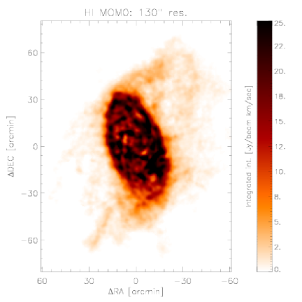
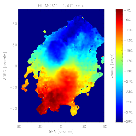
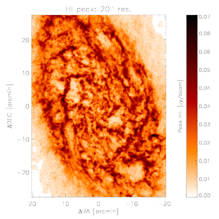
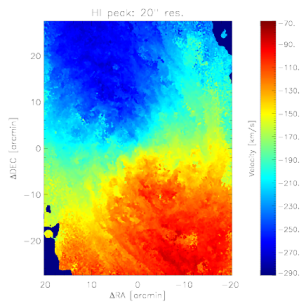
Figure 1: In the upper panels we show the integrated 21-cm line intensity and the intensity weighted mean velocity over the whole galaxy using the data at 130 arcsec resolution. In the lower panels we show the peak intensity and the velocity at peak maps using the VLA+GBT data at a resolution of 20 arcsec.

2.1 The molecular gas map

Rotational velocities in the innermost regions are complemented by the independent CO J=1-0 line dataset described by Corbelli (2003) at a spatial resolution of 45 arcsec (FCRAO survey). For the H₂ surface mass density radial scalelength we use the mean value between that determined by the FCRAO survey and that determined via the IRAM-30m CO J=2-1 line map of Gratier et al. (2010) (1.9 and 2.5 kpc respectively) i.e. we use the following expression to fit the molecular gas surface density:

$$\Sigma_{H_{2}}=10\times e^{-R/2.2}\qquad M_{\odot}\leavevmode\nobreak\ pc^{-2}$$ (1)

where $R$ is in kpc. The total gas mass in molecular form according to the above expression is 3.0$\times$10⁸ M_⊙, if integrated through the whole HI extent. This is in agreement with the molecular mass inferred by Corbelli (2003), Gratier et al. (2010) and more recently by Druard et al. (2014).

The atomic and molecular hydrogen gas surface densities have been multiplied by 1.33 to account for the helium mass when deriving the total gas mass surface density.

3 The stellar mass surface density

In this section we describe how the stellar mass surface density maps are derived: in §3.1 we present the method, then in §3.2 and 3.3 we describe the data and their processing and finally in §3.4 we present the results. The extension of the stellar mass distribution to distances larger than $\sim 5$ kpc is described in §3.5.

3.1 Method: from light to stellar mass

Maps of stellar mass surface densities can be derived from multiband optical imaging, as shown in the seminal work of Zibetti et al. (2009, ZCR09 hereafter), thanks to the relatively tight correlation existing between colors and the apparent stellar mass-to-light ratio ($M/L$, e.g. Bell & de Jong 2001). Here we implement an extension of the ZCR09 method, based on a fully bayesian approach, similar to the one adopted and validated by a number of works in the literature of the last decade (e.g. Kauffmann et al. 2003; Salim et al. 2005; Gallazzi et al. 2005; da Cunha et al. 2008; Gallazzi & Bell 2009). Our imaging dataset is composed of mosaic maps in the $B$, $V$ and $I$ bands from the Local Group Survey (Massey et al. 2006) and $g$ and $i$ bands from the Sloan Digital Sky Survey (York & et al. 2000, SDSS,). After processing the images as described in the following subsections, we perform a pixel by pixel stellar population analysis by comparing the measured magnitudes in the five bands with the corresponding magnitudes derived from a comprehensive model library of 150 000 synthetic spectral energy distributions (SED). Each model SED is computed with a stellar population synthesis (SPS) technique based on the most recent revision of the Bruzual & Charlot (2003, BC03, Charlot & Bruzual in prep.) simple stellar populations (SSPs), which use the “Padova 1994” stellar evolutionary library (see BC03 for details) and Chabrier (2003) stellar initial mass function (IMF). The SSPs are linearly combined according to a variety of star formation histories (SFH), parameterized and distributed as in Gallazzi et al. (2005, see their Sec. 2.3 for details), where random (in terms of time of occurrence, intensity and duration) bursts of star formation are superimposed onto continuous exponentially declining SFHs, with random initial time $t_{\mathrm{form}}$ and e-folding time scales $1/\gamma$. The metallicity of the stellar populations is fixed in each model along the SFH and is randomly chosen between 0.02 and 2.5 $Z_{\odot}$ from a uniform linear variate. Dust attenuation is also implemented following the simplified 2-component parameterization à la Charlot & Fall (2000) for the diffuse ISM and the stellar birth clouds: we adopt the same prescriptions as in da Cunha et al. (2008, see their sec. 2.1 for details). Each model is originally normalized so that the total mass in living stars and stellar remnants (white dwarfs, neutron stars and black holes) at the end of the SFH is 1 $M_{\odot}$. At each pixel, for each model $i$ we define the chi-square as follows:

$$\chi^{2}_{i}=\sum_{j=1}^{Nbands}{\frac{\left(m_{\mathrm{obs},j}-(m_{\mathrm{model},i,j}+ZP_{i})\right)^{2}}{\sigma_{j}^{2}}}$$ (2)

where $j$ runs over all bands used for the mass estimation, $m_{\mathrm{obs},j}$ is the observed magnitude of the pixel in the $j$-th band and $\sigma_{j}$ the corresponding error, $m_{\mathrm{model},i,j}$ is the magnitude of the model $i$ in the $j$-th band plus distance modulus, and $ZP_{i}$ is the zeropoint offset to apply to the model to match the observations. We then compute the $ZP_{i}$ that minimizes $\chi^{2}_{i}$. Since the models are originally normalized to 1 $\mathrm{M_{\odot}}$ in stars, the best-fitting stellar mass $M_{i}^{*}$ associated to the model $i$ is simply given by:

$$M_{i}^{*}=10^{(-0.4\leavevmode\nobreak\ ZP_{i})}\leavevmode\nobreak\ \mathrm{M_{\odot}}$$ (3)

To each model $i$ we further associate a likelihood

$$\mathcal{L}_{i}\propto\exp(-\chi_{i,\mathrm{min}}^{2}/2)$$ (4)

We can now build the unity-normalized probability distribution function (PDF) for the stellar mass at the given pixel: we consider the median-likelihood value (i.e. the value of stellar mass corresponding to the cumulative normalized PDF value of 0.5) as our fiducial estimate. The mass range between the 16-th and 84-th percentile of the PDF divided by 2 provides the error on the estimate. It is worth noting that the so-computed errors account for both photometric uncertainties and, importantly, also for intrinsic degeneracies between model colors and M/L.

The adoption of this bayesian median-likelihood estimator, instead of the simple conversion of light to mass via the M/L derived from a relation with one or two colors as done in ZCR09, allows to take full advantage of our multi-band dataset and reduce the impact of systematic effects in the individual bands (see next subsection).

We note that the BC03 revised models used here produce significantly higher stellar masses than those adopted in ZCR09, by some 0.1 dex. The main difference concerns the implementation of the TP-AGB evolutionary phase, which in the so-called “CB07” version predicts much higher luminosities than in the original BC03 models at fixed stellar mass. Recent works (e.g. Kriek et al. 2010; Conroy & Gunn 2010; Zibetti et al. 2013), however, have shown that the BC03 models are indeed closer to real galaxies than the CB07 ones and this motivates our choice.

3.2 The SDSS data

The Sloan Digital Sky Survey (York & et al. 2000, SDSS,) has covered M33 in several imaging scans, which must be properly background-subtracted and combined to obtain a suitable, science-ready map. From the SDSS we use only the $g$ and the $i$ band, which deliver the best signal-to-noise ratio out to the optical radius. We discard the $r$ band because of its contamination by H$\alpha$ line emission (see discussion in ZCR09). We reconstruct the separate scan stripes that cover M33 by stitching together the individual fields that we retrieved from the DR8 (Aihara & et al. 2011) data archive server. The SDSS pipeline automatically subtracts the background by fitting low order polynomials along each column in the scan direction. The process, however, is optimized to work with galaxies sizes of few arcminutes at most. In the case of M33, which is more than 1 degree across, the standard background subtraction algorithm fails by subtracting substantial fractions of the galaxy light. Therefore, we have added back the SDSS background and obtained the original scans, where only the flat-field correction has been applied.

For each column along the scan direction we determine the background as the best-fitting 5th degree Legendre polynomial, after masking out the elliptical region that roughly corresponds to the optical extent of M33 ($80\leavevmode\nobreak\ \mathrm{arcmin}\times 60\leavevmode\nobreak\ \mathrm{arcmin}$). This is achieved using the background task in the twodspec IRAF package, with a 2-pass sigma-clipping rejection at 3 $\sigma$. This procedure leaves large scale residuals in the backround regions, which we estimate at the level of $\approx 26.5$ mag arcsec^-2 in $g$ and $\approx 25.5-26$ mag arcsec^-2 in $i$ (r.m.s.). They are visible in the final mosaic maps as structure along the scan direction. We also checked that the extrapolation of the fit over the masked central area does not introduce spurious effects. In fact, the amplitude of the fitted polynomial along the scan direction never exceeds values corresponding to $\approx 24.5$ mag arcsec^-2 in the central regions, thus impacting their surface brightness by a few percent at most.

The scans are then astrometrically registered and combined in a wide-field mosaic using SWARP (Bertin et al. 2002). Bright Milky Way stars must be removed before surface photometry can be obtained. Stars are identified using SExtractor (Bertin & Arnouts 1996) on an unsharp-masked version of the mosaic. Bright young stellar association and compact star forming regions are manually removed, as our intent is to model the underlying (more massive) stellar disk, and such bright young features could bias the inferred M/L ratio downward. The original mosaic is then interpolated over the detected stars with a constant background value averaged around each star, using the IRAF task imedit. The size of the apertures for interpolation are optimized iteratively in order to minimize the residuals, and the brightest stars are edited manually for best results.

The edited SDSS mosaic is then smoothed with a gaussian of $\approx 100$ pc (25 arcseconds) FWHM in order to remove the stochastic fluctuations due to bright stars occupying the disk of M33, and finally resampled on a pixel scale of 8.3 arcsec/pix (i.e. $\approx 3$ pixels per resolution element). The $g$- and $i$-band surface brightness maps are finally corrected for the foreground MW extinction, by 0.138 and 0.071 mag respectively. Thanks to the massive smoothing and resampling, photon noise is largely negligible. The photometric errors are dominated by systematics in the photometric zero point and in the background subtraction. We conservatively estimate these sources of error as 0.05 mag for the zero-point (including also uncertainties related to the unknown variations of foreground Galactic extinction) and as 30% of the surface brightness for the background level uncertainty at $\mu_{g}=25$ and $\mu_{i}=24.5\leavevmode\nobreak\ \rm{magarcsec}^{-2}$ (which takes into account the aforementioned fluctuations in the residual background), respectively. The two contributions then are added in quadrature pixel by pixel. The zero-point uncertainty dominates in the inner and brighter parts of the galaxy, while the background uncertainty dominates at low surface brightness.

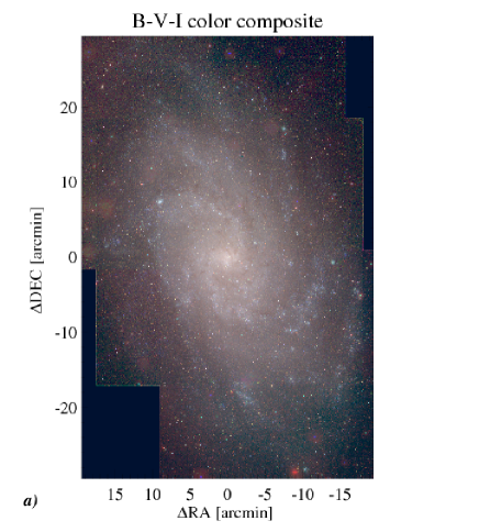
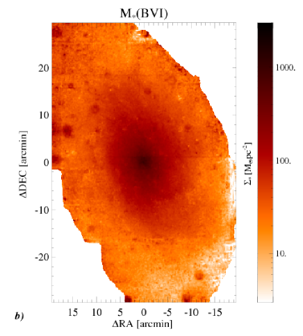
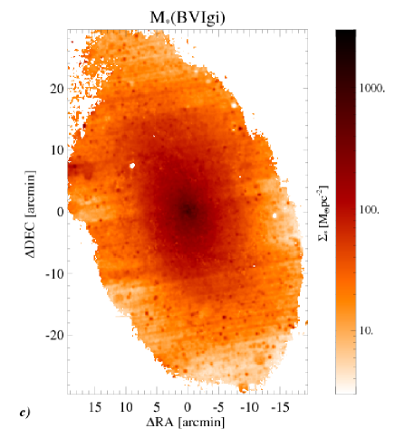
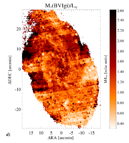
Figure 2: Panel a): The RGB color composite image of the B-V-I mosaics from the Massey et al. (2006) survey. Panel b): Stellar mass map derived from the median likelihood estimator (described in §3.1) based on LGS BVI bands. Panel c): Stellar mass map obtained from the bayesian median likelihood estimator, based on the full LGC and SDSS $BVIgi$ dataset. Panel d): The apparent stellar $M/L$ derived from the median likelihood stellar mass map based on LGS+SDSS $BVIgi$ bands and the observed LGS V-band surface brightness.

3.3 The Local Group Survey

The Local Group Survey (Massey et al. 2006) provides a set of deep wide-field images of M33 in the $UBVRI$ passbands (only $B$, $V$ and $I$ will be used to estimate the stellar mass in the following), together with a photometric catalog of 146,622 stars. Due to restrictions in the field of view, the galaxy was covered by acquiring three partially overlapping fields (C,N,S) in each band, a total of 15 images. All these images, together with those secured in narrow bands, are publicly accessible but no photometric calibration is provided due to the composite nature of the mosaicing CCD detector. In order to calibrate the images, we select from the photometric catalog a set of stars brighter than $V=16.00$: 195 stars in the C field, 114 in the N, and 76 in the S. First we measure the size of the PSF in the images and then degraded all of them to match the seeing of the worst one (the N field in the $I$ band with a gaussian $\sigma=0.35$ arcsec). Next, we perform multi-aperture photometry of the selected stars and derive the calibration by comparing fluxes with the values reported in the catalog. Note, the multi-aperture photometry also provides the background offsets between the 3 different fields in each band. After readjusting the background and the scale of the N and S fields to C, the fields are combined to produce an image of the entire galaxy which is later sky subtracted by using the most external regions. After registering the positions to the V-band reference, the images are again calibrated with the same procedure outlined above but including color terms. A full resolution RGB color composite image of the $B-V-I$ bands is shown in Fig. 2, top left panel.

The $B$, $V$ and $I$ band calibrated maps are then edited, degraded in resolution and resampled to match the SDSS images described in the previous subsection. From the calibration procedure of these final maps, again by comparison with the photometry of the stars with $V\leq 16.00$ in the Local Group Survey catalog, we determine uncertainties in the zero-point of 0.02. 0.10, and 0.18 mag in the $B$, $V$ and $I$ band, respectively. These final maps are also used for determining the background subtraction. 20 fields containing no stars, each 20x20 arcsec in extent, were selected in the far NE and SW regions at the borders of the image; these fields show minimal emission in all three bands. In each bandpass, we assume the background to be the mean of the 20 median values, and the background uncertainty to be the $1\sigma$ of the sample (not of the mean); this uncertainty amounts to 30% of the surface brightness at $\mu_{B}=25.0,\mu_{V}=24.3,\mu_{I}=23.5$, respectively.

3.4 Stellar mass map(s)

The left bottom panel of Fig. 2 shows the map of stellar mass derived from the pixel-by-pixel analysis described in §3.1, using both the $BVI$ maps from LGS and the $gi$ maps from SDSS. The smoothness and azimuthal symmetry of the map is remarkable, although, especially at low surface density values, one can clearly see background residuals appearing as large scale “spot” fluctuations (coming from the LGS maps) and fluctuations along stripes (coming from the SDSS scans). Random errors on this map (as derived from the inter-percentile range of the PDF described in Sec. 3.1) range from 0.06 to 0.1 dex (approximately 15 to 25%), including the contribution of both photometric uncertainties and intrinsic model degeneracies between colors and M/L, but not systematics (see end of this section).

In the bottom right panel of Fig. 2 we display the map of the ratio between the estimated stellar mass and the V-band surface brightness (as measured) in solar units. This figure makes it obvious that a simple rescaling of the surface brightness by a constant mass-to-light ratio (as is usually done in the dynamical analysis) is a very crude approximation to the real stellar mass distribution. In particular, the M/L gradients apparent from this map substantially affect the slope of the mass profile, as discussed more in detail in Section 6.

Figure 2, with its many apparent artefacts, also highlights the limits of our photometry, mainly due to the difficulties of obtaining an accurate background subtraction in such a large-scale mosaic. On the other hand, the redundancy of our dataset in terms of wavelength coverage reveals its importance to limit the impact of systematic effects when we compare the mass surface density obtained from the full $BVIgi$ dataset (bottom left panel of Fig. 2) to that obtained from the LGS dataset alone (upper right panel). In particular, the comparison shows that i) the anomalously high surface density that appear in the outskirts of the map based on LGS alone are corrected by including also SDSS imaging, most likely thanks to a more accurate background subtraction in the SDSS; ii) the North-South asymmetry evident in the LGS map is also corrected by a more stable and accurate zero-point determination in the SDSS. Moreover, we note that the stripe structure introduced by the background subtraction in the SDSS images is partly removed by the inclusion of LGS images.

Despite some differences in the overall normalization, the mass surface density variations in the two maps are consistent. The stellar mass map derived from the full dataset (LGS+SDSS) will be our reference mass distribution but we shall carry out the dynamical analysis using both maps, limiting the usage of the mass map from the LGS dataset to R$<4$ kpc. Considering the uncertainties derived from our bayesian marginalization approach (thus combining model degeneracies and random photometric errors) and comparing the two mass maps obtained with the two photometric datasets, we estimate a typical stellar mass uncertainty of $\sim 30$% (0.11 dex) out to $\mu_{B}=25$, which we apply to the dynamical analysis. We stress once again that the uncertainties derived from the interpercentile range of the PDF over a large and comprehensive library of model star-formation histories, metallicity and dust distributions, de facto realistically include the contribution of the systematic uncertainties related to the choice of models. This is one of the key advantage in using this approach with respect to other maximum-likelihood fitting algorithms, either parametric or non-parametric.

The only possible systematic uncertainties that are not included in the error budget are the ones related to the IMF, which is kept fixed in all models (to the Chabrier IMF), and those related to the basic ingredients of stellar population synthesis, i.e. the base SSPs. One can of course include models with different IMFs in the library, but broad band optical colors are essentially insensitive to it, hence they do not provide any constraint in that respect. Possible different IMFs should thus be treated as an extra freedom in the stellar mass normalization. Testing different SSPs is clearly out of the scope of this paper. However, it is worth mentioning that after many years of debate about the role of TP-AGB stars in stellar populations, the community is reaching a broad consensus on their limited role (e.g. Kriek et al. 2010; Conroy & Gunn 2010; Zibetti et al. 2013), thus leaving little freedom on the intrinsic M/L of simple stellar populations at fixed SED. Therefore this contribution to the mass error budget appears negligible in comparison with the variations induced by different star formation histories, metallicity and dust distributions, already accounted for by our method of error estimates.

3.5 The outermost stellar disk

As pointed out by several surveys (e.g. McConnachie et al. 2010), the stellar disk of M33 extends out to the edge of the HI disk following a similar warped structure. To account for this fainter but extended disk we first extrapolate the stellar mass surface density of the inner stellar map outward to 10 kpc, using the radial scalelength inferred by the 3.6 $\mu$m map (Verley et al. 2007, 2009). This scalelength, 1.8$\pm 0.1$ kpc, is consistent with that inferred in our stellar surface density maps beyond R$\sim$ 2 kpc. Stellar counts from deep observations of several fields further out, in the outer disk of M33, have been carried out by Grossi et al. (2011) using the Subaru telescope. The typical face-on radial scalelength of the stellar mass density in the outer disk inferred from these observations is 25 arcmin ($\sim$6 kpc), much larger than that of the brighter inner disk and very similar to the HI scalelength in the same region. We shall use this radial scaling to extrapolate exponentially the stellar surface density further out and truncate the profile with a sharp fall off beyond 22 kpc.

4 The rotation curve

In this Section we outline the derivation of the rotation curve of M33 starting from an analysis of the spatial orientation of the disk.

4.1 The warped disk

To make a dynamical mass model of a disk galaxy it is necessary to reconstruct the three-dimensional velocity field from the velocities observed along the line of sight. If velocities are circular and confined to a disk one needs to establish the disk orientation i.e. the position angle of the major axis (PA), and the inclination ($i$) of the disk with respect to the line of sight. If the disk exhibits a warp these parameters vary with galactocentric radius. This is often the case for gaseous disks which extend outside the optical radius and which show different orientations than the inner ones. Tilted ring model are considered to infer the rotation curve of warped galactic disks. Corbelli & Schneider (1997) have fitted a tilted-ring model to the 21-cm line data over the full extent of the M33-HI disk. However the disk was not fully sampled by the data since the observations (carried out with the Arecibo flat feed, FWHM=3.9 arcmin) only sampled the disk over an hexagonal grid with 4.5 arcmin spacing. To determine the disk orientation using the new 21-cm all-disk survey described in this paper, we follow a tilted ring model procedure which departs from the usual schemes and which has been used by Corbelli & Schneider (1997) and later implemented by Józsa et al. (2007) (TiRiFiC, a Tilted Ring Fitting Code, available to the public). A set of free rings is considered, each ring being characterized by its radius $R$ and by 7 additional parameters: the HI surface density $S_{HI}$, the circular velocity $V_{c}$, the inclination $i$ and the position angle PA, the systemic velocity $V_{sys}$ and the position and velocity shifts of the orbital centers with respect to the galaxy center ($\Delta x_{c},\Delta y_{c}$). Importantly, rather than fitting the moments of the flux distribution, we infer the best fitting parameters by comparing the synthetic spectra of the tilted ring model to the full spectral database, as explained in details in Appendix A. In Appendix A we described also the two minimization methods used, the ’shape’ and ’v-mean’ methods, which give consistent results for the M33 ring inclinations and position angles.

We display the best fitting values of $i$ and PA in Figure 3 with their relative uncertainties. As we can see from Figure 3 the orientation of the outermost rings has high uncertainties. This is especially remarkable when using the ”shape” method and hence we fix the outermost ring parameters to be equal to those of second-last ring for deconvolving the data. The intermediate regions solutions appear to be more robust. In the next subsection the best fitting values of systemic velocity shifts and ring center displacements (shown in Appendix A) will be used together with the rings orientation angles, $i$ and PA, to derive rotational velocities V_r and the face-on surface brightness $\Sigma_{HI}$ from the data at high and low resolution. Notice that the values of V_r and $\Sigma_{HI}$ we infer are consistent with the value of the free parameters $V_{c}$ and $S_{HI}$ of the adopted ring model but will be sampled at a higher resolution along the radial direction.

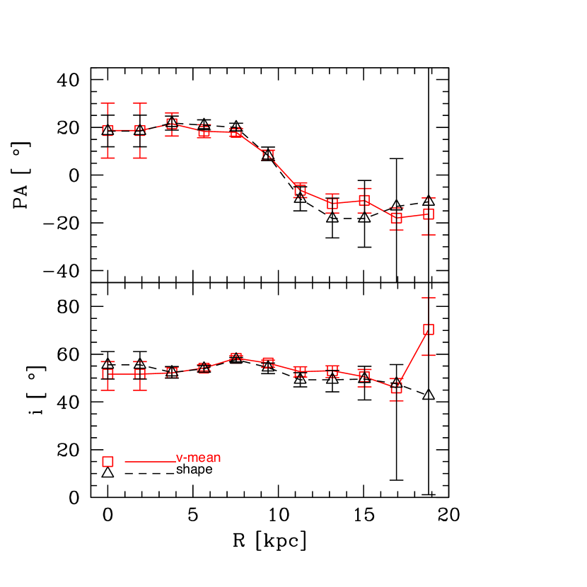
Figure 3: The inclination and position angle of the 11 free tilted rings used for deconvolving the 21-cm data. The open triangles (in black in the on-line version), connected by a dashed line, shows the value using the shape minimization method, the open squares (in red in the on-line version), connected by a continuous line, are relative to the v-mean minimization method (see Appendix A for details). The uncertainties are computed by varying one parameter of one free ring at a time around the minimal solution until the $\chi^{2}$ of the tilted ring model increases by 2$\%$ .

4.2 The 21-cm velocity indicators

To derive the rotation curve we use the 21-cm datacube at a spatial resolution of 20 and 130 arcsec. Emission in the high spatial resolution dataset is visible only out to R=10 kpc while in the lower resolution dataset the HI is clearly visible over a much extended area. To trace the disk rotation we consider both the peak and the flux weighted mean velocities (moment-1) along the line of sight of the 21-cm line emission at the original spectral resolution. The velocity at the peak of the line is in general a better indicator of the disk rotation than the mean velocity when the signal-to-noise is high and the rotation curve is rising (e.g. de Blok et al. 2008) and we will use this velocity indicator inside the optical disk. In the outer disk, where the signal-to-noise is lower and the rotation curve is flatter we use instead the flux weighted mean velocities (as well shall see, the curves traced by the two velocity indicators in this regions are quite consistent).

The rotation curve of M33 is extracted from the adopted line-of-sight velocity indicator using as a deconvolution model the best-fit disk geometrical parameters (derived via the shape and v-mean methods, described in Appendix A, which we shall call model-shape and model-mean). The model-shape and model-mean parameters are shown in Figure 18 and in Figure 3. If 21-cm emission is present in some area located at larger radii than the outermost free ring we deconvolve the observed velocities assuming a galaxy disk orientation as the outermost free ring.

When using the mean instead of the peak velocity, the same deconvolution model results in a rotation curve with lower rotational velocities. In the optical disk the difference between the rotation curve traced by the peak or the mean velocities can be as high as 10 km s^-1 but the scatter between the results relative to the two deconvolution models is small (it is always less than $2$ km s^-1 and for most bins less than $1$ km s^-1). Further out there are no systematic differences between the curve traced by the peak and the mean velocity but the outermost part is very sensitive to the orientation parameters adopted. These parameters are not tightly constrained in the outermost regions due to the partial coverage of the modeled rings with detectable 21-cm emission and to some multiple component spectra. Here it will be important to consider the deconvolution model uncertainties in the rotation curve.

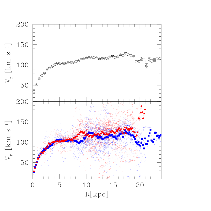
Figure 4: The bottom panel shows with small dots the rotational velocities for each pixel in the peak map (red dots for the southern half and blue dots for the northern half in the on-line version) and with large symbols the average values in each radial bin. The model-shape has been used to deconvolve the data. Triangles (red in the on-line version) are for the southern half while squares (blue in the on-line version) are for the northern half. The top panel shows the average rotation curve for peak velocities. Bins are 2 arcmin wide in the radial direction.

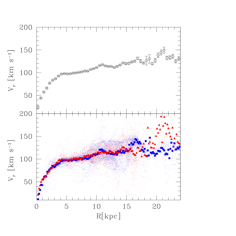
Figure 5: The bottom panel shows with small dots the rotational velocities for each pixel in the first moment-1 map and with large symbols the average values in each rings (Red symbols are for the southern half and blue symbols for the northern half in the on-line version). The model-mean has been used to deconvolve the data. Triangles are for the southern half while squares are for the northern half. The top panel shows the average rotation curve for moment-1 (mean) velocities. Bins are 2 arcmin wide in the radial direction.

In Figure 4 and in Figure 5 we show the rotation curve from the peak and the mean velocities, the first one obtained from the tilted-ring model-shape and the second one from model-mean. For the outer disk we use the low resolution dataset with 2 arcmin radial bins (0.5 kpc wide). For the inner disk the high resolution data are binned in 40 arcsec radial bins (163 pc wide). In Figure 6 we show the curve traced by the peak velocities after averaging the rotational velocities relative to the deconvolution model-shape and deconvolution model-mean. In the same Figure the filled dots show the curve from the low resolution dataset which matches perfectly the high resolution curve. To not overweight the inner rotation curve in the dynamical analysis we will use the low resolution 21-cm dataset in addition to the velocities of the CO-J=1-0 line peaks (black stars in Figure 6). The average values of PA and $i$ between deconvolution model-shape and model-mean are used to trace the rotation curve with CO J=1-0 line. These deconvolution parameters have been used also to trace the inner curve with the moment-1 velocities, which is shown for comparison in Figure 6 (open square symbols). There is not much difference between the rotational velocities retrieved from model-shape or model-mean in the inner region but the moment-1 velocities give clearly lower rotation curve than the peak velocities.

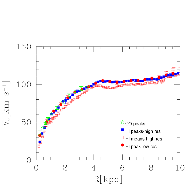
Figure 6: The inner rotation curve as traced by the peak velocities at high resolution (filled squares in blue in the on-line version), and at low resolution (filled dots in red in the on-line version). The CO data are shown with star symbols (in green in the on-line version). The open square symbols (in red in the on-line version) are for rotational velocities as traced by the moment-1 map. For each curve the weighted mean velocities between that relative to deconvolution model-shape and model-mean are used.

4.3 Rotation curve: a comparative approach

In this subsection we compare the rotation curve derived through our technique of fitting the 21-cm line emission (the datacube) with a tilted ring model, to those resulting from other type of approaches and methods. These complementary approaches are useful to strengthen the robustness of the rotation curve and to better define the uncertainties. We consider two additional methods devised for deriving galaxy rotation curves from two-dimensional moment-maps. The first one is the standard least-square fitting technique developed by Begeman (1987) as implemented in the ROTCUR task within the NEMO software package of analysis (Teuben 1995). The other method is based on the harmonic decomposition of the velocity field along ellipses and we use for this purpose the software KINEMETRY developed and provided by Krajnović et al. (2006). Both methods work on 2D momentum maps i.e. on one velocity per pixel, and minimize the free parameters of one ring at a time, without accounting for possible overlaps of ring pieces in the beam. We run ROTCUR in two steps: at first we let the ring centers and V_sys vary. The orbital center shifts are larger in the outermost regions and roughly in the direction of M31, as found by Corbelli & Schneider (1997), and are shown in Figure 8. In the second iteration we fix the ring centers and V_sys to the average values found in the first iteration, x_c=-33 arcsec y_c=105 arcsec V_sys=-178 km s^-1. We run a second iteration because by fixing the orbital centers the routines converge further out, at radii as large as R=23.5 kpc. In this second attempt we run ROTCUR with 51 free rings, uniform weight, excluding data within a 20^∘ around the minor axis. The resulting PA and $i$ are shown in the top panel of Figure 7. With the KINEMETRY routines we fit with a smaller number of free rings, 10, and convergence is achieved over a smaller radial range, out to R=17.5 kpc. The higher order terms of the harmonic decomposition are useful tools if one is looking for non-circular motion in the disk. In the bottom panel of Figure 7 we show the usual PA and $i$ but in addition we plot the coefficient $k_{5}$ in Figure 8. This is an higher order term which represents deviations from simple rotation due to a separate kinematic component like radial infall or non-circular motion. Its amplitude is negligible in the optical disk but it is as high as 7 km s^-1 in the outer disk. If the anomalous velocities are in the radial direction this gas can be fueling star formation in the inner disk.

Figure 7: The tilted ring position angles and inclinations are shown with open square symbols and filled dot symbols respectively for the ROTCUR and KINEMETRY fitting routines.

Figure 8: Some of the tilted ring parameters fitted by the routines ROTCUR and KINEMETRY. The top panel shows the term k5, which is an higher order term in the KINEMETRY outputs. In the bottom panel we show the shifts of the systemic velocity and in the middle panel the orbital center shifts along the y-axis in the South-North direction (filled square symbols) and along the x-axis oriented from East-to-West (open square symbols).

The two rotation curves obtained with the NEMO and KINEMETRY routines are very similar to the one derived from the deconvolution model-shape and -mean inside the optical disk, but there are some differences in the resulting warp orientation and hence in the outer rotation curve. This can be seen in Figure 9. There are very marginal differences between the rotation curves of the inner region relative to different deconvolution models. Beyond 15 kpc instead there are significant differences which we take into account.

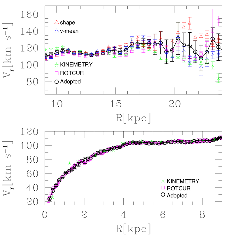
Figure 9: The open black circles show the adopted rotation curve for the inner regions (bottom panel) using the peak velocities and for the outer regions (top panel) using the first moments. The dispersions take into account variation of V_r between different deconvolution models, the 2$\%$ variations around the minimum $\chi^{2}$ and the standard deviation of the mean velocity in each bin. In both panels the open square and asterix symbols (in magenta and green in the on-line version) show V_r according to the ROTCUR and KINEMETRY deconvolution model respectively. In the top panel the open triangles are for the first moment velocities deconvolved according to model-shape and model-mean (in red and blue colors respectively in the on-line version).

4.4 The adopted rotation curve and its uncertanties

For the final rotation curve of M33 we use the following recipe. Inside the optical disk we use representative 21-cm peak circular velocities computed as the weighted mean of velocities originating from our two deconvolution choices (model-shape and model-mean). To these we append the CO dataset. Beyond 9 kpc, in each radial bin we use the weighted mean circular velocity computed by averaging the moment-1 velocities resulting from: (1) the deconvolution model-shape, (2) the deconvolution model-mean, (3) the package KINEMETRY and (4) the task ROTCUR in NEMO package.

The rotation curve uncertainties take into account not only the standard deviations around the mean of the 2 or 4 velocities averaged, but also the data dispersion in each radial bin (see data in bottom panels of Fig 4 and 5) and the uncertainties relative to deconvolution models ($\Delta V_{r}$ corresponding to 2$\%$ $\chi^{2}$ variations of the tilted ring model-shape and -mean through PA and $i$ displacements).

To the final rotation curve we apply the small finite disk thickness corrections, described in Appendix B.

5 The surface density of the baryons

In this Section we use the radial profile of the stellar mass surface density from the $BVIgi$ maps, together with the gaseous surface density, to compute the total baryonic face-on surface mass density of M33 and the stellar mass-to-light ratio. The surface density of stars perpendicular to the disk is shown in Figure 10: it drops by more than 3 orders of magnitudes from the center to the outskirts of the M33 disk. The total stellar mass according to the $BVIgi$-mass map extrapolated to the outer disk is 4.9 10⁹ M_⊙ (5.5 10⁹ M_⊙ for the BVI map) of which about 12 $\%$ resides in the outer disk. At the edge of the optical disk Barker et al. (2011) find a surface density of stars $\sim$1.7 M_⊙/pc² for a Chabrier IMF down to 0.1 solar masses assuming the inclination of our tilted ring model. This is consistent to what our modeled radial stellar distribution predicts at 9 kpc: 1.7$\pm 0.5$ M_⊙/pc². The outermost field (S2) of Barker et al. (2011) has been placed outside the warped outer disk and hence traces only a possible stellar halo.

Using the best fitting tilted ring model we derive the radial distribution of neutral atomic gas, perpendicular to the galactic plane, in the optically thin approximation. This is shown in Figure 10. The total HI mass computed by integrating the surface density distribution in Figure 10 out to 23 kpc is about 20$\%$ higher than the true HI mass of the galaxy, which is 1.53$\times 10^{9}$ M_⊙. This is because we average the flux of all pixels with non-zero flux in each ring and the HI emission in the outermost rings does not cover the whole ring surface. We do this because it is likely that undetected pixels at 21-cm are not empty areas but host ionized gas. In fact, a sharp HI edge has been detected in this galaxy as the gas column density approaches 2$\times$ 10¹⁹ cm^-2 and interpreted as an HI–¿HII transition (Corbelli & Salpeter 1993). Considering the irregular outer HI contours of M33 as being due to ionization effects, the outermost part of the atomic radial profile is in reality an HI+HII profile since there is HII where HI lacks at a similar column density. This assumption has a negligible effect on the dynamical analysis of the rotation curve. The continuous line in Figure 10 is the log of the function used to compute the dynamical contribution of the hydrogen mass to the rotation curve. The total baryonic surface density is computed adding to the hydrogen gas the stellar mass surface density, the molecular and the helium mass surface density (as given in Section 2.2). Stars dominate the potential in the star-forming disk ($R<7$ kpc), beyond this radius stars and gas give a similar contribution to the baryonic mass surface density and decline radially in the outer disk with a similar scalelength.

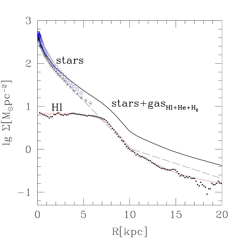
Figure 10: The HI surface density perpendicular to the galactic plane of M33 (small filled triangles) and the function which fits the data (continuous line, red in the on-line version) after the 21-cm line intensity has been deconvolved according to tilted ring model-shape. Asterix symbols indicate the stellar mass surface density using the $BVIgi$ stellar surface density map. The dashed line is the fit to the stellar surface density and the extrapolation to larger radii. Open squares (in blue in the on-line version) show for comparison the surface density using the BVI mass map. The heavy weighted line is the total baryonic surface density, the sum of atomic and molecular hydrogen, helium and stellar mass surface density.

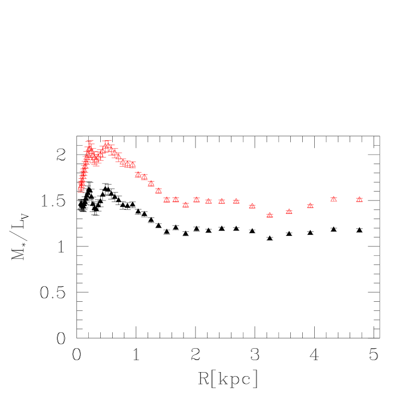
Figure 11: The mass-to-light ratio as a function of galactocentric radius according to the $BVIgi$ stellar surface density map (filled triangles, in black in the on-line version). This is computed by averaging the stellar mass map and the V-band surface brightness along ellipses corresponding to the tilted ring model. We then compute M_∗/L_V as the ratio between these two quantities in units of M_⊙/L_⊙. We show for comparison the same ratio relative to the BVI stellar surface density map (open triangles, in red in the on-line version). The error bars are the standard deviations relative to azimuthal averages and do not take into account uncertainties in the mass determination.

The mass-to-light ratio as a function of galactocentric radius is computed by averaging the $BVIgi$ stellar surface density map and the V-band surface brightness along ellipses corresponding to the tilted ring model. The filled triangles in Figure 11 show the ratio between these quantities, M_∗/L_V, in units of M_⊙/L_⊙. We show for comparison the same ratio relative to the BVI stellar surface density map (open triangles). Despite some differences in the two maps, the shape of the azimuthally averaged radial profiles of the mass surface density are consistent. Only in the innermost 1 kpc there is some difference in the radial decline. The error bars are the standard deviations relative to azimuthal averages and do not take into account uncertainties in the mass determination. We clearly see radial variations of the mass-to light ratio, especially in the innermost 1.5 kpc relative to areas at larger galactocentric radii. This is an effect of the inside-out disk formation and evolution which adds to more localized variations present in the map such as in arm-interarm contrast.

Average values or radial dependencies of the mass-to-light ratios, shown in Figure 11, can be compared with those derived previously using different methods. The dynamical analysis of planetary nebulae in M33 (Ciardullo et al. 2004) gives a mass-to-light ratios which increase radially, being 0.2 M${}_{\odot}/L_{V}\odot$ at R=2 kpc and 0.8 M${}_{\odot}/L_{V}\odot$ at 5 kpc. However, this result is based on the assumption of radially constant vertical scaleheight and of a much longer radial scalelength of the stellar surface density than suggested by near-infrared photometry. These assumptions imply also a strong radial decrease of the velocity dispersion if the disk is close to marginal stability, in disagreement with what is observed for the atomic gas. A more recent revised model for the marginally stable disk of M33 (Saburova & Zasov 2012)implies a flatter mass-to-light ratio, of order 2 M${}_{\odot}/L_{V}\odot$ in closer agreement with what we find. An increase of the mass-to-light ratio in the central regions of M33 and a stellar mass surface density with very similar values to what we show in Figure 10 has been found by Williams et al. (2009) using resolved stellar photometry and modeling of the color-magnitude diagrams.

The former M33 rotation curve (Corbelli 2003) was best fitted using CDM dark halo models by assuming an average stellar mass-to-light ratio in the range 0.5-0.9 M${}_{\odot}/L_{V}\odot$, a somewhat smaller value that derived here. However Corbelli (2003) considered an additional bulge component whose presence has not been supported by subsequent analysis Corbelli & Walterbos (2007). From the stellar mass model presented here it seems more likely that the M33 disk has larger mass-to-light ratio in the innermost 1.5 kpc rather than a genuine bulge. As it will be shown in the next Section, a radially varying mass-to-light ratio without a bulge component gives a similar CDM halo model for M33. On the other hand the constraints on the stellar mass-to-light ratio given by our mass map will be hard to reconcile with some dark halo model.

6 Tracing dark matter via dynamical analysis of the rotation curve

The dynamical analysis of a high resolution rotation curve, such as that presented in this paper for M33, together with detailed maps of the baryonic mass components, provides a unique test for the dark matter halo density and theoretical models of structure formation and evolution. In this Section we shall consider a spherical halo with a dark matter density profile as originally derived by Navarro et al. (1996, 1997) (hereafter NFW) for galaxies forming in a Cold Dark Matter scenario. We consider also the Burkert dark matter density profile (or core model) (Burkert 1995) since this successfully fitted the rotation curve of dark matter dominated dwarf galaxies (e.g. Gentile et al. 2007, and references therein). Both models describe the dark matter halo density profile using two parameters which we determine through the best fit to the rotation curve. Our last attempt will be to fit the rotation curve using MOdified Newtonian Dynamics (MOND).

We perform a dynamical analysis of the rotation curve in the radial range: $0.4\leq R\leq 23$ kpc. For the gas and the stellar surface density distribution we consider the azimuthal averages shown in Figure  10. Given the 30$\%$ uncertainty for the stellar mass surface densities we shall consider total M_∗ in the following intervals: $9.57\leq$ log M${}_{*}\leq 9.81$ M_⊙ when using the $BVIgi$ mass map and $9.62\leq$ log M${}_{*}\leq 9.86$ M_⊙ when using the BVI mass map. The vertically uniform gaseous disk is assumed with half thickness of 0.5 kpc and a flaring disk is considered for the stellar disk with a half thickness of 100 pc at the center, reaching 1 kpc at the outer disk edge. The contribution of the disk mass components to the rotation curve is computed according to Casertano (1983), who generalizes the formula for the radial force to thick disks. We use the reduced chi-square statistic, $\chi^{2}$, to judge the goodness of a model fit.

6.1 Collisionless dark matter: a comparison with LCDM simulations

The NFW density profile is usually written as:

$$\rho(R)={\rho_{NFW}\over{R\over R_{NFW}}\Bigl{(}1+{R\over R_{NFW}}\Bigr{)}^{2}}$$ (5)

where $\rho_{NFW}$ and $R_{NFW}$ are the characteristic density and scale radius, respectively. Numerical simulations of galaxy formation find a correlation between $\rho_{NFW}$ and $R_{NFW}$ which depends on the cosmological model (e.g. Navarro et al. 1997; Avila-Reese et al. 2001; Eke et al. 2001; Bullock et al. 2001). Often this correlation is expressed using the concentration parameter $C\equiv R_{vir}/R_{NFW}$ and $M_{h}$ or $V_{h}$. $R_{vir}$ is the radius of a sphere containing a mean density $\Delta$ times the cosmological critical density. $\Delta$ varies between 93 and 97 depending upon the adopted cosmology (Macciò et al. 2008). This corresponds to a mean halo overdensity of about 360 with respect to the cosmic matter density at z=0. $V_{h}$ and $M_{h}$ are the characteristic velocity and mass at $R_{vir}$. In this paper we compare our best fitted parameters C and M_h with the results of N-body simulations in a flat $\Lambda$CDM cosmology using relaxed halos for WMAP5 cosmological parameters (Macciò et al. 2008). In particular, we shall refer to the relation between the mean concentration and virial mass of dark halos resulting from the numerical simulation of Macciò et al. (2008) whose dispersion is $\pm 0.11$ around the mean of log$C$. The resulting C–M_h relation is similar to that found by Macciò et al. (2007) and more recently by Prada et al. (2012).

We now fit the M33 rotation curve using as free parameters the dark halo concentration, $C$, and mass, M_h. We fix the stellar mass surface density distribution to that given by our mass maps extrapolated outwards, as explained in the previous section. We allow a scaling factor to account for the model and data uncertainties i.e. we consider total stellar masses log M${}_{*}/M_{\odot}=9.69\pm 0.12$ and log M${}_{*}/M_{\odot}=9.74\pm 0.12$ for the $BVIgi$ and BVI mass distributions, respectively. The best fits using the two mass maps are very similar as shown in the bottom panel of Figure 12. The reduced $\chi^{2}$ are 0.96 and 1.08 for the BVI and $BVIgi$ stellar mass distributions respectively with log M${}_{*}/M_{\odot}$=9.8, close to the upper limit of our considered range. The dark matter halo for the best fits has concentration C=6.7 and mass M_h=5$\times 10^{11}$ h^-1 M_⊙. A close inspection of the 1,2,3-$\sigma$ confidence areas in the log C –log M${}_{h}/h^{-1}$ plane and in the log M_∗–log M${}_{h}/h^{-1}$ plane, shown in Figure 13, reveals that indeed there is still some degeneracy in the C–M_h plane: a lighter stellar disk can provide good fits to the rotation curve if a less massive dark halo with a higher concentration is in place. Confidence areas are traced in Figure 13 only for the allowed stellar mass range. In Figure 13 we also show the most likely value of the stellar mass computed by the synthesis models (dot-dashed line in the upper panels) and the log C–log M${}_{h}/h^{-1}$ relation as from $\Lambda$CDM numerical simulations (continuous line Macciò et al. 2008) and its dispersion around the mean (dashed lines). The values of C and M_h suggested by the dynamical analysis of the M33 rotation curve are in good agreement with the $\Lambda$CDM predictions.

We now compute the most likely values of the free parameters, C, M_h, and M_∗ by considering the composite probability of 3 events: $i)$ the dynamical fit to the rotation curve, $ii)$ the stellar mass determined via synthesis models, $iii)$ the log C–log M${}_{h}/h^{-1}$ relation found by numerical simulations of structure formation in a $\Lambda$CDM cosmology. The composite probability gives smaller confidence areas in the free parameter space, shown in Figure 14, which are very similar for the two mass maps. The model with the highest probability has the following parameters for the $BVIgi$ mass map and $h=0.72$: M${}_{*}=4.9^{+0.5}_{-0.7}\times 10^{9}\leavevmode\nobreak\ M_{\odot}$, M${}_{h}=3.9^{+1.0}_{-0.6}\times 10^{11}\leavevmode\nobreak\ M_{\odot}$, C=$10\pm 1$, and the fit to the rotation curve, shown in the upper panel of Figure 12, has a $\chi^{2}=1.3$. For the BVI map we get M${}_{*}=4.8^{+0.4}_{-0.4}\times 10^{9}\leavevmode\nobreak\ M_{\odot}$, M${}_{h}=4.6^{+0.7}_{-0.6}\times 10^{11}\leavevmode\nobreak\ M_{\odot}$, C=$9\pm 1$ with a $\chi^{2}=1.1$ for the dynamical fit shown in the upper panel of Figure 12. Given the marginal differences in the two sets of free parameters we can summarize the best fit $\Lambda$CDM dark halo model for M33 as follows:

$$M_{h}=(4.3{\pm 1.0})\times 10^{11}\leavevmode\nobreak\ M_{\odot}\qquad C=9.5\pm 1.5$$ (6)

and the total stellar disk mass estimate is M${}_{*}=(4.8{\pm 0.6})\times 10^{9}$ M_⊙. The resulting dynamical model implies that the contribution of the dark matter density to the gravitational potential is never negligible, although it becomes dominant outside the star forming disk (R$>7$ kpc) where the stellar and gaseous disk gives a small, but similar contribution to the rotation curve.

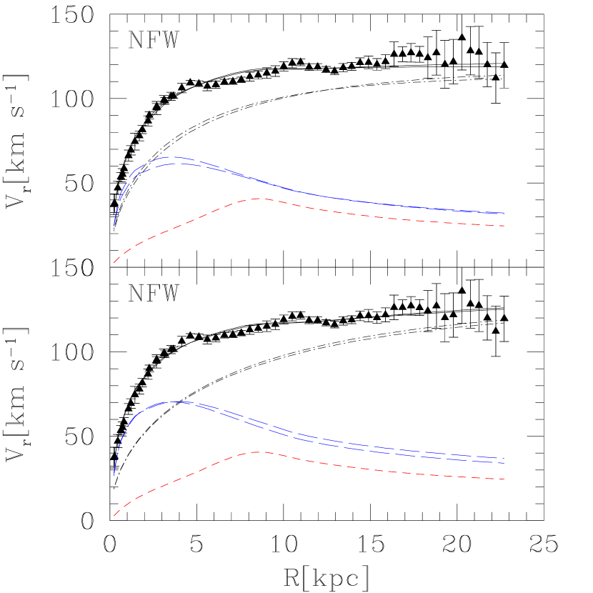
Figure 12: The rotation curve of M33 (filled triangles) and best fitting dynamical models (solid line) for NFW dark matter halo profiles (dot-dashed line). The small and large dashed lines (red and blue in the on-line version) show respectively the gas and stellar disk contributions to the rotation curve. In the bottom panel the highest stellar contribution and lowest dark halo curve are for the best fitting dynamical model using the $BVIgi$ mass map, the other curves are for the BVI mass map. The top panel shows the most likely dynamical models for the two mass maps when the likelihood of the dynamical fit is combined with that of the stellar mass surface density and of the C–M_h relation resulting from simulations of structure formation in a $\Lambda$CDM cosmology.

Figure 13: The 68.3$\%$ (darker regions, blue in the on-line version), 95.4$\%$ (magenta) and 99.7$\%$ (lighter regions, cyan) confidence areas in the log C–log M${}_{h}/h^{-1}$ plane and in the M_∗–M${}_{h}/h^{-1}$ plane for the dynamical fit to the rotation curve using a NFW dark matter halo profile. The mass distribution is that given by the $BVIgi$ colors for the areas shown in $(a)$ and $(b)$, and by the BVI colors for the areas in $(c)$ and $(d)$. In panels $(a)$ and $(c)$ we show the C–M_h relation (solid line) and its dispersion (dashed line) for $\Lambda$CDM cosmology. In panel $(b)$ and $(d)$ the dash-dot line indicates the most likely stellar mass according the synthesis models which rely on the colors following the panel labels.

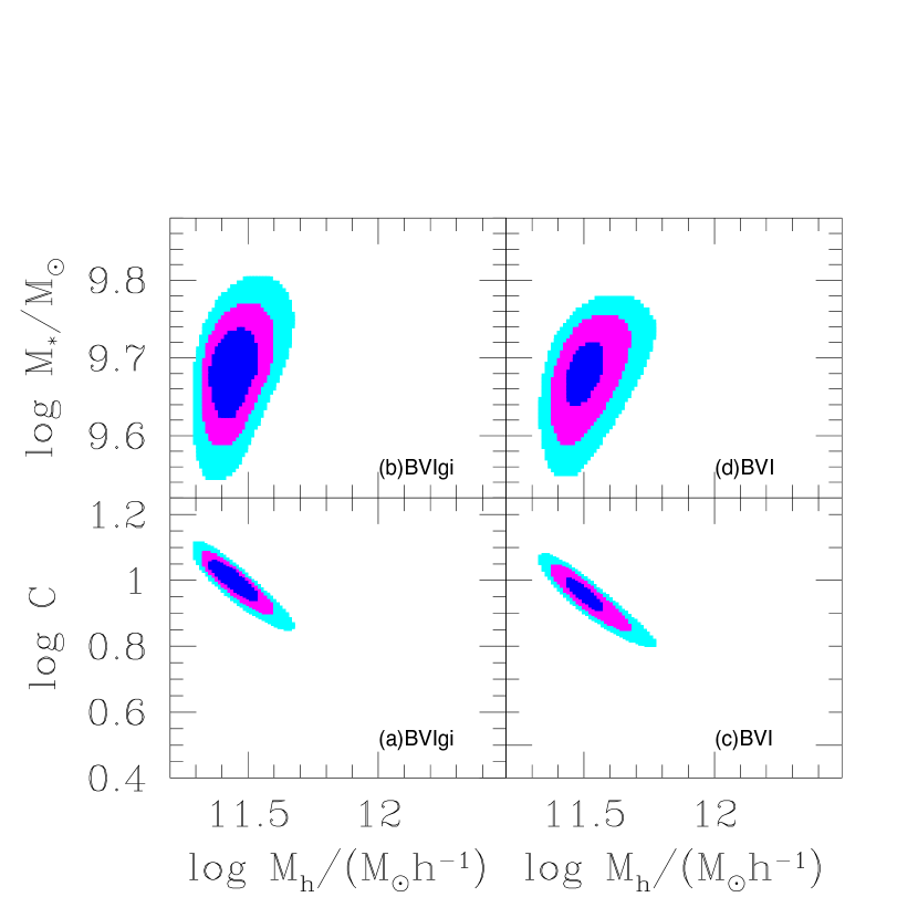
Figure 14: The 68.3$\%$ (darker regions, blue in the on-line version), 95.4$\%$ (magenta) and 99.7$\%$ (lighter regions, cyan) confidence areas in the log C–log M${}_{h}/h^{-1}$ plane and in the M_∗–M${}_{h}/h^{-1}$ plane when the probability of the dynamical fit is combined with the probability of the stellar mass surface density and of the C–M_h distribution from simulations of structure formation in a $\Lambda$CDM cosmology.The mass distribution is that given by the $BVIgi$ map for the areas shown in $(a)$ and $(b)$, and by the BVI map for the areas in $(c)$ and $(d)$.

In Table 1 (full version available in the on-line data) we display the rotation curve data, V_r, together with the azimuthal averages of the HI surface mass density, $\Sigma_{HI}$, and of the modelled surface mass density of the stars, $\Sigma_{*}$. The values of $\Sigma_{*}$ given in Table 1 correspond to the most likely value of the stellar mass distribution according to BVIgi maps and to rotation curve fit for $\Lambda$CDM halo models: M${}_{*}=4.8\times 10^{9}$ M_⊙.

Table 1: The rotation curve, the HI and stellar mass surface densities of M33

R	$\Sigma_{HI}$	$\Sigma_{*}$	Vr	$\sigma_{V}$
(kpc)	M⊙ pc-2	M⊙ pc-2	km s-1	km s-1
16.5	25.	25.	140.1	5.2
…	…	….	…..	….

6.2 Core models of dark matter halos

The dark matter halo density profile proposed by Burkert (1995) is a profile commonly used to represent the family of cored density distributions (Donato et al. 2009) and it is given by:

$$\rho(R)={\rho_{B}\over(1+{R\over R_{B}})\Bigl{(}1+({R\over R_{B}})^{2}\Bigr{)}}$$ (7)

where $\rho_{B}$ is the dark matter density of the core which extends out to $R_{B}$ (core radius). The baryonic contribution to the M33 curve is declining between 5 and 10 kpc. Hence, to have an independent estimate of the dark matter density distribution according to Salucci et al. (2010) we must probe regions which are beyond 10 kpc. The extended rotation curve of M33, which increases by about 10-20$\%$ between 5 kpc and the outermost probed radius, is therefore appropriate for this purpose. We have searched the best fitting parameters to the rotation curve, $\rho_{B}$, R_B, and M_∗ (the last one within the limited range allowed by our stellar surface density maps). There are no acceptable fits if the $BVIgi$ mass map is used, since the value of the minimum $\chi^{2}$ is 3.2. We find a minimum $\chi^{2}$ of 1.34 for the BVI mass map with M${}_{*}=7.2\times 10^{9}$ M_⊙ and the following dark halo parameters:

$$R_{B}=7.5\leavevmode\nobreak\ kpc\qquad\rho_{B}=0.018\leavevmode\nobreak\ M_{\odot}\leavevmode\nobreak\ pc^{-3}$$ (8)

The best fit is shown in the bottom panel of Figure 15. Let us notice that in this galaxy we are able to probe the dark matter out to 3 times R_B. Figure 16 shows the parameters in the 95.4$\%$ and 99.7$\%$ interval. Noticeably, the core model provides acceptable fits when the stellar mass is at the upper boundary of the interval compatible with the stellar surface density map. A good quality fit for the $BVIgi$ stellar mass map with a halo core model requires lower core densities and about 10¹⁰ M_⊙ of stars, which is extreme for a galaxy like M33. This massive stellar disk implies a factor 2 higher stellar surface density than that computed here via synthesis models, unless the IMF has a Salpeter slope over the entire stellar mass range. However, despite the heavy stellar disk predicted by the cored dark matter density distribution, the central surface density of the core is compatible with the value found by Donato et al. (2009), log($\rho_{B}$ R_B/(M_⊙ pc²))=2.15$\pm 0.2$, by fitting a very large sample of rotation curves of any luminosity and Hubble type. We plan to investigate the consistency of a cored dark matter halo with the M33 baryonic distribution in more detail in a subsequent, dedicated paper.

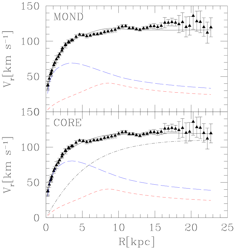
Figure 15: The rotation curve of M33 (filled triangles) and the best fitting model (solid line) for a dark matter halo with a constant density core (bottom panel) and according to MOND (top panel). The small and large dashed lines (red and blue in the on-line version) show respectively the gas and stellar disk Newtonian contributions to the rotation curves; the dark halo contribution in the bottom panel is shown with a long dashed line.

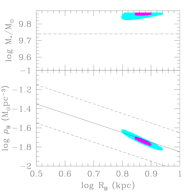
Figure 16: The 95.4$\%$ (magenta in the on-line version) and 99.7$\%$ (lighter regions, cyan) confidence areas in the log r₀ –log $\rho_{0}$ plane and in the log r₀ – log M_∗ plane relative to the rotation curve fit using a core model and the BVI mass map. In the top panel the dash-dot line indicates the most likely stellar mass according the synthesis models which rely on the BVI colors. There are no core models in the 68.3$\%$ confidence area for the BVI mass map and no acceptable core models for the $BVIgi$ mass map down to the 99.7$\%$ level. The solid line in the bottom panel indicate the inverse log$\rho_{0}$ – log r₀ correlation found by Donato et al. (2009).

6.3 Non-Newtonian dynamics without dark matter

An alternative explanation for the mass discrepancy has been proposed by Milgrom by means of the modified Newtonian dynamics or MOND (Milgrom 1983). Outside the bulk of the mass distribution, MOND predicts a much slower decrease of the (effective) gravitational potential, with respect to the Newtonian case. This is often sufficient to explain the observed non-keplerian behavior of RCs (Sanders & McGaugh 2002). According to this theory, the dynamics becomes non-Newtonian below a limiting acceleration value, ${a_{0}}$, where the effective gravitational acceleration takes the value $g=g_{n}/\mu(x)$, with ${g_{n}}$ the acceleration in Newtonian dynamics, $x=g/a_{0}$, and $\mu(x)$ is an interpolating function between the Newtonian regime and the case $g<<a_{0}$. Here, we shall use the critical acceleration value $a_{0}$ derived from the analysis of a sample of rotation curves $a_{0}=1.2\pm 0.3\times 10^{-8}$ cm s^-2 (Sanders & McGaugh 2002; Gentile et al. 2011). We have tested MOND for two choices of the interpolating function $\mu(x)$ (see Famaey & Binney 2005, for details). In particular, we have used the ‘standard’ and the ‘simple’ interpolation function and found that the former provides better fits to the M33 data. Using the ‘standard’ interpolating function, $\mu(x)=x/\sqrt{1+x^{2}}$, and the $BVIgi$ stellar surface density map, we find a minimum $\chi^{2}=1.77$ just outside the 3-$\sigma$ confidence limits. For the best fit MOND requires M${}_{*}=6.5\times 10^{9}$ M_⊙ and a${}_{0}=1.4\times 10^{-8}$ cm s^-2. A slightly lower $\chi^{2}$ (1.74) is found using the BVI mass map with M${}_{*}=5\times 10^{9}\leavevmode\nobreak\ M_{\odot}$ and a${}_{0}=1.5\times 10^{-8}$ cm s^-2. The fit provided by MOND does not improve considerably by increasing the stellar mass or the value of the critical acceleration a₀.

6.4 The baryonic fraction

The rotation curve of M33 is well fitted by a dark matter halo with a NFW density profile and a total mass of (4.4$\pm$ 1.0) 10¹¹ M_⊙. This is much larger than the halo mass which in M33 gives a baryonic fraction equal to the cosmic value, f${}_{c}=0.16$ (Spergel et al. 2003). Taking the best fitting value of stellar mass we compute a baryonic fraction of about 0.022. A baryonic fraction lower than the cosmic value is of no surprise since this is a common results in low luminosity galaxies. Feedback from star formation, such as supernovae driven outflows, is likely responsible for such a low baryonic fraction. Intergalactic filaments are in fact enriched of metals thanks to the exchange of matter between galaxies and their environment. Since the loss of gas from the galaxy will depend on the depth of the potential well, we expect that low-mass halos will be more devoid of baryons. The relationship between the stellar mass of galaxies and the mass of the dark matter halos has been derived by a statistical approach matching N-body simulated halo abundances as a function of the mass to the observed abundance of galaxies as a function of their stellar mass (Moster et al. 2010). The resulting stellar mass fraction is an increasing function of the halo mass up to 10¹² M_⊙. The analysis of the rotation curves is a different way of testing this scenario. The dark halo and stellar masses resulting from the dynamical analysis of the M33 rotation curve are compatible with the statistical relationship found by Moster et al. (2010, see their Figure 6) when scatter is taken into account. A related question is whether the presence of outflows in the early evolutionary phases of M33 might have affected the dark matter NFW profile. The recent work by Di Cintio et al. (2014, 2014a) has shown that the M33 halo mass is just at the edge of where its inner density profiles is expected to be modified by baryonic feedback, with a cuspy-like preferred inner slope.

7 Summary and conclusions

The advantage of studying a nearby galaxy such as M33 is the possibility of combining high resolution 21-cm datasets with a overwhelming amount of multifrequency data. In this work we took advantage of existing wide-field optical images in various bands to construct a map of stellar mass surface density. Two different sets of images, namely the Local Group Survey (Massey et al. 2006) and the SDSS (York & et al. 2000), have been combined in the innermost 5 kpc. Further out, these optical images are not sensitive enough to constrain the stellar surface density of M33 against variations in the background light. Thus we make use of the Spitzer 3.6 $\mu$m map and of deeper observations with large optical telescopes (e.g. Grossi et al. 2011) to estimate the stellar surface density scalelength out to the edge of the HI map. Using several methods for estimating the radially varying spatial orientation of the M33 disk, we derive the radial surface density distribution of the atomic gas and the rotation curve. By extrapolating the orientation of the outermost fitted ring for a few kpc outwards, we trace the rotation curve out to R=23 kpc. The stellar and atomic gas maps, together with the available informations on the molecular gas distribution, have been used to derive the baryonic surface density perpendicular to the galactic plane with small uncertainties. The knowledge of the potential well due to the baryons constrains the dynamical analysis of the rotation curve and the dark matter halo models more tightly than previously possible. The radial distribution of the stellar mass surface density inferred from the maps and comparison with the light distribution emphasizes the importance of combining the dynamical analysis with synthesis models. In fact, the mass-to-light ratio has non-negligible radial variations in the mapped region; additionally, local variations are present in the disk such as between the arm and interarm regions.

Numerical simulations of hierarchical growth of structure in a $\Lambda$CDM cosmological model give detailed predictions of the dark matter density distribution inside the halos. The universal NFW radial profile provides an excellent fit to the M33 rotation curve. The free parameters, halo concentration and halo mass, are found to be C=9.5$\pm 1.5$ and M_h=4.3$\pm 1.0\times 10^{11}$ M_⊙, when the C–M_h relation resulting from numerical simulations (Macciò et al. 2008) and the stellar mass surface density distribution via synthesis models are taken into account. The best estimate of the stellar mass of M33 is M${}_{*}=4.8\times 10^{9}$ M_⊙, with 12$\%$ residing in the outer disk. When added to the gas this gives a baryonic fraction of order of 0.02. A comparison of this baryonic fraction with the cosmic inferred value suggests an evolutionary history which should account for a loss of a large fraction of the original baryonic content.

A naive view of the distribution of the baryons inside the NFW dark matter halo of M33, as modelled in this paper, and the rotation curve are shown in Figure 17.

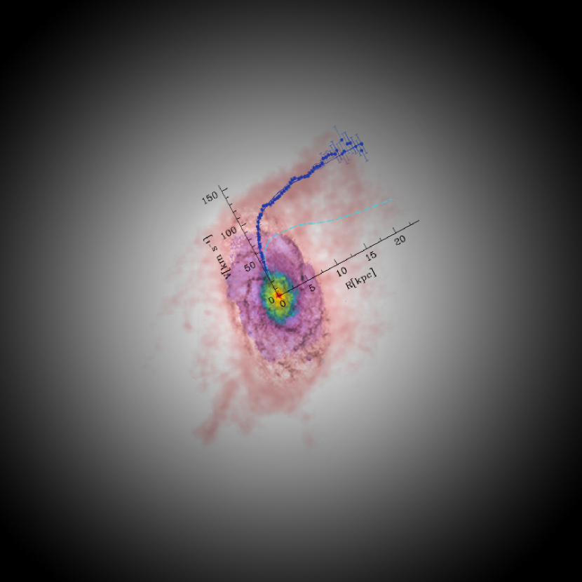
Figure 17: A naive view of M33: the inner stellar surface density (from red to magenta colors in the on-line version) superimposed to the HI gas distribution in log-scale (light pink ) are shown together with the stellar+gas contribution to the rotation curve (dashed cyan line) and with observed rotation curve (filled dots, in blue). The analysis presented in this paper has pinned down the average dark matter density distribution in the halo (light gray) which explains the observed rotation curve. The figure extrapolates the halo beyond the region analyzed in this paper in a naive smooth fashion. The total mass model fit to the rotational data, through the region analyzed in this paper, is shown by the continuous blue line.

The baryonic matter distribution in the framework of the modified Newtonian dynamic (MOND) does not provide good fits to the M33 data once the stellar content is constrained. A dark halo with a constant density core is marginally compatible with the stellar mass distribution and with the dynamical analysis of the M33 rotation curve, but requires a heavy stellar disk at the limit of the range allowed by our mass maps. The presence of a dark cuspy core in M33, as predicted by structure formation in a $\Lambda$CDM hierarchical universe, is in agreement with numerical simulation of the baryonic feedback effects on the density profiles of dark matter haloes (Di Cintio et al. 2014). For our best fit halo mass, energy from stellar feedback is insufficient to significantly alter the inner dark matter density, and the galaxy retains a cuspy profile. Given the uncertainty in the M33 stellar-to-dark matter ratio, however, we cannot exclude a slight modification of the original profile.

Having determined the stellar mass of M33 and considering a star formation rate of 0.45 M_⊙ yr^-1 (Verley et al. 2009) at z=0, we estimate a specific star formation rate (SSFR) of about 10^-10 yr^-1, in agreement with the value inferred for large galaxy samples at z=0 and by multi-epoch abundance matching models (e.g. Moster et al. 2013). A future analysis of the map of the SSFR of M33, in the framework of a chemical evolution model which takes into account gas outflow and inflow (according to the inferred dark halo mass) and reproduces the observed metallicity gradients (Magrini et al. 2010), will provide useful insights on the star formation history and, more in general, on galaxy evolutionary models.

Appendix A The tilted-ring model

To better constrain the disk orientation using the VLA+GBT 21-cm datacube we first smooth spatially the data described in the previous section at 130 arcsec resolution in order to gain sensitivity. At this spatial resolution, we reach a brightness sensitivity of 0.25 K. Considering a typical signal width of 20 km s^-1 our sensitivity should be appropriate for detecting HI gas at column densities as low as 10¹⁹ cm^-2. To determine the disk orientation, we compare the tilted ring models directly against the full spectral database considering channels 12.88 km s^-1 wide (rather than fitting the moments of the flux distribution). The cube consists of 2475 positions (i.e. pixels $40\times 40$ arcsec² wide) in which 21-cm emission has been detected, and for each position we have 25 velocity channels covering from -20 to -342 km s^-1 heliocentric velocities. We summarize below the main features of our method.

We use 110 tilted concentric rings in circular rotation around the center to represent the overall distribution of HI. Each ring is characterized by its radius $R$ and by 7 additional parameters: the H I surface density $S_{HI}$, the circular velocity $V_{c}$, the inclination $i$ and the position angle PA with respect to the line of sight, the systemic velocity $V_{sys}$ and the position shifts of the orbital centers with respect to the galaxy center ($\Delta x_{c},\Delta y_{c}$). These last 3 parameters allow the rings to be non concentric and to have velocity shifts with respect to the systemic due to local perturbations (such as gas outflowing or infalling into the ring or M31 tidal pull). Of these large set of rings we allow only the parameters of 11 equally spaced rings, called the ”free” rings, to vary independently. We set the properties of the 1st innermost free ring to be the same as those of the 2nd ring (because due to its small size it turns out to be highly unconstrained) and we keep the free rings to be the 11,22,33…110th ring. The properties of rings between each of the free ring radii were then linearly interpolated. Each of the 7 parameters of the 10 free rings were allowed to vary. We assume that the emission is characterized by a Gaussian line of width $w$, which is an addition free parameter of the model, centered at V_c. We compute the 21-cm emission along each ring as viewed from our line of sight, and the synthetic spectrum at each pixel by convolving the emission from various ring pieces with the beam pattern. We then test how well the synthetic and observed spectra match by comparing the flux densities in 25 velocity channels. With this method we naturally account for the possibility that the line flux in a pixel might result from the superposition along the line of sight of emission from different rings. As initial guess for the free parameters of the tilted ring model we follow the results of Corbelli & Schneider (1997).

The assignment of a measure of goodness of the fit is done following two methods: the ’shape’ and the ’v-mean’ method. In the shape method we minimize a $\chi^{2}$ given by the sum of two terms, the flux and the shape term. The flux term is set by the difference between the observed and modeled fluxes in each pixel. The shape term retains information about the line shape only, that are lost when just the first few moments are examined. This is essential in the regions of M33 where the emission is non-gaussian, for example when the velocity distribution of the gas is bimodal (this is indeed the case for some regions in the outer disk of M33, see CS). The shape term is given by the difference between the observed and the normalized modeled fluxes in each pixel and for every spectral channel. The normalized model spectrum is the flux predicted by the model in a given channel multiplied by the ratio of the observed to model integrated emission. In doing so the shape term is no longer dependent on the total flux. The shape term is computed only for pixels with flux larger than 0.2 Jy km s^-1/beam i.e. N${}_{HI}\geq 1.3\times 10^{19}$ cm^-2. The error for the shape term is the rms in the baselined spectra, $\sigma_{n,i}$, which is the experimental uncertainty on the flux in the $i$-channel at the $n$-pixel. The noise in each channel of the datacube, $\sigma_{ch}$, is uniform and estimated to be 0.0117 Jy/beam/channel. As suggested by Corbelli & Schneider (1997) we estimate $\sigma_{n,i}$ as:

$$\sigma_{n,i}=2{w_{i}\times\sigma_{ch}\over\sqrt{w_{i}/2.57}}$$ (9)

where $w_{i}=12.88$ km s^-1 is the width of the channel used to compare the data with the model and 2.57 km s^-1 is the database channel width. The flux term is affected by the uncertainty on the integrated flux and by calibration uncertainties, proportional to the flux. The calibration error forces the minimization to be sensitive to weak-line regions and is 5$\%$. The resultant reduced $\chi^{2}$ formula is the following:

$$\chi^{2}_{shape}={1\over{N-N_{f}}}\sum_{n=1}^{N}\bigg{\{}{(I_{n}^{mod}-I_{n}^{obs})^{2}\over 25\sigma_{n,i}^{2}+(0.05I_{n}^{obs})^{2}}$$ (10)

$$+{1\over 25}\sum_{i=1}^{25}{[(I_{n}^{obs}/I_{n}^{mod})I_{n,i}^{mod}-I_{n,i}^{obs}]^{2}\over\sigma_{n,i}^{2}}\bigg{\}}\\$$ (11)

where N is the number of pixels (2475) and N_f is the number of free parameters (71 for our basic model), leaving a large number of degrees of freedom. Given the difficulty in finding a unique minimum we use a two step method to converge toward the minimal solution. Since some of the parameters might be correlated we begin by searching for minima over a grid of the parameters surrounding our first guess. We carried out several optimization attempts under a variety of initial conditions and with different orderings for adjusting the parameters. After iterating to smaller ranges of variation, we choose the parameter values which gives the minimum $\chi^{2}$. In the second step we check the minimal solution by applying a technique of partial minima. We evaluate the $\chi^{2}$ by varying each parameter separately. We checked our solution by surrounding the galaxy with zero-flux observations for stabilizing the outermost ring. It is important to notice that the flux and the shape term give a similar contribution to the minimum $\chi^{2}$ value.

In the second method we determine a solution using the deviations of the integrated flux and of the intensity-weighted mean velocity along the line of sight at each pixel. We carried this out with another two-step procedure, allowing all 71 parameters to be varied. We start by keeping the ring centers and systemic velocity fixed; then the rings centers and velocities are considered as free parameters in the minimization as well. In order to keep the model sensitive to variations of parameters of the outermost rings, each pixel in the map is assigned equal weight. Pixels with higher or lower 21-cm surface brightness contribute equally to determine the global goodness of the model fit. Since the original data has a velocity resolution of 1.25 km s^-1, we arbitrarily set $\sigma_{m}$, the uncertainty in the mean velocity, equal to the width of about 5 channels ($\sim$6 km s^-1). This is simply a scaling factor which gives similar weight to the two terms in the $\chi^{2}$ formula. The equation below defines the reduced $\chi^{2}$ of the v-mean method:

$$\chi^{2}_{mean}={1\over{N-N_{f}}}\sum_{n=1}^{N}\bigg{\{}{(I_{n}^{mod}-I_{n}^{obs})^{2}\over 25\sigma_{n,i}^{2}+(0.05I_{n}^{obs})^{2}}$$ (12)

$$+(V^{mod}_{n}-V^{obs}_{n})^{2}/\sigma_{m}^{2}$$ (13)

where V_mod is the mean velocity predicted by the tilted ring model at the pixel $n$.

Given the large number of degrees of freedom, the increase of $\chi^{2}$ corresponding to 1-$\sigma$ probability interval for Poisson statistics would be very small. The $\chi^{2}$ standard deviation is of order 0.03 for the flux term and of order 0.006 for the shape term. Since the presence of local perturbations does not allow the model to approach a $\chi^{2}$ of order unity, we consider $\chi^{2}$ fractional variations corresponding to the mean value of the two terms (i.e. 2$\%$). By testing the $\chi^{2}$ variations for each variable independently we should have an indication on which ring and parameter is well constrained by the fitting procedure. Hence we first arbitrarily collect all possible sets of tilted ring models which give local minima in the $\chi^{2}$ distribution with values within 2$\%$ of the lowest $\chi^{2}$ (which is 7.3 and 6.8 for the v-mean and shape method respectively). In Figure 18 we show V_c, $\Delta$x_c, $\Delta$y_c and $\Delta$V_sys corresponding to an assortment of models whose $\chi^{2}$ is within 2$\%$ of the absolute minimum value found. The adopted systemic velocity is $V_{sys}$=-179.2 km/s. The displacements of the ring centers and systemic velocities are not very large and increase going radially outwards, as does the scatter between solutions corresponding to partial minima. The value of the velocity dispersion we find from the minimization is of order 10 km s^-1.

Figure 18: The parameters V_c, $\Delta$x_c, $\Delta$y_c and $\Delta$V_sys corresponding to an assortment of tilted ring models whose $\chi^{2}$ is within 2$\%$ of the absolute minimum value found. In the panels to the left the parameters for the v-mean minimization are shown, to the right those for the shape minimization. The continuous line connects the parameters of the best fit tilted ring models used for deriving the rotation curve.

For each minimization method we then select a tilted ring model between those with acceptable $\chi^{2}$ using the maximum North-South symmetry criterion for rotation curves relative to the two galaxy halves. The corresponding values of $i$ and PA are shown in Figure 3 of Section 4 with the relative uncertainties. The uncertainties are computed by varying one parameter of each free rings at a time, around the minimal solution until the $\chi^{2}$ increases by 2$\%$. Simultaneous parameter variations within the given uncertainties gives $\chi^{2}$ variations larger than 2$\%$. In deriving the rotation curve we take into account the uncertainties considering deconvolution models in which the inclination or PA of all the rings vary simultaneously. In this case we consider only 35$\%$ of the uncertainties displayed in Figure 3, in either PA or $i$, in order to have a $\chi^{2}$ within 2$\%$ of the minimal solution.

Appendix B Finite disk thickness corrections

The ”rotation curve” is the azimuthal component of the velocity in the equatorial plane of the disk at given galactocentric distance. However, the 21-cm spectrum observed at a certain position in an inclined disk depends not only on the azimuthal velocity in the plane but also on two additional effects: the smearing due to the extent of the telescope beam, and the vertical extension of the disk; both become more severe with increasing inclination. It is worth noticing that the tilted ring model fit runs over a smooothed database, spatially and in frequency, whose final geometrical parameters are then used to derive the rotation curve from a higher resolution datasets. Therefore instead of including disk finite thickness effects in the tilted ring models we prefer to account for this and for the beam smearing in the 21-cm spectral cube at the original resolution using a a set of numerical simulations.

We assume the gas to be in an azimuthally symmetric disk inclined with respect to the line of sight according to the tilted ring model fit. The gas radial distribution is set equal to that given by the integrated spectral profile, while the vertical one is modeled by an exponential with a folding length of 0.3 kpc. Only a disk component is considered with no allowance for a halo component (Oosterloo et al. 2007). For the beam we used a gaussian with $FWHM=20$ arcsec truncated at a radius of 24 arcsec; the channel spacing in the spectrum is 1.25 km s^-1. The input rotation curve is the one obtained by the observed peak and mean-velocities, and the random velocity is assumed to be isotropic and spatially constant with $FWHM=8.0$ km s^-1, as observed in most of the disk. We ran simulations with and without a vertical rotation lag according to Oosterloo et al. (2007).

Using the above parameters, we simulate a synthetic HI data cube. The cube is used to derive for each position the corresponding velocity, either the peak or the flux-averaged mean, and then build a simulated rotation curve. The differences between the simulated and the input rotation give the average corrections to the rotation curve as function of radius. We shall refer to these corrections as finite disk thickness corrections. They are of order 2-3 km s^-1 and reach values of 5 km s^-1 only within the innermost 200 pc. We apply these corrections to the rotational velocities.

References

- Aihara & et al. (2011) Aihara, H. & et al. 2011, ApJS, 193, 29
- Avila-Reese et al. (2001) Avila-Reese, V., Colín, P., Valenzuela, O., D’Onghia, E., & Firmani, C. 2001, ApJ, 559, 516
- Barker et al. (2011) Barker, M. K., Ferguson, A. M. N., Cole, A. A., et al. 2011, MNRAS, 410, 504
- Begeman (1987) Begeman, K. G. 1987, PhD thesis, , Kapteyn Institute, (1987)
- Bell & de Jong (2001) Bell, E. F. & de Jong, R. S. 2001, ApJ, 550, 212
- Bertin & Arnouts (1996) Bertin, E. & Arnouts, S. 1996, A&AS, 117, 393
- Bertin et al. (2002) Bertin, E., Mellier, Y., Radovich, M., et al. 2002, in Astronomical Society of the Pacific Conference Series, Vol. 281, Astronomical Data Analysis Software and Systems XI, ed. D. A. Bohlender, D. Durand, & T. H. Handley, 228
- Braun (2012) Braun, R. 2012, ApJ, 749, 87
- Braun et al. (2009) Braun, R., Thilker, D. A., Walterbos, R. A. M., & Corbelli, E. 2009, ApJ, 695, 937
- Bresolin (2011) Bresolin, F. 2011, ApJ, 730, 129
- Bruzual & Charlot (2003) Bruzual, G. & Charlot, S. 2003, MNRAS, 344, 1000
- Bullock et al. (2001) Bullock, J. S., Kolatt, T. S., Sigad, Y., et al. 2001, MNRAS, 321, 559
- Burkert (1995) Burkert, A. 1995, ApJ, 447, L25+
- Casertano (1983) Casertano, S. 1983, MNRAS, 203, 735
- Chabrier (2003) Chabrier, G. 2003, ApJ, 586, L133
- Charlot & Fall (2000) Charlot, S. & Fall, S. M. 2000, ApJ, 539, 718
- Ciardullo et al. (2004) Ciardullo, R., Durrell, P. R., Laychak, M. B., et al. 2004, ApJ, 614, 167
- Conroy & Gunn (2010) Conroy, C. & Gunn, J. E. 2010, ApJ, 712, 833
- Corbelli (2003) Corbelli, E. 2003, MNRAS, 342, 199
- Corbelli et al. (2010) Corbelli, E., Lorenzoni, S., Walterbos, R., Braun, R., & Thilker, D. 2010, A&A, 511, A89
- Corbelli & Salpeter (1993) Corbelli, E. & Salpeter, E. E. 1993, ApJ, 419, 104
- Corbelli & Salucci (2000) Corbelli, E. & Salucci, P. 2000, MNRAS, 311, 441
- Corbelli & Salucci (2007) Corbelli, E. & Salucci, P. 2007, MNRAS, 374, 1051
- Corbelli & Schneider (1997) Corbelli, E. & Schneider, S. E. 1997, ApJ, 479, 244
- Corbelli et al. (1989) Corbelli, E., Schneider, S. E., & Salpeter, E. E. 1989, AJ, 97, 390
- Corbelli & Walterbos (2007) Corbelli, E. & Walterbos, R. A. M. 2007, ApJ, 669, 315
- da Cunha et al. (2008) da Cunha, E., Charlot, S., & Elbaz, D. 2008, MNRAS, 388, 1595
- Davidge et al. (2011) Davidge, T. J., Puzia, T. H., & McConnachie, A. W. 2011, ApJ, 728, L23
- de Blok et al. (2001) de Blok, W. J. G., McGaugh, S. S., Bosma, A., & Rubin, V. C. 2001, ApJ, 552, L23
- de Blok et al. (2008) de Blok, W. J. G., Walter, F., Brinks, E., et al. 2008, AJ, 136, 2648
- Di Cintio et al. (2014a) Di Cintio, A., Brook, C. B., Dutton, A. A., et al. 2014a, MNRAS, 441, 2986
- Di Cintio et al. (2014) Di Cintio, A., Brook, C. B., Macciò, A. V., et al. 2014, MNRAS, 437, 415
- Donato et al. (2009) Donato, F., Gentile, G., Salucci, P., et al. 2009, MNRAS, 397, 1169
- Druard et al. (2014) Druard, C., Braine, J., Schuster, K. F., et al. 2014, ArXiv e-prints
- Eke et al. (2001) Eke, V. R., Navarro, J. F., & Steinmetz, M. 2001, ApJ, 554, 114
- Famaey & Binney (2005) Famaey, B. & Binney, J. 2005, MNRAS, 363, 603
- Freedman et al. (1991) Freedman, W. L., Wilson, C. D., & Madore, B. F. 1991, ApJ, 372, 455
- Gallazzi & Bell (2009) Gallazzi, A. & Bell, E. F. 2009, ApJS, 185, 253
- Gallazzi et al. (2005) Gallazzi, A., Charlot, S., Brinchmann, J., White, S. D. M., & Tremonti, C. A. 2005, MNRAS, 362, 41
- Gentile et al. (2005) Gentile, G., Burkert, A., Salucci, P., Klein, U., & Walter, F. 2005, ApJ, 634, L145
- Gentile et al. (2011) Gentile, G., Famaey, B., & de Blok, W. J. G. 2011, A&A, 527, A76
- Gentile et al. (2007) Gentile, G., Salucci, P., Klein, U., & Granato, G. L. 2007, MNRAS, 375, 199
- Gentile et al. (2004) Gentile, G., Salucci, P., Klein, U., Vergani, D., & Kalberla, P. 2004, MNRAS, 351, 903
- Gieren et al. (2013) Gieren, W., Górski, M., Pietrzyński, G., et al. 2013, ApJ, 773, 69
- Gnedin & Zhao (2002) Gnedin, O. Y. & Zhao, H. 2002, MNRAS, 333, 299
- González Delgado et al. (2014) González Delgado, R. M., Pérez, E., Cid Fernandes, R., et al. 2014, A&A, 562, A47
- Governato et al. (2010) Governato, F., Brook, C., Mayer, L., et al. 2010, Nature, 463, 203
- Governato et al. (2009) Governato, F., Brook, C. B., Brooks, A. M., et al. 2009, MNRAS, 398, 312
- Gratier et al. (2010) Gratier, P., Braine, J., Rodriguez-Fernandez, N. J., et al. 2010, A&A, 522, A3
- Grossi et al. (2008) Grossi, M., Giovanardi, C., Corbelli, E., et al. 2008, A&A, 487, 161
- Grossi et al. (2011) Grossi, M., Hwang, N., Corbelli, E., et al. 2011, A&A, 533, A91
- Huchtmeier (1978) Huchtmeier, W. K. 1978, in IAU Symposium, Vol. 77, Structure and Properties of Nearby Galaxies, ed. E. M. Berkhuijsen & R. Wielebinski, 197–200
- Józsa et al. (2007) Józsa, G. I. G., Kenn, F., Klein, U., & Oosterloo, T. A. 2007, A&A, 468, 731
- Kauffmann et al. (2003) Kauffmann, G., Heckman, T. M., White, S. D. M., et al. 2003, MNRAS, 341, 33
- Krajnović et al. (2006) Krajnović, D., Cappellari, M., de Zeeuw, P. T., & Copin, Y. 2006, MNRAS, 366, 787
- Kriek et al. (2010) Kriek, M., Labbé, I., Conroy, C., et al. 2010, ApJ, 722, L64
- Macciò et al. (2008) Macciò, A. V., Dutton, A. A., & van den Bosch, F. C. 2008, MNRAS, 391, 1940
- Macciò et al. (2007) Macciò, A. V., Dutton, A. A., van den Bosch, F. C., et al. 2007, MNRAS, 378, 55
- Magrini et al. (2007) Magrini, L., Corbelli, E., & Galli, D. 2007, A&A, 470, 843
- Magrini et al. (2010) Magrini, L., Stanghellini, L., Corbelli, E., Galli, D., & Villaver, E. 2010, A&A, 512, A63
- Marinoni et al. (1999) Marinoni, C., Monaco, P., Giuricin, G., & Costantini, B. 1999, ApJ, 521, 50
- Martinsson et al. (2013) Martinsson, T. P. K., Verheijen, M. A. W., Westfall, K. B., et al. 2013, A&A, 557, A131
- Massey et al. (2006) Massey, P., Olsen, K. A. G., Hodge, P. W., et al. 2006, AJ, 131, 2478
- McConnachie et al. (2010) McConnachie, A. W., Ferguson, A. M. N., Irwin, M. J., et al. 2010, ApJ, 723, 1038
- Milgrom (1983) Milgrom, M. 1983, ApJ, 270, 365
- Moster et al. (2013) Moster, B. P., Naab, T., & White, S. D. M. 2013, MNRAS, 428, 3121
- Moster et al. (2010) Moster, B. P., Somerville, R. S., Maulbetsch, C., et al. 2010, ApJ, 710, 903
- Navarro et al. (1996) Navarro, J. F., Frenk, C. S., & White, S. D. M. 1996, ApJ, 462, 563
- Navarro et al. (1997) Navarro, J. F., Frenk, C. S., & White, S. D. M. 1997, ApJ, 490, 493
- Oosterloo et al. (2007) Oosterloo, T., Fraternali, F., & Sancisi, R. 2007, AJ, 134, 1019
- Portinari & Salucci (2010) Portinari, L. & Salucci, P. 2010, A&A, 521, A82
- Prada et al. (2012) Prada, F., Klypin, A. A., Cuesta, A. J., Betancort-Rijo, J. E., & Primack, J. 2012, MNRAS, 423, 3018
- Putman et al. (2009) Putman, M. E., Peek, J. E. G., Muratov, A., et al. 2009, ApJ, 703, 1486
- Rhee et al. (2004) Rhee, G., Valenzuela, O., Klypin, A., Holtzman, J., & Moorthy, B. 2004, ApJ, 617, 1059
- Saburova & Zasov (2012) Saburova, A. S. & Zasov, A. V. 2012, Astronomy Letters, 38, 139
- Salim et al. (2005) Salim, S., Charlot, S., Rich, R. M., et al. 2005, ApJ, 619, L39
- Salucci et al. (2010) Salucci, P., Nesti, F., Gentile, G., & Frigerio Martins, C. 2010, A&A, 523, A83
- Sanders & McGaugh (2002) Sanders, R. H. & McGaugh, S. S. 2002, ARA&A, 40, 263
- Sharma et al. (2011) Sharma, S., Corbelli, E., Giovanardi, C., Hunt, L. K., & Palla, F. 2011, A&A, 534, A96
- Spergel et al. (2003) Spergel, D. N., Verde, L., Peiris, H. V., et al. 2003, ApJS, 148, 175
- Teuben (1995) Teuben, P. 1995, in Astronomical Society of the Pacific Conference Series, Vol. 77, Astronomical Data Analysis Software and Systems IV, ed. R. A. Shaw, H. E. Payne, & J. J. E. Hayes, 398
- Thilker et al. (2002) Thilker, D. A., Braun, R., & Walterbos, R. A. M. 2002, in Astronomical Society of the Pacific Conference Series, Vol. 276, Seeing Through the Dust: The Detection of HI and the Exploration of the ISM in Galaxies, ed. A. R. Taylor, T. L. Landecker, & A. G. Willis, 370
- Thilker et al. (2004) Thilker, D. A., Braun, R., Walterbos, R. A. M., et al. 2004, ApJ, 601, L39
- Verley et al. (2009) Verley, S., Corbelli, E., Giovanardi, C., & Hunt, L. K. 2009, A&A, 493, 453
- Verley et al. (2007) Verley, S., Hunt, L. K., Corbelli, E., & Giovanardi, C. 2007, A&A, 476, 1161
- Williams et al. (2009) Williams, B. F., Dalcanton, J. J., Dolphin, A. E., Holtzman, J., & Sarajedini, A. 2009, ApJ, 695, L15
- York & et al. (2000) York, D. G. & et al. 2000, AJ, 120, 1579
- Zibetti et al. (2009) Zibetti, S., Charlot, S., & Rix, H. 2009, MNRAS, 400, 1181
- Zibetti et al. (2013) Zibetti, S., Gallazzi, A., Charlot, S., Pierini, D., & Pasquali, A. 2013, MNRAS, 428, 1479