The effect of the number of states on the validity of credit ratings

Abstract

We explicitly test if the reliability of credit ratings depends on the total number of admissible states. We analyse open access credit rating data and show that the effect of the number of states in the dynamical properties of ratings change with time, thus giving supportive evidence that the ideal number of admissible states changes with time. We use matrix estimation methods that explicitly assume the hypothesis needed for the process to be a valid rating process. By comparing with the likelihood maximization method of matrix estimation, we quantify the ”likelihood-loss” of assuming that the process is a well grounded rating process.

1 Motivation and Scope

Credit ratings are a popular tool to evaluate credit risk and calculate the capital adequacy requirements for banks [10]. However, there is usually no explicit criteria to determine the number of states a rating scale should have. This is true for both the credit ratings published by the credit rating agencies and for the internal ratings used by banks [3]. It has been argued that the validity of the rating process as a measure of credit risk depends on it being Markov and time continuous [8]. If ratings follow criteria based on financial and economic variables, which are time continuous, then they should themselves be time continuous. If this fails, then it is possible that ratings are biased by concerns other than financial and economical ones.

In this paper, we discuss the possibility that the dynamical properties of the process change when we change the number of states. If the number of states is artificially large, there might be additional constrains to make the process stable or to ascribe the ratings. In turn, these additional constrains can affect the validity of the usual assumption that ratings are a time continuous process. On the other hand, if there are too few states, then it might be impossible to distinguish two issuers with the same rating based on their intrinsic credit risk. Furthermore, in this case, it is possible that the historical data of previous ratings might be a criterion to determine the different levels of credit risk within the same rating state, meaning that the process is not Markov.

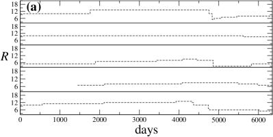
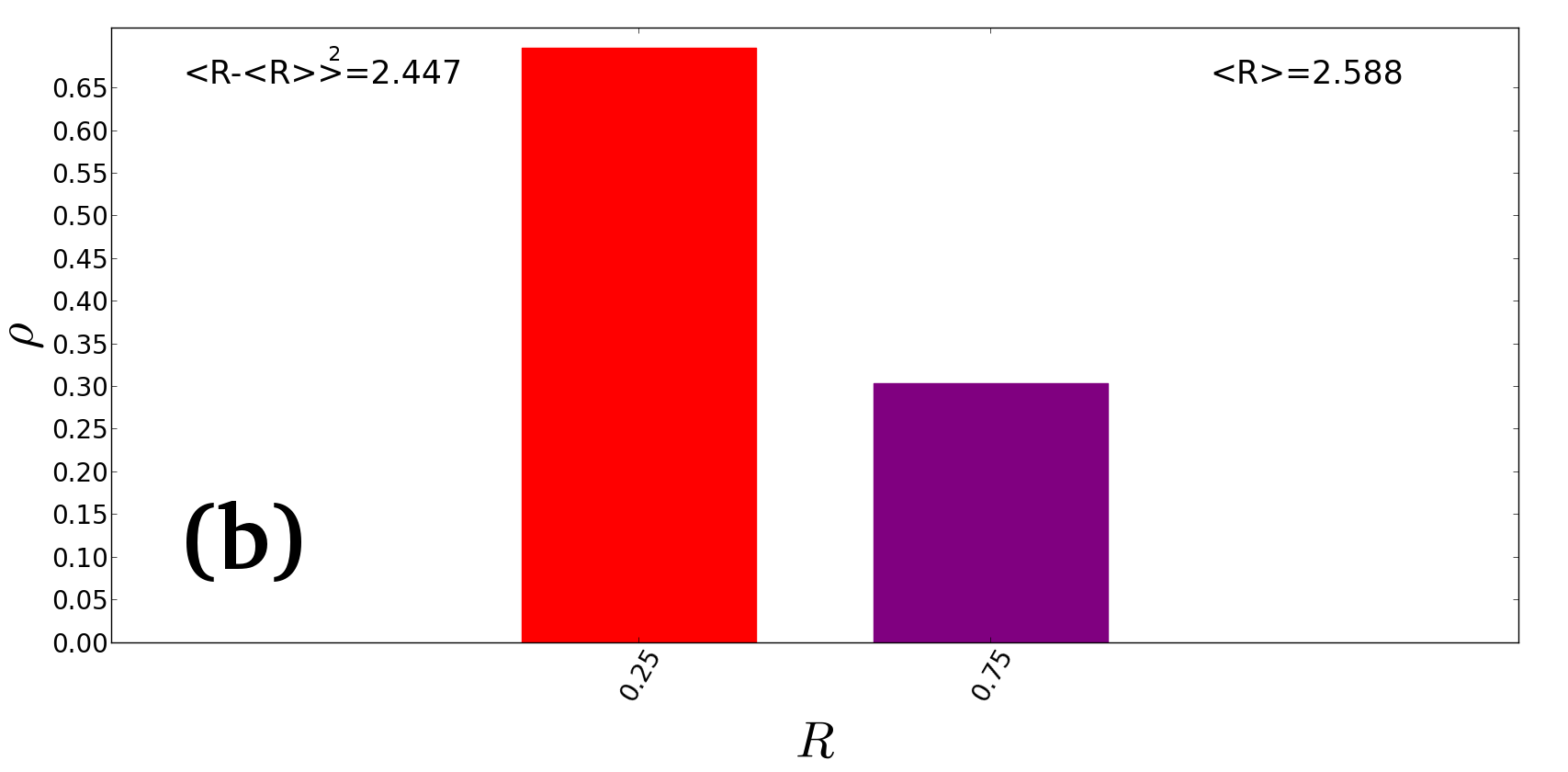
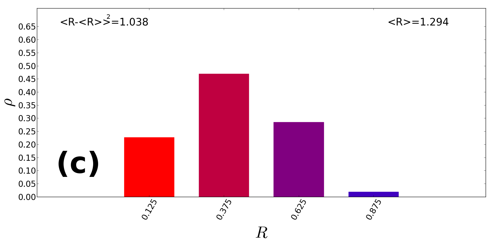
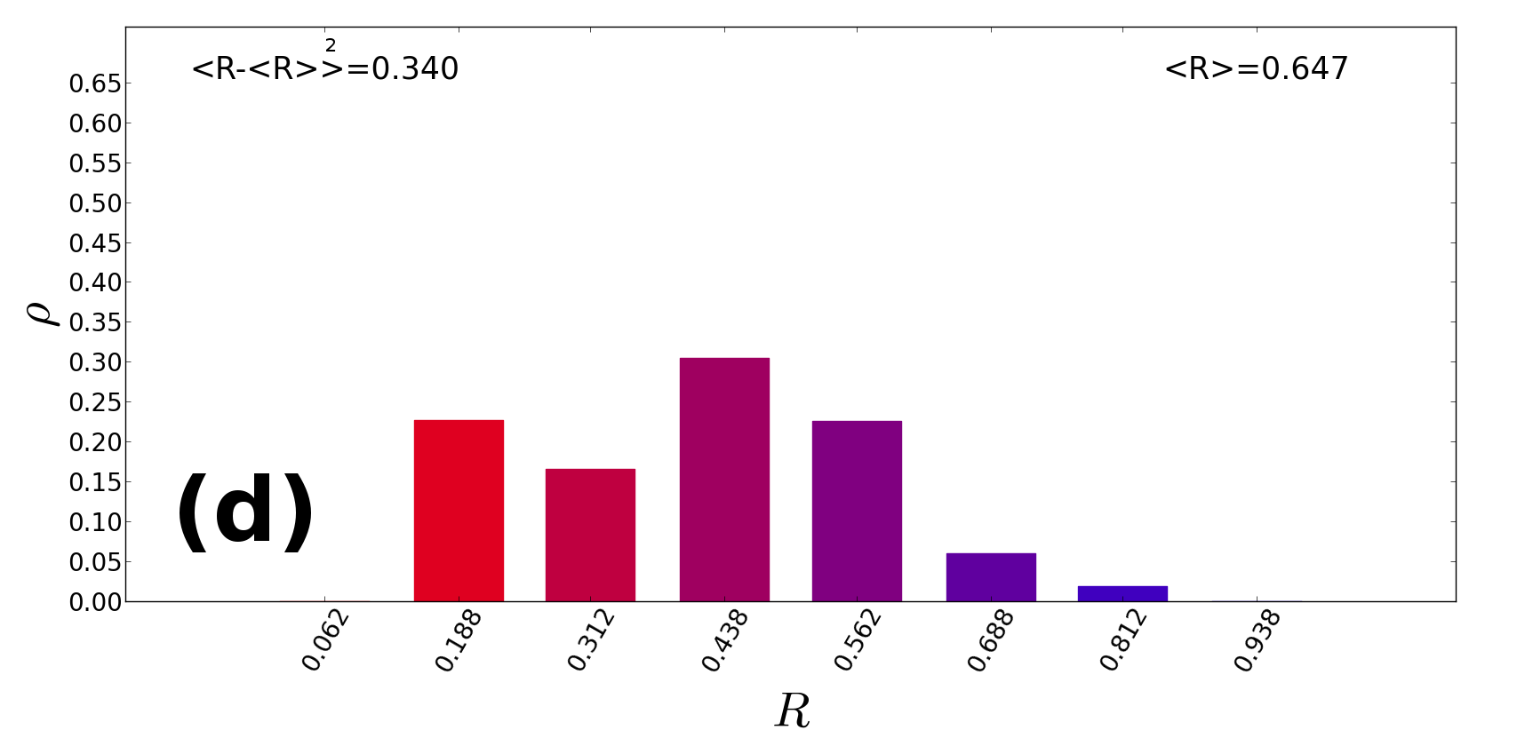
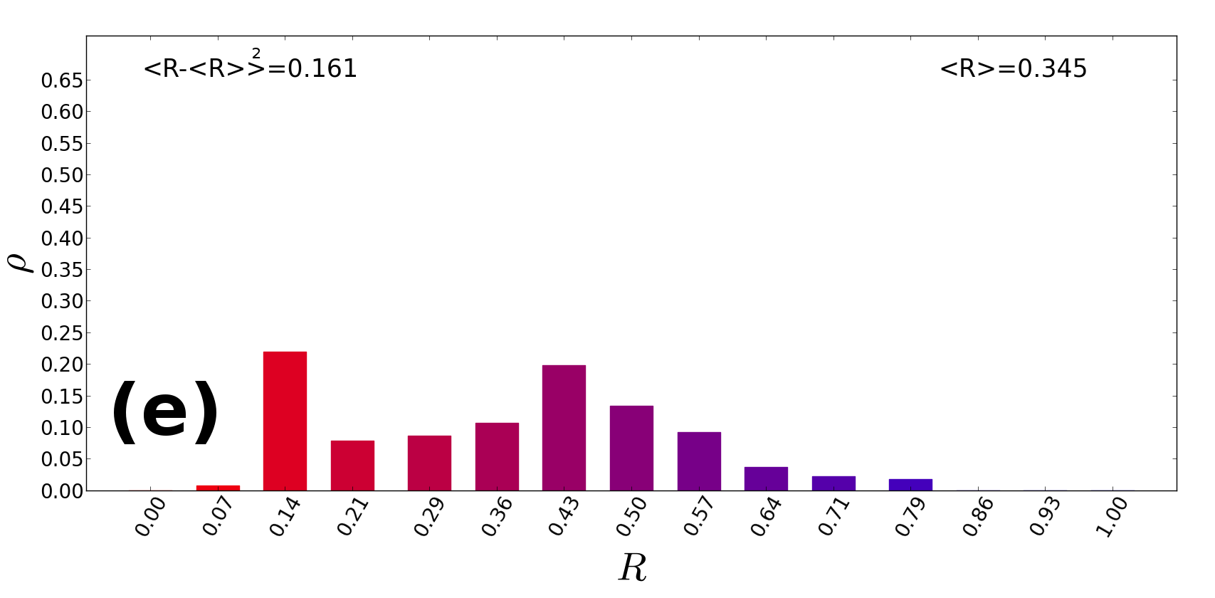
Figure 1: (a) Time series of the credit ratings of $10$ individual entities from the time when they are first rated until the present. (b-e) Histogram of rating frequencies in the first of January of 2010 for different number of states $n_{s}=\{2,4,8,15\}$.

By using different techniques to estimate a transition matrix from a finite sample of data [7], one can evaluate the dependency of the dynamical properties of ratings with the number of states. Below, we compare transition matrices calculated under different assumptions and show that the quality of the time continuity and Markov assumptions changes considerably in time. We start, in Sec. 2, by describing the empirical data collected from Moody’s. In Sec. 3 we present the theoretical background for estimating transition matrices and in Sec. 4 we describe how to test the validity of both the existence of a generator and Markov assumptions. Section 5 concludes the paper and presents some discussion of our results in the light of finance rating procedures.

2 Data description

The time series used in this paper was reconstructed by us[8] from data provided by Moodys, an influential credit rating agency, and publicly available in compliance with Rule 17g-2(d)(3) of US. SEC regulations [4]. Our data sample is the set of rating histories from the European banks, with a sample frequency of one day, starting in January 1st 2007 and ending in January 1st of 2013.

The rating class considered for our analysis is the so-called Banking Financial Strength[9], a measure of a bank’s intrinsic credit risk including factors such as franchise value, and business and asset diversification [9] and excluding external factors, such as government support. In the Financial Strength rating class there are 15 credit rating grades, represented by letters from "A" to "E" with the two possible extra suffixes "+" and "-".

Figure 1a shows several examples of individual rating histories for each entity. It can be seen that rating changes occur infrequently, with an average of $0.43$ transitions each year. We further label each state with a number ranging from $\frac{1}{2n}$ (default) to $1-\frac{1}{2n}$ (highest rating), where $n$, with $n>1$, represents the number of accessible states.

In Figs.1b-e we plot the histogram of the ratings $R$ on January 1st 2010, for $2,4,8$ and $15$ states respectively. The histograms were constructed from the original $15$-state histogram by merging pairs of adjacent states into one single state.

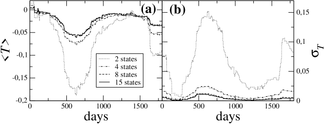
Figure 2: Comparing the sensitivity of the rating increment evolution with the number of admissible states. For $2,4,8$ and $15$ admissible states, one plots (a) the mean $\langle T(t,\tau)\rangle$ of the ratings increments, (b) the standard deviation $\sigma_{T}(t,\tau)$, both for $\tau=1$ year.

We define the rating increments as

$$T_{i}(t,\tau)=R_{i}(t)-R_{i}(t-\tau).$$ (1)

When $T_{i}(t)>0$ (resp. $<0$) it means that bank $i$ saw its rating increased (resp. decreased) during the last $\tau$ period of time. Unless stated otherwise we will use always $\tau=1$ year.

In Fig. 2 one sees that, although the first two statistical moments of $T(t,\tau)$ grow when we use less states, they have always a similar shape whatever number of admissible states is used.

3 Estimating rating transition matrices

There are three methods of extracting a transition matrix directly from a time series [6].

One is simply the normalization of the transition number matrix $\mathbf{N}$, where each entry $N(t,\tau)_{i,j}$ gives the number of transition in the desired time interval $[t-\tau,t]$. The transition matrix is then obtained by normalizing the row-sums to one:

$$(\mathbf{T}(t,\tau))_{i,j}=\frac{(N(t,\tau))_{i,j}}{\sum_{j}(N(t,\tau)_{i,j}}.$$ (2)

This estimation method is called the Cohort Method[7] and is the default method.

Another method consists in estimating the generator matrix [5],[2] $\mathbf{Q}$ directly from empirical data[7, 1]. The off-diagonal elements are empirically estimated as

$$(Q(t,\tau))_{i,j}=\frac{(N(t,\tau))_{i,j}}{\int_{t-\tau}^{t}N_{i}(t\prime)dt\prime},$$ (3)

where the number $N_{i}(t\prime)$ stands for the number of entities in state $i$ at moment $t$. The diagonal elements are calculated by forcing the row-sums of $\mathbf{Q}$ to be zero. We then calculate the transition matrix as $\mathbf{T}^{\prime}(t,\tau)=e^{\mathbf{Q}(t,\tau)}$. This estimation method is valid if and only if the underlying process is time-continuous, Markov and time-homogeneous[7].

Finally, the third method consists in using the Chapman-Kolmogorov Equation[11], which holds for any Markov process, given by

$$\bar{\mathbf{T}}(t,\tau)=\prod_{n=1}^{k}\mathbf{T}_{t-(k-i)\tau,\tau\prime},$$ (4)

where $\tau\prime=\tau/k$. This corresponds to the multiplication of matrices with a smaller non-overlapping time-window of size $\tau\prime$.

4 Comparing different estimations

In this work we want to compare all three estimations, $\mathbf{T}$, $\mathbf{T}^{\prime}$ and $\bar{\mathbf{T}}$ and quantify the difference between them. To compare them, we will use a so-called likelihood difference between the transition matrix of the default method $\mathbf{T}$ and the other two estimations:

$$d(\mathbf{T},\mathbf{T}_{other})=\frac{\sum_{i,j}(N(t,\tau))_{i,j}\left(\frac{\log{(T(t,\tau)_{i,j})}}{\log{((\mathbf{T}(t,\tau)_{other})_{i,j})}}\right)}{\sum_{i,j}(N(t,\tau))_{i,j}}\,$$ (5)

where $\mathbf{T}_{other}$ represents either the matrix $\mathbf{T}^{\prime}$ of the generator matrix estimation method or the matrix $\bar{\mathbf{T}}$ in the Chapman-Kolmogorov estimation method. This norm is particularly useful when one of the matrices maximizes of the likelihood function, which is the case for the cohort estimated matrix [7]. This way, the distance $d(\mathbf{T}_{other},\mathbf{T})$ becomes an adequate measure of the "likelihood loss" by choosing a different estimation method.

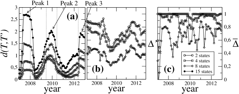
Figure 3: (a) Comparison between $\mathbf{T}$ and $\mathbf{T}\prime$, calculated over a time-window of one year, using the log-likelihood distance of the Eq. 5. (b) Comparison between the likelihood distance with $15$ states and a smaller number of states. (c) The same as (b) for the transition matrix $\overline{\mathbf{T}}$ computed from the Chapman-Kolmogorov equation.

We compare $\mathbf{T}$ with $\mathbf{T}\prime$, and $\overline{\mathbf{T}}$ with a fixed time-window of one year, and plot $d(\mathbf{T},\mathbf{T}\prime)(t)$ and $d(\mathbf{T},\overline{\mathbf{T}})(t)$ in Fig.  3. If the process is time-homogeneous, Markov and time-continuous, as one expects from a rating process [8], then the difference between $\mathbf{T}$, $\mathbf{T}\prime$ and $\overline{\mathbf{T}}$ should be white noise resulting from dealing with a finite sample.

However, when too few states are considered, e.g. only two states (good and bad), it might be possible to distinguish entities in the same state due to their history, making ratings not Markov. In general we expect the system to lose the Markov property when the “width” of each rating grade, a percentile of the maximum financial health, is bigger than the uncertainty associated to the uncertainty characteristic of the average entity’s financial health. This might be counter-balanced by the fact that when we reduce the number of states we also lose information about the system’s past. Nonetheless, when we lower the number of states, the “pure” white noise of dealing with a finite sample of data becomes lower, but the difference between matrices might become larger due to the fact that the process might not be Markov.

To see if the process is time-continuous, Markov, and time-homogeneous, we measure how correct it is to assume that a generator exists through the difference $d(\mathbf{T},\mathbf{T}\prime)$. Results are shown in Fig. 3a. In Fig. 3b one plots the normalized difference between the distances for the standard $15$ states and the fewer states cases:

$$\Delta(\mathbf{T},\mathbf{T}_{other})=\frac{d(\mathbf{T},\mathbf{T}_{other}^{(15)})-d(\mathbf{T},\mathbf{T}_{other}^{(n)})}{d(\mathbf{T},\mathbf{T}_{other}^{(15)})},$$ (6)

with $\mathbf{T}_{other}=\mathbf{T}\prime$ and with $n=2,4$ and $8$. As a notation simplification, we use $\Delta\prime=\Delta(\mathbf{T},\mathbf{T}\prime)$ and $\bar{\Delta}=\Delta(\mathbf{T},\bar{\mathbf{T}})$.

When testing the validity of the assumption of the existence of a generator, it possible to observe that the shape of $d(\mathbf{T},\mathbf{T}\prime)$ preserves most features when we change the number of states, although the scale of the different graphics change. In fact, as can be seen from Fig. 3b, all three peaks in 2007, 2009 and 2012 remain visible and occur at approximately the same time and have the same duration. Their relative strength, however, is inverted. With $15$ rating classes, the peak in 2007 is stronger than the other two, equally strong peaks in 2009 and 2012. The relative strength of the three peaks is somehow equal using the reduced sets of 8 and 4 states, whereas for two states the 2009 peak becomes strongest.

To test when the process is Markov we check when does the Chapman-Kolmogorov Equation (4) hold, and in Fig. 3c one plots a quantity $\bar{\Delta}$ using Eq. (6) but this time for using the matrices $\mathbf{T}$ and $\bar{\mathbf{T}}$. The peaks of $d(\mathbf{T},\overline{\mathbf{T}})$ occur now at the same instants as the peaks of $d(\mathbf{T},\mathbf{T}\prime)$, namely at the beginning of 2007, 2009 and 2012.

Reducing the number of states preserves the shape of the graphic, and the years at which a greater deviation occurs, but greatly diminishes the overall scale and difference between $\mathbf{T}$ and $\overline{\mathbf{T}}$. In the limit of two states, almost all information is lost.

5 Conclusions

We have used publicly available Moody’s time series of credit ratings and studied simple ways to compute the validity of the usual assumptions, regarding credit rating time series, as a function of the number of rating states.

In general, we have presented evidence that the accuracy of the time-continuous Markov time homogeneous assumptions vary not only in time but also with the number of states. Consequently, the choice of how many admissible states one should use to categorize a sample of rated entities should not be fixed in large time-spans.

Moreover, we also found that during periods when the process shows to be non-Markovian or during which no proper generator exists the choice of the number of admissible states is of importance, since the non-Markovianity and the unreliability of a generator is less pronounced when one chooses a number of admissible states smaller than the standard $15$ states.

Using empirical data for which $15$ states were prescribed it is not possible to extend this work to consider a number of admissible states larger than $15$. One may conjecture that, the choice of $15$ is better than a smaller number for detecting deviations from Markov time-continuous processes, but whether or not this is an optimal choice is an open question for future investigations.

References

References

- [1] Theodore Charitos, Peter R de Waal, and Linda C van der Gaag. Computing short-interval transition matrices of a discrete-time markov chain from partially observed data. Statistics in medicine, 27(6):905–921, 2008.
- [2] EB Davies. Embeddable markov matrices. Electronic Journal of Probability, 15:1474–1486, 2010.
- [3] Jens Grunert, Lars Norden, and Martin Weber. The role of non-financial factors in internal credit ratings. Journal of Banking & Finance, 29(2):509–531, 2005.
- [4] https://www.moodys.com/Pages/reg001004.aspx.
- [5] R.B. Israel, J.S. Rosenthal, and J.Z. Wei. Finding generators for markov chains via empirical transition matrices, with applications to credit ratings. Mathematical Finance, 11(2):245–265, 2001.
- [6] Yusuf Jafry and Til Schuermann. Measurement, estimation and comparison of credit migration matrices. Journal of Banking & Finance, 28(11):2603–2639, 2004.
- [7] David Lando and Torben M Skødeberg. Analyzing rating transitions and rating drift with continuous observations. journal of banking & finance, 26(2):423–444, 2002.
- [8] Pedro Lencastre, Frank Raischel, Pedro G Lind, and Tim Rogers. Are credit ratings time-homogeneous and markov? arXiv preprint arXiv:1403.8018, 2014.
- [9] S Moody. „moody’s rating symbols & definitions”. Moody’s Investors Service, Report, 79004(08):1–52, 2004.
- [10] Samu Peura and Esa Jokivuolle. Simulation based stress tests of banks’ regulatory capital adequacy. Journal of Banking & Finance, 28(8):1801–1824, 2004.
- [11] Hannes Risken. Fokker-Planck Equation. Springer, 1984.