Soliton scattering as a measurement tool for weak signals

Abstract

We have considered relativistic soliton dynamics governed by the sine-Gordon equation and affected by short spatial inhomogeneities of the driving force and thermal noise. Developed analytical and numerical methods for calculation of soliton scattering at the inhomogeneities allowed us to examine the scattering as a measurement tool for sensitive detection of polarity of the inhomogeneities. We have considered the superconducting fluxonic ballistic detector as an example of the device in which the soliton scattering is utilized for quantum measurements of superconducting flux qubit. We optimized the soliton dynamics for the measurement process varying the starting and the stationary soliton velocity as well as configuration of the inhomogeneities. For experimentally relevant parameters we obtained the signal-to-noise ratio above 100 reflecting good practical usability of the measurement concept.

I Introduction

Solitary waves (named solitons) preserving their shape due to a strong nonlinear interaction with the medium in which they propagate are well known from macroscopic to microscopic scales MK . One of the equations having soliton solution is the sine-Gordon (SG) one. This equation describes a variety of nonlinear systems MK ; WLLU ; snig ; Ust ; NFP ; KS ; pskm ; dna ; dna2 ; dna3 ; dna4 ; Hut ; VGS among which are superconducting devices devoted for information receiving and processing SDA ; Miki , including quantum schemes qubit ; WKU ; FSSU ; BBPH . For read out the last ones, the well known high sensitivity of superconducting detectors CB can be conjugated with evanescent back-action on the measured object using a special readout concept, e.g. the ballistic readout A . Operation principle of the ballistic readout is based on ability of a measured object to affect transport of particles by inducing scattering potential for them, which is similar to the idea of the Rutherford experiments. Due to their inherent particle-like stability joint with a wave nature, the solitons (which are the fluxons in superconducting circuits) are the natural candidates for the role of particles in the scheme. Such fluxonic detector was proposed ARS , studied HFSIS ; FSSK ; F ; SKBPK and tested experimentally FSSU ; FSWBU . It has been argued that all types of measurements known in quantum mechanics can be realized using this approach. Namely, the measurements can be done in single-shot SKBPK , weak continuous (in some literature called “non-projective”) MQ ; BVT and nearly non-demolition ARS regimes that have grown an interest in the research motivated by possibility of exploration of such fundamental scientific concepts as “wave function collapse” and decoherence.

One option of the considered measurement scheme for detection of weak magnetic field (which can be a flux qubit field) is shown in Fig. 1a. In this interferometric scheme a couple of fluxons simultaneously propagate through a couple of identical Josephson transmission lines (JTLs). The measured object, being coupled with one of the JTLs, introduces its weak magnetic field into this JTL, where it is transformed to the current dipole (the dipole of the driving force affecting the soliton motion) as shown in Fig. 1b. Fluxon scattering at this current dipole leads to deviation of its propagation time from the ones of the fluxon propagating through the reference (uncoupled) JTL. The time difference can be detected at the output comparison circuit if its magnitude is well above the noise level. The measurements, based on soliton scattering, can be realized also in frequency domain as it was done in experimental works FSSU ; F ; FSWBU .

Figure 1: (a) Fluxonic ballistic detector scheme. (b) Transformation of the qubit magnetic field into the current dipole in the JTL (blue arrows show currents induced by the field and the fluxon currents). Black arrows show fluxons. S denotes superconductor and I - isolator.

Experimental results revealed an importance of accounting for relativistic aspects of fluxon dynamics in estimation of the detector response, while theoretical works devoted to the detector mainly considered non-relativistic regime with stationary fluxon velocity HFSIS ; FSSK because of mathematical difficulties. The non-relativistic approach was also traditionally used for estimation of noise effect on fluxon dynamics in digital superconducting circuits RL ; Ter ; Ter2 . However, the recent works SKPIK ; PGK have shown that such relativistic effects as Lorenz contraction of the fluxon shape and change of its effective mass drastically affect the noise properties of the system.

In this paper we develop analytical and numerical methods for modeling of the soliton scattering at inhomogeneities of the driving force and accounting for the thermal fluctuations, comprising consideration of relativistic regime. The developed approaches allow us to calculate the signal-to-noise ratio (SNR) of the measurement procedure based on soliton scattering. For particular example of the original fluxonic ballistic detector scheme ARS we find dependences of the SNR as function of the driving force as well as the location of its inhomogeneities induced by a measured object. Tuning of the detector parameters allows us to obtain the SNR values above 100 that proves practical applicability of the considered measurement concept.

II Calculation of soliton scattering dynamics

Let us consider the SG equation describing a JTL. For superconducting phase difference $\phi$ it can be written in the following form:

$${\phi}_{tt}-{\phi}_{xx}+\sin(\phi)=-\alpha{\phi}_{t}+i+i_{f}(x,t)+i_{s}(x).$$ (1)

Here the first two terms ($-\alpha\phi_{t}$ and $i$) in the right-hand side of the equation (1) represent the energy dissipation due to tunneling of normal electrons across the barrier and the overlap bias current density providing the energy input. The next two terms ($i_{f}(x,t)$ and $i_{s}(x)$) account for the thermal fluctuations and scattering inhomogeneity of the bias current.

The components of the current densities $i$, $i_{f}$ and $i_{s}$ are normalized to the critical current density $J_{c}$. The space coordinate $x$ and the time $t$ are normalized to the Josephson penetration length $\lambda_{J}$ and to the inverse plasma frequency $\omega_{p}^{-1}$, respectively; $\alpha={\omega_{p}}/{\omega_{c}}$ is the damping coefficient, $\omega_{p}=\sqrt{2eI_{c}/\hbar C}$, $\omega_{c}=2eI_{c}R_{N}/\hbar$, $I_{c}$ is the critical current, $C$ is the JTL capacitance, $R_{N}$ is the normal state resistance. The noise correlation function is: $\left<i_{f}(x,t)i_{f}(x^{\prime},t^{\prime})\right>=2\alpha\gamma\delta(x-x^{\prime})\delta(t-t^{\prime})$, where $\gamma=I_{T}/J_{c}\lambda_{J}$ is the dimensionless noise intensity Fed ; Fed2 , $I_{T}=2ekT/\hbar$ is the thermal current, $e$ is the electron charge, $\hbar$ is the Planck constant, $k$ is the Boltzmann constant and $T$ is the temperature. If the scattering inhomogeneity has the width much less than the fluxon characteristic size $\lambda_{J}$, the corresponding term can be expressed as $i_{s}(x)=\mu\delta(x-x_{c})$, where $\mu$ is the amplitude and $x_{c}$ is the central coordinate of the inhomogeneity.

II.1 Analytical approach.

Analytical description of the soliton scattering dynamics can be developed if all the perturbation terms in the equation (1) are small: $\alpha,i,i_{f},i_{s}\ll 1$. In this case one can use the collective coordinate perturbation theory developed by McLaughlin and Scott McS to obtain the system of nonlinear differential equations for the soliton velocity $u$ and its central coordinate $X$ (the details of the calculations are summarized in the Appendix):

$$\frac{du}{dt}=-\alpha u(1-u^{2})-\frac{1}{4}[\pi i+\xi(t)](1-u^{2})^{3/2}\\ -\frac{1}{4}(1-u^{2})\mu\operatorname{sech}(\theta),$$ (2a)

$$\frac{dX}{dt}=u-\frac{1}{4}u\sqrt{1-u^{2}}\mu\theta\operatorname{sech}(\theta),$$ (2b)

where $\theta=(X-x_{c})/\sqrt{1-u^{2}}$, the velocity $u$ is normalized to the Swihart velocity $c=w_{p}\lambda_{J}$, $X$ is normalized to $\lambda_{J}$, and the noise intensity JKMMSS $\left<\xi(t)\xi(t^{\prime})\right>=\alpha\gamma(1-u^{2})^{-1/4}\delta(t-t^{\prime})$.

This system is too complex to be solved directly. However, one can find the desired dependences successively considering the scattering and the noise effect as perturbations to the solution governed by constant energy gain and loss ($i$ and $\alpha$). This solution (for $\mu,\xi=0$ in the system (2)) describing the soliton velocity relaxation process conditioned by $i/\alpha$ ratio is as follows:

$$u^{rel}(t)=\operatorname{sgn}(p)\left(1+p^{-2}\right)^{-1/2},$$ (3a)

$$X^{rel}(t)=u_{st}(t-t_{0})+\frac{u_{st}\ln(A_{1})-\ln(A_{2})}{\alpha}+C,$$ (3b)

where

$$p=\left(\beta+u^{rel}(t_{0})/\sqrt{1-u^{rel}(t_{0})^{2}}\right)e^{-\alpha(t-t_{0})}-\beta,$$ (4)

is the soliton momentum,

$$A_{1}=p\left(\sqrt{\beta^{2}+1}\sqrt{1+p^{-2}}\operatorname{sgn}(p)-\beta\right)+1,\\ A_{2}=p\left(\sqrt{1+p^{-2}}\operatorname{sgn}(p)+1\right),$$ (5)

$C$ is constant

$$C=X^{rel}(t_{0})-\frac{1}{\alpha}\biggl{(}u_{st}\ln{\textstyle\left[\frac{\sqrt{\beta^{2}+1}-\beta u^{rel}(t_{0})}{\sqrt{1-u^{rel}(t_{0})^{2}}}+1\right]}\\ -\ln{\textstyle\left[\frac{1+|u^{rel}(t_{0})|}{\sqrt{1-u^{rel}(t_{0})^{2}}}\right]}\operatorname{sgn}(u^{rel}(t_{0}))\biggr{)},$$ (6)

$u_{st}$ is the soliton stationary velocity

$$u_{st}=-\operatorname{sgn}(\beta)(1+\beta^{-2})^{-1/2},$$ (7)

parameters $t_{0}$, $X^{rel}(t_{0})$, $u^{rel}(t_{0})$ are the starting conditions, $\beta=\pi i/4\alpha$. From equation (4) it is seen that the soliton velocity relaxation rate is determined by the damping.

Next, we account for the perturbation provided by the scattering assuming the ballistic regime: $i,\alpha,\xi=0$. Approximate solution of the system (2) in this case has the form:

$$u^{sc}(\theta)=\operatorname{sgn}(u_{0})\\ \times\sqrt{1-\frac{1-u_{0}^{2}}{\left[1-\frac{\mu}{2}\sqrt{1-u_{0}^{2}}\left(\arctan\left[\tanh\left(\frac{\theta}{2}\right)\right]+c_{\pm\infty}\right)\right]^{2}}},$$ (8a)

$$X^{sc}(\theta)=\\ \frac{\theta\sqrt{1-u_{0}^{2}}}{1-\frac{\mu}{2}\sqrt{1-u_{0}^{2}}\left(\arctan\left[\tanh\left(\frac{\theta}{2}\right)\right]+c_{\pm\infty}\right)}+x_{c},$$ (8b)

where $c_{\pm\infty}$ is constant corresponding to solutions for incident ($c_{-\infty}=\pi/4$) and scattered ($c_{+\infty}=-\pi/4$) soliton for $u_{0}>0$, and vice versa for the negative velocity $u_{0}<0$.

For an incident soliton, which ballistically propagates with velocity $u_{0}$, the scattering provides a step of the velocity

$$u_{0}\rightarrow\operatorname{sgn}(u_{0})\sqrt{1-\frac{1-u^{2}_{0}}{\left(1-\operatorname{sgn}(u_{0})\frac{\mu\pi}{4}\sqrt{1-u^{2}_{0}}\right)^{2}}}$$ (9)

centered at $\theta=0$. According to the equation (8b) this step appears as a bend on the coordinate dependence

$$X\rightarrow\frac{X-x_{c}}{1-\operatorname{sgn}(u_{0})\frac{\mu\pi}{4}\sqrt{1-u^{2}_{0}}}+x_{c}.$$ (10)

Soliton velocity relaxation to its stationary value can be taken into account by using the solution (3) in the system (8): $u_{0}=u^{rel}$ and $\theta=(X^{rel}-x_{c})/\sqrt{1-(u^{rel})^{2}}$. The moment of the scattering $t^{sc}$ then can be estimated from the equation $X^{rel}(t^{sc})=x_{c}$, so

$$t^{sc}=\int_{t_{0}}^{\infty}H(u^{rel}(t))-\operatorname{sgn}(u^{rel}(t))H(X^{rel}(t)-x_{c})dt+t_{0},$$ (11)

where $H(x)$ is the Heaviside step function.

Since the scattering perturbs the relaxation dynamics of an incident soliton, the solution governed by the initial starting conditions $t_{0}$, $X^{rel}(t_{0})$, $u^{rel}(t_{0})$ can be used in the system (8) only up to the time $t^{sc}$ (for $t<t^{sc}$). After this time ($t\geq t^{sc}$) one should use the solution for a scattered soliton with appropriate starting conditions: $t^{sc}$, $X^{rel}(t^{sc})=x_{c}$ and $u^{rel}(t^{sc})$ equal to the shifted velocity defined by the right-hand side of the expression (9), where $u_{0}=\lim_{t\to t^{sc}}u^{rel}(t)$ is adopted from the incident soliton solution for crosslinking.

To account for the effect of noise, we can consider the soliton as a massive Brownian particle but with the time dependent noise intensity PGK . We omit the terms with $\mu$ in the system (2) and assume that the velocity in the factors that reflect the relativistic effects ($(1-u^{2})$ and $(1-u^{2})^{3/2}$) does not significantly fluctuate in the low noise limit, so $u$ is substituted for the found $u^{sc}(t)$ there. For further simplification we consider some fixed relativistic decrease of the damping, substituting $u^{sc}(t)$ in the factor $(1-(u^{sc})^{2})$ in front of the damping term for the average velocity $\left<u^{sc}(t)\right>$ (which derivation will be outlined below), so the effective damping is $\alpha^{*}=\alpha(1-\left<u^{sc}\right>^{2})$. Using these approximations, for Gaussian noise $\xi(t)$ we find the variance $D(t)$ and the corresponding probability $P(t)$ to find the soliton inside the segment of the length $L$ in the following form:

$$D(t)=\frac{\gamma}{4\alpha^{*}}\int_{t_{0}}^{t}\left(1-2e^{-\alpha^{*}t^{\prime}}+e^{-2\alpha^{*}t^{\prime}}\right)\\ \times\left[1-(u^{sc}(t^{\prime}))^{2}\right]^{5/2}dt^{\prime},$$ (12)

$$P(t)=1-\frac{1}{2}\operatorname{erfc}\left[\left(L-X^{sc}(t)\right)/\sqrt{2D(t)}\right].$$ (13)

These equations allow obtaining the mean soliton propagation time $\tau$ through the segment and its standard deviation $\sigma$ (jitter) using the notion of the integral relaxation time IntRel :

$$\begin{matrix}{\tau=\int_{t_{0}}^{\infty}P(t)dt,}&&{\sigma=\sqrt{2\int_{t_{0}}^{\infty}tP(t)dt-\tau^{2}}}.\end{matrix}$$ (14)

In the limit $D(t)\rightarrow 0$ the equations (13), (14) serve for estimation of the propagation time without noise and corresponding average soliton velocity $\left<u^{sc}\right>$, which in turn is used for calculation of the effective damping $\alpha^{*}$.

Finally, the SNR of the measurement process based on soliton scattering can be calculated. For example, if the measurement implies comparison between soliton propagation times with $\tau_{\mu}$ and without $\tau_{0}$ scattering, then the SNR is:

$$SNR=\frac{|\Delta\tau|}{\sigma_{\Sigma}}=\frac{|\tau_{\mu}-\tau_{0}|}{\sqrt{\sigma_{\mu}^{2}+\sigma_{0}^{2}}},$$ (15)

where $\sigma_{\mu,0}$ correspond to the mean times $\tau_{\mu,0}$.

II.2 General method.

The described analytical approach can be generalized for any number of inhomogeneities of the driving force. For example, the scattering at a dipole can be considered as two successive scatterings at inhomogeneities spread over a distance of the dipole width $d=x_{c2}-x_{c1}$ with amplitudes of the opposite sign $\mu_{2}=-\mu_{1}$. To find solution in this case one should first obtain $u^{sc}_{1}$, $X^{sc}_{1}$ using $\mu_{1}$ and $x_{c1}$ in the system (8) and then use these equations (8) again with $\mu_{2}$, $x_{c2}$, using previously obtained $u^{sc}_{1}$, $X^{sc}_{1}$ instead of $u^{rel}$, $X^{rel}$ for incident soliton solution.

If the scattering can not be considered as a perturbation (because of high scattering amplitude or since the soliton motion can not be considered as ballistic), one should proceed with numerical calculation of the system (2) in which the last terms should be substituted in general for $-(1-u^{2})\sum_{n}\mu_{n}\operatorname{sech}(\theta_{n})/4$ and $-u\sqrt{1-u^{2}}\sum_{n}\mu_{n}\theta_{n}\operatorname{sech}(\theta_{n})/4$ in the equations for $u$ and $X$ ($n$ is the inhomogeneity number). To speed up the calculations, the fluctuational term can be omitted (if $\xi\ll 1$) in the numerical evaluations of $u(t)$ and $X(t)$. The effect of noise can be accounted further as it is described above, using equations (12)-(15).

At last, if the terms on the right-hand side of the SG equation (1) are not small, this equation should be calculated numerically itself. It is useful then to substitute the delta function in the scattering term for some smoother one, e.g. hyperbolic secant FSSU : $i_{s}(x)=\sum_{n}\mu_{n}\delta(x-x_{cn})\approx\sum_{n}\mu_{n}\operatorname{sech}[(x-x_{cn})/a_{n}]/\pi a_{n}$, where $a_{n}$ characterizes the width of the scattering inhomogeneity. The mean soliton propagation time and its standard deviation can be obtained by averaging over ensemble of realizations.

III Soliton scattering as a measurement tool of the fluxonic ballistic detector

Let us consider the original fluxonic ballistic detector scheme (see Fig. 1) to study the measurements based on soliton scattering. For verification of the presented theoretical approaches we compare their results, and furthermore design the superconducting schemes for measurements of the detector time response and its jitter. The designs are intended for fabrication by FLUXONICS foundry FLUXONICS . Fragment of one of the fabricated samples is shown in Fig. 2a.

While our measurements are in progress, we have estimated parameters of Josephson junctions which are necessary for calculations. Typical current-voltage characteristic of a serial array containing 10 test junctions is presented in Fig. 2b. According to these data, the junction quality is $R_{J}/R_{N}\simeq 20$ (where $R_{J}$ is the subgap resistance) and the damping at 4 K temperature is $\alpha\simeq 0.2$. For experimental temperatures $T\geq 50$ mK we expect a decrease in the damping value by one order HFSIS down to $\alpha\simeq 0.02$.

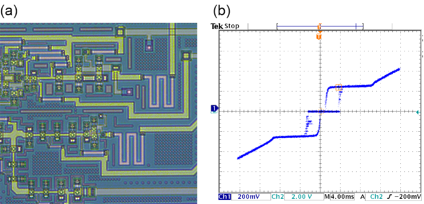
Figure 2: (a) Photo of the experimental sample fragment with digital superconducting circuits of the fluxon generator block. (b) Current-voltage characteristic of serial array containing 10 test Josephson junctions. The current scale (abscissa) is 100 $\mu$A/div, the voltage scale (ordinates) is 10 mV/div.

Our estimation gives the value of the normalized noise intensity $\gamma=10^{-5}$ at 50 mK temperature. However to speed up the numerical calculations, we mainly used the value $\gamma=10^{-3}$. This value is still much smaller than values of the other coefficients in the SG equation, so the noise effect remains weak. One should note that the time jitter and the SNR scale accurately as $\sigma_{\Sigma}\sim\sqrt{\gamma}$ and $SNR\sim 1/\sqrt{\gamma}$, respectively, that has been proven by our numerical calculations, see below.

The scattering current dipole in the considered scheme is induced by magnetically coupled flux qubit. Its amplitude is: $\pm\mu=\pm I_{p}M/2L_{cl}J_{c}\lambda_{J}$, where $\pm I_{p}$ is the persistent current circulating in the qubit (the sign corresponds to the current direction), $M$ is the mutual inductance between the qubit and the coupling loop, $L_{cl}$ is the inductance of the coupling loop. According to results of the existent experimental works F the values of the dipole amplitude is about $\mu=0.1$.

III.1 Optimization of the fluxon dynamics.

We start consideration of the measurement process based on soliton scattering from study of detector response dependences on the starting fluxon velocity and its stationary velocity. The current dipole amplitude and its width are chosen to be $\mu=0.1$ and $d=20$, respectively. The JTL length is $L=3d=60$. The dipole is placed at the center of the JTL $x_{dc}=L/2=30$. At the first step we consider the case where the starting fluxon velocity is equal to the stationary one $u(t_{0})=u_{st}$. The dipole polarity is marked as “positive” - “$+\mu$” for the case where its first pole is co-directed with the bias current (the first pole accelerates the fluxon) and “negative” - “$-\mu$” otherwise (the first pole decreases the bias current and decelerates the fluxon). The damping is assumed to be vanishing ($\alpha~{}\rightarrow~{}0$).

Fluxon scatterings at the dipole poles provide deviation of the fluxon velocity from the stationary one $\Delta u=u-u_{st}$ while fluxon moves inside the dipole, that is further detected as the time response. The dependences of the fluxon velocity on the coordinate for the both dipole polarities obtained using the presented analytical approach (solid lines) and numerical calculation of the system (2) (dots) are shown in Fig. 3a. The JTL parameters for simulation of the ballistic regime are as follows: $-i=0.0001$, $\alpha=0.0001$, $\gamma=0$. It is seen that the data obtained with the both (analytical and numerical) approaches are consistent perfectly.

Note, that fluxon deceleration can be more pronounced than acceleration due to relativistic dependence of the effective fluxon mass on its velocity. The detector response for the negative dipole polarity can be greater than for the positive one, accordingly.

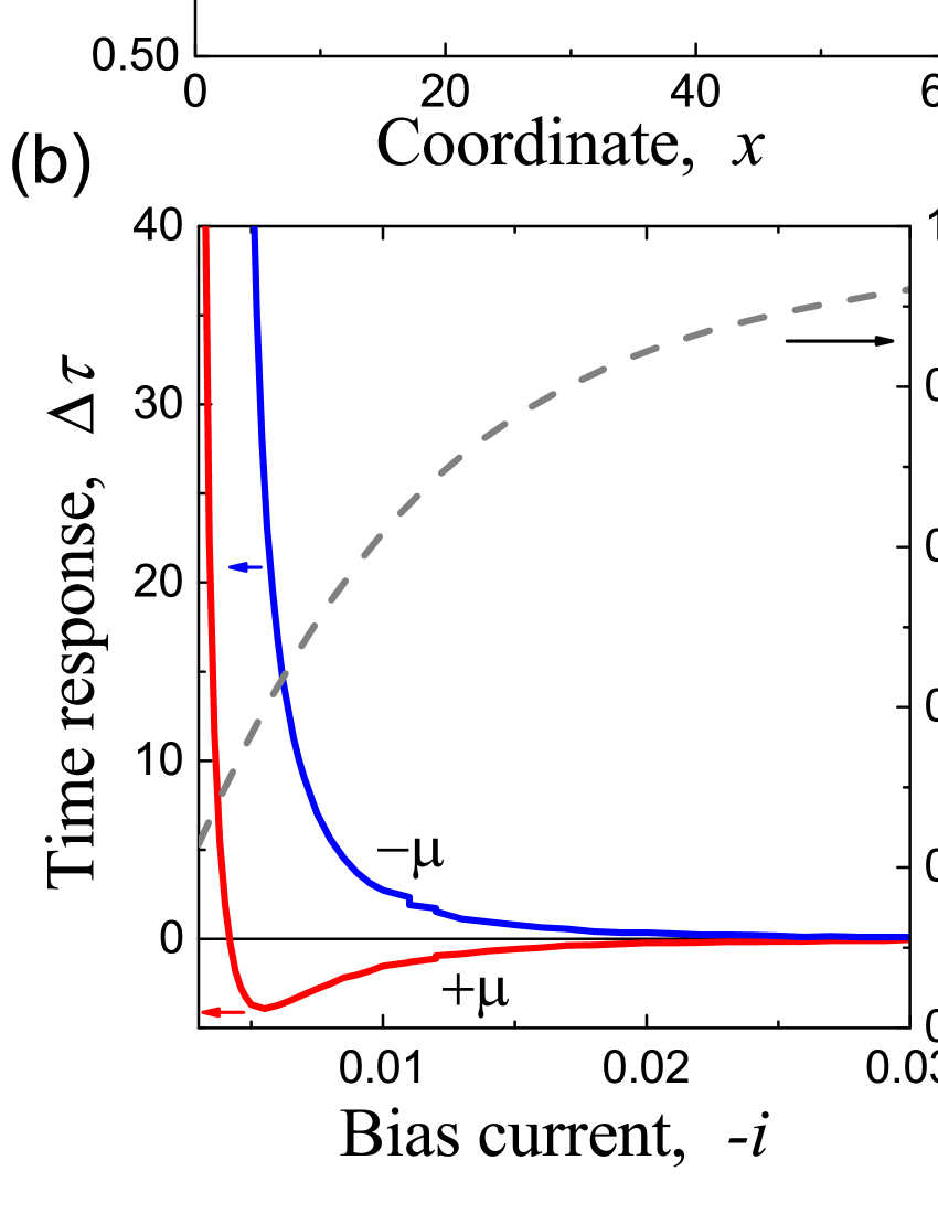
Figure 3: The fluxon velocity dependences on the coordinate for the both dipole polarities calculated using the presented analytical approach (solid curves) and numerically, using the system (2) (dotes), with fluxon starting velocity equal to the stationary one $u(t_{0})=u_{st}$ (a), and equal to zero $u(t_{0})=0$ (c). (b) The detector time responses versus the bias current for $u(t_{0})=u_{st}$ ($u_{st}$ is defined by (7) and shown by the dashed curve); $\alpha=0.01$. (d) The time responses versus the fluxon starting velocity for $-i,\alpha=0.01$; the vertical line shows the stationary velocity. The JTL and the dipole parameters are: $L=60$, $d=20$, $x_{dc}=30$, $\mu=0.1$, $\gamma=0$.

To take into account the fluxon velocity relaxation we calculate the same velocity curves for realistic parameters $-i,\alpha=0.01$, see Fig. 3a. Since the fluxon velocity becomes closer to the stationary value after the first scattering, the second scattering provides an extra compensation of the velocity deviation, so the deviation changes its sign. Thus, the relaxation serves for decrease of the detector response with the damping increase.

Fig. 3b shows the detector time response $\Delta\tau=\tau_{\mu}-\tau_{0}$ (the index $\mu$/$0$ represents the presence/absence of the scattering) calculated numerically for the same damping but for the different bias current values determining the stationary (and the starting) fluxon velocity as it follows from the expression (7). Small velocity corresponds to small effective mass that makes a fluxon more susceptible to the scattering effect increasing the response. Rapid increase of the response with the bias current decrease indicates existence of the threshold bias current. This threshold current corresponds to fluxon capturing by the first (or the second) dipole pole in the case of the negative (the positive) dipole polarity.

It is seen that the bias current maximizing the difference between the responses for the opposite dipole polarities is in the vicinity of the threshold current for the negative dipole. However, this current is impractical for implementation of series measurements. For reliable series detection (which is required for quantum measurements) one needs to shift the working bias current upward to guarantee that fluctuations will not cause the fluxon capturing. Still, there is a possibility to increase the response by tuning the starting fluxon velocity.

Fig. 3c shows the fluxon velocity curves for the same values of the bias current and the damping ($-i,\alpha=0.01$) as the ones taken for calculation of corresponding curves for nonvanishing damping shown in Fig. 3a but for zero starting velocity $u(t_{0})=0$. Fig. 3d presents the dependences of the detector time response on the starting velocity for these JTL parameters calculated numerically using the system (2). The decrease of the starting velocity in our case can lead to 5 times increase in difference between the time responses for the opposite $\mu$. We should note, that difference of signs of the time responses for the opposite dipole polarities can provide an advantage for a measurement scheme which uses digital comparator at the output.

III.2 SNR of the fluxonic ballistic detector.

In the work FSSK it was argued that the major sources of the measurement errors in the fluxonic detector are the fluxon propagation time jitter due to the thermal fluctuations and the intrinsic qubit relaxation. If the time of the measurements is much smaller than the qubit relaxation time, then the detector SNR can be calculated according to the equation (15). The total jitter $\sigma_{\Sigma}=\sqrt{\sigma_{\mu}^{2}+\sigma_{0}^{2}}$ in this equation is the standard deviation of the detector time response $\Delta\tau$ which can be obtained using the jitters corresponding to the fluxon propagations through the JTL with ($\sigma_{\mu}$) and without ($\sigma_{0}$) scattering.

To verify our theoretical approaches for evaluation of the detector parameters we calculate the detector time response, the total jitter and the SNR versus the bias current for the both dipole polarities using the three presented methods: (i) the analytical one (equations (3) - (15)), (ii) numerical calculation of the system (2) with $\xi=0$ and further accounting for the noise effect using equations (12) - (15), and (iii) numerical calculation of the SG equation (1) with averaging over ensemble of 10000 realizations. In case (iii) the simulations have been performed using the original implicit finite-difference scheme Fed ; Fed2 , which is similar to the Crank-Nicolson one, but with the account of the white noise source. The JTL and the dipole parameters are the same as before: $L=60$, $d=20$, $x_{dc}=30$, $-i,\alpha=0.01$, $\mu=0.1$, but with $\gamma=10^{-3}$. The starting fluxon velocity is equal to zero $u(t_{0})=0$. The results are shown in Fig. 4.

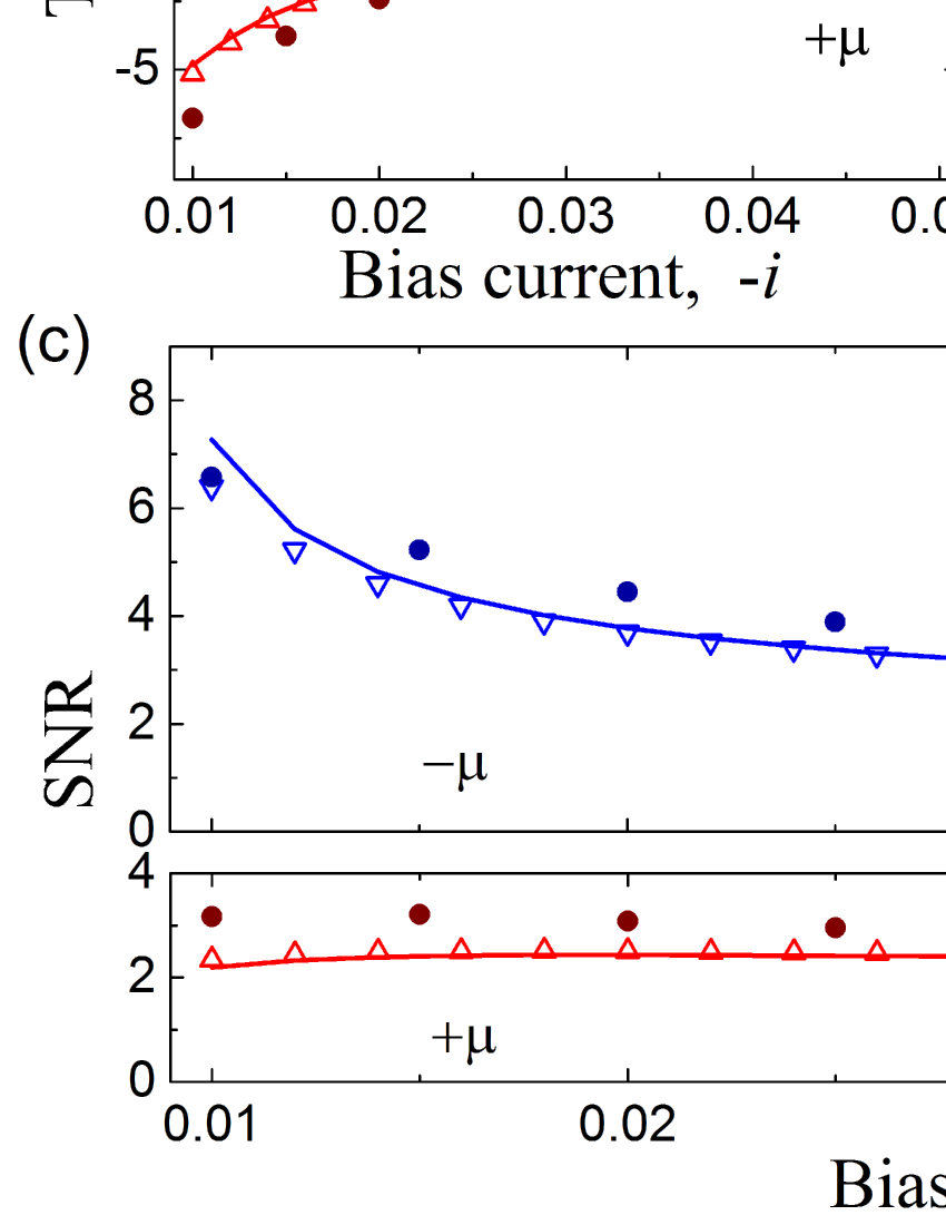
Figure 4: The detector time response (a), the total jitter (b) and the SNR (c) versus the bias current for the both dipole polarities evaluated using (i) the equations (3)-(15) (solid curves), (ii) numerical calculations of the system (2) with $\xi=0$ and further accounting for the noise effect using the equations (12)-(15) (open triangles), and (iii) numerical calculations of the SG equation (1) with averaging over ensemble of 10000 realizations (filled dots). Legend for all the panels is shown in the panel (a). $L=60$, $d=20$, $x_{dc}=30$, $-i,\alpha=0.01$, $\gamma=10^{-3}$, $\mu=0.1$, $u(t_{0})=0$.

It is seen that the data obtained using the all three methods are well consistent. Some discrepancy occurs in the range of the small bias current values where the scattering effect is especially highlighted.

The jitter increase with the bias current (and the stationary velocity) decrease can be qualitatively explained by relativistic decrease of the effective fluxon mass that makes fluxon dynamics more affected by noise. Despite this increase, for the negative dipole polarity the SNR still grows a bit toward the small bias current values (see Fig. 4c) because of more rapid increase of the time response. Contrary to this, for the positive dipole polarity the SNR curve is nearly flat because of limited growth of the time response in this case, see also Fig. 3b.

Along with the quite smooth dependences of the SNR on the bias current values corresponding to a wide range of the stationary fluxon velocities, we find more pronounced SNR dependence on the instant fluxon velocity before the scattering at the first dipole pole. Since the scattering at the second pole ends formation of the time response, we shift the second dipole pole nearly to the end of the JTL: $x_{c2}=L-5=55$. To make our results more relevant to the experiment we increase the damping value $\alpha=0.02$ as well as the dipole amplitude $\mu=0.2$ while the noise intensity and the starting fluxon velocity are hold the same $\gamma=10^{-3}$, $u(t_{0})=0$. The dependences of the SNR on the first dipole pole position for different bias currents were calculated numerically using the SG equation (1). The results for the positive and the negative dipole polarities are shown in Fig.s 5a,b respectively.

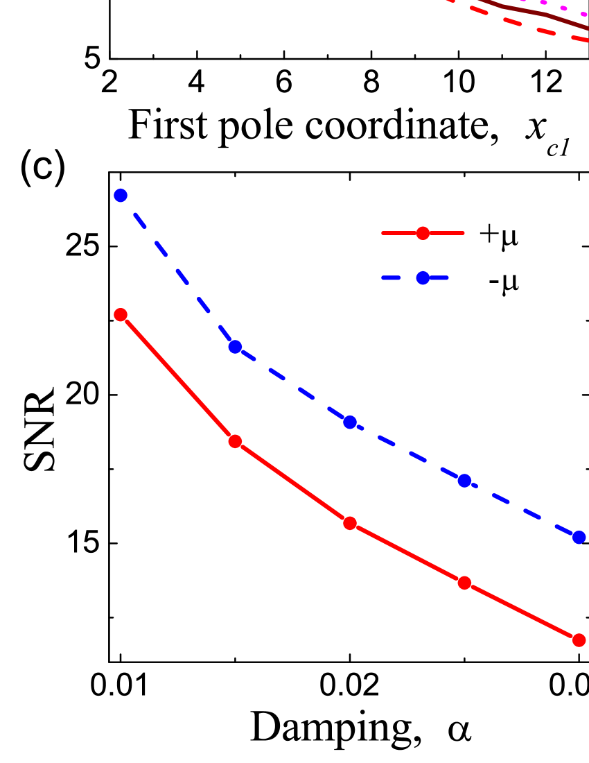
Figure 5: The detector SNR versus the first dipole pole position $x_{c1}$ in the JTL for the positive (a) and the negative (b) dipole polarities, and the bias current values $-i=0.03,~{}0.04,~{}0.05$; $x_{c2}=55$, $\alpha=0.02$, $\gamma=10^{-3}$. (c) The SNR versus the damping for the optimum bias current $-i=0.048$ at $x_{c1}=5$. (d) The SNR versus the noise intensity for the same parameters and $\alpha=0.02$. $L=60$, $\mu=0.2$, $u(t_{0})=0$.

Shift of the first dipole pole to the beginning of the JTL leads to decrease of the instant fluxon velocity and the corresponding decrease of the instant effective fluxon mass before the first scattering. Since this scattering mainly forms the time response, the SNR for the positive dipole polarity monotonically grows toward the smaller coordinate values. At the same time, the bends of the SNR curves for the negative dipole illustrates an increase of the jitter impact on the SNR in the vicinity of the threshold bias current. The tops of these bends correspond to the optimum sets of parameters for the considered measurement procedure.

Assuming that the closest location of the first dipole pole to the beginning of the JTL can be about $x_{c1}=5$, we calculated the SNR versus the damping for the optimum bias current value $-i=0.048$ corresponding to this $x_{c1}$, see Fig. 5c. It is seen that fluxon velocity relaxation provides nearly the same effect on the SNR for the both dipole polarities. Finally, to evaluate the expected SNR of the detector in the experiment, we calculated the SNR versus the noise intensity for the damping value $\alpha=0.02$ and the same bias current. The results are presented in Fig. 5d. According to our assumptions, the SNR scales as $SNR\sim\sigma_{\Sigma}^{-1}\sim\gamma^{-1/2}$ that is consistent with the results of the work SKBPK . For the estimated noise intensity $\gamma=10^{-5}$ the SNR is above 100.

IV Conclusion

In conclusion, we have developed analytical approach for calculation of relativistic dynamics of soliton scattering at weak short inhomogeneity of the driving force and account for the presence of the thermal fluctuations. We have generalized this approach for an arbitrary number of inhomogeneities as well as considered numerical approaches for calculation of the dynamics for arbitrary parameters of the system. We have considered the scattering as a measurement procedure by example of the fluxonic ballistic detector, exploiting the developed methods for its optimization. The negative role of the damping in the system for formation of the detector time response was outlined as well as using of accelerated fluxon motion leading to increase of the response was argued. Finally, we have optimized the measurement scheme configuration for experimentally relevant parameters and obtained the SNR value above 100. Since the obtained time response and its standard deviation in the frame of the detector model (taking into account only fluxon dynamics in the JTLs) are by an order of magnitudes larger than the time resolution and the thermal jitter of digital superconducting delay detector FSSK ; GP , this SNR reflects quantitatively correct estimation of attainable performance of the measurement process which is planned to be realized experimentally.

V Acknowledgements

This work was supported by Ministry of Education and Science of the Russian Federation, grant Nos. 14.Y26.31.0007, 3.2054.2014/K, RFMEFI58714X0006, RFBR projects 14-02-31002-mol$\_$a, 15-32-20362-mol$\_$a$\_$ved, 15-02-05869, Russian President grant MK-1841.2014.2, Dynasty Foundation, and in the framework of Increase Competitiveness Program of Lobachevsky NNSU under contract no. 02.B.49.21.0003.

Appendix A Calculation of soliton scattering dynamics

The perfect SG equation

$${\phi}_{tt}-{\phi}_{xx}+\sin(\phi)=0$$ (16)

can be written as a Hamiltonian system for $(\phi,\phi_{t})$ with the Hamiltonian

$$H^{SG}=\int_{-\infty}^{\infty}\left(\tfrac{1}{2}\phi^{2}_{t}+\tfrac{1}{2}\phi^{2}_{x}+1-\cos(\phi)\right)dx.$$ (17)

This system supports soliton solution which can be analytically presented by the two-parameter formula

$$\phi_{0}(x,t;x_{0},u)=4\tan^{-1}\left[\exp\pm\left(\frac{x-ut-x_{0}}{\sqrt{1-u^{2}}}\right)\right],$$ (18)

where the velocity $|u|<1$ and the coordinate $x_{0}$ are the parameters, and $\pm$ represents soliton or antisoliton state.

According to the collective coordinate perturbation analysis performed by McLaughlin and Scott McS we consider soliton dynamics in a real physical system by introducing weak structural perturbation into the perfect SG equation in the form

$${\phi}_{tt}-{\phi}_{xx}+\sin(\phi)=\epsilon f,$$ (19)

where $0\leq|\epsilon|\ll 1$, and find the response of the SG wave solution $\vec{W}={\phi\choose\phi_{t}}$ (it is assumed that initially the wave is precisely the pure soliton state $\vec{W}_{0}={\phi_{0}\choose\phi_{0t}}$ corresponding to (16)) to this perturbation in the form

$$\vec{W}=\vec{W}_{0}+\epsilon\vec{\mathfrak{w}},$$ (20)

by establishing equations for $\vec{\mathfrak{w}}$ governing modulation of the wave parameters in time.

For the considered case of a single soliton wave (18) these equations are as followsMcS :

$$\frac{du}{dt}=\mp\epsilon\tfrac{1}{4}(1-u^{2})\int_{-\infty}^{\infty}f[\phi_{0}(\Theta)]\operatorname{sech}(\Theta)dx,$$ (21a)

$$\frac{dx_{0}}{dt}=-\epsilon\tfrac{1}{4}u(1-u^{2})\int_{-\infty}^{\infty}f[\phi_{0}(\Theta)]\Theta\operatorname{sech}(\Theta)dx,$$ (21b)

where $\Theta(x,t)=\left(x-\int_{t_{0}}^{t}u(t^{\prime})dt^{\prime}-x_{0}\right)/\sqrt{1-u^{2}}$. Note, that the system (21) can be obtained just from the energy equation and the equation for the soliton momentum $p=-\frac{1}{8}\int_{-\infty}^{\infty}\phi_{0x}\phi_{0t}dx$ correspondingly:

$$\frac{dH^{SG}(\phi_{0})}{du}\frac{du}{dt}=\epsilon\int_{-\infty}^{\infty}f(\phi_{0})\phi_{0t}dx,$$ (22a)

$$\left(\frac{d}{du}\int_{-\infty}^{\infty}\phi_{0x}\phi_{0t}dx\right)\frac{dx_{0}}{dt}=\epsilon\int_{-\infty}^{\infty}f(\phi_{0})\phi_{0u}dx.$$ (22b)

Defining the central soliton coordinate as

$$X\equiv\int_{t_{0}}^{t}u(t^{\prime})dt^{\prime}+x_{0},$$ (23)

so that $\dot{X}=u+\dot{x}_{0}$, and substituting the right-hand side of the considered SG equation (1) for $\epsilon f$ in the system (21) one directly obtains the system (2).

Since for $\mu,\xi=0$ the perturbation $\epsilon f$ is the even function of $\Theta$, $\dot{x}_{0}=0$ and $\dot{X}=u$ as it follows from (21b). In this case the equation (21a) has a simple form

$$\dot{p}=-\alpha p-\pi i/4.$$ (24)

Its solution is shown by expression (4) (corresponding $u(t)$, $X(t)$ dependences are the equations (3)).

For the ballistic regime $i,\alpha,\xi=0$, the right-hand side of the system (2) contains only terms with $\theta$ and therefore it is more convenient to seek for $u$, $X$ dependences on this argument modifying the equations (2) correspondingly:

$$\frac{du}{d\theta}=-\frac{\sqrt{1-u^{2}}}{u}\frac{\frac{\mu}{4}(1-u^{2})\operatorname{sech}(\theta)}{1-\frac{\mu}{2}\sqrt{1-u^{2}}\theta\operatorname{sech}(\theta)},$$ (25a)

$$\frac{dX}{d\theta}=\frac{\sqrt{1-u^{2}}}{u}\frac{u-\frac{\mu}{4}u(1-u^{2})\theta\operatorname{sech}(\theta)}{1-\frac{\mu}{2}\sqrt{1-u^{2}}\theta\operatorname{sech}(\theta)}.$$ (25b)

At the moment of the scattering $\theta=0$ one can make approximation for the denominator of the equations (25)

$$\left(1-\frac{\mu}{2}\sqrt{1-u^{2}}\theta\operatorname{sech}(\theta)\right)^{-1}\approx 1+\frac{\mu}{2}\sqrt{1-u^{2}}\theta\operatorname{sech}(\theta)$$ (26)

and holding only the terms containing $\mu$ in the first power we obtain the solution (8). Here we consider only forward scattering in accordance with our assumption $|\mu|\ll 1$.

The velocity shift (9) provided by the scattering for incident soliton is obtained from conditions at infinity (for $u_{0}>0$: $\theta=-\infty,~{}c_{-\infty}=\pi/4\rightarrow\theta=+\infty,~{}c_{+\infty}=-\pi/4$, and vice versa for $u_{0}<0$). This shift (9) is used for definition of the new starting conditions for soliton velocity relaxation process that should be applied at the moment of the scattering $t^{sc}$.

In the case of arbitrary number of scatterings $N$, one can successively find the moments of the scatterings $t_{n}^{sc}$ ($n=1\ldots N$) (and corresponding starting conditions) considering the velocity relaxation process of the soliton scattered at the $n-1$ inhomogeneity as incident soliton dynamics for $n$-th scattering. The $u^{sc}_{n}(t)$ dependence can then be constructed iteratively as follows:

$$u^{sc}_{n}(t)=\begin{cases}u^{sc}\left(t<t^{sc};~{}u_{0}=u^{sc}_{n-1}(t),\theta=\frac{X^{sc}_{n-1}(t)-x_{cn}}{\sqrt{1-(u^{sc}_{n-1}(t))^{2}}}\right),\\ u^{sc}\left(t\geq t^{sc};~{}u_{0}=u^{rel}(t),\theta=\frac{X^{rel}(t)-x_{cn}}{\sqrt{1-(u^{rel}(t))^{2}}}\right),\end{cases}$$ (27)

where $u^{sc}_{0}(t)=u^{rel}(t;~{}t_{0},u^{rel}(t_{0}))$. The $X^{sc}_{n}(t)$ dependence can be obtained similarly.

References

- (1) Y.S. Kivshar and B.A. Malomed, Rev. Mod. Phys. 61, 763 (1989).
- (2) A. Wallraff, J. Lisenfeld, A. Lukashenko, A. Kemp, M. Fistul, Y. Koval, A.V. Ustinov, Nature 425, 155 (2003).
- (3) K.K. Likharev, V.K. Semenov, O.V. Snigirev, and B.N. Todorov, IEEE Trans. on Magnetics 15, 420 (1979).
- (4) A.V. Ustinov, Physica D 123, 315 329 (1998).
- (5) S. Pnevmatikos, N. F. Pedersen, in Future Directions of Nonlinear Dynamics in Physical and Biological Systems, NATO ASI Series, 12, 283-331 (1993).
- (6) V.P. Koshelets and S.V. Shitov, Supercond. Sci. Technol. 13, R53 (2000).
- (7) A.L. Pankratov, A.S. Sobolev, V.P. Koshelets, and J. Mygind, Phys. Rev. B 75, 184516 (2007).
- (8) M. Salerno, Phys. Rev. A 44, 5292 (1991).
- (9) M. Salerno and Yu.S. Kivshar, Phys. Lett. A 193, 263 (1994).
- (10) L.V. Yakushevich, A.V. Savin, and L.I. Manevitch, Phys. Rev. E 66, 016614 (2002).
- (11) A. Kundu, Phys. Rev. Lett. 99, 154101 (2007).
- (12) C. Hutter, E.A. Tholen, K. Stannigel, J. Lidmar, D.B. Haviland, Phys. Rev. B 83, 014511 (2011).
- (13) D. Valenti, C. Guarcello, and B. Spagnolo, B 89, 214510 (2014).
- (14) J. Ren and V.K. Semenov, IEEE Trans. Appl. Supercond. 21(3), 780 (2011).
- (15) S. Miki, H. Terai, T. Yamashita, K. Makise, M. Fujiwara, M. Sasaki, Z. Wang, Appl. Phys. Lett. 99, 111108 (2011).
- (16) Y. Makhlin, G. Schon, and A. Shnirman, Rev. Mod. Phys. 73, 357 (2001).
- (17) A. Wallraff, A. Kemp, and A.V. Ustinov, in Quantum Information Processing, 163, (Verlag: Wiley-VCH, 2005).
- (18) K.G. Fedorov, A.V. Shcherbakova, R. Schäfer, and A.V. Ustinov, Appl. Phys. Lett., 102, 132602 (2013).
- (19) O. Buisson, F. Balestro, J. P. Pekola, and F. W. J. Hekking, Phys. Rev. Lett. 90, 238304 (2003).
- (20) J. Clarke and A.I. Braginski, The SQUID Handbook. Vol.I (WILEY-VCH Verlag GmbH & Co. KGaA, Weinheim, 2004).
- (21) D. Averin, arXiv:cond-mat/0603802v1 (2006).
- (22) D. V. Averin, K. Rabenstein, and V. K. Semenov, Phys. Rev. B 73, 094504 (2006).
- (23) A. Herr, A. Fedorov, A. Shnirman, E. Il ichev and G. Schön, Supercond. Sci. Technol. 20, S450 (2007).
- (24) A. Fedorov, A. Shnirman, G. Schön and A. Kidiyarova-Shevchenko, Phys. Rev. B 75, 224504 (2007).
- (25) K.G. Fedorov, Ph.D. Thesis, Karlsruher Inst. of Tech. (2013).
- (26) I.I. Soloviev, N.V. Klenov, S.V. Bakurskiy, A.L. Pankratov and L.S. Kuzmin, Appl. Phys. Lett. 105, 202602 (2014).
- (27) K.G. Fedorov, A.V. Shcherbakova, M.J. Wolf, D. Beckmann, A.V. Ustinov, Phys. Rev. Lett. 112, 160502 (2014).
- (28) B.M. Mensky, Quantum measurements and decogerence: models and phenomenology, Kluwer Academic Publishers (2000).
- (29) V.B. Braginsky, Yu.I. Vorontsov, K.S. Thorne, Science, 209, 547 (1980).
- (30) A.V. Rylyakov, K.K. Likharev, IEEE Trans. Appl. Supercond. 9, 3539 (1999).
- (31) H. Terai, Z. Wang, Y. Hishimoto, S. Yorozu, A. Fujimaki, and N. Yoshikawa, Appl. Phys. Lett. 84, 2133 (2004).
- (32) H. Terai et al. IEEE Trans. Appl. Supercond. 15, 364 (2005).
- (33) A.L. Pankratov, A.V. Gordeeva, and L.S. Kuzmin, Phys. Rev. Lett. 109, 087003 (2012).
- (34) I.I. Soloviev, N.V. Klenov, A.L. Pankratov, E. Il’ichev and L.S. Kuzmin, Phys. Rev. E 87, 060901(R) (2013).
- (35) K.G. Fedorov, and A.L. Pankratov, Phys. Rev. B 76, 024504 (2007).
- (36) K.G. Fedorov, and A.L. Pankratov, Phys. Rev. Lett. 103, 260601 (2009).
- (37) D.W. McLaughlin, A.C. Scott, Phys. Rev. A 18, 1652 (1978).
- (38) E. Joergensen, V.P. Koshelets, R. Monaco, J. Mygind, M.R. Samuelsen, M. Salerno, Phys. Rev. Lett. 49, 1093 (1982).
- (39) A.L. Pankratov, Phys. Lett. A 234, 329 (1997).
- (40) available online: www.fluxonics-foundry.de
- (41) A.V. Gordeeva and A.L. Pankratov, Journ. Appl. Phys. 103, 103913 (2008).