Weighted Classification Cascades for Optimizing Discovery Significance in the HiggsML Challenge

Abstract

We introduce a minorization-maximization approach to optimizing common measures of discovery significance in high energy physics. The approach alternates between solving a weighted binary classification problem and updating class weights in a simple, closed-form manner. Moreover, an argument based on convex duality shows that an improvement in weighted classification error on any round yields a commensurate improvement in discovery significance. We complement our derivation with experimental results from the 2014 Higgs boson machine learning challenge.

1 Weighted Classification Cascades for Optimizing AMS

This paper derives a minorization-maximization approach (Lange et al., 2000) to optimizing common measures of discovery significance in high energy physics. We begin by introducing notation adapted from the 2014 Higgs boson machine learning (HiggsML) challenge (Adam-Bourdarios et al., ). Let $\mathcal{D}=\{(x_{1},y_{1},w_{1}),\dots,(x_{n},y_{n},w_{n})\}$ represent a weighted dataset with feature vectors $x_{i}\in\mathcal{X}$, labels $y_{i}\in\{-1,1\}$, and weights $w_{i}>0$, and let $g:\mathcal{X}\to\{-1,1\}$ represent a classifier which assigns labels to each datapoint $x\in\mathcal{X}$. Then we may define the weighted number of

• true positives produced by $g$ on $\mathcal{D}$, $\displaystyle s_{\mathcal{D}}(g)=\sum_{i=1}^{n}w_{i}\mathbb{I}\mathopen{}\mathclose{{}\left[{g(x_{i})=1,y_{i}=1}}\right]$;

• false positives produced by $g$ on $\mathcal{D}$, $\displaystyle b_{\mathcal{D}}(g)=\sum_{i=1}^{n}w_{i}\mathbb{I}\mathopen{}\mathclose{{}\left[{g(x_{i})=1,y_{i}=-1}}\right]$;

• positives produced by $g$ on $\mathcal{D}$, $\displaystyle n_{\mathcal{D}}(g)=s_{\mathcal{D}}(g)+b_{\mathcal{D}}(g)$;

• positives in $\mathcal{D}$, $\displaystyle p_{\mathcal{D}}=\sum_{i=1}^{n}w_{i}\mathbb{I}\mathopen{}\mathclose{{}\left[{y_{i}=1}}\right]$;

• and false negatives produced by $g$ on $\mathcal{D}$, $\displaystyle\tilde{s}_{\mathcal{D}}(g)=p_{\mathcal{D}}-s_{\mathcal{D}}(g)$.

Our aim is to maximize the measures of approximate median significance (AMS) (Cowan et al., 2011),

$$\mathrm{AMS}_{2}(g,\mathcal{D}) =\sqrt{2\,b_{\mathcal{D}}(g)f_{2}\mathopen{}\mathclose{{}\left(\frac{s_{\mathcal{D}}(g)}{b_{\mathcal{D}}(g)}}\right)}\quad\text{for}\quad f_{2}(t)=(1+t)\log(1+t)-t\quad\text{and}\quad$$

$$\mathrm{AMS}_{3}(g,\mathcal{D}) =\sqrt{2\,b_{\mathcal{D}}(g)f_{3}\mathopen{}\mathclose{{}\left(\frac{s_{\mathcal{D}}(g)}{b_{\mathcal{D}}(g)}}\right)}\quad\text{for}\quad f_{3}(t)=(1/2)t^{2},$$

which were employed as utility measures for the HiggsML challenge (Adam-Bourdarios et al., ). However, the approach we pursue applies equally to any utility measure of the form

$$h\mathopen{}\mathclose{{}\left(b_{\mathcal{D}}(g)f\mathopen{}\mathclose{{}\left(\frac{s_{\mathcal{D}}(g)}{b_{\mathcal{D}}(g)}}\right)}\right)$$ (1)

where $h$ is increasing and $f$ is closed proper convex and differentiable.

We first observe that $f_{2}$ and $f_{3}$ are closed proper convex functions and hence may be rewritten in terms of their convex conjugates (Borwein and Lewis, 2010). The following linearization lemma makes this more precise.

Lemma 1.1 (Linearization Lemma).

Consider a differentiable, closed proper convex function $f:\mathbb{R}\to\mathbb{R}$ and real numbers $a>0$ and $c$ with $c/a$ in the effective domain of $f$. If $f^{*}(u)\triangleq\sup_{t\in\mathop{\mathrm{missing}}{dom}(f)}tu-f(t)$ is the convex conjugate of $f$, then

$${\textstyle a\,f\mathopen{}\mathclose{{}\left(\frac{c}{a}}\right)}=-\inf_{u\in\mathop{\mathrm{missing}}{dom}(f^{*})}-cu+af^{*}(u)$$ (2)

where the minimum on the right-hand side is achieved by $u^{*}=f^{\prime}(c/a)$.

Proof 1.2.

The representation (2) is a direct application of the Fenchel-Young inequality (Borwein and Lewis, 2010), which further implies that ${\textstyle a\,f\mathopen{}\mathclose{{}\left(\frac{c}{a}}\right)}\geq cf^{\prime}(c/a)-af^{*}(f^{\prime}(c/a))$. The convexity and differentiability of $f$ and the positivity of $a$ further imply that ${\textstyle a\,f\mathopen{}\mathclose{{}\left(\frac{c}{a}}\right)}\leq af(v)+a(c/a-v)f^{\prime}(c/a)$ for all $v\in\mathop{\mathrm{missing}}{dom}(f)$. Taking an infimum over $v\in\mathop{\mathrm{missing}}{dom}(f)$ on the righthand side yields ${\textstyle a\,f\mathopen{}\mathclose{{}\left(\frac{c}{a}}\right)}=cf^{\prime}(c/a)-af^{*}(f^{\prime}(c/a))$ as advertised.

By applying this lemma to our expressions for $\mathrm{AMS}_{2}$ and $\mathrm{AMS}_{3}$, we obtain fruitful variational representations for our significance measures.

Proposition 1.3 (Variational Representations for Approximate Median Significance).

$$-\frac{1}{2}\mathrm{AMS}_{2}(g,\mathcal{D})^{2} =\inf_{u}R_{2}(g,u,\mathcal{D})\quad\text{for}\quad R_{2}(g,u,\mathcal{D})\triangleq b_{\mathcal{D}}(g)\,(e^{u}-u-1)+\tilde{s}_{\mathcal{D}}(g)\,u-p_{\mathcal{D}}\,u,$$

$$u_{2}^{*} \triangleq\mathop{\mathrm{missing}}{argmin}_{u}R_{2}(g,u,\mathcal{D})=\log(s_{\mathcal{D}}(g)/b_{\mathcal{D}}(g)+1),$$

$$-\frac{1}{2}\mathrm{AMS}_{3}(g,\mathcal{D})^{2} =\inf_{u}R_{3}(g,u,\mathcal{D})\quad\text{for}\quad R_{3}(g,u,\mathcal{D})\triangleq b_{\mathcal{D}}(g)\,u^{2}/2+\tilde{s}_{\mathcal{D}}(g)\,u-p_{\mathcal{D}}\,u,\quad\text{and}\quad$$

$$u_{3}^{*} \triangleq\mathop{\mathrm{missing}}{argmin}_{u}R_{3}(g,u,\mathcal{D})=s_{\mathcal{D}}(g)/b_{\mathcal{D}}(g).$$

Proof 1.4.

To obtain the result for $-\frac{1}{2}\mathrm{AMS}_{m}(g,\mathcal{D})^{2}$ for $m\in\{2,3\}$ we apply Lemma 1.1 with $a=b_{\mathcal{D}}(g),$ $c=s_{\mathcal{D}}(g)=p_{\mathcal{D}}-\tilde{s}_{\mathcal{D}}(g),$ and $f=f_{m}$ noting that $f_{2}^{*}(u)=e^{u}-u-1,\ f_{2}^{\prime}(t)=\log(t+1),\ f_{3}^{*}(u)=u^{2}/2,\ \text{and }f_{3}^{\prime}(t)=t.$

Proposition 1.3 shows that, for $m\in\{2,3\}$, maximizing $\mathrm{AMS}_{m}(g,\mathcal{D})$ over $g$ is equivalent to minimizing $R_{m}(g,u,\mathcal{D})$ jointly over $f$ and $u$. To minimize $R_{m}(g,u,\mathcal{D})$, we adopt a coordinate descent strategy which alternates between optimizing $f$ with $u$ held fixed and updating $u$ with $f$ held fixed. Optimizing $f$ for fixed $u$ is equivalent to solving a weighted binary classification problem with class weights determined by $u$. Consequently, this step can be carried out using any classification procedure that supports observation weights. Furthermore, we have seen that the optimal value $u^{*}$ for a given $f$ can be computed in closed form. Thus, our proposed optimization scheme consists of solving a series of weighted binary classification problems, a weighted classification cascade. The cascade steps for optimizing $\mathrm{AMS}_{2}$ and $\mathrm{AMS}_{3}$ are presented in Algorithm 1 and Algorithm 2 respectively; an illustration of weighted classification cascade progress is provided in Figure 1.

Algorithm 1 Weighted Classification Cascade for $\mathrm{AMS}_{2}$

  input: $u_{0}>0$

  for t = 1 to T  do

     $g_{t}\leftarrow$ approximate minimizer of weighted classification error $b_{\mathcal{D}}(g)\,(e^{u_{t-1}}-u_{t-1}-1)+\tilde{s}_{\mathcal{D}}(g)\,u_{t-1}$, obtained from any weighted classification procedure

     $u_{t}\leftarrow\log(s_{\mathcal{D}}(g_{t})/b_{\mathcal{D}}(g_{t})+1)$

  end for

  return  $g_{T}$

Algorithm 2 Weighted Classification Cascade for $\mathrm{AMS}_{3}$

  input: $u_{0}>0$

  for t = 1 to T  do

     $g_{t}\leftarrow$ approximate minimizer of weighted classification error $b_{\mathcal{D}}(g)\,u_{t-1}^{2}/2+\tilde{s}_{\mathcal{D}}(g)\,u_{t-1}$, obtained from any weighted classification procedure

     $u_{t}\leftarrow s_{\mathcal{D}}(g_{t})/b_{\mathcal{D}}(g_{t})$

  end for

  return  $g_{T}$

Finally, we note that $\mathrm{AMS}_{m}$ is guaranteed to increase whenever a newly selected scoring function $g_{t+1}$ achieves smaller weighted classification error with respect to $u_{t}$ than its predecessor $g_{t}$, since in this case $R_{m}(g_{t+1},u_{t},\mathcal{D})<R_{m}(g_{t},u_{t},\mathcal{D})$, and hence

$$-\frac{1}{2}\mathrm{AMS}_{m}(g_{t+1},\mathcal{D})^{2}\leq R_{m}(g_{t+1},u_{t},\mathcal{D})<R_{m}(g_{t},u_{t},\mathcal{D})=-\frac{1}{2}\mathrm{AMS}_{m}(g_{t},\mathcal{D})^{2}.$$

Such a monotonicity property is characteristic of majorization-minimization and minorization-maximization algorithms (Lange et al., 2000).

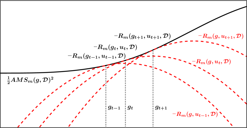
Figure 1: An illustration of the progress of a weighted classification cascade.

1.1 Related work

The functional form $b_{\mathcal{D}}(g)f\mathopen{}\mathclose{{}\left(\frac{s_{\mathcal{D}}(g)}{b_{\mathcal{D}}(g)}}\right)$ for convex $f$ is evocative of the class of discrepancy measures known as $f$-divergences (Liese and Vajda, 2006). Indeed, $b_{\mathcal{D}}(g)f\mathopen{}\mathclose{{}\left(\frac{s_{\mathcal{D}}(g)}{b_{\mathcal{D}}(g)}}\right)$ can be viewed as a generalized $f$-divergence between two unnormalized measures. Nguyen et al. (2010) and Lexa (2012) have derived algorithms analogous to those derived here for optimizing $f$-divergences.

2 HiggsML Challenge Case Study

While the algorithms of Section 1 provide simple recipes for turning any classifier that supports class weights into a training set AMS maximizer, the procedures should be coupled with effective regularization strategies to ensure adequate generalization from training error to held-out test error. In this section, we will describe the practical strategies employed by the HiggsML challenge team mymo, which incorporated two variants of weighted classification cascades into its final contest solution.

The first cascade variant used the XGBoost implementation of gradient tree boosting to learn the base classifier $g_{t}$ on each round of Algorithm 1. To curb overfitting to the training set, on each cascade round, the team computed weighted true and false positive counts on a held-out validation dataset $\mathcal{D}_{\text{val}}$ and updated the class weight parameter $u_{t}$ using $s_{\mathcal{D}_{\text{val}}}(g_{t})$ and $b_{\mathcal{D}_{\text{val}}}(g_{t})$ in lieu of $s_{\mathcal{D}}(g_{t})$ and $b_{\mathcal{D}}(g_{t})$. The cascading procedure was run until the validation set AMS failed to increase (this often occurred on the third iteration) and was then run for a small number of additional rounds (typically ten). Since XGBoost is a randomized learning algorithm, this entire cascade was rerun multiple times, and the classifiers from those cascade iterations yielding the highest validation set AMS scores were incorporated into the final solution ensemble.

The second cascade variant maintained a single persistent classifier, the complexity of which grew on each cascade round. More precisely, team mymo developed a customized XGBoost classifier that, on cascade round $t$, introduced a single new decision tree based on the gradient of the round $t$ weighted classification error in Algorithm 1. In effect, each classifier $g_{t}$ was warm-started from the prior round classifier $g_{t-1}$. For this variant, the number of cascade iterations $T$ was typically set to $500$.

The final contest solution was an ensemble of cascade procedures of each variant and several non-cascaded XGBoost, random forest, and neural network models. The non-cascade models together yielded a private leaderboard score of 3.67 (198th place on the private leaderboard). Incorporating the cascade models boosted that score to 3.72594, leaving team mymo in 31st place out of the 1785 teams in the competition. A separate post-challenge assessment by team mymo revealed that averaging the predictions of ten models, five standard XGBoost models trained without cascade weighting for $T=500$ iterations and five XGBoost models trained with the second variant of cascade weighting for $T=500$ iterations led to a private leaderboard score of 3.72. These results are evidence for the utility of cascading, and we hypothesize that additional benefits will be revealed by a more comprehensive empirical evaluation of cascade regularization strategies.

References

- [1] Claire Adam-Bourdarios, Glen Cowan, Cecile Germain, Isabelle Guyon, Balazs Kegl, and David Rousseau. Learning to discover: the higgs boson machine learning challenge. URL http://higgsml.lal.in2p3.fr/documentation/.
- Borwein and Lewis [2010] Jonathan M Borwein and Adrian S Lewis. Convex analysis and nonlinear optimization: theory and examples, volume 3. Springer, 2010.
- Cowan et al. [2011] Glen Cowan, Kyle Cranmer, Eilam Gross, and Ofer Vitells. Asymptotic formulae for likelihood-based tests of new physics. The European Physical Journal C-Particles and Fields, 71(2):1–19, 2011.
- Lange et al. [2000] Kenneth Lange, David R Hunter, and Ilsoon Yang. Optimization transfer using surrogate objective functions. Journal of computational and graphical statistics, 9(1):1–20, 2000.
- Lexa [2012] Michael A Lexa. Quantization via empirical divergence maximization. Signal Processing, IEEE Transactions on, 60(12):6408–6420, 2012.
- Liese and Vajda [2006] Friedrich Liese and Igor Vajda. On divergences and informations in statistics and information theory. Information Theory, IEEE Transactions on, 52(10):4394–4412, 2006.
- Nguyen et al. [2010] XuanLong Nguyen, Martin J Wainwright, and Michael I Jordan. Estimating divergence functionals and the likelihood ratio by convex risk minimization. Information Theory, IEEE Transactions on, 56(11):5847–5861, 2010.