Point Integral Method for Solving Poisson-type Equations on Manifolds from Point Clouds with Convergence Guarantees

Abstract

Partial differential equations (PDE) on manifolds arise in many areas, including mathematics and many applied fields. Among all kinds of PDEs, the Poisson-type equations including the standard Poisson equation and the related eigenproblem of the Laplace-Beltrami operator are of the most important. Due to the complicated geometrical structure of the manifold, it is difficult to get efficient numerical method to solve PDE on manifold. In the paper, we propose a method called point integral method (PIM) to solve the Poisson-type equations from point clouds with convergence guarantees. In PIM, the key idea is to derive the integral equations which approximates the Poisson-type equations and contains no derivatives but only the values of the unknown function. The latter makes the integral equation easy to be approximated from point cloud. In the paper, we explain the derivation of the integral equations, describe the point integral method and its implementation, and present the numerical experiments to demonstrate the convergence of PIM.

1 Introduction

Partial differential equations (PDE) on manifolds arise in many areas, including geometric flows along manifolds in geometric analysis [9], movements of particles confined to surfaces in quantum mechanics [26, 10], and distributions of physical or chemical quantities along interfaces in fluid mechanics [11], among others. It is well-known that one can extract the geometric information of the manifolds by studying the behavior of partial differential equations or differential operators on the manifolds. This observation has been exploited both in mathematics, especially geometric analysis [35], and in applied fields, including machine learning [3, 17], data analysis [25], computer vision and image processing [21], geometric processing of 3D shapes [24, 19, 23]. Among all kinds of PDEs, the Poisson equation on manifolds and the related eigenproblem of the Laplace-Beltrami operator are of the most important, and have found applications in many fields. For instance, the eigensystem of the Laplace-Beltrami operator has been used for representing data in machine learning for dimensionality reduction [2], and for representing shapes in computer vision and computer graphics for the analysis of images and 3D models [24, 23].

Different approaches are available for solving the aforementioned partial differential equations, which we call the Poisson-type equations on manifolds, including Equation (P1.a), (P2.a), (P1.b), and (P2.b), which will appear in Section 2. If a manifold is represented by a mesh with nice elements, the finite element method (FEM) is effective for solving the Poisson-type equations on it. It is well-known that bad shaped elements may increase the condition number of the linear systems in FEM and hence reduce the accuracy of the solution [28]. However, for a curved manifold, it is already very difficult to obtain a globally consistent mesh [8], let alone to generate a mesh with well-shaped elements [12, 36]. To overcome the difficulty of triangulating manifolds, implicit representation (aka, level set representation) can be used, where the differential equation is extended into the ambient space and discretized using a Euclidean grid [6, 34]. However, in the applications where the ambient dimension is high, it is very expensive to lay down a Euclidean grid and solve the equations on it.

In this paper, we propose a method to solve the above Poisson-type equations on manifolds from point clouds with convergence guarantees. Unlike a mesh or a Euclidean grid, which may be difficult to generate or may introduce extra complexity, point cloud is the simplest way of representing a manifold, which is often made ready for use in practice and whose complexity depends only on the manifold itself. The main observation is that the Poisson equations can be approximated by certain integral equations which can be easily discretized and has a faithful approximation from point clouds. More precisely, we consider the Poisson equation with Neumann boundary condition:

$$\left\{\begin{array}[]{rl}-\Delta u(\mathbf{x})=f(\mathbf{x}),&\mathbf{x}\in\mathcal{M},\\ \frac{\partial u}{\partial\mathbf{n}}(\mathbf{x})=g(\mathbf{x}),&\mathbf{x}\in\partial\mathcal{M},\end{array}\right.$$ (1.3)

where $\mathcal{M}$ is a $k$ dimensional submanifold isometrically embedded in $\mathbb{R}^{d}$. We show that its solution is well approximated by the solution of the following integral equation:

$$-\frac{1}{t}\int_{\mathcal{M}}(u(\mathbf{x})-u(\mathbf{y}))R\left(\frac{|\mathbf{x}-\mathbf{y}|^{2}}{4t}\right)\mathrm{d}\mathbf{x} =$$

$$\int_{\mathcal{M}}f(\mathbf{x})\bar{R}\left(\frac{|\mathbf{x}-\mathbf{y}|^{2}}{4t}\right)\mathrm{d}\mathbf{x} + 2\int_{\partial\mathcal{M}}g(\mathbf{x})\bar{R}\left(\frac{|\mathbf{x}-\mathbf{y}|^{2}}{4t}\right)\mathrm{d}\mathbf{x}.\quad$$ (1.4)

where the function $R(r):\mathbb{R}^{+}\rightarrow\mathbb{R}^{+}$ is either compactly supported or decays exponentially and

$$\bar{R}(r)=\int_{r}^{+\infty}R(s)\mathrm{d}s.$$ (1.5)

One choice of the function $R$ is the well-known Gaussian. As the integral equation involves no derivatives of the unknown function $u$ but only the function values, it can be easily discretized from a point cloud which samples the underlying manifold. We call this method point integral method (PIM) as it only requires the approximation of integrals from the discrete representations. It has been shown that PIM has convergence guarantees for solving the Poisson-type equations on manifolds. The readers who are interested in the convergence analysis are referred to our companion papers [29]. In this paper, we focus on describing the point integral method and its implementation, and presenting the numerical experiments to demonstrate the convergence of PIM.

Related work:  Finite Element method is one of the most widely used method to solve the Poisson equations on surfaces. It has many good features. FEM converges fast: quadratically in $L^{2}$ and linearly in $H^{1}$  [15]. FEM also works for solving the eigensystem of Laplace-Beltrami operator [31, 14, 33]. In computational aspect, for Poisson equation, the stiffness matrix obtained by FEM is symmetric, positive definite and sparse. There are lots of research on the fast solver for this kind of linear systems. Despite all these advantages, as we mentioned above, FEM requires a globally consistent mesh with well-shaped elements, which is very difficult to generate for curved manifolds.

Level set method embeds the manifolds into ambient spaces, and extends the differential equations into ambient spaces, where the discretization of the differential equations can be done using Euclidean grids of the ambient space [6]. Level set method also has other advantages. For instance, with the help of implicit function, it becomes easy to estimate the normals and the curvatures of the manifold. See the discussion in [6, 7] for more details. However, the main shortcoming of the level set method is that Euclidean grids are not intrinsic to the manifold and may introduce extra computational complexity, especially in the case where the ambient dimension is high.

There are other methods which solves PDEs on manifolds directly from point clouds. Liang and Zhao [20] and Lai et al. [18] propose the methods to locally approximate the manifold and discretize the PDE using this local approximation, and assemble them together into a global linear system for solving the PDE. Their methods are essentially FEM (level set method) but over a globally non-consistent mesh (implicit function). Although it may work very well in many empirical examples, it seems difficult to analyze the convergence behavior of their methods due to the non-consistency of the mesh or the implicit function.

The point integral method is also related to the graph Laplacian with Gaussian weights. In [3, 17, 16, 5], it is shown that the graph Laplacian with Gaussian weights converges pointwisely to the Laplace-Beltrami operator when the vertices of the graph are assumed to sample the underlying manifold. The eigensystem of the weighted graph Laplacian is shown to converge to the eigensystem of the Laplace-Beltrami operator when there is no boundary [4, 13], or there is Neumann boundary [30]. Their proofs are done by relating the Laplacian to the heat operator, and thus it is essential to use the Gaussian kernel.

Organization of the paper:  The remaining of the paper is organized as follows. In Section 2, we state the problems we want to solve. We derive the integral equations which approximate the Poisson equations with Neumann and Dirichlet boundary conditions in Section 3 and 4 respectively. The details of discretizing the integral equations and its implementations are given in Section 5. In Section 6, we briefly describe the algorithm for estimating the volume weights from point clouds. In Section 7 we present several numerical results to show the performance of our method. At last, conclusion and remarks are made in Section 8.

2 Statement of the problems

In this paper, we consider the Poisson equation on a compact $k$-dimensional submanifold $\mathcal{M}$ in $\mathbb{R}^{d}$ with two kinds of boundary conditions: the Neumann boundary condition

$$\left\{\begin{array}[]{rl}-\Delta_{\mathcal{M}}u(\mathbf{x})=f(\mathbf{x}),&\mathbf{x}\in\mathcal{M}\\ \frac{\partial u}{\partial\mathbf{n}}(\mathbf{x})=g(\mathbf{x}),&\mathbf{x}\in\partial\mathcal{M}\end{array}\right.$$ (P1.a)

and the Dirichlet boundary condition,

$$\left\{\begin{array}[]{rl}-\Delta_{\mathcal{M}}u(\mathbf{x})=f(\mathbf{x}),&\mathbf{x}\in\mathcal{M}\\ u(\mathbf{x})=g(\mathbf{x}),&\mathbf{x}\in\partial\mathcal{M}\end{array}\right.$$ (P2.a)

where $\Delta_{\mathcal{M}}$ is the Laplace-Beltrami operator on $\mathcal{M}$, and $\mathbf{n}$ is the outward normal of $\partial\mathcal{M}$. Let $g$ be the Riemannian metric tensor of $\mathcal{M}$. Given a local coordinate system $(x^{1},x^{2},\cdots,x^{k})$, the metric tensor $g$ can be represented by a matrix $(g_{ij})_{k\times k}$,

$$g_{ij}=\left<\frac{\partial}{\partial x^{i}},\frac{\partial}{\partial x^{j}}\right>,\quad i,j=1,\cdots,k.$$ (2.1)

Let $(g^{ij})_{k\times k}$ is the inverse matrix of $(g_{ij})_{k\times k}$, then it is well known that the Laplace-Beltrami operator is

$$\Delta_{\mathcal{M}}=\frac{1}{\sqrt{\det g}}\frac{\partial}{\partial x^{i}}(g^{ij}\sqrt{\det g}\frac{\partial}{\partial x^{j}})$$ (2.2)

If $\mathcal{M}$ is an open set in $\mathbb{R}^{d}$ with standard Euclidean metric, then $\Delta_{\mathcal{M}}$ becomes standard Laplace operator, i.e. $\Delta_{\mathcal{M}}=\sum_{i=1}^{d}\frac{\partial^{2}}{\partial{x^{i}}^{2}}$.

The other problem we consider is the following eigenproblem of the Laplace-Beltrami operator with the Neumann boundary

$$\left\{\begin{array}[]{rcll}-\Delta_{\mathcal{M}}u(\mathbf{x})&=&\lambda u(x),&\mathbf{x}\in\mathcal{M}\\ \frac{\partial u}{\partial\mathbf{n}}(\mathbf{x})&=&0,&\mathbf{x}\in\partial\mathcal{M}.\end{array}\right.$$ (P1.b)

or the Dirichlet boundary

$$\left\{\begin{array}[]{rcll}-\Delta_{\mathcal{M}}u(\mathbf{x})&=&\lambda u(x),&\mathbf{x}\in\mathcal{M}\\ u(\mathbf{x})&=&0,&\mathbf{x}\in\partial\mathcal{M}.\end{array}\right.$$ (P2.b)

A pair $(\lambda,u)$ solving the above equations is called an eigenvalue and the corresponding eigenfunction of the Laplace-Beltrami operator $\Delta_{\mathcal{M}}$. It is well known that the spectrum of the Laplace-Beltrami operator is discrete and all eigenvalues are nonnegative. Suppose $0=\lambda_{0}\leq\lambda_{1}\leq\lambda_{2}\cdots$ are all eigenvalues listed in the ascending order and $\phi_{0},~{}\phi_{1},~{}\phi_{2},~{}\cdots$ are their corresponding eigenfunctions. Then the problem we are interested in is how to compute these eigenvalues and the corresponding eigenfunctions from point clouds.

So far, all the problems are stated in the continuous setting. Next, we will introduce the discretization of the manifold $\mathcal{M}$. Typically, the explicit form of the submanifold $\mathcal{M}$ is not known. Instead, $\mathcal{M}$ is represented by a set of sample points $P=\{\mathbf{p}_{i}|\;i=1,\cdots,n\}$, and the boundary of $\partial\mathcal{M}$ is sampled by a subset $S=\{\mathbf{s}_{i}|\;i=1,\cdots,m\}\subset P$. In addition, we may assume the following two vectors are given. The first one is $\mathbf{V}=(V_{1},\cdots,V_{n})$ where $V_{i}$ is the volume weight of $\mathbf{p}_{i}$ on $\mathcal{M}$. The second one is $\mathbf{A}=(A_{1},\cdots,A_{m})$ where $A_{i}$ is the volume weight of $\mathbf{s}_{i}$ on $\partial\mathcal{M}$. These two vectors are used to evaluate the integrals over $\mathcal{M}$ and $\partial\mathcal{M}$. For example, for any Lipschitz function $f$ on $\mathcal{M}$ and $g$ on $\partial\mathcal{M}$, $\int_{\mathcal{M}}f(x)d\mu_{x}$ and $\int_{\partial\mathcal{M}}f(x)d\tau_{x}$ can be approximated by $\sum_{i=1}^{n}f(\mathbf{p}_{i})V_{i}$ and $\sum_{i=1}^{m}f(\mathbf{s}_{i})A_{i}$ respectively.

Remark 2.1.

We remark that if $\mathbf{V}$ and $\mathbf{A}$ are not given, they can be estimated as follows.

• If a mesh with the vertices $P$ approximating $\mathcal{M}$ is given, both weight vectors $\mathbf{V}$ and $\mathbf{A}$ can be easily estimated from the given mesh by summing up the volume of the simplices incident to the vertices. One can obtain the input data which $h$-integral approximates $\mathcal{M}$ and $\partial\mathcal{M}$ if the size of the elements in the mesh is of order $h$ and the angle between the normal space of an element and the normal space of $\mathcal{M}$ at the vertices of the element is of order $h^{1/2}$ [33]. Note that there is no requirement on the shape of the elements in the mesh.

• If the points in $P$$(S)$ are independent samples from uniform distribution on $\mathcal{M}$ ($\partial\mathcal{M}$), then $\mathbf{V}$$(\mathbf{A})$ can be taken as the constant vector $1/n$$(1/m)$. The integral of the functions on $\mathcal{M}$$(\partial\mathcal{M})$ can be estimated using Monte Carol method up to the volume of $\mathcal{M}$$(\partial\mathcal{M})$;

• Finally, following [22], one can estimate the vectors $\mathbf{V}$ and $\mathbf{A}$ by locally approximating tangent spaces of $\mathcal{M}$ and $\partial\mathcal{M}$, respectively. Specifically, for a point $p\in P$, project the samples near to $p$ in $P$ onto the approximated tangent space at $p$ and take the volume of the Voronoi cell of $p$ as its weight. In this way, one avoids constructing globally consistent meshes for $\mathcal{M}$ and $\partial\mathcal{M}$.

In the paper, we assume that the submanifold $\mathcal{M}$ and its boundary $\partial\mathcal{M}$ are well resolved by the point set $P$ and $S$ in the sense that the integral of any $C^{1}$ function on $\mathcal{M}$ and $\partial\mathcal{M}$ can be well approximated from the function values on $P$ and $S$ respectively. The issue becomes how to solve the Poisson equation on $(\mathcal{M},\partial\mathcal{M}$) from the sample points $P$ and $S$ with guaranteed accuracy.

3 The Neumann Boundary Condition

Let us consider the Poisson equation with the Neumann boundary condition given by (P1.a). Given only unstructured point sets $P$ and $S$ without mesh information, it is difficult to discretize the Laplace-Beltrami operator, which is a differential operator. Our strategy is to first approximate the Poisson equation by an integral equation which involves no differentials but only the values of the unknown function, and then discretize the integral equation, which is relatively straightforward even without mesh.

We assume that the solution of the Neumann problem (P1.a) is regular enough, at least belongs to $C^{3}(\mathcal{M})$. According to the theory of elliptic equations, this assumption could be true as long as $f$, $g$, the submanifold $\mathcal{M}$ and its boundary $\partial\mathcal{M}$ are smooth enough. Furthermore, we assume the function $R:\mathbb{R}^{+}\rightarrow\mathbb{R}^{+}$ is $C^{1}(\mathbb{R}^{+})$ and $R(r)=0$ for $\forall r>1$. Under these assumptions, we can have the following main theorem of this section.

For a parameter $t$, let

$$R_{t}(\mathbf{x},\mathbf{y})=C_{t}R\left(\frac{|\mathbf{x}-\mathbf{y}|^{2}}{4t}\right)\quad\text{and}\quad\bar{R}_{t}(\mathbf{x},\mathbf{y})=C_{t}\bar{R}\left(\frac{|\mathbf{x}-\mathbf{y}|^{2}}{4t}\right),$$

where $C_{t}$ is a normalizing factor.Recall that $\bar{R}(r)=\int_{r}^{+\infty}R(s)\mathrm{d}s$. Define the following operator for any function $u$ on $\mathcal{M}$ which makes the definition meaningful.

$$L_{t}u(\mathbf{x})=\frac{1}{t}\int_{\mathcal{M}}R_{t}(\mathbf{x},\mathbf{y})(u(\mathbf{x})-u(\mathbf{y}))d\mu_{\mathbf{y}}.$$ (3.1)

Let us call $L_{t}$ is the integral Laplace operator, which is clearly defined over $L^{2}(\mathcal{M})$.

In PIM, the approximate solution of the Neumann problem (P1.a) is obtained by solving the following integral equation with small $t$.

$$L_{t}u(\mathbf{y})=2\int_{\partial\mathcal{M}}g(\mathbf{x})\bar{R}_{t}(\mathbf{x},\mathbf{y})\mathrm{d}\mathbf{x}+\int_{\mathcal{M}}f(\mathbf{x})\bar{R}_{t}(\mathbf{x},\mathbf{y})\mathrm{d}\mathbf{x}.$$ (3.2)

Similarly, one can approximate the the eigenproblem of the Laplace-Beltrami operator with the Neumann boundary given by (P1.b) by solving the following integral equation with small $t$.

$$L_{t}u(\mathbf{y})=\lambda\int_{\mathcal{M}}u(\mathbf{x})\bar{R}_{t}(\mathbf{x},\mathbf{y})\mathrm{d}\mu_{\mathbf{x}}.\quad$$ (3.3)

Note that all the terms in (3.2) and (3.3) are in the integral form, which is ready to be discretized by the point sets $P$ and $S$, and the associated volume weights $\mathbf{V}$ and $\mathbf{A}$. See Section 5 for the discretization of the above integral equations.

Following theorem gives us an explanation that why the solution of the integral equation (3.2) could approximate the solution of the Neumann problem (P1.a).

Theorem 3.1.

Let $u(\mathbf{x})$ be the solution of the Neumann problem given by (P1.a), if $u\in C^{3}(\mathcal{M})$, then

$$\left\|-L_{t}u(\mathbf{y})+2\int_{\partial\mathcal{M}}g(\mathbf{x})\bar{R}_{t}(\mathbf{x},\mathbf{y})\mathrm{d}\mathbf{x}+\int_{\mathcal{M}}f(\mathbf{x})\bar{R}_{t}(\mathbf{x},\mathbf{y})\mathrm{d}\mathbf{x}\right\|_{L^{2}(\mathcal{M})}=O(t^{1/4}).\quad$$

Remark 3.1.

Theorem 3.1 by itself does not imply that the solution of the integral equation (3.2) respectively (3.3) converges to the solution of (P1.a) respectively (P1.b) as $t\rightarrow 0$. The convergence requires the stability of the operator $L_{t}$. The rigorous proof for the convergence of the above integral equations is out of the scope of this paper. The interested readers are referred to the companion paper [29].

In the paper, we prove Theorem 3.1 for the case where $\mathcal{M}$ is an open set of Euclidean space $\mathbb{R}^{k}$. For a general submanifold, the proof follows from the same idea but is technically more involved. The interested readers are referred to [29]. In what follows, use $\Omega$ to denote the open set $\mathcal{M}$ in $\mathbb{R}^{k}$. First, we prove a technical lemma.

Lemma 3.1.

For any function $u\in C^{3}(\Omega)$, we have

$$\frac{1}{2t}\int_{\Omega}(\mathbf{x}-\mathbf{y})\cdot\nabla u(\mathbf{x})R_{t}(\mathbf{x},\mathbf{y})\mathrm{d}\mathbf{x} = \frac{1}{2t}\int_{\Omega}(u(\mathbf{x})-u(\mathbf{y}))R_{t}(\mathbf{x},\mathbf{y})\mathrm{d}\mathbf{x}+\frac{1}{2}\int_{\Omega}\Delta u\cdot\bar{R}_{t}(\mathbf{x},\mathbf{y})\mathrm{d}\mathbf{x}$$ (3.4)

$$-\frac{1}{2}\int_{\partial\Omega}((\mathbf{x}-\mathbf{y})\otimes\mathbf{n}):\mathbf{H}_{u}(\mathbf{x})\bar{R}(\mathbf{x},\mathbf{y})\mathrm{d}\mathbf{x}+O(t^{1/2})$$

where $\mathbf{H}_{u}(\mathbf{x})$ is the Hessian matrix of $u$ at $\mathbf{x}$, $\mathbf{n}$ is the outer normal vector of $\partial\Omega$.

Proof.

The Taylor expansion of the function $u$ tells us that

$$u(\mathbf{x})-u(\mathbf{y})=(\mathbf{x}-\mathbf{y})\cdot\nabla u(\mathbf{x})-\frac{1}{2}(\mathbf{x}-\mathbf{y})^{T}\mathbf{H}_{u}(\mathbf{x})(\mathbf{x}-\mathbf{y})+O(\|\mathbf{x}-\mathbf{y}\|^{3}).$$ (3.5)

Then, we have

$$\frac{1}{2t}\int_{\Omega}(\mathbf{x}-\mathbf{y})\cdot\nabla u(\mathbf{x})R_{t}(\mathbf{x},\mathbf{y})\mathrm{d}\mathbf{x}=\frac{1}{2t}\int_{\Omega}(u(\mathbf{x})-u(\mathbf{y}))R_{t}(\mathbf{x},\mathbf{y})\mathrm{d}\mathbf{x}$$

$$+\frac{1}{4t}\int_{\Omega}(\mathbf{x}-\mathbf{y})^{T}\mathbf{H}_{u}(\mathbf{x})(\mathbf{x}-\mathbf{y})R_{t}(\mathbf{x},\mathbf{y})\mathrm{d}\mathbf{x}+O(t^{1/2}).$$ (3.6)

Here we use the fact that $\int_{\Omega}\|\mathbf{x}-\mathbf{y}\|^{n}R_{t}(\mathbf{x},\mathbf{y})\mathrm{d}\mathbf{x}=O(t^{n/2})$. Now, we turn to calculate the second term of (3).

$$\frac{1}{4t}\int_{\Omega}(\mathbf{x}-\mathbf{y})^{T}\mathbf{H}_{u}(\mathbf{x})(\mathbf{x}-\mathbf{y})R_{t}(\mathbf{x},\mathbf{y})\mathrm{d}\mathbf{x}$$ (3.7)

$$= \frac{1}{4t}\int_{\Omega}(\mathbf{x}_{i}-\mathbf{y}_{i})(\mathbf{x}_{j}-\mathbf{y}_{j})\partial_{ij}u(\mathbf{x})R_{t}(\mathbf{x},\mathbf{y})\mathrm{d}\mathbf{x}$$

$$= -\frac{1}{2}\int_{\Omega}(\mathbf{x}_{i}-\mathbf{y}_{i})\partial_{ij}u(\mathbf{x})\partial_{j}\left(\bar{R}_{t}(\mathbf{x},\mathbf{y})\right)\mathrm{d}\mathbf{x}$$

$$= \frac{1}{2}\int_{\Omega}\partial_{j}(\mathbf{x}_{i}-\mathbf{y}_{i})\partial_{ij}u(\mathbf{x})\bar{R}_{t}(\mathbf{x},\mathbf{y})\mathrm{d}\mathbf{x}+\frac{1}{2}\int_{\Omega}(\mathbf{x}_{i}-\mathbf{y}_{i})\partial_{ijj}u(\mathbf{x})\bar{R}_{t}(\mathbf{x},\mathbf{y})\mathrm{d}\mathbf{x}$$

$$-\frac{1}{2}\int_{\partial\Omega}(\mathbf{x}_{i}-\mathbf{y}_{i})\mathbf{n}_{j}\partial_{ij}u(\mathbf{x})\bar{R}_{t}(\mathbf{x},\mathbf{y})\mathrm{d}\mathbf{x}$$

$$= \frac{1}{2}\int_{\Omega}\partial_{ii}u(\mathbf{x})\bar{R}_{t}(\mathbf{x},\mathbf{y})\mathrm{d}\mathbf{x}-\frac{1}{2}\int_{\partial\Omega}(\mathbf{x}_{i}-\mathbf{y}_{i})\mathbf{n}_{j}\partial_{ij}u(\mathbf{x})\bar{R}_{t}(\mathbf{x},\mathbf{y})\mathrm{d}\mathbf{x}+O(t^{1/2})$$

$$= \frac{1}{2}\int_{\Omega}\Delta u(\mathbf{x})\bar{R}_{t}(\mathbf{x},\mathbf{y})\mathrm{d}\mathbf{x}-\frac{1}{2}\int_{\partial\Omega}((\mathbf{x}-\mathbf{y})\otimes\mathbf{n}):\mathbf{H}_{u}(\mathbf{x})\bar{R}_{t}(\mathbf{x},\mathbf{y})\mathrm{d}\mathbf{x}+O(t^{1/2}).$$

Here we used Einstein’s summation convention. In the derivation of the second equality, we use the fact that

$$\partial_{j}\bar{R}_{t}(\mathbf{x},\mathbf{y})=-\frac{1}{2t}(\mathbf{x}_{j}-\mathbf{y}_{j})R_{t}(\mathbf{x},\mathbf{y}),$$

and for the fourth equality, we use the assumption that $u\in C^{3}(\Omega)$ to bound $\partial_{ijj}u(\mathbf{x})$ and thus the second term is of the order $O(t^{1/2})$. The lemma is proved by combining (3) and (3.7). ∎

Now, we are ready to prove Theorem 3.1.

Proof.

[Theorem 3.1]

Multiplying $\bar{R}_{t}(\mathbf{x},\mathbf{y})$ on both sides of the Poisson equation, and by integral by parts, we have

$$\int_{\Omega}\Delta u\cdot\bar{R}_{t}(\mathbf{x},\mathbf{y})\mathrm{d}\mathbf{x} = -\int_{\Omega}\nabla u\cdot\nabla\bar{R}_{t}(\mathbf{x},\mathbf{y})\mathrm{d}\mathbf{x}+\int_{\partial\Omega}\frac{\partial u}{\partial\mathbf{n}}\bar{R}_{t}(\mathbf{x},\mathbf{y})\mathrm{d}\mathbf{x}$$ (3.8)

$$= \frac{1}{2t}\int_{\Omega}(\mathbf{x}-\mathbf{y})\cdot\nabla u(\mathbf{x})R_{t}(\mathbf{x},\mathbf{y})\mathrm{d}\mathbf{x}+\int_{\partial\Omega}\frac{\partial u}{\partial\mathbf{n}}\bar{R}_{t}(\mathbf{x},\mathbf{y})\mathrm{d}\mathbf{x}.$$

By Lemma 3.1, we have

$$\int_{\Omega}\Delta u\cdot\bar{R}_{t}(\mathbf{x},\mathbf{y})\mathrm{d}\mathbf{x}=\frac{1}{2t}\int_{\Omega}(u(\mathbf{x})-u(\mathbf{y}))R_{t}(\mathbf{x},\mathbf{y})\mathrm{d}\mathbf{x}+\frac{1}{2}\int_{\Omega}\Delta u\cdot\bar{R}_{t}(\mathbf{x},\mathbf{y})\mathrm{d}\mathbf{x}$$

$$+\int_{\partial\Omega}\frac{\partial u}{\partial\mathbf{n}}\bar{R}_{t}(\mathbf{x},\mathbf{y})\mathrm{d}\mathbf{x}-\frac{1}{2}\int_{\partial\Omega}((\mathbf{x}-\mathbf{y})\otimes\mathbf{n}):\mathbf{H}_{u}(\mathbf{x})\bar{R}_{t}(\mathbf{x},\mathbf{y})\mathrm{d}\mathbf{x}+O(t^{1/2}),$$

which impies that

$$\int_{\Omega}\Delta u\cdot\bar{R}_{t}(\mathbf{x},\mathbf{y})\mathrm{d}\mathbf{x} = \frac{1}{t}\int_{\Omega}(u(\mathbf{x})-u(\mathbf{y}))R_{t}(\mathbf{x},\mathbf{y})\mathrm{d}\mathbf{x}+2\int_{\partial\Omega}\frac{\partial u}{\partial\mathbf{n}}(\mathbf{x})\bar{R}_{t}(\mathbf{x},\mathbf{y})\mathrm{d}\mathbf{x}$$ (3.9)

$$-\int_{\partial\Omega}((\mathbf{x}-\mathbf{y})\otimes\mathbf{n}):\mathbf{H}_{u}(\mathbf{x})\bar{R}_{t}(\mathbf{x},\mathbf{y})\mathrm{d}\mathbf{x}+O(t^{1/2}).$$

Estimate the third term on the right hand side.

$$\int_{\Omega}\left|\int_{\partial\Omega}((\mathbf{x}-\mathbf{y})\otimes\mathbf{n}):\mathbf{H}_{u}(\mathbf{x})\bar{R}_{t}(\mathbf{x},\mathbf{y})\mathrm{d}\mathbf{x}\right|^{2}\mathrm{d}\mathbf{y}$$

$$\leq \|\mathbf{H}_{u}(\mathbf{x})\|_{\infty}\int_{\Omega}\left(\int_{\partial\Omega}\|\mathbf{x}-\mathbf{y}\|\bar{R}_{t}(\mathbf{x},\mathbf{y})\mathrm{d}\mathbf{x}\right)^{2}\mathrm{d}\mathbf{y}$$

$$\leq \|\mathbf{H}_{u}(\mathbf{x})\|_{\infty}\left\|\int_{\partial\Omega}\|\mathbf{x}-\mathbf{y}\|\bar{R}_{t}(\mathbf{x},\mathbf{y})\mathrm{d}\mathbf{x}\right\|_{\infty}\int_{\partial\Omega}\left(\int_{\Omega}\|\mathbf{x}-\mathbf{y}\|\bar{R}_{t}(\mathbf{x},\mathbf{y})\mathrm{d}\mathbf{y}\right)\mathrm{d}\mathbf{x}.$$

Notice that

$$\left\|\int_{\partial\Omega}\|\mathbf{x}-\mathbf{y}\|\bar{R}_{t}(\mathbf{x},\mathbf{y})\mathrm{d}\mathbf{x}\right\|_{\infty}=O(1)\quad\text{and}\quad\int_{\Omega}\|\mathbf{x}-\mathbf{y}\|\bar{R}_{t}(\mathbf{x},\mathbf{y})\mathrm{d}\mathbf{y}=O(t^{1/2}).$$ (3.10)

Then we have

$$\int_{\Omega}\left|\int_{\partial\Omega}((\mathbf{x}-\mathbf{y})\otimes\mathbf{n}):\mathbf{H}_{u}(\mathbf{x})\bar{R}_{t}(\mathbf{x},\mathbf{y})\mathrm{d}\mathbf{x}\right|^{2}\mathrm{d}\mathbf{y}=O(t^{1/2}).$$ (3.11)

Now if $u(\mathbf{x})$ be the solution of (P1.a), it satisfies

$$\int_{\Omega}\Delta u(\mathbf{x})\bar{R}_{t}(\mathbf{x},\mathbf{y})\mathrm{d}\mathbf{x}=-\int_{\Omega}f(\mathbf{x})\bar{R}_{t}(\mathbf{x},\mathbf{y})\mathrm{d}\mathbf{x},\quad\forall\mathbf{y}\in\Omega.$$ (3.12)

We have proved the theorem. ∎

Remark 3.2.

Theorem 3.1 also holds for those $R$ which decays exponentially, such as the Gaussian function. The proof is similar.

4 The Dirichlet boundary condition

In this section, we consider the Poisson equation with the Dirichlet boundary given by (P2.a). We bridge the difference between the Neumann boundary and the Dirichlet boundary using the so-called the Robin boundary which mixes the Neumann boundary with the Dirichlet boundary. Specifically, consider the following problem

$$\left\{\begin{array}[]{rl}-\Delta u(\mathbf{x})=f(\mathbf{x}),&\mathbf{x}\in\mathcal{M},\\ u(\mathbf{x})+\beta\frac{\partial u}{\partial\mathbf{n}}(\mathbf{x})=g(\mathbf{x}),&\mathbf{x}\in\partial\mathcal{M}.\end{array}\right.$$ (P3.a)

where $\beta>0$ is a parameter.

As there is a Neumann component in the Robin boundary, we can solve the Robin problem (P3.a) using the framework of solving Neumann problem (P1.a) in Section 3. Specifically, we approximate the Robin problem (P3.a) by the following integral equation.

$$L_{t}u(\mathbf{y})-\frac{2}{\beta}\int_{\partial\mathcal{M}}(g(\mathbf{x})-u(\mathbf{x}))\bar{R}_{t}(\mathbf{x},\mathbf{y})\mathrm{d}\tau_{\mathbf{x}}=\int_{\mathcal{M}}f(\mathbf{x})\bar{R}_{t}(\mathbf{x},\mathbf{y})\mathrm{d}\mu_{\mathbf{x}}.\quad\quad$$ (4.1)

Similarly, the corresponding eigenproblem of the Laplace-Beltrami operator with zero Robin boundary (i.e., $g=0$) can be approximated by the following integral equation.

$$L_{t}u(\mathbf{y})+\frac{2}{\beta}\int_{\partial\mathcal{M}}u(\mathbf{x})\bar{R}_{t}(\mathbf{x},\mathbf{y})\mathrm{d}\tau_{\mathbf{x}}=\lambda\int_{\mathcal{M}}u(\mathbf{x})\bar{R}_{t}(\mathbf{x},\mathbf{y})\mathrm{d}\mu_{\mathbf{x}}$$ (4.2)

Theoretically, it can be shown that the solution of (P3.a) is a good approximation of the solution of the Dirichlet problem (P2.a) when $\beta$ is small.

Theorem 4.1 ([29]).

Suppose $u$ is the solution of the Dirichlet problem (P2.a) and $u_{R,\beta}$ is the solution of the Robin problem (P3.a), then

$$\|u-u_{R,\beta}\|_{H^{1}(\mathcal{M})}\leq C\beta^{1/2}\|u\|_{H^{2}(\mathcal{M})}.$$ (4.3)

Therefore, we can approximate the Dirichlet problem (P2.a) and the corresponding eigenproblem using the integral equation (4.1) and (4.2) respectively by choosing small enough $\beta$. In a companion paper [29], it is shown that the above approximations indeed converge as $t$ goes to $0$. Note that the choice of $\beta$ depends on $t$ and has to go to $0$ as $t$ goes to $0$. Again the integral equations (4.1) and (4.2) are ready to be discretized by the input data $(P,S,\mathbf{V},\mathbf{A})$. See Section 5 for the discretization of the above integral equations.

4.1 Iterative Solver based on Augmented Lagrangian Multiplier

Notice that when $\beta$ is small, the linear system derived from the above approach becomes ill-conditioned. We now propose an iterative method based on the Augmented Lagrange method (ALM) to alleviate the dependence on the choice of $\beta$. We have not been able to show the convergence of this iterative method. However, we shall provide the theoretical evidence (see Section 4.2) as well as the empirical evidence (see Section 7) to support its convergence.

Procedure 1 ALM for Dirichlet Problem

1:  $k=0$, $w^{0}=0$.

2:  repeat

3:     Solving the following integral equation to get $v^{k}$,

$$L_{t}v^{k}(\mathbf{y}) - \frac{2}{\beta}\int_{\partial\mathcal{M}}(g(\mathbf{x})-v^{k}(\mathbf{x})+\beta w^{k}(\mathbf{x}))\bar{R}_{t}(\mathbf{x},\mathbf{y})\mathrm{d}\tau_{\mathbf{x}}\ =\int_{\mathcal{M}}f(\mathbf{x})\bar{R}_{t}(\mathbf{x},\mathbf{y})\mathrm{d}\mu_{\mathbf{x}}.$$

4:     $w^{k+1}=w^{k}+\frac{1}{\beta}(g-(v^{k}|_{\partial\mathcal{M}}))$, $k=k+1$

5:  until $\|g-(v^{k-1}|_{\partial\mathcal{M}})\|==0$

6:  $u=v^{k}$

It is well known that the Dirichlet problem can be reformulated using the following constrained variational problem:

$$\min_{v\in H^{1}(\mathcal{M})}\frac{1}{2}\int_{\mathcal{M}}|\nabla v(\mathbf{x})|^{2}\mathrm{d}\mathbf{x}+\int_{\mathcal{M}}f(\mathbf{x})v(\mathbf{x})\mathrm{d}\mathbf{x},\quad\mbox{subject to:}\;\;\;v(\mathbf{x})|_{\partial\mathcal{M}}=g(\mathbf{x}),$$ (4.4)

and the ALM method can be used to solve the above problem as follows. Recall that for a constrained optimization problem

$$\min_{x}F(x),\quad\mbox{subject to:}\quad g(x)=0,$$ (4.5)

the ALM method solves it by the following iterative process

• $x^{k}=\arg\min_{x}L(x,w^{k})$, where $L(x,w)=F(x)+<w,g(x)>+\frac{1}{2\beta}\|g(x)\|^{2}$

• $w^{k+1}=w^{k}+\frac{1}{\beta}g(x^{k})$.

In essence, the ALM method solves a constrained problem by iteratively solving a sequence of unconstrained problem. It is well known that the convergence of ALM method is robust to the choice of the parameter $\beta$.

Applying the ALM method directly to the problem (4.4), the unconstrained problem which need to be solved iteratively is

$$\min_{v} \frac{1}{2}\int_{\mathcal{M}}|\nabla v(\mathbf{x})|^{2}\mathrm{d}\mu_{\mathbf{x}}+\int_{\mathcal{M}}f(\mathbf{x})\cdot v(\mathbf{x})\mathrm{d}\mu_{\mathbf{x}}$$ (4.6)

$$+\int_{\partial\mathcal{M}}w^{k}(\mathbf{x})\cdot(g(\mathbf{x})-v(\mathbf{x}))\mathrm{d}\tau_{\mathbf{x}}+\frac{1}{2\beta}\int_{\partial\mathcal{M}}(g(\mathbf{x})-v(\mathbf{x}))^{2}\mathrm{d}\tau_{\mathbf{x}}.$$

Using the variational method, one can show that the solution to (4.6) is exactly the solution to the following Poisson equation with the Robin boundary:

$$\left\{\begin{array}[]{cl}\Delta v(\mathbf{x})=f(\mathbf{x}),&\mathbf{x}\in\mathcal{M},\\ v(\mathbf{x})+\beta\frac{\partial v}{\partial\mathbf{n}}(\mathbf{x})=g(\mathbf{x})+\beta w^{k}(\mathbf{x}),&\mathbf{x}\in\partial\mathcal{M}.\end{array}\right.$$ (4.9)

Therefore, we have derived a method to solve the Dirichlet problem (P2.a) by solving a sequence of the Robin problem in (4.9) with the iteratively updated $w^{k}$. If the iterative process converges, we obtain the correct boundary condition, i.e., $v(\mathbf{x})=g(\mathbf{x})$ for $\mathbf{x}\in\partial\mathcal{M}$. In fact, $w^{k}$ converges to $\frac{\partial v}{\partial\mathbf{n}}(\mathbf{x})$ for $\mathbf{x}\in\partial\mathcal{M}$. So, it is not necessary to choose $\beta$ small to achieve the prescribed Dirichlet boundary. Finally, we summarize the above iterative method for solving the Dirichlet problem in Procedure 1 (ALM for Dirichlet Problem).

4.2 Towards a convergence analysis of the ALM iteration

We have not been able to proved the convergence of the above ALM iteration described in Procedure 1. However, if the Robin problem (4.9) is exactly solved in each iteration, we can prove that the ALM iteration converges and hence the obtained solution converges the exact solution of the Dirichlet problem (P2.a).

Theorem 4.2.

Let $u$ be the solution of the Dirichlet problem (P2.a) and $v^{k}$ be the exact solution of (4.9) in the $k$th step. Then

$$\lim_{k\rightarrow\infty}\|u-v^{k}\|_{H^{1}(\mathcal{M})}=0.$$ (4.10)

Proof.

Let $e^{k}(\mathbf{x})=v^{k}(\mathbf{x})-u(\mathbf{x})$, then $e^{k}$ satisfies the following equation

$$\left\{\begin{array}[]{cl}\Delta e^{k}(\mathbf{x})=0,&\mathbf{x}\in\mathcal{M},\\ e^{k}(\mathbf{x})+\beta\frac{\partial e^{k}}{\partial\mathbf{n}}(\mathbf{x})=\beta\frac{\partial e^{k-1}}{\partial\mathbf{n}}(\mathbf{x}),&\mathbf{x}\in\partial\mathcal{M}.\end{array}\right.$$ (4.13)

Multiplying $e^{k}$ to both sides of the above equation and integrate by part,

$$-\int_{\mathcal{M}}|\nabla e^{k}|^{2}\mathrm{d}\mu_{\mathbf{x}}+\int_{\partial\mathcal{M}}\frac{\partial e^{k}}{\partial\mathbf{n}}(\mathbf{x})e^{k}(\mathbf{x})\mathrm{d}\tau_{\mathbf{x}}=0,$$ (4.14)

which together with the boundary condition in (4.13) gives us that

$$\int_{\mathcal{M}}|\nabla e^{k}|^{2}\mathrm{d}\mu_{\mathbf{x}}+\beta\int_{\partial\mathcal{M}}\left|\frac{\partial e^{k}}{\partial\mathbf{n}}\right|^{2}\mathrm{d}\tau_{\mathbf{x}}=\beta\int_{\partial\mathcal{M}}\frac{\partial e^{k}}{\partial\mathbf{n}}(\mathbf{x})\cdot\frac{\partial e^{k-1}}{\partial\mathbf{n}}(\mathbf{x})\mathrm{d}\tau_{\mathbf{x}}.$$ (4.15)

Using the inequality

$$\int_{\partial\mathcal{M}}\frac{\partial e^{k}}{\partial\mathbf{n}}(\mathbf{x})\cdot\frac{\partial e^{k-1}}{\partial\mathbf{n}}(\mathbf{x})\mathrm{d}\tau_{\mathbf{x}}\leq\frac{1}{2}\int_{\partial\mathcal{M}}\left|\frac{\partial e^{k}}{\partial\mathbf{n}}\right|^{2}\mathrm{d}\tau_{\mathbf{x}}+\frac{1}{2}\int_{\partial\mathcal{M}}\left|\frac{\partial e^{k-1}}{\partial\mathbf{n}}\right|^{2}\mathrm{d}\tau_{\mathbf{x}},$$ (4.16)

we obtain

$$\int_{\mathcal{M}}|\nabla e^{k}|^{2}\mathrm{d}\mu_{\mathbf{x}}+\frac{\beta}{2}\int_{\partial\mathcal{M}}\left|\frac{\partial e^{k}}{\partial\mathbf{n}}\right|^{2}\mathrm{d}\tau_{\mathbf{x}}\leq\frac{\beta}{2}\int_{\partial\mathcal{M}}\left|\frac{\partial e^{k-1}}{\partial\mathbf{n}}\right|^{2}\mathrm{d}\tau_{\mathbf{x}}.$$ (4.17)

Now, let

$$a^{k}=\int_{\partial\mathcal{M}}\left|\frac{\partial e^{k}}{\partial\mathbf{n}}\right|^{2}\mathrm{d}\tau_{\mathbf{x}},\quad k=1,2,\cdots$$ (4.18)

Since $\int_{\mathcal{M}}|\nabla e^{k}|^{2}\mathrm{d}\mu_{\mathbf{x}}\geq 0$ and $\beta>0$, we have

$$0\leq a^{k}\leq a^{k-1},\quad\forall k\in\mathbb{N}$$ (4.19)

which means that $\{a^{k}\}$ is a monotonously decreasing sequence which is bounded below by 0. Then the sequence $\{a^{k}\}$ converges which implies that

$$\lim_{k\rightarrow\infty}(a^{k-1}-a^{k})=0.$$ (4.20)

Then, let $k$ go to $\infty$ in inequality (4.17), we have

$$0\leq\lim_{k\rightarrow\infty}\int_{\mathcal{M}}|\nabla e^{k}|^{2}\mathrm{d}\mu_{\mathbf{x}}\leq\frac{\beta}{2}\lim_{k\rightarrow\infty}(a^{k-1}-a^{k})=0$$ (4.21)

which implies that

$$\lim_{k\rightarrow\infty}\int_{\mathcal{M}}|\nabla e^{k}|^{2}\mathrm{d}\mu_{\mathbf{x}}=0.$$ (4.22)

Since $e^{k}$ satisfies (4.13), we have

$$-\int_{\mathcal{M}}\nabla e^{k}\cdot\nabla\varphi\mathrm{d}\mu_{\mathbf{x}}+\int_{\partial\mathcal{M}}\frac{\partial e^{k}}{\partial\mathbf{n}}\varphi\mathrm{d}\tau_{\mathbf{x}}=0,\quad\forall\varphi\in H^{1}(\mathcal{M}).$$ (4.23)

Letting $k\rightarrow\infty$, we get

$$\lim_{k\rightarrow\infty}\int_{\partial\mathcal{M}}\frac{\partial e^{k}}{\partial\mathbf{n}}\varphi\mathrm{d}\tau_{\mathbf{x}}=0,\quad\forall\varphi\in H^{1}(\mathcal{M}).$$ (4.24)

By the boundary condition $(e^{k}+\beta\frac{\partial e^{k}}{\partial\mathbf{n}})|_{\partial\mathcal{M}}=\beta\frac{\partial e^{k-1}}{\partial\mathbf{n}}|_{\partial\mathcal{M}}$, we can derive

$$\lim_{k\rightarrow\infty}\int_{\partial\mathcal{M}}e^{k}\,\varphi\mathrm{d}\tau_{\mathbf{x}}=0,\quad\forall\varphi\in H^{1}(\mathcal{M}).$$ (4.25)

Then by the Poincare inequality, it is easy to show that

$$\lim_{k\rightarrow\infty}\int_{\mathcal{M}}|e^{k}|^{2}\mathrm{d}\mu_{\mathbf{x}}=0$$ (4.26)

∎

Remark 4.1.

Theorem 4.2 does not imply the convergence of Procedure 1. In Procedure 1, $u^{k}$ is not an exact solution of the Robin problem as is required in the above theorem. Theoretically, we can not exclude the case that the error in each iteration accumulates so that the iterative process diverges. However in the experiments we have done, Procedure 1 always converges to the right answer.

5 Discretization of the integral equations

In this section, we discretize the integral equations derived in Section 3 and Section 4 over the given input data $(P,S,\mathbf{V},\mathbf{A})$. We assemble three matrices from the input data $(P,S,\mathbf{V},\mathbf{A})$ which are used to do numerical integral.

The first matrix, denoted $\mathcal{L}$, is an $n\times n$ matrix defined as for any $\mathbf{p}_{i},\mathbf{p}_{j}\in P$

$$\mathcal{L}_{ij}=\left\{\begin{array}[]{rl}-\frac{1}{t}R_{t}({\bf p}_{i},{\bf p}_{j})V_{j}\text{~{}~{}if~{}~{}}i\neq j\\ -\sum_{i\neq j}\mathcal{L}_{ij}\text{~{}~{}if~{}~{}}i=j.\end{array}\right.$$ (5.3)

For any function $u\in C^{1}(M)$, let ${\bf u}=(u_{1},\cdots,u_{n})$ with $u_{i}=u(p_{i})$ for any $p_{i}\in P$. Then $\mathcal{L}\mathbf{u}$ is used to approximate the integral

$$\frac{1}{t}\int_{\mathcal{M}}R_{t}(\mathbf{x},\mathbf{y})(u(\mathbf{x})-u(\mathbf{y}))d\mu_{\mathbf{y}}$$ (5.4)

The matrix $\mathcal{L}$ was introduced as a discrete Laplace operator in [3].

The second matrix, denoted $\mathcal{I}$, is also an $n\times n$ matrix defined as for any $\mathbf{p}_{i},\mathbf{p}_{j}\in P$

$$\mathcal{I}_{ij}=\bar{R}_{t}({\bf p}_{i},{\bf p}_{j})V_{j}$$ (5.5)

For any function $f\in C^{1}(M)$, let ${\bf f}=(f_{1},\cdots,f_{n})$ with $f_{i}=f(\mathbf{p}_{i})$ for any $\mathbf{p}_{i}\in P$. Then $\mathcal{I}{\bf f}$ is used to approximate the integral

$$\int_{\mathcal{M}}\bar{R}_{t}(\mathbf{x},\mathbf{y})f(\mathbf{y})d\mu_{\mathbf{y}}.$$ (5.6)

The third matrix, denoted $\mathcal{B}$, is an $n\times m$ matrix defined as for any $\mathbf{p}_{i}\in P$ and any $\mathbf{s}_{j}\in S$

$$\mathcal{B}_{ij}=\bar{R}_{t}({\bf p}_{i},{\bf s}_{j})A_{j}$$ (5.7)

For any function $g\in C^{1}(\partial M)$, let ${\bf g}=(g_{1},\cdots,g_{n})$ with $g_{i}=g(\mathbf{s}_{i})$ for any $\mathbf{s}_{i}\in S$ Then $\mathcal{B}{\bf g}$ is used to approximate the integral

$$\int_{\partial\mathcal{M}}\bar{R}_{t}(\mathbf{x},\mathbf{y})g(\mathbf{y})d\tau_{\mathbf{y}}.$$ (5.8)

Now we are ready to describe the algorithms to solve the Poisson equation with different boundary conditions. As we will see, they are simple and easy to implement. The following algorithm PoissonNeumann is used to solve the Poisson equation with the Neumann boundary. The derivation of the algorithm is described in the Section 3.

Algorithm 2 PoissonNeumann($P,S,\mathbf{V},\mathbf{A},{\bf f},{\bf g},t$)

1:  Compute the matrices $\mathcal{L},\mathcal{I},\mathcal{B}$.

2:  Set ${\bf b}=2\mathcal{B}{\bf g}+\mathcal{I}{\bf f}$.

3:  Solve the linear system $\mathcal{L}{\bf u}={\bf b}$ and obtain ${\bf u}=(u_{1},\cdots,u_{n})$.

4:  Output ${\bf u}$.

The eigenvalues and the eigenfunctions of the Laplace-Beltrami operator with the Neumann boundary condition are approximated by that of the generalized eigenproblem $\mathcal{L}{\bf v}=\gamma\mathcal{I}{\bf v}$. Specifically, the $k$th smallest eigenvalue $\gamma_{k}$ and its corresponding ${\bf v}_{k}$ are used to approximate $\lambda_{k}$ and $\phi_{k}$ respectively. See Algorithm $3$ EigenNeumann.

Algorithm 3 EigenNeumann($P,S,\mathbf{V},\mathbf{A},t$)

1:  Compute the matrices $\mathcal{L},\mathcal{I}$.

2:  Solve the generalized eigenproblem $\mathcal{L}{\bf v}=\gamma\mathcal{I}{\bf v}$ and obtain the eigenvalues $0=\gamma_{0}\leq\gamma_{1}\leq\gamma_{2},\cdots$ and the corresponding eigenvectors ${\bf v}_{0},~{}{\bf v}_{1},~{}{\bf v}_{2},\cdots$

3:  Output $\gamma_{i}$ and ${\bf v}_{i}$.

For the Dirichlet problem, we approximate the solutions using those of the Robin problem with small $\beta$. The algorithms for solving the Dirichlet problem and the corresponding eigenproblems are summarized in Algorithm 4 PoissonDirichlet and Algorithm 5 EigenDirichlet, respectively. In the following algorithm, for any subset $X\subset P$, use $X$ to also denote the set of indices of the elements in $X$.

Algorithm 4 PoissonDirichlet($P,S,\mathbf{V},\mathbf{A},{\bf f},{\bf g},t,\beta$)

1:  Compute the matrices $\mathcal{L},\mathcal{I},\mathcal{B}$.

2:  Set ${\bf b}=\frac{2}{\beta}\mathcal{B}{\bf g}+\mathcal{I}{\bf f}$.

3:  Set $K=\mathcal{L}$ and modify $K(P,S)=K(P,S)+\frac{2}{\beta}\mathcal{B}$

4:  Solve the linear system $K{\bf u}={\bf b}$ and obtain ${\bf u}=(u_{1},\cdots,u_{n})$.

5:  Output ${\bf u}$.

Algorithm 5 EigenDirichlet($P,S,\mathbf{V},\mathbf{A},t,\beta$)

1:  Compute the matrices $\mathcal{L},\mathcal{I},\mathcal{B}$.

2:  Set $K=\mathcal{L}$ and modify $K(P,S)=K(P,S)+\frac{2}{\beta}\mathcal{B}$

3:  Solve the generalized eigenproblem $K{\bf v}=\gamma\mathcal{I}{\bf v}$ and obtain the eigenvalues $0<\gamma_{1}\leq\gamma_{2}\leq\gamma_{3},\cdots$ and the corresponding eigenvectors ${\bf v}_{0},~{}{\bf v}_{1},~{}{\bf v}_{2},\cdots$

4:  Output $\gamma_{i}$ and ${\bf v}_{i}$.

Note that the choice of $\beta$ in the above two algorithms has to be small to achieve a good approximation. On the other hand, it can not be too small and is theoretically at least of order $\sqrt{t}$ (see Theorem $3.3$ [29]) for ${\bf u}$ computed by the algorithm PoissonDirichlet to converge.

In all the above algorithms, there is a parameter $t$, whose choice depends on the input data, in particular, the density of $P$ and $S$. In Section 7, we will show how to empirically choose $t$ to achieve the best accuracy. For the choice of $t$ with theoretically guaranteed convergence, the readers are referred to [29].

Finally, we write down the ALM iterative algorithm for solving the Dirichlet problem given in (P2.a). Recall in this method, the Dirichlet problem is modeled as a constrained optimization problem and is solved by an ALM iterative procedure where each iteration consists of solving a Robin problem as given in (4.9). See the algorithm ALMDirichlet. The purpose of the ALM iteration is to alleviate the requirement for $\beta$ being small, which is demonstrated empirically in Section 7. We remark that we have not been able to show this ALM iterative procedure converge theoretically, although we have provided some evidence to support its convergence in Section 4.2.

Algorithm 6 ALMDirichlet($P,S,\mathbf{V},\mathbf{A},{\bf f},{\bf g},t,\beta$)

1:  Compute the matrices $\mathcal{L},\mathcal{I},\mathcal{B}$.

2:  Set ${\bf b}_{0}=\mathcal{I}{\bf f}$.

3:  Set $K=\mathcal{L}$ and modify $K(P,S)=K(P,S)+\frac{2}{\beta}\mathcal{B}$.

4:  Set $\mathbf{w}=0$.

5:  repeat

6:     Set ${\bf b}={\bf b}_{0}+2\mathcal{B}(\frac{1}{\beta}{\bf g}+\mathbf{y})$.

7:     Solve the linear system $K{\bf u}={\bf b}$ and obtain ${\bf u}=(u_{1},\cdots,u_{n})$.

8:     Modify $\mathbf{w}=\mathbf{w}+\frac{1}{\beta}({\bf g}-{\bf u}(S))$.

9:  until  $\|{\bf g}-{\bf u}(S)\|$ = 0 .

10:  Output ${\bf u}$.

6 Volume weight estimations

In this section, for the sake of completeness, we give a brief description of the approach proposed in [22] to estimate the volume weight vector $\mathbf{V}$ from the point sets $P$. Using the same approach, the weight vector $\mathbf{A}$ can be estimated from $S$. The basic idea is to construct a local patch around a sample point, from which the weight of that point is computed. The detailed algorithm is described in Algorithm $7$ EstimateWeights.

Algorithm 7 EstimateWeights($P,k,n$)

1:  for each point $p\in P$  do

2:     Find the $n$-nearest neighbors of $p$ in $P$, denoted $N_{p}$.

3:     Set $\delta=\frac{1}{|N_{p}|}\sum_{q\in N_{p}}\|p-q\|$ and $N_{\delta}=\{q\in P|\|p-q\|<\delta\}$ be the points in $P$ within $\delta$ distance to $p$.

4:     Estimate the tangent space at $p$ by a $k$-dimensional subspace $\tilde{T}_{p}$ estimated from $N_{\delta}$ using weighted least squares.

5:     Project the points in $N_{\delta}$ into $\tilde{T}_{p}$ and denote them by $\tilde{N}_{\delta}$

6:     Compute the Voronoi diagram of $\tilde{N}_{\delta}$ on $\tilde{T}_{p}$.

7:     The volume weight $V_{p}$ is estimated as the volume of the Voronoi cell.

8:  end for

Theoretically, if $\delta$ in Algorithm $7$ is fixed to be a fraction of the reach of $\mathcal{M}$, then we have the following theorem which guarantees that the integral of any Lipschitz function on $\mathcal{M}$ can be well approximated using the volume weights $V_{p}$ estimated by Algorithm $7$. A sampling $P$ of $\mathcal{M}$ is an $(\epsilon,\eta)$-sampling if for any point $x\in M$, there is a point $p\in P$, so that $|x-p|<\epsilon$ and for any two different sample points $p,q\in P$, $|p-q|>\eta$.

Theorem 6.1 ([22]).

Given an $(\epsilon,\eta)$-sampling $P$ of $\mathcal{M}$ with $\epsilon$ sufficiently small, compute the volume weight $V_{p}$ for each $p\in P$ using Algorithm $7$. Then for any Lipschitz function $f$ we have that

$$\left|\int_{\mathcal{M}}f-\sum_{p\in P}V_{p}f(p)\right|=~{}O(\epsilon+\epsilon^{3}/\eta^{2}),$$

implying that for $\eta=\Omega(\epsilon^{3/2-\xi})$ with any positive constant $\xi$, we have

$$\lim_{\epsilon\rightarrow 0}\left|\int_{\mathcal{M}}f-\sum_{p\in P}V_{p}f(p)\right|=~{}0.$$

The reach of $\mathcal{M}$ is usually unknown. In practice, $\delta$ is estimated using the average distance to the $n$-nearest neighbors as described in Algorithm $7$, which works well. If $\mathcal{M}$ has boundary, for a point $p$ near to the boundary, we take as the volume weight $V_{p}$ the volume of the Voronoi cell which is inside the Convex hull of $\tilde{N}_{\delta}$.

7 Numerical Results

In this section, we run our point integral method on several examples, mainly to explain the choice of the parameters in our algorithm, to demonstrate the convergence of our algorithm and to compare its performance with that of finite element method. The approximation error is computed in $L_{2}$: $err=\|u-u_{gt}\|/\|u_{gt}\|$ where the $L_{2}$ norm is evaluated as $\|f\|=\sqrt{\sum_{\mathbf{p}_{i}\in P}f^{2}_{i}V_{i}}$ for a function $f$ over $\mathcal{M}$ and $\|f\|=\sqrt{\sum_{{\bf s}_{i}\in S}f^{2}_{i}A_{i}}$ for a function $f$ over $\partial\mathcal{M}$.

7.1 Unit Disk

Test our algorithm on unit disk. We discretize unit disk using a Delaunay mesh with $684$ vertices shown in Figure 1(a). This mesh is generated using Triangle [27]. We obtain a sequence of refined meshes with $2610$, $10191$ and $40269$ vertices by subdividing it once, twice and three times. In each subdivision, a triangle in the mesh is split into four smaller ones using the midpoints of the edges. Note that the mesh size is reduced by half but the number of vertices roughly get quadrupled for each subdivision. Figure 1(b) shows the mesh after one subdivision. For point integral method, we remove the mesh topology and only retain the vertices as the input point set $P$. Those vertices on the boundary of the mesh are taken as the input point set $S$.

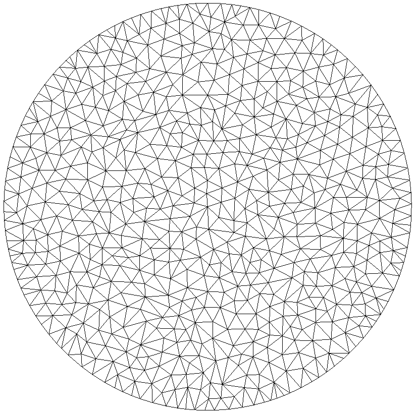
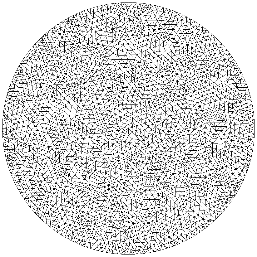
(a)	(b)

Figure 1: Discretization of unit disk. (a) A triangle mesh of unit disk with $684$ vertices. (b) The mesh with $2610$ vertices obtained by subdividing the triangle mesh in (a) where each triangle is subdivided into four using the midpoints of the edges.

Choice of Parameters:  Our algorithm has two parameters $t$ and $\beta$. Here we show how the approximation error changes with different choices of $t$ and $\beta$. Set the boundary condition (both Neumann and Dirichlet) as that of the function $u_{gt}=\cos 2\pi r$ with $r=\sqrt{x^{2}+y^{2}}$ and see how accurate our algorithm can recover this function.

Figure 2 shows the plot of the approximation error $\|u-u_{gt}\|/\|u_{gt}\|$ as a function of the parameter $\sqrt{t}$. The approximating solution $u$ is computed by Algorithm $2$ for the Neumann boundary and by Algorithm $6$ for the Dirichlet boundary. In Algorithm $6$, set $\beta=1$ and the solution is obtained after $100$ iterations. Given a sampling $P$ on $\mathcal{M}$, let $\delta_{i}$ be the average distance from $p_{i}\in P$ to its $10$ nearest neighbors in $P$ and $\delta$ is the average of $\delta_{i}$ over all points $p_{i}\in P$. We observe, from the plots in Figure 2, that the optimal parameter $\sqrt{t}$ which produces the smallest approximation error remains $0.5\delta$ for the Neumann boundary and $0.75\delta$ for the Dirichlet boundary across the above sequence of refined samplings. This means only a fixed number of samples are empirically needed in the neighborhood of size $\sqrt{t}$ for PIM to converge. Such choice of parameter $t$ leads to a better empirical convergence rate than what is predicted in [29]. The theoretical analysis for PIM in the paper [29] shows that the convergence of PIM requires more and more samples in the neighborhood of size $\sqrt{t}$ as $t$ decreases, and in fact requires infinitely many in the limit of $t$ going to $0$. As we will see below, PIM empirically converges at least linearly in mesh size, while our analysis in [29] shows that the convergence rate is one fifth root of mesh size. This phenomenon is also observed on 3D domain, as we will show in Section 7.2. This suggests that there may be rooms to improve our analysis on the convergence rate.

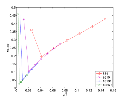
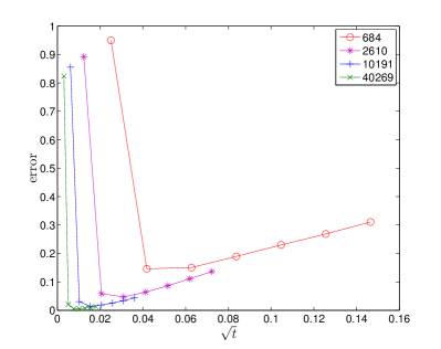
(a)	(b)

Figure 2: Approximation error vs. the parameter $t$ on unit disk: (a) Neumann boundary; (b) Dirichlet boundary

To see the choice of the parameter $\beta$, we fix the parameter $\sqrt{t}=0.75\delta$. we first show how the choice of $\beta$ affects Algorithm $4$. Figure 3 shows the approximation errors for the solution computed by Algorithm $4$ using different $\beta$ over the above sequence of refined samplings. As we can see, the effect of $\beta$ is similar across different samplings: the approximation errors remain small for $\beta$ in the interval $[10^{-6},10^{-3}]$ but increases significantly as $\beta$ increases from $10^{-3}$ or decreases from $10^{-6}$. This phenomenon fits the theory of PIM [29] well: The smaller the $\beta$ is, the smaller the approximation error is; and on the other hand, if $\beta$ is chosen too small, the linear system becomes numerically unstable and the approximation error increases. For a technical reason, our analysis in [29] also requires that $\beta$ and $\sqrt{t}$ are of the same order. However, it seems not necessary in our experiments, which means we may improve the analysis to remove this extra requirement. In the following experiments, we fix $\beta=10^{-4}$ in Algorithm $4$.

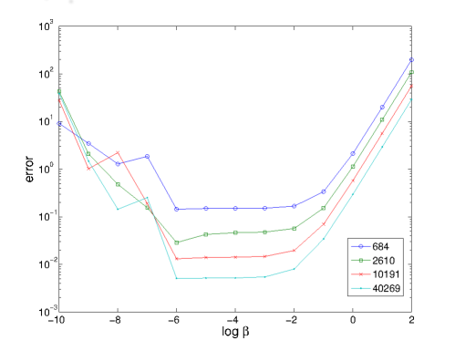
Figure 3: Approximation error vs. parameter $\beta$ by Algorithm $4$ on unit disk.

Next we show how the choice of $\beta$ affects Algorithm $6$, which employs the approach of augmented Lagrangian multiplier. We run the algorithm over the sampling with $2610$ points. Recall when the ALM iteration converges, the obtained solution should satisfy the specified boundary condition. Assume $v^{k}$ is the solution obtained after $k$th iteration. Figure 4(a) shows the approximation error $\|v^{k}|_{\partial\mathcal{M}}-g\|/\|g\|$ on the boundary. As we can see, the smaller the parameter $\beta$ is, the faster the solution $v^{k}$ converges on the boundary. However the algorithm diverges if $\beta$ is too small (less than $5\times 10^{-6}$). Nevertheless, the solution converges on the boundary over a large range of $\beta$. Figure 4(b) shows the approximation errors $\|u-u_{gt}\|/\|u_{gt}\|$ after $100$ iterations. As we can see, although the algorithm converges at the different speeds for the different $\beta$, the difference in the final approximation errors is small across the different but reasonable choices of $\beta$. Thus Algorithm 6 which employs ALM iteration is not sensitive to the choice of $\beta$ and works over a large range of $\beta$.

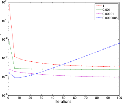
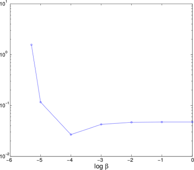
(a)	(b)

Figure 4: Choice of parameter $\beta$: (a) Convergence of $v^{k}$ on the boundary under different $\beta$; (b) Approximation error vs. parameter $\beta$.

Convergence for the Poisson Equation:  We fix $\sqrt{t}=0.75\delta$ and $\beta=10^{-4}$. We show the convergence of Algorithm 2 and Algorithm 4 for the Neumann boundary and the Dirichlet boundary respectively, and also compare them to the results of FEM. In FEM, we use linear elements. Table 1 shows the approximation error for recovering the function $\cos 2\pi r$ over a sequence of refined meshes or samplings. As we can see, FEM has the quadratic convergence rate for both the Neumann boundary and the Dirichlet boundary, which coincides with the theory of FEM. PIM converges in the linear order $h$ for the Neumann boundary and in the order $h^{3/2}$ for the Dirichlet boundary, where $h$ is referred to mesh size. This convergence rate is much faster than the order $h^{1/5}$ predicted by our analysis of PIM in [29].

$|V|$	684	2610	10191	40296
Neumann Boundary
FEM	0.0212	0.0056	0.0014	0.00036
PIM	0.1947	0.1043	0.0513	0.0249
Dirichlet Boundary
FEM	0.0310	0.0079	0.0020	0.0005
PIM	0.1500	0.0428	0.0140	0.0052

Table 1: Convergence for recovering the function $\cos 2\pi r$. The solution is computed using Algorithm 2 for Neumann boundary and Algorithm 4 for Dirichlet boundary.

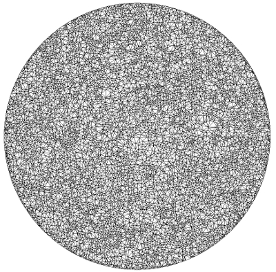
Figure 5: A triangle mesh of unit disk.

However, although FEM has a better convergence rate, it is sensitive to the quality of the mesh. Figure 5 shows a Delaunay triangle mesh with $10000$ vertices randomly sampled on unit disk. The condition number of the stiff matrix of FEM reaches $10^{20}$. Table 2 shows the approximation errors for recovering the function $\cos 2\pi r$ and the function $x^{2}-y^{2}$. As we can see, FEM is not stable and may produce a solution with no accuracy. However, PIM always produces a solution with reasonable accuracy.

	Neumann Boundary	Dirichlet Boundary
FEM	0.0026	2.0218
PIM	0.0600	0.0673
$\cos 2\pi r$
FEM	1.2003	5.0321
PIM	0.0610	0.0081
$x^{2}-y^{2}$

Table 2: The approximation errors of FEM and PIM in solving the Poisson Equations over the mesh shown in Figure 5

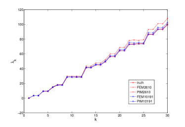
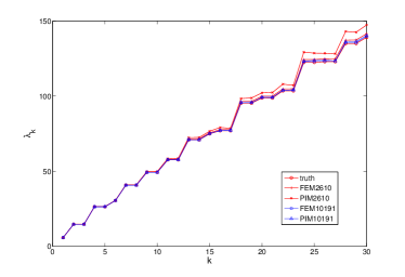
(a)	(b)

Figure 6: The eigenvalues of unit disk estimated by FEM and PIM over the meshes or the samplings with 2610 points and 10191 points. (a) Neumann eigenvalues; (b) Dirichlet eigenvalues

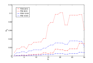
(a)	(b)

Figure 7: The approximation errors of the eigenfunctions of unit disk estimated using FEM (PIM) over the meshes (samplings) with 2610 points and 10191 points. (a) Neumann boundary; (b) Dirichlet boundary.

Eigensystem:  We compute the eigensystem of Laplacian using Algorithm 3 for the problem (P1.b) with the homogeneous Neumann boundary and Algorithm 5 for the problem (P2.b) with the homogeneous Dirichlet boundary. Again we fix $\sqrt{t}=0.75\delta$ and $\beta=10^{-4}$.

Figure 6 shows the first $30$ eigenvalues computed using PIM (FEM) over the sampling (mesh) with 2610 points and 10191 points. Both methods give a good estimation for the eigenvalues. Figure 7 shows the approximation error of the first 30 eigenfunctions, where the approximation error is computed as the angle between the eigenspaces of ground truth and the eigenspaces estimated by PIM or FEM. Let $U$ and $V$ be the two subspaces in $\mathbb{R}^{n}$. The angle between $U$ and $V$ is defined as

$$\cos\angle U,V=\min_{x\in U,|x|=1}\max_{y\in V,|y|=1}x\cdot y.$$ (7.1)

It is well-known that when two distinct eigenvalues of a matrix are close to each other, their eigenvectors computed numerically can be switched.Thus, when we estimate the approximation error of the eigenfunctions, we merge the eigenspaces of two eigenvalues close to each other. In Figure 7 (a), we merge the eigenspace of the 9th (or 10th) eigenvalue with that of the 11th eigenvalue, and the eigenspace of the 22nd (or 23rd) eigenvalue with that of the 24the eigenvalue. In Figure 7 (a), we merge the eigenspace of the 24th (or 25th) eigenvalue and that of the 26 eigenvalue.

Table 3 and Table 4 shows the convergence of the 6th eigenvalue and the corresponding eigenfunction computed using FEM and PIM. The approximation error of the ith eigenvalue is estimated as $|\lambda_{i}-\lambda_{i}^{gt}|$ where $\lambda_{i}^{gt}$ is the ground truth and $\lambda_{i}$ is the numerical estimation. The approximation error of the eigenfunction is estimated as the angle between two subspaces.

$|V|$	684	2610	10191	40296
Eigenvalue
FEM	0.1164	0.0371	0.0168	0.0116
PIM	0.8244	0.2570	0.0555	0.0212
Eigenfunction
FEM	0.0026	0.0009	0.0008	0.0008
PIM	0.0332	0.0193	0.0100	0.0052

Table 3: Convergence of the Neumann Eigensystem of unit disk.

$|V|$	684	2610	10191	40296
Eigenvalue
FEM	0.0126	0.0062	0.0045	0.0041
PIM	0.3228	0.1778	0.1115	0.0762
Eigenfunction
FEM	0.0051	0.0017	0.0014	0.0014
PIM	0.0313	0.0172	0.0079	0.0034

Table 4: Convergence of the Dirichlet Eigensystem of unit disk.

7.2 Unit Ball

Now test PIM on unit ball. The main purpose of this set of experiments is to see how PIM performs on 3D domains and what are the good ranges of the parameters for 3D domains. We discretize unit ball using 3D mesh generation package provided by CGAL [32] which is state of the art in mesh generation and uses the approach of Delaunay refinement and CVT-type of optimization for improving the mesh quality. We obtain a sequence of four refined meshes where the mesh size of a mesh is reduced roughly by half from the previous mesh. The number of vertices of the meshes are $546$, $3481$, $25606$ and $195725$. Figure 8(a) and (b) shows the mesh with $546$ and $25606$ vertices respectively. Similarly, for PIM, we remove the mesh topology and only retain the vertices as the input point set $P$. Those vertices on the boundary of the mesh are taken as the input point set $S$.

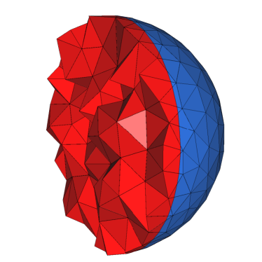
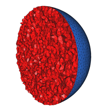
(a)	(b)

Figure 8: Discretization of unit ball using tetrahedron mesh. (a) a mesh with 546 vertices, (b) a mesh with 25606 vertices.

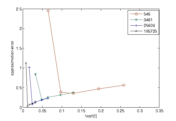
(a)	(b)

Figure 9: Approximation error vs. parameter $t$ on unit ball: (a) the Neumann boundary; (b) the Dirichlet boundary.

Choice of Parameters:  What is good choice of $\beta$ is clear from the previous experiments on unit disk. In fact, we observe the same effect of the parameter $\beta$ over the domain of unit ball, and thus we fix $\beta=10^{-4}$ for the remaining experiments. Similar to the disk case, we set the boundary condition (Neumann and Dirichlet) as that of the function $u_{gt}=\cos 2\pi r$ with $r=\sqrt{x^{2}+y^{2}+z^{2}}$ and see how accurate our algorithm can recover this function.

Figure 9 shows the plot of the approximation errors $\|u-u_{gt}\|/\|u_{gt}\|$ as a function of the parameter $\sqrt{t}$. The approximating solution $u$ is computed by Algorithm $2$ for the Neumann boundary and by Algorithm $4$ for the Dirichlet boundary. Given a sampling $P$ on $\mathcal{M}$, let $\delta_{i}$ be the average distance from $p_{i}\in P$ to its $15$ nearest neighbors in $P$ and $\delta$ is the average of $\delta_{i}$ over all points $p_{i}\in P$. From the above plot, we observe that the best parameter $\sqrt{t}$ is $0.375\delta$ for Neumann boundary and $0.75\delta$ for Dirichlet boundary. Similar to the disk case, such optimal choice of $t$ leads to much better empirical results than what is predicted in [29].

Convergence for the Poisson Equation:  We fix $\sqrt{t}=0.375\delta$ for the Neumann boundary, and $\sqrt{t}=0.75\delta$ and $\beta=10^{-4}$ for the Dirichlet boundary. We show the convergence of PIM and also compare it to FEM. In FEM, we again use linear elements. Table 1 shows the approximation errors for recovering the function $\cos 2\pi r$. As we can see, FEM has the quadratic convergence rate for both Neumann boundary and Dirichlet boundary. PIM converges in the linear order of $h$ for Neumann boundary and in the order of $h^{3/2}$ for Dirichlet boundary, where $h$ is referred to mesh size. This convergence rate is much faster than the order $h^{1/5}$ given by the analysis in [29].

$|V|$	546	3481	25606	195725
Neumann Boundary
FEM	0.2245	0.0572	0.0143	0.0036
PIM	0.3864	0.1978	0.0845	0.0293
Dirichlet Boundary
FEM	0.3896	0.0878	0.0201	0.0049
PIM	0.7572	0.2881	0.0952	0.0256

Table 5: Convergence for recovering the function $\cos 2\pi r$. The solution is computed using Algorithm 2 for Neumann boundary and Algorithm 4 for Dirichlet boundary.

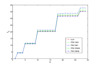
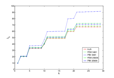
(a)	(b)

Figure 10: The eigenvalues of unit ball estimated by FEM and PIM over the meshes (samplings) with 3481 points and 25606 points. (a) Neumann eigenvalues; (b) Dirichlet eigenvalues

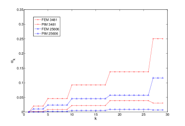
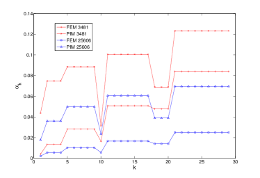
(a)	(b)

Figure 11: The approximation errors of the eigenfunctions for unit ball estimated using FEM (PIM) over the meshes (samplings) with 3481 points and 25606 points. (a) Neumann eigenfunctions; (b) Dirichlet eigenfunctions

Eigensystem:  We compute the eigensystem of Laplacian using Algorithm 3 EigenNeumann for the problem (P1.b) and Algorithm 5 EigenDirichlet for the problem (P2.b). We choose the parameters as before. Figure 10 shows the first $30$ eigenvalues computed using PIM (FEM) over the sampling (mesh) with 3481 points and 25606 points. Both methods give a good estimation for the eigenvalues. Figure 11 shows the approximation error of the first 30 eigenfunctions, where the approximation error is computed as before, i.e., the angle between the eigenspaces of ground truth and the eigenspaces estimated by PIM or FEM (see Equation (7.1)).

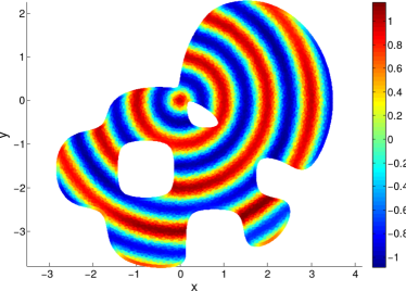
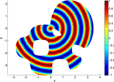
(a)	(b)

Figure 12: The function $u_{gt}=\cos 2\pi r$ recovered by PIM for Lake from a point cloud with 64131 points: (a) Neumann boundary; (b) Dirichlet boundary

7.3 An irregular Domain on Plane

We also test PIM over an irregular domain: a planar domain with two holes, which we call Lake as it looks like a lake with two islands. Again, we set the boundary condition (both Neumann and Dirichlet) as that of the function $u_{gt}=\cos 2\pi r$ with $r=\sqrt{x^{2}+y^{2}}$ and see how accurate our algorithm can recover this function. Based on the previous experiments on unit disk, we fix the parameter $\sqrt{t}=0.75\delta$ and $\beta=10^{-4}$. Figure 12 shows the functions recovered by PIM. The approximation errors of the solutions are listed in Table 6. As we can see, PIM converges in the linear order for the problem with the Neumann boundary and in the order of $h^{3/2}$ for the problem with the Dirichlet boundary. In addition, the solution for the Neumann boundary has bigger approximation errors than that for the Dirichlet boundary.

$|V|$	942	3745	16034	64131
Neumann	4.4595	1.8360	0.5842	0.3029
Dirichlet	0.3030	0.0907	0.0247	0.0081

Table 6: Convergence of PIM in solving the Poisson Equations over Lake

The ground truth of the eigenvalues and the eigenfunctions of Lake can not be expressed in an explicit way. Thus we compare the results of PIM with that of FEM. Figure 13 shows the first 30 eigenvalues of Lake estimated by PIM and FEM. Both methods give a consistent estimation of the eigenvalues of Lake. Figure 14 shows the 10th eigenfunction of Lake estimated by PIM from a point cloud with 64131 points. Table 7 shows the relative $L^{2}$ errors $\|u_{PIM}-u_{FEM}\|/\|u_{FEM}\|$ of the 10th eigenfunction estimated from different point clouds or meshes. As we can see, the relative errors decrease as the sample points increases for both boundary conditions.

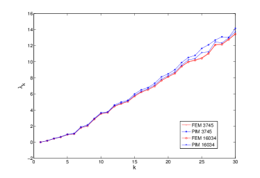
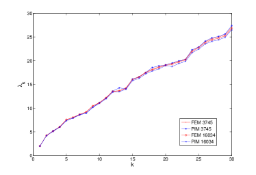
(a)	(b)

Figure 13: The eigenvalues of Lake estimated by PIM and FEM with 3745 points and 16034 points: (a) Neumann problem; (b) Dirichlet problem

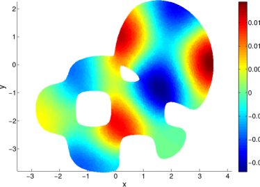
(a)	(b)

Figure 14: The 10th eigenfunction of Lake estimated by PIM from a point cloud with 64131 points: (a) Neumann problem; (b) Dirichlet problem

Number of points	942	3745	16034	64131
Neumann Boundary	0.0336	0.0124	0.0046	0.0022
Dirichlet Boundary	0.0893	0.0329	0.0088	0.0033

Table 7: The relative $L^{2}$ errors $\|u_{PIM}-u_{FEM}\|/\|u_{FEM}\|$ of the 10th eigenfunction of Lake.

7.4 General Submanifolds

In this subsection, we apply PIM to solve the Poisson equations on a few examples of general submanifolds. In the following experiments, we fix $\sqrt{t}=0.75\delta$ and $\beta=10^{-4}$.

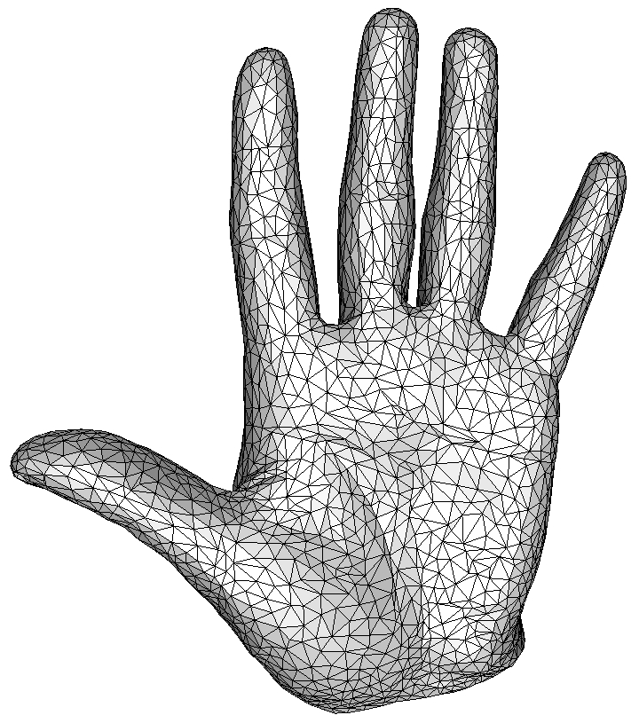
(a)	(b)

Figure 15: Lefthand (a) the original model; (b) the mesh with 3147 points

The first example is a model (Lefthand) of the left hand of a human obtained by 3D scanning. The original model is a triangle mesh with $193467$ vertices, as shown in Figure 15(a). We use Meshlib [1] to simplify the mesh to obtain the triangle meshes with $50205$, $12561$ and $3147$ vertices, over which FEM is applied to solve the Poisson equation. Figure 15(b) shows the mesh with $3147$ vertices. For PIM, the vertices of the meshes are taken as the input point sets $P$, and those on the boundary are taken as the input point sets $S$. As there is no analytic solution of the Poisson equation for a general manifold, we compare the solutions from FEM and PIM to each other, and show that they are consistent to each other. We solve over the model Lefthand the following Neumann problem

$$\left\{\begin{array}[]{rl}-\Delta u(\mathbf{x})=|\mathbf{x}|^{2},&\mathbf{x}\in\mathcal{M},\\ \frac{\partial u}{\partial\mathbf{n}}(\mathbf{x})=1,&\mathbf{x}\in\partial\mathcal{M},\end{array}\right.$$ (7.4)

and the following Dirichlet problem

$$\left\{\begin{array}[]{rl}-\Delta u(\mathbf{x})=|\mathbf{x}|^{2},&\mathbf{x}\in\mathcal{M},\\ u(\mathbf{x})=1,&\mathbf{x}\in\partial\mathcal{M}.\end{array}\right.$$ (7.7)

Figure 16 shows the solutions computed by point integral method over the point set with $193467$ points. Table 8 shows the approximation errors computed as $\|u_{PIM}-u_{FEM}\|/\|u_{FEM}\|$, where $u_{PIM}$ and $u_{FEM}$ are the solutions computed by PIM and FEM respectively. The error decreases as the number of points increases, which shows both solutions from PIM and FEM are consistent.

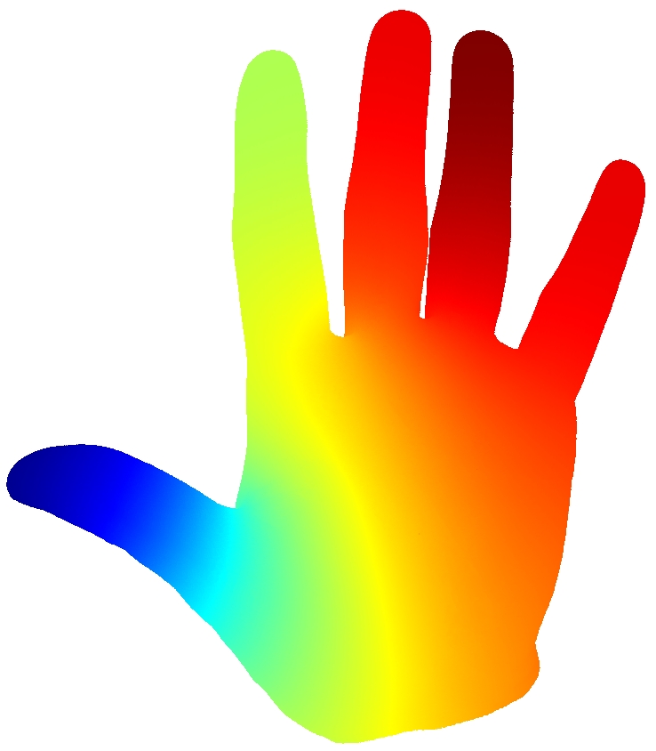
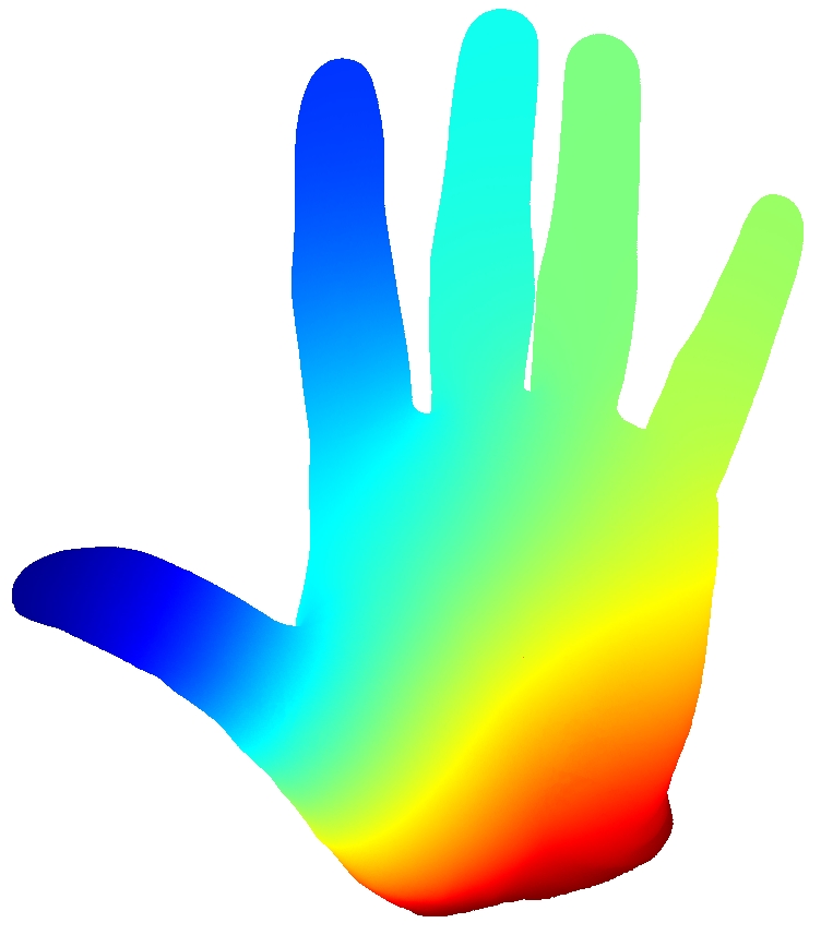
(a)	(b)

Figure 16: (a) Neumann problem (7.4); (b) Dirichlet problem (7.7)

$|V|$	3147	12561	50205	193467
Neumann	0.5944	0.0687	0.0594	0.0035
Dirichlet	0.7109	0.0259	0.0229	0.0067

Table 8: The approximation errors $\|u_{PIM}-u_{FEM}\|/\|u_{FEM}\|$ where $u_{PIM}$ and $u_{FEM}$ are the solutions of the Poisson equations (7.4) and (7.7) computed by PIM and FEM respectively.

Figure 17 shows the first $30$ eigenvalues of Lefthand using FEM over the mesh of $193467$ vertices and using PIM over the samplings with different number of points. As we can see, PIM can accurately estimate the eigenvalues of the Laplace-Beltrami operator with both the Neumann boundary and the Dirichlet boundary. Finally, Figure 18 shows the 10th eigenfunction estimated by PIM over various models.

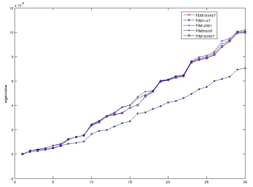
(a)	(b)

Figure 17: (a) Neumann problem; (b) Dirichlet problem

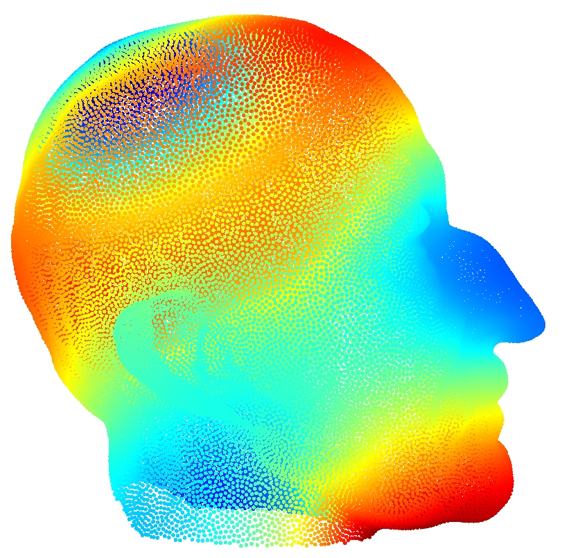
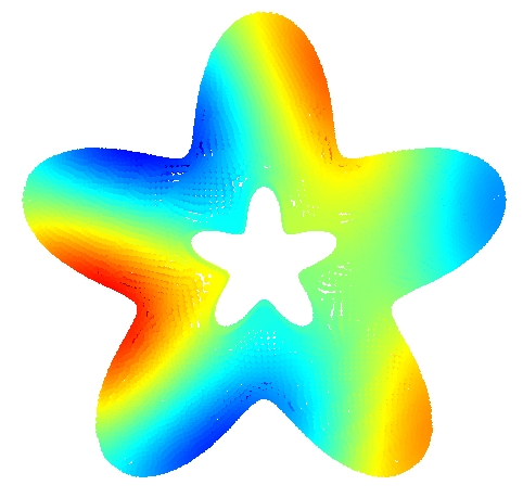
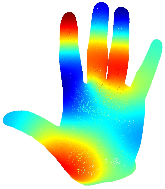
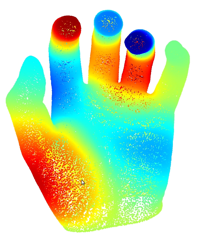
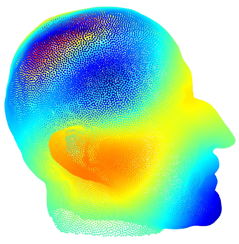
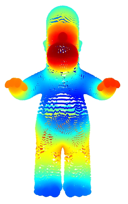
Figure 18: The 10th eigenfunction: Neumann boundary in the first row and Dirichlet boundary in the second row. Two models in the rightmost column have no boundary.

8 Conclusion

We have described the point integral method for solving the standard Poisson equation on manifolds and the eigensystem of the Laplace-Beltrami operator from point clouds, and presented a few numerical examples, which not only demonstrate the convergence of PIM in solving the Poisson-type equations, but also reveal the right choices of the parameters $t$ and $\beta$ used in PIM. In addition, the numerical experiments show PIM has a faster empirical convergence rate than what is predicted by the analysis in [29], which suggests that the analysis may be improved. We are also considering to generalize PIM to solve other PDEs on manifolds.

Acknowledgments. This research was partial supported by NSFC Grant (11201257 to Z.S., 11371220 to Z.S. and J.S. and 11271011 to J.S.), and National Basic Research Program of China (973 Program 2012CB825500 to J.S.).

References

- [1] MeshLab. http://meshlab.sourceforge.net/.
- [2] M. Belkin and P. Niyogi. Laplacian eigenmaps for dimensionality reduction and data representation. Neural Computation, 15(6):1373–1396, 2003.
- [3] M. Belkin and P. Niyogi. Towards a theoretical foundation for laplacian-based manifold methods. In COLT, pages 486–500, 2005.
- [4] M. Belkin and P. Niyogi. Convergence of laplacian eigenmaps. preprint, short version NIPS 2008, 2008.
- [5] M. Belkin, J. Sun, and Y. Wang. Constructing laplace operator from point clouds in rd. In SODA ’09: Proceedings of the Nineteenth Annual ACM -SIAM Symposium on Discrete Algorithms, pages 1031–1040, Philadelphia, PA, USA, 2009. Society for Industrial and Applied Mathematics.
- [6] M. Bertalmio, L.-T. Cheng, S. Osher, and G. Sapiro. Variational problems and partial differential equations on implicit surfaces. Journal of Computational Physics, 174(2):759 – 780, 2001.
- [7] M. Bertalmio, F. Memoli, L.-T. Cheng, G. Sapiro, and S. Osher. Variational problems and partial differential equations on implicit surfaces: Bye bye triangulated surfaces? In Geometric Level Set Methods in Imaging, Vision, and Graphics, pages 381–397. Springer New York, 2003.
- [8] J.-D. Boissonnat, R. Dyer, and A. Ghosh. Stability of delaunay-type structures for manifolds: [extended abstract]. In T. K. Dey and S. Whitesides, editors, Symposium on Computational Geometry, pages 229–238. ACM, 2012.
- [9] H.-D. Cao and S.-T. Yau. Geometric flows, volume 12 of Surveys in Differential Geometry. International Press of Boston, Inc., 2007.
- [10] R. C. T. da Costa. Quantum mechanics of a constrained particle. PHYSICAL REVIEW A, 25(6), April 1981.
- [11] R. Defay and I. Priogine. Surface Tension and Adsorption. John Wiley & Sons, New York, 1966.
- [12] T. K. Dey. Curve and Surface Reconstruction: Algorithms with Mathematical Analysis (Cambridge Monographs on Applied and Computational Mathematics). Cambridge University Press, New York, NY, USA, 2006.
- [13] T. K. Dey, P. Ranjan, and Y. Wang. Convergence, stability, and discrete approximation of laplace spectra. In Proceedings of the Twenty-First Annual ACM-SIAM Symposium on Discrete Algorithms, SODA ’10, pages 650–663, Philadelphia, PA, USA, 2010. Society for Industrial and Applied Mathematics.
- [14] J. Dodziuk and V. K. Patodi. Riemannian structures and triangulations of manifolds. Journal of Indian Math. Soc., 40:1–52, 1976.
- [15] G. Dziuk. Finite elements for the beltrami operator on arbitrary surfaces. In S. Hildebrandt and R. Leis, editors, Partial differential equations and calculus of variations, volume 1357 of Lecture Notes in Mathematics, pages 142–155. Springer, 1988.
- [16] M. Hein, J.-Y. Audibert, and U. von Luxburg. From graphs to manifolds - weak and strong pointwise consistency of graph laplacians. In Proceedings of the 18th Annual Conference on Learning Theory, COLT’05, pages 470–485, Berlin, Heidelberg, 2005. Springer-Verlag.
- [17] S. Lafon. Diffusion Maps and Geodesic Harmonics. PhD thesis, 2004.
- [18] R. Lai, J. Liang, and H. Zhao. A local mesh method for solving pdes on point clouds. Inverse Problem and Imaging, to appear.
- [19] B. Levy. Laplace-beltrami eigenfunctions towards an algorithm that ”understands” geometry. In Shape Modeling and Applications, 2006. SMI 2006. IEEE International Conference on, pages 13–13, June 2006.
- [20] J. Liang and H. Zhao. Solving partial differential equations on point clouds. SIAM Journal of Scientific Computing, 35:1461–1486, 2013.
- [21] T. Lindeberg. Scale selection properties of generalized scale-space interest point detectors. Journal of Mathematical Imaging and Vision, 46(2):177–210, 2013.
- [22] C. Luo, J. Sun, and Y. Wang. Integral estimation from point cloud in d-dimensional space: a geometric view. In Symposium on Computational Geometry, pages 116–124, 2009.
- [23] M. Ovsjanikov, J. Sun, and L. J. Guibas. Global intrinsic symmetries of shapes. Comput. Graph. Forum, 27(5):1341–1348, 2008.
- [24] M. Reuter, F.-E. Wolter, and N. Peinecke. Laplace-beltrami spectra as ”shape-dna” of surfaces and solids. Computer-Aided Design, 38(4):342–366, 2006.
- [25] N. Saito. Data analysis and representation on a general domain using eigenfunctions of laplacian. Applied and Computational Harmonic Analysis, 25(1):68 – 97, 2008.
- [26] P. Schuster and R. Jaffe. Quantum mechanics on manifolds embedded in euclidean space. Annals of Physics, 307(1):132 – 143, 2003.
- [27] J. R. Shewchuk. Triangle: Engineering a 2D Quality Mesh Generator and Delaunay Triangulator. In M. C. Lin and D. Manocha, editors, Applied Computational Geometry: Towards Geometric Engineering, volume 1148 of Lecture Notes in Computer Science, pages 203–222. Springer-Verlag, May 1996. From the First ACM Workshop on Applied Computational Geometry.
- [28] J. R. Shewchuk. What is a good linear finite element? - interpolation, conditioning, anisotropy, and quality measures. Technical report, In Proc. of the 11th International Meshing Roundtable, 2002.
- [29] Z. Shi and J. Sun. Convergence of the laplace-beltrami operator from point clouds. arXiv:1403.2141.
- [30] A. Singer and H. tieng Wu. Spectral convergence of the connection laplacian from random samples. arXiv:1306.1587.
- [31] G. Strang and G. J. Fix. An analysis of the finite element method. Prentice-Hall, 1973.
- [32] The CGAL Project. CGAL User and Reference Manual. CGAL Editorial Board, 4.4 edition, 2014.
- [33] M. Wardetzky. Discrete Differential Operators on Polyhedral Surfaces - Convergence and Approximation. PhD thesis, 2006.
- [34] J.-J. Xu and H.-K. Zhao. An eulerian formulation for solving partial differential equations along a moving interface. Journal of Scientific Computing, 19(1-3):573–594, 2003.
- [35] S.-T. Yau. The role of partial differential equations in differential geometry. In Proceedings of the International Congress of Mathematicians (Helsinki 1978), pages 237–250. Acad. Sci. Fennica, Helsinki, 1980.
- [36] H.-K. Zhao, S. Osher, and R. Fedkiw. Fast surface reconstruction using the level set method. In Proceedings of the IEEE Workshop on Variational and Level Set Methods (VLSM’01), VLSM ’01, pages 194–, Washington, DC, USA, 2001. IEEE Computer Society.