Large-scale randomized-coordinate descent methods with non-separable linear constraints

Abstract

We develop randomized block coordinate descent (CD) methods for linearly constrained convex optimization. Unlike other large-scale CD methods, we do not assume the constraints to be separable, but allow them be coupled linearly. To our knowledge, ours is the first CD method that allows linear coupling constraints, without making the global iteration complexity have an exponential dependence on the number of constraints. We present algorithms and theoretical analysis for four key (convex) scenarios: (i) smooth; (ii) smooth + separable nonsmooth; (iii) asynchronous parallel; and (iv) stochastic. We discuss some architectural details of our methods and present preliminary results to illustrate the behavior of our algorithms.

1 INTRODUCTION

Coordinate descent (CD) methods are conceptually among the simplest schemes for unconstrained optimization—they have been studied for a long time (see e.g., [1, 28, 4]), and are now enjoying greatly renewed interest. Their resurgence is rooted in successful applications in machine learning [16, 15], statistics [8, 17], and many other areas—see [35, 32, 31] and references therein for more examples.

A catalyst to the theoretical as well as practical success of CD methods has been randomization. (The idea of randomized algorithms for optimization methods is of course much older, see e.g., [29].) Indeed, generic non-randomized CD has resisted complexity analysis, though there is promising recent work [34, 40, 14]; remarkably for randomized CD for smooth convex optimization, Nesterov [25, 26] presented an analysis of global iteration complexity. This work triggered several improvements, such as [32, 33], who simplified and extended the analysis to include separable nonsmooth terms. Randomization has also been crucial to a host of other CD algorithms and analyses [16, 5, 23, 35, 36, 37, 33, 30, 20, 31].

Almost all of the aforementioned CD methods assume essentially unconstrained problems, which at best allow separable constraints. In contrast, we develop, analyze, and implement randomized CD methods for the following composite objective convex problem with non-separable linear constraints

$$\min\nolimits_{x}F(x):=f(x)+h(x)\quad\text{ s.t. }\quad Ax=0.$$ (1)

Here, $f:\mathbb{R}^{n}\rightarrow\mathbb{R}$ is assumed to be continuously differentiable and convex, while $h:\mathbb{R}^{n}\rightarrow\mathbb{R}\cup\{\infty\}$ is lower semi-continuous, convex, coordinate-wise separable, but not necessarily smooth; the linear constraints (LC) are specified by a matrix $A\in\mathbb{R}^{m\times n}$, for which $m\ll n$, and a certain structure (see §4) is assumed. The reader may wonder whether one cannot simply rewrite Problem (1) in the form of $f+h$ (without additional constraints) using suitable indicator functions. However, the resulting regularized problem then no longer fits the known efficient CD frameworks [32], since the nonsmooth part is not block-separable.

Problem (1) subsumes the usual regularized optimization problems pervasive in machine learning for the simplest ($m=0$) case. In the presence of linear constraints ($m>0$), Problem (1) assumes a form used in the classic Alternating Direction Method of Multipliers (ADMM) [9, 10]. The principal difference between our approach and ADMM is that the latter treats the entire variable $x\in\mathbb{R}^{n}$ as a single block, whereas we use the structure of $A$ to split $x$ into $b$ smaller blocks. Familiar special cases of Problem (1) include SVM (with bias) dual, fused Lasso and group Lasso [38], and linearly constrained least-squares regression [19, 11].

Recently, Necoara et al. [23] studied a special case of Problem (1) that sets $h\equiv 0$ and assumes a single sum constraint. They presented a randomized CD method that starts with a feasible solution and at each iteration updates a pair of coordinates to ensure descent on the objective while maintaining feasibility. This scheme is reminiscent of the well-known SMO procedure for SVM optimization [27]. For smooth convex problems with $n$ variables, Necoara et al. [23] prove an $O(1/\epsilon)$ rate of convergence. More recently, in [22] considered a generalization to the general case $Ax=0$ (assuming $h$ is coordinatewise separable).

Unfortunately, the analysis in [22] yields an extremely pessimistic complexity result:

Theorem 1 ([22]).

Consider Problem (1) with $h$ being coordinatewise separable, and $A\in\mathbb{R}^{m\times n}$ with $b$ blocks. Then, the CD algorithm in [22] takes no more than $O(b^{m}/\epsilon)$ iterations to obtain a solution of $\epsilon$-accuracy.

This result is exponential in the number of constraints and too severe even for small-scale problems!

We present randomized CD methods, and prove that for important special cases (mainly $h\equiv 0$ or $A$ is a sum constraint) we can obtain global iteration complexity that does not have an intractable dependence on either the number of coordinate blocks ($b$), or on the number of linear constraints ($m$). Previously, Tseng and Yun [39] also studied a linearly coupled block-CD method based on the Gauss-Southwell choice; however, their complexity analysis applies only to the special $m=0$ and $m=1$ cases.

To our knowledge, ours is the first work on CD for problems with more than one ($m>1$) linear constraints that presents such results.

Contributions.

In light of the above background, the primary contributions of this paper are as follows:

• Convergence rate analysis of a randomized block-CD method for the smooth case ($h\equiv 0$) with $m\geq 1$ general linear constraints.

• A tighter convergence analysis for the composite function optimization ($h\neq 0$) than [22] in the case of sum constraint.

• An asynchronous CD algorithm for Problem (1).

• A stochastic CD method with convergence analysis for solving problems with a separable loss $f(x)=(1/N)\sum_{i=1}^{N}f_{i}(x)$.

Table 1 summarizes our contributions and compares it with existing state-of-the-art coordinate descent methods. The detailed proofs of all our theoretical claims are available in the appendix.

Paper	LC	Prox	Parallel	Stochastic
[23]	YES	$\times$	$\times$	$\times$
[39]	YES	YES	$\times$	$\times$
[22]	YES	YES	$\times$	$\times$
[7]	$\times$	YES	YES	$\times$
[5]	$\times$	$\ell_{1}$	YES	YES
[33]	$\times$	YES	YES	$\times$
Ours	YES	YES	YES	YES

Table 1: Summary comparison of our method with other CD methods; LC denotes ‘linear constraints’; Prox signifies an extension using proximal operators (to handle $h\neq 0$).

Additional related work. As noted, CD methods have a long history in optimization and they have gained tremendous recent interest. We cannot hope to do full justice to all the related work, but refer the reader to [32, 33] and [20] for more thorough coverage. Classically, local linear convergence was analyzed in [21]. Global rates for randomized block coordinate descent (BCD) were pioneered by Nesterov [25], and have since then been extended by various authors [33, 32, 40, 2]. The related family of Gauss-Seidel like analyses for ADMM have also recently gained prominence [13]. A combination of randomized block-coordinate ideas with Frank-Wolfe methods was recently presented in [18], though algorithmically the Frank-Wolfe approach is very different as it relies on non projection based oracles.

2 PRELIMINARIES

In this section, we further explain our model and assumptions. We assume that the entire space $\mathbb{R}^{n}$ is decomposed into $b$ blocks, i.e., $x=[x_{1}^{\top},\cdots,x_{b}^{\top}]^{\top}$ where $x\in\mathbb{R}^{n}$, $x_{i}\in\mathbb{R}^{n_{i}}$ for all $i\in[b]$, and $n=\sum_{i}n_{i}$. For any $x\in\mathbb{R}^{n}$, we use $x_{i}$ to denote the $i^{\text{th}}$ block of $x$. We model communication constraints in our algorithms by viewing variables as nodes in a connected graph $G:=(V,E)$. Specifically, node $i\in V\equiv[b]$ corresponds to variable $x_{i}$, while an edge $(i,j)\in E\subset V\times V$ is present if nodes $i$ and $j$ can exchange information. We use “pair” and “edge” interchangeably.

For a differentiable function $f$, we use $f_{i_{1}\cdots i_{p}}$ and $\nabla_{i_{1}\cdots i_{p}}f(x)$ (or $\nabla_{x_{i_{1}}\cdots x_{i_{p}}}f(x)$) to denote the restriction of the function and its partial gradient to coordinate blocks $(x_{i_{1}},\cdots,x_{i_{p}})$. For any matrix $B$ with $n$ columns, we use $B_{i}$ to denote the columns of $B$ corresponding to $x_{i}$ and $B_{ij}$ to denote the columns of $B$ corresponding to $x_{i}$ and $x_{j}$. We use $U$ to denote the $n\times n$ identity matrix and hence $U_{i}$ is a matrix that places an $n_{i}$ dimensional vector into the corresponding block of an $n$ dimensional vector.

We make the following standard assumption on the partial gradients of $f$.

Assumption 1.

The function has block-coordinate Lipschitz continuous gradient, i.e.,

$$\|\nabla_{i}f(x)-\nabla_{i}f(x+U_{i}h)\|\leq L_{i}\|h_{i}\|\text{ for all $x\in\mathbb{R}^{n}$, }.$$

Assumption 1 is similar to the typical Lipschitz continuous gradients assumed in first-order methods and it is necessary to ensure convergence of block-coordinate methods. When functions $f_{i}$ and $f_{j}$ have Lipschitz continuous gradients with constants $L_{i}$ and $L_{j}$ respectively, one can show that the function $f_{ij}$ has a Lipschitz continuous gradient with $L_{ij}=L_{i}+L_{j}$ [22; Lemma 1]. The following result is standard.

Lemma 2.

For any function $g:\mathbb{R}^{n}\rightarrow\mathbb{R}$ with $L$-Lipschitz continuous gradient $\nabla g$, we have

$$g(x)\leq g(y)+\langle\nabla g(y),x-y\rangle+\tfrac{L}{2}\|x-y\|^{2}\ x,y\in\mathbb{R}^{n}.$$

Following [32, 39], we also make the following assumption on the structure of $h$.

Assumption 2.

The nonsmooth function $h$ is block separable, i.e., $h(x)=\sum_{i}h_{i}(x_{i})$.

This assumption is critical to composite optimization using CD methods. We also assume access to an oracle that returns function values and partial gradients at any points and iterates of the optimization algorithm.

3 ALGORITHM

We are now ready to present our randomized CD methods for Problem (1) in various settings. We first study composite minimization (§3.1) and later look at asynchronous (§3.2) and stochastic (§3.3) variants. The main idea underlying our algorithms is to pick a random pair $(i,j)\in E$ of variables (blocks) at each iteration, and to update them in a manner which maintains feasibility and ensures progress in optimization.

3.1 Composite Minimization

We begin with the nonsmooth setting, where $h\not\equiv 0$. We start with a feasible point $x^{0}$. Then, at each iteration we pick a random pair $(i,j)\in E$ of variables and minimize the first-order Taylor expansion of the loss $f$ around the current iterate while maintaining feasibility. Formally, this involves performing the update

$$Z(f,x,(i,j),\alpha):=\operatorname*{arg\,min}_{A_{ij}d_{ij}=0}f(x)+\langle\nabla_{ij}f(x),d_{ij}\rangle$$ (2)

$$+{(2\alpha)}^{-1}\|d_{ij}\|^{2}+h(x+U_{ij}d_{ij}),$$

where $\alpha>0$ is a stepsize parameter and $d_{ij}$ is the update. The right hand side of Equation (2) upper bounds $f$ at $x+U_{ij}d_{ij}$, as seen by using Assumption 1 and Lemma 2. If $h(x)\equiv 0$, minimizing Equation (2) yields

$$\lambda\leftarrow\alpha(A_{i}A_{i}^{\top} +A_{j}A_{j}^{\top})^{+}\left(A_{i}\nabla_{i}f(x)+A_{j}\nabla_{j}f(x)\right)$$

$$d_{i} \leftarrow-\alpha\nabla_{i}f(x)+A_{i}^{\top}\lambda$$

$$d_{j} \leftarrow-\alpha\nabla_{j}f(x)+A_{j}^{\top}\lambda$$ (3)

Algorithm 1 presents the resulting method.

Note that since we start with a feasible point $x^{0}$ and the update $d^{k}$ satisfies $Ad^{k}=0$, the iterate $x^{k}$ is always feasible. However, it can be shown that a necessary condition for Equation $\eqref{eq:subproblem}$ to result in a non-zero update is that $A_{i}$ and $A_{j}$ span the same column space. If the constraints are not block separable (i.e. for any partitioning of blocks $x_{1},\dots,x_{b}$ into two groups, there is a constraint that involves blocks from both groups), a typical way to satisfy the aforementioned condition is to require $A_{i}$ to be full row-rank for all $i\in[b]$. This constraints the minimum block size to be chosen in order to apply randomized CD.

Theorem 3 describes convergence of Algorithm 1 for the smooth case ($h\equiv 0$), while Theorem 6 considers the nonsmooth case under a suitable assumption on the structure of the interdependency graph $G$—both results are presented in Section 4.

1:  $x^{0}\in\mathbb{R}^{n}$ such that $Ax^{0}=0$

2:  for $k\geq 0$ do

3:     Select a random edge $(i_{k},j_{k})\in E$ with probability $p_{i_{k}j_{k}}$

4:     $d^{k}\leftarrow U_{i_{k}j_{k}}Z(f,x^{k},(i_{k},j_{k}),\alpha_{k}/L_{i_{k}j_{k}})$

5:     $x^{k+1}\leftarrow x^{k}+d^{k}$

6:     $k\leftarrow k+1$

7:  end for

Algorithm 1 Composite Minimization with Linear Constraints

3.2 Asynchronous Parallel Algorithm for Smooth Minimization

Although the algorithm described in the previous section solves a simple subproblem at each iteration, it is inherently sequential. This can be a disadvantage when addressing large-scale problems. To overcome this concern, we develop an asynchronous parallel method that solves Problem (1) for the smooth case.

Our parallel algorithm is similar to Algorithm 1, except for a crucial difference: now we may have multiple processors, and each of these executes the loop 2–6 independently without the need for coordination. This way, we can solve subproblems (i.e., multiple pairs) simultaneously in parallel, and due to the asynchronous nature of our algorithm, we can execute updates as they complete, without requiring any locking.

The critical issue, however, with implementing an asynchronous algorithm in the presence of non-separable constraints is ensuring feasibility throughout the course of the algorithm. This requires the operation $x_{i}\leftarrow x_{i}+\delta$ to be executed in an atomic (i.e., sequentially consistent) fashion. Modern processors facilitate that without an additional locking structure through the “compare-and-swap” instruction [30]. Since the updates use atomic increments and each update satisfies $Ad^{k}=0$, the net effect of $T$ updates is $\sum_{k=1}^{T}Ad^{k}=0$, which is feasible despite asynchronicity of the algorithm.

The next key issue is that of convergence. In an asynchronous setting, the updates are based on stale gradients that are computed using values of $x$ read many iterations earlier. But provided that gradient staleness is bounded, we can establish a sublinear convergence rate of the asynchronous parallel algorithm (Theorem 4). More formally, we assume that in iteration $k$, stale gradients are computed based on $x^{D(k)}$ such that $k-D(k)\leq\tau$. The bound on staleness, denoted by $\tau$, captures the degree of parallelism in the method: such parameters are typical in asynchronous systems and provides a bound on the delay of the updates [20].

Before concluding the discussion on our asynchronous algorithm, it is important to note the difficulty of extending our algorithm to nonsmooth problems. For example, consider the case where $h=\mathbb{I}_{C}$ (indicator function of some convex set). Although a pairwise update as suggested above maintains feasibility with respect to the linear constraint $Ax=0$, it may violate the feasibility of being in the convex set $C$. This complication can be circumvented by using a convex combination of the current iterate with the update, as this would retain overall feasibility. However, it would complicate the convergence analysis. We plan to investigate this direction in future work.

3.3 Stochastic Minimization

An important subclass of Problem (1) assumes separable losses $f(x)=\frac{1}{N}\sum_{i=1}^{N}f_{i}(x)$. This class arises naturally in many machine learning applications where the loss separates over training examples. To take advantage of this added separability of $f$, we can derive a stochastic block-CD procedure.

Our key innovation here is the following: in addition to randomly picking an edge $(i,j)$, we also pick a function randomly from $\{f_{1},\cdots,f_{N}\}$ and perform our update using this function. This choice substantially reduces the cost of each iteration when $N$ is large, since now the gradient calculations involve only the randomly selected function $f_{i}$ (i.e., we now use a stochastic-gradient). Pseudocode is given in Algorithm 2.

1:  Choose $x^{0}\in\mathbb{R}^{n}$ such that $Ax^{0}=0$.

2:  for $k\geq 0$ do

3:     Select a random edge $(i_{k},j_{k})\in E$ with probability $p_{i_{k}j_{k}}$

4:     Select random integer $l\in[N]$

5:     $x^{k+1}\leftarrow x^{k}+U_{i_{k}j_{k}}Z(f_{l},x^{k},(i_{k},j_{k}),\alpha_{k}/L_{i_{k}j_{k}})$

6:     $k\leftarrow k+1$

7:  end for

Algorithm 2 Stochastic Minimization with Linear Constraints

Notice that the per iteration cost of Algorithm 2 is lower than Algorithm 1 by a factor of $N$. However, as we will see later, this speedup comes at a price of slower convergence rate (Theorem 5). Moreover, to ensure convergence, decaying step sizes $\{\alpha_{k}\}_{k\geq 0}$ are generally chosen.

4 CONVERGENCE ANALYSIS

In this section, we outline convergence results for the algorithms described above. The proofs are somewhat technical, and hence left in the appendix due to lack of space; here we present only the key ideas.

For simplicity, we present our analysis for the following reformulation of the main problem:

$$\min_{y,z}\quad f(y,z)+\sum\nolimits_{i=1}^{b}h(y_{i},z_{i})$$ (4)

subject to $$\ \ \sum\nolimits_{i=1}^{b}y_{i}=0,$$

where $y_{i}\in\mathbb{R}^{n_{y}}$ and $z_{i}\in\mathbb{R}^{n_{z}}$. Let $y=[y_{1}^{\top}\cdots y_{b}^{\top}]^{\top}$ and $z=[z_{1}^{\top}\cdots z_{b}^{\top}]^{\top}$. We use $x$ to denote the concatenated vector $[y^{\top}z^{\top}]^{\top}$ and hence we assume (unless otherwise mentioned) that the constraint matrix $A$ is defined as follows

$$A\left(\begin{array}[]{c}y\\ z\end{array}\right)=\left(\begin{array}[]{c}\sum_{i=1}^{b}y_{i}\\ 0\end{array}\right).$$ (9)

It is worth emphasizing that this analysis does not result in any loss of generality. This is due to the fact that Problem (1) with a general constraint matrix $\tilde{A}$ having full row-rank submatrices $\tilde{A}_{i}$’s can be rewritten in the form of Problem (4) by using the transformation specified in Section E of the appendix. It is important to note that this reduction is presented only for the ease of exposition. For our experiments, we directly solve the problem in Equation 2.

Let $\eta_{k}=\{(i_{0},j_{0}),\dots,(i_{k-1},j_{k-1})\}$ denote the pairs selected up to iteration $k-1$. To simplify notation, assume (without loss of generality) that the Lipschitz constant for the partial gradient $\nabla_{i}f(x)$ and $\nabla_{ij}f(x)$ is $L$ for all $i\in[n]$ and $(i,j)\in E$.

Similar to [23], we introduce a Laplacian matrix ${\cal L}\in\mathbb{R}^{b\times b}$ that represents the communication graph $G$. Since we also have unconstrained variables $z_{i}$, we introduce a diagonal matrix ${\cal D}\in\mathbb{R}^{b\times b}$.

$${\cal L}_{ij}=\left\{\begin{array}[]{ll}\sum_{r\neq i}\frac{p_{ir}}{2L}&i=j\\ -\frac{p_{ij}}{2L}&i\neq j\end{array}\right. {\cal D}_{ij}=\left\{\begin{array}[]{ll}\frac{p_{i}}{L}&i=j\\ 0&i\neq j\end{array}\right.$$

We use $\mathcal{K}$ to denote the concatenation of the Laplacian $\mathcal{L}$ and the diagonal matrix $\mathcal{D}$. More formally,

$$\mathcal{K}=\left[\begin{array}[]{cc}{\cal L}\otimes I_{n_{y}}&0\\ 0&{\cal D}\otimes I_{n_{z}}\end{array}\right].$$

This matrix induces a norm $\|x\|_{\cal K}=\sqrt{x^{\top}\mathcal{K}x}$ on the feasible subspace, with a corresponding dual norm

$$\|x\|_{{\cal K}}^{*}=\sqrt{x^{\top}\left(\left[\begin{array}[]{cc}{\cal L^{+}}\otimes I_{n_{y}}&0\\ 0&{\cal D}^{-1}\otimes I_{n_{z}}\end{array}\right]\right)x}$$

Let ${X^{*}}$ denote the set of optimal solutions and let $x^{0}$ denote the initial point. We define the following distance, which quantifies how far the initial point is from the optimal, taking into account the graph layout and edge selection probabilities

$$R(x^{0}):=\max_{x:f(x)\leq f(x^{0})}\max_{x^{*}\in X^{*}}\left\|x-x^{*}\right\|_{{\cal K}}^{*}$$ (10)

Note. Before delving into the details of the convergence results, we would like to draw the reader’s attention to the impact of the communication network $G$ on convergence. In general, the convergence results depend on $R(x^{0})$, which in turn depends on the Laplacian $\mathcal{L}$ of the graph $G$. As a rule of thumb, the larger the connectivity of the graph, the smaller the value of $R(x^{0})$, and hence, faster the convergence.

4.1 Convergence results for the smooth case

We first consider the case when $h=0$. Here the subproblem at $k^{\text{th}}$ iteration has a very simple update $d_{i_{k}j_{k}}=U_{i_{k}}d^{k}-U_{j_{k}}d^{k}$ where $d^{k}=\frac{\alpha_{k}}{2L}(\nabla_{j_{k}}f(x^{k})-\nabla_{i_{k}}f(x^{k}))$. We now prove that Algorithm 1 attains an $O(1/k)$ convergence rate.

Theorem 3.

Let $\alpha_{k}=1$ for $k\geq 0$, and let $\{x^{k}\}_{k\geq 0}$ be the sequence generated by Algorithm 1; let $f^{*}$ denote the optimal value. Then, we have the following rate of convergence:

$$\mathbb{E}[f(x^{k})]-f^{*}\leq\frac{2R^{2}(x^{0})}{k}$$

where $R(x^{0})$ is as defined in Equation 10.

Proof Sketch.

We first prove that each iteration leads to descent in expectation. More formally, we get

$$\mathbb{E}_{i_{k}j_{k}}[f(x^{k+1})|\eta_{k}]\leq f(x^{k})-\tfrac{1}{2}\nabla f(x^{k})^{\top}\mathcal{K}\nabla f(x^{k}).$$

The above step can be proved using Lemma 2. Let $\Delta_{k}=\mathbb{E}[f(x^{k})]-f^{*}$. It can be proved that

$$\frac{1}{\Delta_{k}}\leq\frac{1}{\Delta_{k+1}}-\frac{1}{2R^{2}(x^{0})}$$

This follows from the fact that

$$f(x^{k+1})-f^{*} \leq\|x^{k}-x^{*}\|_{\cal K}^{*}\|\nabla f(x^{k})\|_{\cal K}$$

$$\leq R(x^{0})\|\nabla f(x^{k})\|_{\cal K}\quad\forall k\geq 0$$

Telescoping the sum, we get the desired result. ∎

Note that Theorem 3 is a strict generalization of the analysis in [23] and [22] due to: (i) the presence of unconstrained variables $z$; and (ii) the presence of a non-decomposable objective function. it is also worth emphasizing that our convergence rates improve upon those of [22], since they do not involve an exponential dependence of the form $b^{m}$ on the number of constraints.

We now turn our attention towards the convergence analysis of our asynchronous algorithm under a consistent reading model [20]. In this context we would like to emphasize that while our theoretical analysis assumes consistent reads, we do not enforce this assumption in our experiments.

Theorem 4.

Let $\rho>1$ and $\alpha_{k}=\alpha$ be such that $\alpha<2/(1+\tau+\tau\rho^{\tau})$ and $\alpha<(\rho-1)/(\sqrt{2}(\tau+2)(\rho^{\tau+1}+\rho))$. Let $\{x_{k}\}_{k\geq 0}$ be the sequence generated by asynchronous algorithm using step size $\alpha_{k}$ and let $f^{*}$ denote the optimal value. Then, we have the following rate of convergence for the expected values of the objective function

$$\mathbb{E}[f(x_{k})]-f^{*}\leq\frac{R^{2}(x^{0})}{\mu k}$$

where $R(x^{0})$ is as defined in Equation 10 and $\mu=\frac{\alpha_{k}^{2}}{2}\left(\frac{1}{\alpha_{k}}-\frac{1+\tau+\tau\rho^{\tau}}{2}\right)$.

Proof Sketch.

For ease of exposition, we describe the case where the unconstrained variables $z$ are absent. The analysis of case with $z$ variables can be carried out in a similar manner. Let $D(k)$ denote the iterate of the variables used in the $k^{\text{th}}$ iteration (the existence of $D(k)$ follows from the consistent reading assumption). Let $d^{k}=\frac{\alpha_{k}}{2L}\left(\nabla_{y_{j_{k}}}f(x^{D(k)})-\nabla_{y_{i_{k}}}f(x^{D(k)})\right)$ and $d_{i_{k}j_{k}}^{k}=x^{k+1}-x^{k}=U_{i_{k}}d^{k}-U_{j_{k}}d^{k}$. Using Lemma 2 and the assumption that staleness in the variables is bounded by $\tau$, i.e., $k-D(k)\leq\tau$ and definition of $d_{ij}^{k}$, we can derive the following bound:

$$\mathbb{E}[f( x^{k+1})]\leq\mathbb{E}[f(x^{k})]-L\left(\frac{1}{\alpha_{k}}-\frac{1+\tau}{2}\right)\mathbb{E}[\|d_{i_{k}j_{k}}^{k}\|^{2}]$$

$$\quad\quad\quad\quad+\frac{L}{2}\mathbb{E}\left[\sum_{t=1}^{\tau}\|d_{i_{k-t}j_{k-t}}^{k-t}\|^{2}\right].$$

In order to obtain an upper bound on the norms of $d^{k}_{i_{k}j_{k}}$, we prove that

$$\mathbb{E}\left[\|d_{i_{k-1}j_{k-1}}^{k-1}\|^{2}\right]\leq\rho\mathbb{E}\left[\|d_{i_{k}j_{k}}^{k}\|^{2}\right]$$

This can proven using mathematical induction. Using the above bound on $\|d_{i_{k}j_{k}}^{k}\|^{2}$, we get

$$\mathbb{E}[f(x^{k+1})]\leq$$

$$\quad\mathbb{E}[f(x^{k})]-L\left(\frac{1}{\alpha_{k}}-\frac{1+\tau+\tau\rho^{\tau}}{2}\right)\mathbb{E}[\|d_{i_{k}j_{k}}^{k}\|^{2}]$$

This proves that the method is a descent method in expectation. Following similar analysis as Theorem 3, we get the required result. ∎

Note the dependence of convergence rate on the staleness bound $\tau$. For larger values of $\tau$, the stepsize $\alpha_{k}$ needs to be decreased to ensure convergence, which in turn slows down the convergence rate of the algorithm. Nevertheless, the convergence rate remains $O(1/k)$.

The last smooth case we analyze is our stochastic algorithm.

Theorem 5.

Let $\alpha_{i}=\sqrt{\Delta_{0}L}/(M\sqrt{i+1})$ for $i\geq 0$ in Algorithm 2. Let $\{x^{k}\}_{k\geq 0}$ be the sequence generated by Algorithm 2 and let $f^{*}$ denote the optimal value. We denote $\bar{x}^{k}=\arg\min_{0\leq i\leq k}f(x^{k})$. Then, we have the following rate of convergence for the expected values of the objective:

$$\mathbb{E}[f(\bar{x}^{k})]-f^{*}\leq O\left(\frac{1}{\sqrt[4]{k}}\right)$$

where $\Delta_{0}=f(x^{0})-f^{*}$.

The convergence rate is $O(1/k^{1/4})$ as opposed to $O(1/k)$ of Theorem 3. On the other hand, the iteration complexity is lower by a factor of $N$; this kind of tradeoff is typical in stochastic algorithms, where the slower rate is the price we pay for a lower iteration complexity. We believe that the convergence rate can be improved to $O(1/\sqrt{k})$, the rate generally observed in stochastic algorithms, by a more careful analysis.

4.2 Nonsmooth case

We finally state the convergence rate for the nonsmooth case ($h\not\equiv 0$) in the case of a sum constraint. Similar to [22], we assume $h$ is coordinatewise separable (i.e. we can write $h(x)=\sum_{i=1}^{b}\sum_{j}x_{ij}$), where $x_{ij}$ is the $j^{th}$ coordinate in the $i^{th}$ block. For this analysis, we assume that the graph $G$ is a clique with uniform probability, i.e., $\lambda=p_{ij}=2/b(b-1)$.

Theorem 6.

Assume $Ax=\sum_{i}A_{i}x_{i}$. Let $\{x^{k}\}_{k\geq 0}$ be the sequence generated by Algorithm 1 and let $F^{*}$ denote the optimal value. Assume that the graph $G$ is a clique with uniform probability. Then we have the following:

$$\mathbb{E}[F(x^{k})-F^{*}]\leq\frac{b^{2}LR^{2}(x^{0})}{2k+\frac{b^{2}LR^{2}(x^{0})}{\Delta_{0}}},$$

where $R(x^{0})$ is as defined in Equation 10.

This convergence rate is a generalization of the convergence rate obtained in Necoara and Patrascu [22] for a single linear constraint (see Theorem 1 in [22]). It is also an improvement of the rate obtained in Necoara and Patrascu [22] for general linear constraints (see Theorem 4 in [22]) when applied to the special case of a sum constraint. Our improvement comes in the form of a tractable constant, as opposed to the exponential dependence $O(b^{m})$ shown in [22].

5 APPLICATIONS

To gain a better understanding of our approach, we state some applications of interest, while discussing details of Algorithm 1 and Algorithm 2 for them. While there are many applications of problem (1), due to lack of space we only mention a few prominent ones here.

Support Vector Machines: The SVM dual (with bias term) assumes the form (1); specifically,

$$\min_{\alpha}\tfrac{1}{2}\sum\nolimits_{i,j}\alpha_{i}\alpha_{j}y_{i}y_{j}{z}_{i}^{\top}z_{j}-\sum\nolimits_{i=1}^{n}\alpha_{i}\ \$$

$$s.t.\sum\nolimits_{i}\alpha_{i}y_{i}=0,\ \ 0\leq\alpha_{i}\leq C\quad\forall\ i\in[n].$$ (11)

Here, $z_{i}$ denotes the feature vector of the $i^{th}$ training example and $y_{i}\in\{1,-1\}$ denotes the corresponding label. By letting $f(\alpha)=\frac{1}{2}\sum_{i,j}\alpha_{i}\alpha_{j}y_{i}y_{j}z_{i}^{\top}z_{j}-\sum_{i}\alpha_{i}$ and $h(\alpha)=\sum_{i}\mathbb{I}(0\leq\alpha_{i}\leq C)$ and $A=[y_{1},\dots,y_{n}]$ this problem can be written in form of Problem (1). Using Algorithm 1 for SVM involves solving a sub-problem similar to one used in SMO in the scalar case (i.e., $\alpha_{i}\in\mathbb{R}$) and can be solved in linear time in the block case (see [3]).

Generalized Lasso: The objective is to solve the following optimization problem.

$$\min\nolimits_{\beta}\quad\tfrac{1}{2}\|Y-X\beta\|_{2}^{2}+\lambda\|D\beta\|_{1}$$

where $Y\in\mathbb{R}^{N}$ denotes the output, $X\in\mathbb{R}^{N\times n}$ is the input and $D\in\mathbb{R}^{q\times n}$ represents a specified penalty matrix. This problem can also be seen as a specific case of Problem (1) by introducing an auxiliary variable $t$ and slack variables $u,v$. Then, $f(\beta,t)=\frac{1}{2}\|Y-X\beta\|_{2}^{2}+\sum_{i}t_{i}$, $h(u,v)=\mathbb{I}(u\geq 0)+\mathbb{I}(v\geq 0)$ and, $t-D\beta-u=0$ and $t+D\beta-v=0$ are the linear constraints. To solve this problem, we can use either Algorithm 1 or Algorithm 2. In general, optimization of convex functions on a structured convex polytope can be solved in a similar manner.

Unconstrained Separable Optimization: Another interesting application is for unconstrained separable optimization. For any problem $\min_{x}\sum_{i}{f_{i}(x)}$—a form generally encountered across machine learning—can be rewritten using variable-splitting as $\min_{\{x_{i}=x,\forall i\in[N]\}}f_{i}(x_{i})$. Solving the problem in distributed environment requires considerable synchronization (for the consensus constraint), which can slow down the algorithm significantly. However, the dual of the problem is

$$\min_{\lambda}\sum_{i}{f_{i}^{*}(\lambda_{i})}\quad s.t\ \ \sum\nolimits_{i=1}^{N}\lambda_{i}=0.$$

where $f_{i}^{*}$ is the Fenchel conjugate of $f_{i}$. This reformulation perfectly fits our framework and can be solved in an asynchronous manner using the procedure described in Section 3.2.

Other interesting application include constrained least square problem, multi-agent planning problems, resource allocation—see [23, 22] and references therein for more examples.

6 EXPERIMENTS

In this section, we present our empirical results. In particular, we examine the behavior of random coordinate descent algorithms analyzed in this paper under different communication constraints and concurrency conditions.

6.1 Effect of Communication Constraints

Our first set of experiments test the affect of the connectivity of the graph on the convergence rate. In particular, recall that the convergence analysis established in Theorem 3 depends on the Laplacian of the communication graph. In this experiment we demonstrate how communication constraints affect convergence in practice. We experiment with the following graph topologies of graph $G$: Ring, Clique, Star + Ring (i.e., the union of edges of a star and a ring) and Tree + Ring. On each layout we run the sequential Algorithm 1 on the following quadratic problem

$$\min \quad C\sum\nolimits_{i=1}^{N}\|x_{i}-(i\ \mathrm{mod}\ 10)\bm{1}\|^{2}\ \$$

$$s.t.\ \ \sum\nolimits_{i=1}^{N}A_{i}x_{i}=0,$$ (12)

Note the decomposable structure of the problem. For this experiment, we use $N=1000$ and $x_{i}\in\mathbb{R}^{50}$. We have 10 constraints whose coefficients are randomly generated from $U[0,1]$ and we choose $C$ such that the objective evaluates to 1000 when $x=0$.

h

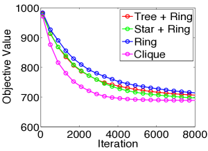
Figure 1: Objective value vs. number of iterations for different graph topologies. Note that larger the connectivity of the graph, faster is the convergence.

The results for Algorithm 1 on each topology for 10000 iterations are shown in Figure 1. The results clearly show that better connectivity implies better convergence rate. Note that while the clique topology has significantly better convergence than other topologies, acceptable long-term performance can be achieved by much sparser topologies such as Star + Ring and Tree + Ring.

Having a sparse communication graph is important to lower the cost of a distributed system. Furthermore, it is worth mentioning that the sparsity of the communication graph is also important in a multicore setting; since Algorithm 1 requires computing $(A_{i}A_{i}^{\top}+A_{j}A_{j}^{\top})^{+}$ for each communicating pair of nodes ($i$, $j$). Our analysis shows that this computation takes a significant portion of the running time and hence it is essential to minimize the number of variable pairs that are allowed to be updated.

6.2 Concurrency and Synchronization

As seen earlier, compared to Tree + Ring, Star + Ring is a low diameter layout (diameter = 2). Hence, in a sequential setting, it indeed results in a faster convergence. However, Star + Ring requires a node to be connected to all other nodes. This high-degree node could be a contention point in a parallel setting. We test the performance of our asynchronous algorithm in this setting. To assess how the performance would be affected with such contention and how asynchronous updates would increase performance, we conduct another experiment on the synthetic problem (12) but on a larger scale ($N=10000$, $x_{i}\in\mathbb{R}^{100}$, 100 constraints).

Our concurrent update follows a master/slave scheme. Each thread performs a loop where in each iteration it elects a master $i$ and slave $j$ and then applies the following sequence of actions:

1. Obtain the information required for the update from the master (i.e., information for calculating the gradients used for solving the subproblem).

2. Send the master information to the slave, update the slave variable and get back the information needed to update the master.

3. Update the master based (only) on the information obtained from steps 1 and 2.

We emphasize that the master is not allowed to read its own state at step 3 except to apply an increment, which is computed based on steps 1 and 2. This ensures that the master’s increment is consistent with that of the slave, even if one or both of them was being concurrently overwritten by another thread. More details on the implementation can be found in [12].

Given this update scheme, we experiment with three levels of synchronization: (a) Double Locking: Locks the master and the slave through the entire update. Because the objective function is decomposable, a more conservative locking (e.g. locking all nodes) is not needed. (b) Single Locking: Locks the master during steps 1 and 3 (the master is unlocked during step 2 and locks the slave during step 2). (c) Lock-free: No locks are used. Master and slave variables are updated through atomic increments similar to Hogwild! method.

Following [30], we use spinlocks instead of mutex locks to implement locking. Spinlocks are preferred over mutex locks when the resource is locked for a short period of time, which is the case in our algorithm. For each locking mechanism, we vary the number of threads from 1 to 15. We stop when $f_{0}-f_{t}>0.99(f_{0}-f^{*})$, where $f^{*}$ is computed beforehand up to three significant digits. Similar to [30], we add artificial delay to steps 1 and 2 in the update scheme to model complicated gradient calculations and/or network latency in a distributed setting.

Figure 2 shows the speedup for Tree + Ring and Star + Ring layouts. The figure clearly shows that a fully synchronous method suffers from contention in the Star + Ring topology whereas asynchronous method does not suffer from this problem and hence, achieves higher speedups. Although the Tree + Ring layouts achieves higher speedup than Star + Ring, the latter topology results in much less running time ($\sim$ 67 seconds vs 91 seconds using 15 threads).

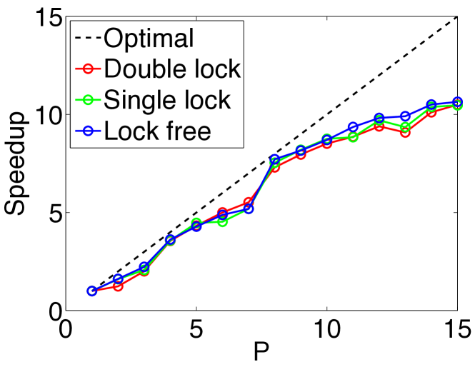
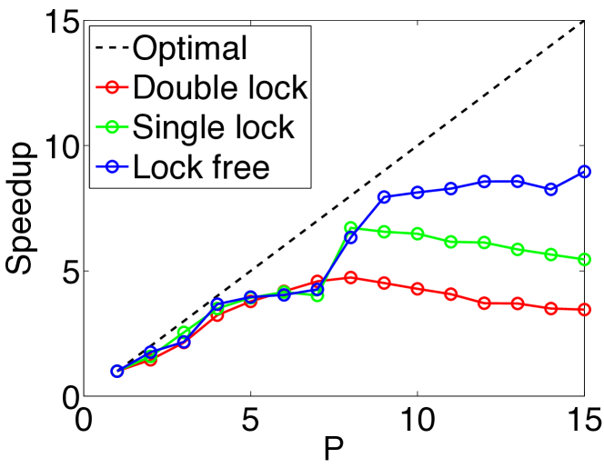
Figure 2: Speedup for Tree + Ring (top) and Star + Ring (bottom) topologies and different levels of synchronization. Note for Star + Ring topology, speedup of asynchronous algorithm is significantly higher than that of synchronous version.

6.3 Practical Case Study: Parallel Training of Linear SVM

In this section, we explore the effect of parallelism on randomized CD for training a linear SVM based on the dual formulation stated in (11). Necoara et. al. [22] have shown that, in terms of CPU time, a sequential randomized CD outperforms coordinate descent using Gauss-Southwell selection rule. It was also observed that randomized CD outperforms LIBSVM [6] for large datasets while maintaining reasonable performance for small datasets.

In this experiment we use a clique layout. For SVM training in a multicore setting, using a clique layout does not introduce additional cost compared to a more sparse layout. To maintain the box constraint, we use the double-locking scheme described in Section 6.2 for updating a pair of dual variables.

One advantage of coordinate descent algorithms is that they do not require the storage of the Gram matrix; instead they can compute its elements on the fly. That comes, however, at the expense of CPU time. Similar to [22], to speed up gradient computations without increasing memory requirements, we maintain the primal weight vector of the linear SVM and use it to compute gradients. Basically, if we increment $\alpha_{i}$ by $\delta_{i}$ and $\alpha_{j}$ by $\delta_{j}$, then we increment the weight vector by $\delta_{i}y_{i}x_{i}+\delta_{j}y_{j}x_{j}$. This increment is accomplished using atomic additions. However, this implies that all threads will be concurrently updating the primal weight vector. Similar to [30], we require these updates to be sparse with small overlap between non-zero coordinates in order to ensure convergence. In other words, we require training examples to have sparse features with small overlap between non-zero features.

We report speedups on two datasets used in [22]. Table 2 provides a description of both the datasets. For each dataset, we train the SVM model until $f_{0}-f_{t}>0.9999(f_{0}-f^{*})$, where $f^{*}$ is the objective reported in [22]. In Figure 3, we report speedup for both the datasets. The figure shows that parallelism indeed increases the performance of randomized CD training of linear SVM.

Dataset	# of instances	# of features	Avg # of non-zero features
a7a	16100	122	14
w8a	49749	300	12

Table 2: Datasets used for linear SVM Speedup experiment

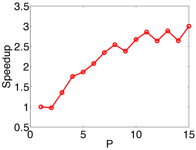
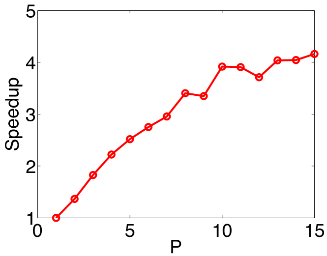
Figure 3: Speedup for linear SVM training on a7a (top) and w8a datasets.

7 DISCUSSION AND FUTURE WORK

We presented randomized coordinate descent methods for solving convex optimization problems with linear constraints that couple the variables. Moreover, we also presented composite objective, stochastic, and asynchronous versions of our basic method and provided their convergence analysis. We demonstrated the empirical performance of the algorithms. The experimental results of asynchronous algorithm look very promising.

There are interesting open problems for our problem in consideration: First, we would like to obtain high-probability results not just in expectation; another interesting direction is to extend the asynchronous algorithm to the non-smooth setting. Finally, while we obtain $O(1/k)$ for general convex functions, obtaining an accelerated $O(1/k^{2})$ rate is a natural question.

Acknowledgments

SS is partly supported by NSF grant: IIS-1409802. We thanks the anonymous reviewers for the helpful comments.

Appendix

Appendix A Proof of Theorem 3

Proof.

Taking the expectation over the choice of edges $(i_{k},j_{k})$ gives the following inequality

$$\mathbb{E}_{i_{k}j_{k}}[f(x^{k+1})|\eta_{k}] \leq\mathbb{E}_{i_{k}j_{k}}\left[f(x^{k})-\frac{1}{4L}\|\nabla_{y_{i_{k}}}f(x^{k})-\nabla_{y_{j_{k}}}f(x^{k})\|^{2}-\frac{1}{2L}\|\nabla_{z_{i_{k}}}f(x^{k})\|^{2}-\frac{1}{2L}\|\nabla_{z_{j_{k}}}f(x^{k})\|^{2}\right]$$

$$\leq f(x^{k})-\frac{1}{2}\nabla_{y}f(x^{k})^{\top}({\cal L}\otimes I_{n_{y}})\nabla_{y}f(x^{k})-\frac{1}{2}\nabla_{z}f(x^{k})^{\top}({\cal D}\otimes I_{n_{z}})\nabla_{z}f(x^{k})$$

$$\leq f(x^{k})-\frac{1}{2}\nabla f(x^{k})^{\top}\mathcal{K}\nabla f(x^{k}),$$ (13)

where $\otimes$ denotes the Kronecker product. This shows that the method is a descent method. Now we are ready to prove the main convergence theorem. We have the following:

$$f(x^{k+1})-f^{*} \leq\langle\nabla f(x^{k}),x^{k}-x^{*}\rangle\leq\|x^{k}-x^{*}\|_{\cal K}^{*}\|\nabla f(x^{k})\|_{\cal K}$$

$$\leq R(x^{0})\|\nabla f(x^{k})\|_{\cal K}\quad\forall k\geq 0.$$

Combining this with inequality (A), we obtain

$$\mathbb{E}[f(x^{k+1}|\eta_{k}]\leq f(x^{k})-\frac{(f(x^{k})-f^{*})^{2}}{2R^{2}(x^{0})}.$$

Taking the expectation of both sides an denoting $\Delta_{k}=\mathbb{E}[f(x^{k})]-f^{*}$ gives

$$\Delta_{k+1}\leq\Delta_{k}-\frac{\Delta_{k}^{2}}{2R^{2}(x^{0})}.$$

Dividing both sides by $\Delta_{k}\Delta_{k+1}$ and using the fact that $\Delta_{k+1}\leq\Delta_{k}$ we obtain

$$\frac{1}{\Delta_{k}}\leq\frac{1}{\Delta_{k+1}}-\frac{1}{2R^{2}(x^{0})}.$$

Adding these inequalities for $k$ steps $0\leq\frac{1}{\Delta_{0}}\leq\frac{1}{\Delta_{k}}-\frac{k}{2R^{2}(x^{0})}$ from which we obtain the statement of the theorem where $C=2R^{2}(x^{0})$. ∎

Appendix B Proof of Theorem 5

Proof.

In this case, the expectation should be over the selection of the pair $(i_{k},j_{k})$ and random index $l_{k}\in[N]$. In this proof, the definition of $\eta_{k}$ includes $l_{k}$ i.e., $\eta_{k}=\{(i_{0},j_{0},l_{0}),\dots,(i_{k-1},j_{k-1},l_{k-1})\}$. We define the following:

$$d_{i_{k}}^{k} =\left[\frac{\alpha_{k}}{2L}\left[\nabla_{y_{j_{k}}}f_{l_{k}}(x^{k})-\nabla_{y_{i_{k}}}f_{l_{k}}(x^{k})\right]^{\top},\quad-\frac{\alpha_{k}}{L}\left[\nabla_{z_{i_{k}}}f_{l_{k}}(x^{k})\right]^{\top}\right]^{\top},$$

$$d_{j_{k}}^{k} =\left[\frac{\alpha_{k}}{2L}\left[\nabla_{y_{j_{k}}}f_{l_{k}}(x^{k})-\nabla_{y_{i_{k}}}f_{l_{k}}(x^{k})\right]^{\top},\quad\frac{\alpha_{k}}{L}\left[\nabla_{z_{j_{k}}}f_{l_{k}}(x^{k})\right]^{\top}\right]^{\top},$$

$$d_{i_{k}j_{k}}^{l_{k}} =U_{i_{k}}d_{i_{k}}^{k}-U_{j_{k}}d_{j_{k}}^{k}.$$

For the expectation of objective value at $x^{k+1}$, we have

$$\mathbb{E}[f(x^{k+1})|\eta_{k}]\leq\mathbb{E}_{i_{k}j_{k}}\mathbb{E}_{l_{k}}\left[f(x^{k})+\left\langle\nabla f(x^{k}),d_{i_{k}j_{k}}^{l_{k}}\right\rangle+\frac{L}{2}\|d_{i_{k}j_{k}}^{l_{k}}\|^{2}\right]$$

$$\leq\mathbb{E}_{i_{k}j_{k}}\left[f(x^{k})+\left\langle\nabla f(x^{k}),\mathbb{E}_{l_{k}}[d_{i_{k}j_{k}}^{l_{k}}]\right\rangle+\frac{L}{2}\mathbb{E}_{l_{k}}[\|d_{i_{k}j_{k}}^{l_{k}}\|^{2}]\right]$$

$$\leq\mathbb{E}_{i_{k}j_{k}}\Big{[}f(x^{k})+\frac{\alpha_{k}}{2L}\left\langle\nabla_{y_{i_{k}}}f(x^{k}),\mathbb{E}_{l_{k}}[\nabla_{y_{j_{k}}}f_{l_{k}}(x^{k})-\nabla_{y_{i_{k}}}f_{l_{k}}(x^{k})]\right\rangle$$

$$\quad\quad+\frac{\alpha_{k}}{2L}\left\langle\nabla_{y_{j_{k}}}f(x^{k}),\mathbb{E}_{l_{k}}[\nabla_{y_{i_{k}}}f_{l_{k}}(x^{k})-\nabla_{y_{j_{k}}}f_{l_{k}}(x^{k})]\right\rangle$$

$$\quad\quad-\frac{\alpha_{k}}{L}\left\langle\nabla_{z_{i_{k}}}f(x^{k}),\mathbb{E}_{l_{k}}[\nabla_{z_{i_{k}}}f_{l_{k}}(x^{k})]\right\rangle-\frac{\alpha_{k}}{L}\left\langle\nabla_{z_{j_{k}}}f(x^{k}),\mathbb{E}_{l_{k}}[\nabla_{z_{j_{k}}}f_{l_{k}}(x^{k})]\right\rangle+\frac{L}{2}\mathbb{E}_{l_{k}}[\|d_{i_{k}j_{k}}^{l_{k}}\|^{2}]\Big{]}.$$

Taking expectation over $l_{k}$, we get the following relationship:

$$\mathbb{E}[f(x^{k+1})|\eta_{k}] \leq\mathbb{E}_{i_{k}j_{k}}\Big{[}f(x^{k})+\frac{\alpha_{k}}{2L}\left\langle\nabla_{y_{i_{k}}}f(x^{k}),\nabla_{y_{j_{k}}}f(x^{k})-\nabla_{y_{i_{k}}}f(x^{k})\right\rangle$$

$$\quad\quad+\frac{\alpha_{k}}{2L}\left\langle\nabla_{y_{j_{k}}}f(x^{k}),\nabla_{y_{i_{k}}}f(x^{k})-\nabla_{y_{j_{k}}}f(x^{k})\right\rangle$$

$$\quad\quad-\frac{\alpha_{k}}{L}\left\langle\nabla_{z_{i_{k}}}f(x^{k}),\nabla_{z_{i_{k}}}f(x^{k})\right\rangle-\frac{\alpha_{k}}{L}\left\langle\nabla_{z_{j_{k}}}f(x^{k}),\nabla_{z_{j_{k}}}f(x^{k})\right\rangle+\frac{L}{2}\mathbb{E}_{l_{k}}[\|d_{i_{k}j_{k}}^{l_{k}}\|^{2}]\Big{]}.$$

We first note that $\mathbb{E}_{l_{k}}[\|d_{i_{k}j_{k}}^{l_{k}}\|^{2}]\leq 8M^{2}\alpha_{k}^{2}/L^{2}$ since $\|\nabla f_{l}\|\leq M$. Substituting this in the above inequality and simplifying we get,

$$\mathbb{E}[f(x_{k+1})|\eta_{k}] \leq f(x^{k})-\alpha_{k}\nabla_{y}f(x^{k})^{\top}({\cal L}\otimes I_{n})\nabla_{y}f(x^{k})-\alpha_{k}\nabla_{z}f(x^{k})^{\top}({\cal D}\otimes I_{n})\nabla_{z}f(x^{k})+\frac{4M^{2}\alpha_{k}^{2}}{L}$$

$$\leq f(x^{k})-\alpha_{k}\nabla f(x^{k})^{\top}\mathcal{K}\nabla f(x^{k})+\frac{4M^{2}\alpha_{k}^{2}}{L}.$$ (14)

Similar to Theorem 3, we obtain a lower bound on $\nabla f(x^{k})^{\top}\mathcal{K}\nabla f(x^{k})$ in the following manner.

$$f(x^{k})-f^{*} \leq\langle\nabla f(x^{k}),x^{k}-x^{*}\rangle\leq\|x^{k}-x^{*}\|_{\cal K}^{*}.\|\nabla f(x^{k})\|_{\cal K}$$

$$\leq R(x^{0})\|\nabla f(x^{k})\|_{\cal K}.$$

Combining this with inequality Equation B, we obtain

$$\mathbb{E}[f(x_{k+1})|\eta_{k}]\leq f(x^{k})-\alpha_{k}\frac{(f(x^{k})-f^{*})^{2}}{R^{2}(x^{0})}+\frac{4M^{2}\alpha_{k}^{2}}{L}.$$

Taking the expectation of both sides an denoting $\Delta_{k}=\mathbb{E}[f(x^{k})]-f^{*}$ gives

$$\Delta_{k+1}\leq\Delta_{k}-\alpha_{k}\frac{\Delta_{k}^{2}}{R^{2}(x^{0})}+\frac{4M^{2}\alpha_{k}^{2}}{L}.$$

Adding these inequalities from $i=0$ to $i=k$ and use telescopy we get,

$$\Delta_{k+1}+\sum_{i=0}^{k}\alpha_{i}\frac{\Delta_{k}^{2}}{R^{2}(x^{0})}\leq\Delta_{0}+\frac{4M^{2}}{L}\sum_{i=0}^{k}\alpha_{i}^{2}.$$

Using the definition of $\bar{x}_{k+1}=\arg\min_{0\leq i\leq k+1}f(x_{i})$, we get

$$\sum_{i=0}^{k}\alpha_{i}\frac{(\mathbb{E}[f(\bar{x}_{k+1})-f^{*}])^{2}}{R^{2}(x^{0})}\leq\Delta_{k+1}+\sum_{i=0}^{k}\alpha_{i}\frac{\Delta_{k}^{2}}{R^{2}(x^{0})}\leq\Delta_{0}+\frac{4M^{2}}{L}\sum_{i=0}^{k}\alpha_{i}^{2}.$$

Therefore, from the above inequality we have,

$$\mathbb{E}[f(\bar{x}_{k+1})-f^{*}]\leq R(x^{0})\sqrt{\frac{(\Delta_{0}+4M^{2}\sum_{i=0}^{k}\alpha_{i}^{2}/L)}{\sum_{i=0}^{k}\alpha_{i}}}.$$

Note that $\mathbb{E}[f(\bar{x}_{k+1})-f^{*}]\rightarrow 0$ if we choose step sizes satisfying the condition that $\sum_{i=0}^{\infty}\alpha_{i}=\infty$ and $\sum_{i=0}^{\infty}\alpha_{i}^{2}<\infty$. Substituting $\alpha_{i}=\sqrt{\Delta_{0}L}/(2M\sqrt{i+1})$, we get the required result using the reasoning from [24] (we refer the reader to Section 2.2 of [24] for more details). ∎

Appendix C Proof of Theorem 4

Proof.

For ease of exposition, we analyze the case where the unconstrained variables $z$ are absent. The analysis of case with $z$ variables can be carried out in a similar manner. Consider the update on edge $(i_{k},j_{k})$. Recall that $D(k)$ denotes the index of the iterate used in the $k^{\text{th}}$ iteration for calculating the gradients. Let $d^{k}=\frac{\alpha_{k}}{2L}\left(\nabla_{y_{j_{k}}}f(x^{D(k)})-\nabla_{y_{i_{k}}}f(x^{D(k)})\right)$ and $d_{i_{k}j_{k}}^{k}=x^{k+1}-x^{k}=U_{i_{k}}d^{k}-U_{j_{k}}d^{k}$. Note that $\|d_{i_{k}j_{k}}^{k}\|^{2}=2\|d^{k}\|^{2}$. Since $f$ is Lipschitz continuous gradient, we have

$$f(x^{k+1}) \leq f(x^{k})+\left\langle\nabla_{y_{i_{k}}y_{j_{k}}}f(x^{k}),d_{i_{k}j_{k}}^{k}\right\rangle+\frac{L}{2}\|d_{i_{k}j_{k}}^{k}\|^{2}$$

$$\leq f(x^{k})+\left\langle\nabla_{y_{i_{k}}y_{j_{k}}}f(x^{D(k)})+\nabla_{y_{i_{k}}y_{j_{k}}}f(x^{k})-\nabla_{y_{i_{k}}y_{j_{k}}}f(x^{D(k)}),d_{i_{k}j_{k}}^{k}\right\rangle+\frac{L}{2}\|d_{i_{k}j_{k}}^{k}\|^{2}$$

$$\leq f(x^{k})-\frac{L}{\alpha_{k}}\|d_{i_{k}j_{k}}^{k}\|^{2}+\left\langle\nabla_{y_{i_{k}}y_{j_{k}}}f(x^{k})-\nabla_{y_{i_{k}}y_{j_{k}}}f(x^{D(k)}),d_{i_{k}j_{k}}^{k}\right\rangle+\frac{L}{2}\|d_{i_{k}j_{k}}^{k}\|^{2}$$

$$\leq f(x^{k})-L\left(\frac{1}{\alpha_{k}}-\frac{1}{2}\right)\|d_{i_{k}j_{k}}^{k}\|^{2}+\|\nabla_{y_{i_{k}}y_{j_{k}}}f(x^{k})-\nabla_{y_{i_{k}}y_{j_{k}}}f(x^{D(k)})\|\|d_{i_{k}j_{k}}^{k}\|$$

$$\leq f(x^{k})-L\left(\frac{1}{\alpha_{k}}-\frac{1}{2}\right)\|d_{i_{k}j_{k}}^{k}\|^{2}+L\|x^{k}-x^{D(k)}\|\|d_{i_{k}j_{k}}^{k}\|.$$

The third and fourth steps in the above derivation follow from definition of $d_{ij}^{k}$ and Cauchy-Schwarz inequality respectively. The last step follows from the fact the gradients are Lipschitz continuous. Using the assumption that staleness in the variables is bounded by $\tau$, i.e., $k-D(k)\leq\tau$ and definition of $d_{ij}^{k}$, we have

$$f(x^{k+1}) \leq f(x^{k})-L\left(\frac{1}{\alpha_{k}}-\frac{1}{2}\right)\|d_{i_{k}j_{k}}^{k}\|^{2}+L\left(\sum_{t=1}^{\tau}\|d_{i_{k-t}j_{k-t}}^{k-t}\|\|d_{i_{k}j_{k}}^{k}\|\right)$$

$$\leq f(x^{k})-L\left(\frac{1}{\alpha_{k}}-\frac{1}{2}\right)\|d_{i_{k}j_{k}}^{k}\|^{2}+\frac{L}{2}\left(\sum_{t=1}^{\tau}\left[\|d_{i_{k-t}j_{k-t}}^{k-t}\|^{2}+\|d_{i_{k}j_{k}}^{k}\|^{2}\right]\right)$$

$$\leq f(x^{k})-L\left(\frac{1}{\alpha_{k}}-\frac{1+\tau}{2}\right)\|d_{i_{k}j_{k}}^{k}\|^{2}+\frac{L}{2}\sum_{t=1}^{\tau}\|d_{i_{k-t}j_{k-t}}^{k-t}\|^{2}.$$

The first step follows from triangle inequality. The second inequality follows from fact that $ab\leq(a^{2}+b^{2})/2$. Using expectation over the edges, we have

$$\mathbb{E}[f( x^{k+1})]\leq\mathbb{E}[f(x^{k})]-L\left(\frac{1}{\alpha_{k}}-\frac{1+\tau}{2}\right)\mathbb{E}[\|d_{i_{k}j_{k}}^{k}\|^{2}]+\frac{L}{2}\mathbb{E}\left[\sum_{t=1}^{\tau}\|d_{i_{k-t}j_{k-t}}^{k-t}\|^{2}\right].$$ (15)

We now prove that, for all $k\geq 0$

$$\mathbb{E}\left[\|d_{i_{k-1}j_{k-1}}^{k-1}\|^{2}\right]\leq\rho\mathbb{E}\left[\|d_{i_{k}j_{k}}^{k}\|^{2}\right],$$ (16)

where we define $\mathbb{E}\left[\|d_{i_{k-1}j_{k-1}}^{k-1}\|^{2}\right]=0$ for $k=0$. Let $w^{t}$ denote the vector of size $|E|$ such that $w_{ij}^{t}=\sqrt{p_{ij}}\|d_{ij}^{t}\|$ (with slight abuse of notation, we use $w^{t}_{ij}$ to denote the entry corresponding to edge $(i,j)$). Note that $\mathbb{E}\left[\|d_{i_{t}j_{t}}^{t}\|^{2}\right]=\mathbb{E}[\|w^{t}\|^{2}]$. We prove Equation (16) by induction.

Let $u^{k}$ be a vector of size $|E|$ such that $u_{ij}^{k}=\sqrt{p_{ij}}\|d_{ij}^{k}-d_{ij}^{k-1}\|$. Consider the following:

$$\mathbb{E}[\|w^{k-1}\|]^{2}-\mathbb{E}[\|w^{k}\|^{2}] =\mathbb{E}[2\|w^{k-1}\|]^{2}-\mathbb{E}[\|w^{k}\|^{2}+\|w^{k-1}\|^{2}]$$

$$\leq 2\mathbb{E}[\|w^{k-1}\|^{2}]-2\mathbb{E}[\langle w^{k-1},w^{k}\rangle]$$

$$\leq 2\mathbb{E}[\|w^{k-1}\|\|w^{k-1}-w^{k}\|]$$

$$\leq 2\mathbb{E}[\|w^{k-1}\|\|u^{k}\|]\leq 2\mathbb{E}[\|w^{k-1}\|\sqrt{2}\alpha_{k}\|x^{D(k)}-x^{D(k-1)}\|]$$

$$\leq\sqrt{2}\alpha_{k}\sum_{t=\min(D(k-1),D(k))}^{\max(D(k-1),D(k))}\left(\mathbb{E}[\|w^{k-1}\|^{2}]+\mathbb{E}[\|d_{i_{t}j_{t}}^{t}\|^{2}]\right).$$ (17)

The fourth step follows from the bound below on $|u^{k}_{ij}|$

$$|u^{k}_{ij}| =\sqrt{p_{ij}}\|d_{ij}^{k}-d_{ij}^{k-1}\|$$

$$\leq\sqrt{p_{ij}}\|(U_{i}-U_{j})\frac{\alpha_{k}}{2L}(\nabla_{y_{i}}f(x^{D(k)})-\nabla_{y_{j}}f(x^{D(k)})+\nabla_{y_{j}}f(x^{D(k-1)})-\nabla_{y_{i}}f(x^{D(k-1)}))\|$$

$$\leq\sqrt{2p_{ij}}\alpha_{k}\|x^{D(k)}-x^{D(k-1)}\|.$$

The fifth step follows from triangle inequality. We now prove (16): the induction hypothesis is trivially true for $k=0$. Assume it is true for some $k-1\geq 0$. Now using Equation (C), we have

$$\mathbb{E}[\|w^{k-1}\|]^{2}-\mathbb{E}[\|w^{k}\|^{2}]\leq\sqrt{2}\alpha_{k}(\tau+2)\mathbb{E}[\|w^{k-1}\|^{2}]+\sqrt{2}\alpha_{k}(\tau+2)\rho^{\tau+1}\mathbb{E}[\|w^{k}\|^{2}]$$

for our choice of $\alpha_{k}$. The last step follows from the fact that $\mathbb{E}[\|d_{i_{t}j_{t}}^{t}\|^{2}]=\mathbb{E}[\|w^{t}\|^{2}]$ and mathematical induction. From the above, we get

$$\mathbb{E}[\|w^{k-1}\|^{2}]\leq\frac{1+\sqrt{2}{\alpha_{k}}(\tau+2)\rho^{(\tau+1)}}{1-\sqrt{2}{\alpha_{k}}(\tau+2)}\mathbb{E}[\|w^{k}\|^{2}]\leq\rho\mathbb{E}[\|w^{k}\|^{2}].$$

Thus, the statement holds for $k$. Therefore, the statement holds for all $k\in\mathbb{N}$ by mathematical induction. Substituting the above in Equation (15), we get

$$\mathbb{E}[f( x^{k+1})]\leq\mathbb{E}[f(x^{k})]-L\left(\frac{1}{\alpha_{k}}-\frac{1+\tau+\tau\rho^{\tau}}{2}\right)\mathbb{E}[\|d_{i_{k}j_{k}}^{k}\|^{2}].$$

This proves that the method is a descent method in expectation. Using the definition of $d_{ij}^{k}$, we have

$$\mathbb{E}[f(x^{k+1})] \leq\mathbb{E}[f(x^{k})]-\frac{\alpha_{k}^{2}}{4L}\left(\frac{1}{\alpha_{k}}-\frac{1+\tau+\tau\rho^{\tau}}{2}\right)\mathbb{E}[\|\nabla_{y_{i_{k}}}f(x^{D(k)})-\nabla_{y_{j_{k}}}f(x^{D(k)})\|^{2}]$$

$$\leq\mathbb{E}[f(x^{k})]-\frac{\alpha_{k}^{2}}{4L}\left(\frac{1}{\alpha_{k}}-\frac{1+\tau+\tau\rho^{\tau}}{2}\right)\mathbb{E}[\|\nabla f(x^{D(k)})-\nabla f(x^{D(k)})\|_{\cal K}^{2}]$$

$$\leq\mathbb{E}[f(x^{k})]-\frac{\alpha_{k}^{2}}{2R^{2}(x^{0})}\left(\frac{1}{\alpha_{k}}-\frac{1+\tau+\tau\rho^{\tau}}{2}\right)\mathbb{E}[(f(x^{D(k)})-f^{*})^{2}]$$

$$\leq\mathbb{E}[f(x^{k})]-\frac{\alpha_{k}^{2}}{2R^{2}(x^{0})}\left(\frac{1}{\alpha_{k}}-\frac{1+\tau+\tau\rho^{\tau}}{2}\right)\mathbb{E}[(f(x^{k})-f^{*})^{2}].$$

The second and third steps are similar to the proof of Theorem 3. The last step follows from the fact that the method is a descent method in expectation. Following similar analysis as Theorem 3, we get the required result. ∎

Appendix D Proof of Theorem 6

Proof.

Let $Ax=\sum_{i}x_{i}$. Let $\tilde{x}_{k+1}$ be solution to the following optimization problem:

$$\tilde{x}^{k+1}=\arg\min_{\{x|Ax=0\}}\langle\nabla f(x^{k}),x-x^{k}\rangle+\frac{L}{2}\|x-x^{k}\|^{2}+h(x).$$

To prove our result, we first prove few intermediate results. We say vectors $d\in\mathbb{R}^{n}$ and $d^{\prime}\in\mathbb{R}^{n}$ are conformal if $d_{i}d_{i}^{\prime}\geq 0$ for all $i\in[b]$. We use $d_{i_{k}j_{k}}=x^{k+1}-x^{k}$ and $d=\tilde{x}^{k+1}-x^{k}$. Our first claim is that for any $d$, we can always find conformal vectors whose sum is $d$ (see [22]). More formally, we have the following result.

Lemma 7.

For any $d\in\mathbb{R}^{n}$ with $Ad=0$, we have a multi-set $S=\{d_{ij}^{\prime}\}_{i\neq j}$ such that $d$ and $d_{ij}^{\prime}$ are conformal for all $i\neq j$ and $i,j\in[b]$ i.e., $\sum_{i\neq j}d_{ij}^{\prime}=d$, $Ad_{ij}^{\prime}=0$ and $d_{ij}^{\prime}$ can be non-zero only in coordinates corresponding to $x_{i}$ and $x_{j}$.

Proof.

We prove by an iterative construction, i.e., for every vector $d$ such that $Ad=0$, we construct a set $S=\{s_{ij}\}$ ($s_{ij}\in\mathbb{R}^{n}$) with the required properties. We start with a vector $u^{0}=d$ and multi-set $S^{0}=\{s^{0}_{ij}\}$ and $s^{0}_{ij}=0$ for all $i\neq j$ and $i,j\in[n]$. At the $k^{\text{th}}$ step of the construction, we will have $Au^{k}=0$, $As=0$ for all $s\in S^{k}$, $d=u^{k}+\sum_{s\in S^{k}}s$ and each element of $s$ is conformal to $d$.

In $k^{\text{th}}$ iteration, pick the element with the smallest absolute value (say $v$) in $u^{k-1}$. Let us assume it corresponds to $y_{p}^{j}$. Now pick an element from $u^{k-1}$ corresponding to $y_{q}^{j}$ for $p\neq q\in[m]$ with at least absolute value $v$ albeit with opposite sign. Note that such an element should exist since $Au^{k-1}=0$. Let $p_{1}$ and $p_{2}$ denote the indices of these elements in $u^{k-1}$. Let $S^{k}$ be same as $S^{k-1}$ except for $s^{k}_{pq}$ which is given by $s^{k}_{pq}=s^{k-1}_{pq}+r=s^{k-1}_{pq}+u_{p_{1}}^{k-1}e_{p_{1}}-u_{p_{1}}^{k-1}e_{p_{2}}$ where $e_{i}$ denotes a vector in $\mathbb{R}^{n}$ with zero in all components except in $i^{\text{th}}$ position (where it is one). Note that $Ar=0$ and $r$ is conformal to $d$ since it has the same sign. Let $u^{k+1}=u^{k}-r$. Note that $Au^{k+1}=0$ since $Au^{k}=0$ and $Ar=0$. Also observe that $As=0$ for all $s\in S^{k+1}$ and $u^{k+1}=\sum_{s\in S^{k}}s=d$.

Finally, note that each iteration the number of non-zero elements of $u^{k}$ decrease by at least 1. Therefore, this algorithm terminates after a finite number of iterations. Moreover, at termination $u^{k}=0$ otherwise the algorithm can always pick an element and continue with the process. This gives us the required conformal multi-set. ∎

Now consider a set $\{d_{ij}^{\prime}\}$ which is conformal to $d$. We define $\hat{x}_{k+1}$ in the following manner:

$$\hat{x}^{k+1}_{i}=\left\{\begin{array}[]{l l}x^{k}_{i}+d_{ij}^{\prime}&\quad\text{if $(i,j)=(i_{k},j_{k})$}\\ x^{k}_{i}&\quad\text{if $(i,j)\neq(i_{k},j_{k})$}\end{array}\right.$$

Lemma 8.

For any $x\in\mathbb{R}^{n}$ and $k\geq 0$,

$$\mathbb{E}[\|\hat{x}^{k+1}-x^{k}\|^{2}\leq\lambda(\|\tilde{x}^{k+1}-x^{k}\|^{2}).$$

We also have

$$\mathbb{E}(h(\hat{x}^{k+1}))\leq(1-\lambda)h(x^{k})+\lambda h(\tilde{x}^{k+1}).$$

Proof.

We have the following bound:

$$\mathbb{E}_{i_{k}j_{k}}[\|\hat{x}^{k+1}-x^{k}\|^{2} =\lambda\sum_{i\neq j}\|d_{ij}^{\prime}\|^{2}\leq\lambda\|\sum_{i\neq j}d_{ij}^{\prime}\|^{2}=\lambda\|d\|^{2}=\lambda\|\tilde{x}^{k+1}-x^{k}\|^{2}.$$

The above statement directly follows the fact that $\{d_{ij}^{\prime}\}$ is conformal to $d$. The remaining part directly follows from [22]. ∎

The remaining part essentially on similar lines as [22]. We give the details here for completeness. From Lemma 1, we have

$$\mathbb{E}_{i_{k}j_{k}}[F(x^{k+1})] \leq\mathbb{E}_{i_{k}j_{k}}[f(x^{k})+\langle\nabla f(x^{k}),d_{i_{k}j_{k}}\rangle+\frac{L}{2}\|d_{i_{k}j_{k}}\|^{2}+h(x^{k}+d_{i_{k}j_{k}})]$$

$$\leq\mathbb{E}_{i_{k}j_{k}}[f(x^{k})+\langle\nabla f(x^{k}),d_{i_{k}j_{k}}^{\prime}\rangle+\frac{L}{2}\|d_{i_{k}j_{k}}^{\prime}\|^{2}+h(x^{k}+d_{i_{k}j_{k}}^{\prime})]$$

$$=f(x^{k})+\lambda\left(\langle\nabla f(x),\sum_{i\neq j}d_{ij}^{\prime}\rangle+\sum_{i\neq j}\frac{L}{2}\|d_{ij}^{\prime}\|^{2}+\sum_{i\neq j}h(x+d_{ij}^{\prime})\right)$$

$$\leq(1-\lambda)F(x^{k})+\lambda(f(x^{k})+\langle\nabla f(x),d\rangle+\frac{L}{2}\|d\|^{2}+h(x+d))$$

$$\leq\min_{\{y|Ay=0\}}(1-\lambda)F(x^{k})+\lambda(F(y)+\frac{L}{2}\|y-x^{k}\|^{2})$$

$$\leq\min_{\beta\in[0,1]}(1-\lambda)F(x^{k})+\lambda(F(\beta x^{*}+(1-\beta)x^{k})+\frac{\beta^{2}L}{2}\|x^{k}-x^{*}\|^{2})$$

$$\leq(1-\lambda)F(x^{k})+\lambda\left(F(x^{k})-\frac{2(F(x^{k})-F(x^{*}))^{2}}{LR^{2}(x^{0})}\right).$$

The second step follows from optimality of $d_{i_{k}j_{k}}$. The fourth step follows from Lemma 8. Now using the similar recurrence relation as in Theorem 2, we get the required result. ∎

Appendix E Reduction of General Case

In this section we show how to reduce a problem with linear constraints to the form of Problem 4 in the paper. For simplicity, we focus on smooth objective functions. However, the formulation can be extended to composite objective functions along similar lines. Consider the optimization problem

$$\min_{x} \ f(x)$$

$$s.t.\ Ax= \sum A_{i}x_{i}=0,$$

where $f_{i}$ is a convex function with an $L$-Lipschitz gradient.

Let $\bar{A_{i}}$ be a matrix with orthonormal columns satisfying $\mathrm{range}(\bar{A_{i}})=\ker({A_{i}})$ , this can be obtained (e.g. using SVD). For each $i$, define $y_{i}=A_{i}x_{i}$ and assume that the rank of $A_{i}$ is less than or equal to the dimensionality of $x_{i}$. Then we can rewrite $x$ as a function $h(y,z)$ satisfying

$$x_{i}=A_{i}^{+}y_{i}+\bar{A_{i}}z_{i},$$

for some unknown $z_{i}$, where $C^{+}$ denote the pseudo-inverse of $C$. The problem then becomes

$$\min_{y,z}g(y,z)\ \ s.t.\ \sum_{i=1}^{N}y_{i}=0,$$ (18)

where

$$g(y,z)=f(\phi(y,z))=f\left(\sum_{i}U_{i}(A_{i}^{+}y_{i}+\bar{A_{i}}z_{i})\right).$$ (19)

It is clear that the sets $S_{1}=\{x|Ax=0\}$ and $S_{2}=\{\phi(y,z)|\sum_{i}y_{i}=0\}$ are equal and hence the problem defined in 18 is equivalent to that in 1.

Note that such a transformation preserves convexity of the objective function. It is also easy to show that it preserves the block-wise Lipschitz continuity of the gradients as we prove in the following result.

Lemma 9.

Let $f$ be a function with $L_{i}$-Lipschitz gradient w.r.t $x_{i}$. Let $g(y,z)$ be the function defined in 19. Then $g$ satisfies the following condition

$$\|\nabla_{y_{i}}g(y,z)-\nabla_{y_{i}}g(y^{\prime},z)\|\leq\frac{L_{i}}{\sigma_{\min}^{2}(A_{i})}\|y_{i}-y_{i}^{\prime}\|$$

$$\|\nabla_{z_{i}}g(y,z)-\nabla_{z_{i}}g(y,z^{\prime})\|\leq L_{i}\|z_{i}-z_{i}^{\prime}\|,$$

where $\sigma_{\min}(B)$ denotes the minimum non-zero singular value of $B$.

Proof.

We have

$$\|\nabla_{y_{i}}g(y,z)-\nabla_{y_{i}}g(y^{\prime},z)\| =\|(U_{i}A_{i}^{+})^{\top}[\nabla_{x}f(\phi(y,z))-\nabla_{x}f(\phi(y^{\prime},z))]\|$$

$$\leq\|A_{i}^{+}\|\|\nabla_{i}f(\phi(y,z))-\nabla_{i}f(\phi(y^{\prime},z))\|$$

$$\leq L_{i}\|A_{i}^{+}\|\|A_{i}^{+}(y_{i}-y_{i}^{\prime})\|\leq L_{i}\|A_{i}^{+}\|^{2}\|y_{i}-y_{i}^{\prime}\|=\frac{L_{i}}{\sigma_{\min}^{2}(A_{i})}\|y_{i}-y_{i}^{\prime}\|,$$

Similar proof holds for $\|\nabla_{z_{i}}g(y,z)-\nabla_{z_{i}}g(y,z^{\prime})\|$ , noting that $\|\bar{A_{i}}\|=1$. ∎

It is worth noting that this reduction is mainly used to simplify analysis. In practice, however, we observed that an algorithm that operates directly on the original variables $x_{i}$ (i.e. Algorithm 1) converges much faster and is much less sensitive to the conditioning of $A_{i}$ compared to an algorithm that operates on $y_{i}$ and $z_{i}$. Indeed, with appropriate step sizes, Algorithm 1 minimizes, in each step, a tighter bound on the objective function compared to the bound based 18 as stated in the following result.

Lemma 10.

Let $g$ and $\phi$ be as defined in 19. And let

$$d_{i}=A_{i}^{+}d_{y_{i}}+\bar{A_{i}}d_{z_{i}}.$$

Then, for any $d_{i}$ and $d_{j}$ satisfying $A_{i}d_{i}+A_{j}d_{j}=0$ and any feasible $x=\phi(y,z)$ we have

$$\langle\nabla_{i}f(x),d_{i}\rangle+\langle\nabla_{j}f(x),d_{j}\rangle+\frac{L_{i}}{2\alpha}\|d_{i}\|^{2}+\frac{L_{j}}{2\alpha}\|d_{j}\|^{2}$$

$$\leq\langle\nabla_{y_{i}}g(y,z),d_{y_{i}}\rangle+\langle\nabla_{z_{i}}g(y,z),d_{z_{i}}\rangle+\langle\nabla_{y_{j}}g(y,z),d_{y_{j}}\rangle+\langle\nabla_{z_{j}}g(y,z),d_{z_{j}}\rangle$$

$$+\frac{L_{i}}{2\alpha\sigma^{2}_{\min}(A_{i})}\|d_{y_{i}}\|^{2}+\frac{L_{i}}{2\alpha}\|d_{z_{i}}\|^{2}+\frac{L_{j}}{2\alpha\sigma^{2}_{\min}(A_{j})}\|d_{y_{j}}\|^{2}+\frac{L_{j}}{2\alpha}\|d_{z_{j}}\|^{2}.$$

Proof.

The proof follows directly from the fact that

$$\nabla_{i}f(x)={A_{i}^{+}}^{\top}\nabla_{y_{i}}g(y,z)+{\bar{A_{i}}}^{\top}\nabla_{z_{i}}g(y,z).$$

∎

References

- Auslender [1976] A. Auslender. Optimisation Méthodes Numériques. Masson, 1976.
- Beck and Tetruashvili [2013] A. Beck and L. Tetruashvili. On the convergence of block coordinate descent type methods. SIAM Journal on Optimization, 23(4):2037–2060, 2013. doi: 10.1137/120887679.
- Berman et al. [1992] P. Berman, N. Kovoor, and P. M. Pardalos. A linear-time algorithm for the least-distance problem. Technical report, Pennsylvania State University, Department of Computer Science, 1992.
- Bertsekas [1999] D. P. Bertsekas. Nonlinear Programming. Athena Scientific, Belmont, MA, second edition, 1999.
- Bradley et al. [2011] J. Bradley, A. Kyrola, D. Bickson, and C. Guestrin. Parallel coordinate descent for L1-regularized loss minimization. In L. Getoor and T. Scheffer, editors, Proceedings of the 28th International Conference on Machine Learning, pages 321–328. Omnipress, 2011.
- Chang and Lin [2011] C.-C. Chang and C.-J. Lin. Libsvm: A library for support vector machines. ACM Trans. Intell. Syst. Technol., 2(3):27:1–27:27, May 2011. ISSN 2157-6904. doi: 10.1145/1961189.1961199. URL http://doi.acm.org/10.1145/1961189.1961199.
- Fercoq and Richtárik [2013] O. Fercoq and P. Richtárik. Accelerated, parallel and proximal coordinate descent. CoRR, abs/1312.5799, 2013.
- Friedman et al. [2007] J. Friedman, T. Hastie, H. Höfling, R. Tibshirani, et al. Pathwise coordinate optimization. The Annals of Applied Statistics, 1(2):302–332, 2007.
- Gabay and Mercier [1976] D. Gabay and B. Mercier. A dual algorithm for the solution of nonlinear variational problems via finite element approximation. Computers & Mathematics with Applications, 2(1):17–40, 1976. doi: http://dx.doi.org/10.1016/0898-1221(76)90003-1. URL http://www.sciencedirect.com/science/article/pii/0898122176900031.
- Glowinski and Marrocco [1975] R. Glowinski and A. Marrocco. Sur l’approximation, par éléments finis d’ordre un, et la résolution, par pénalisation-dualité d’une classe de problèmes de dirichlet non linéares. Revue Française d’Automatique, Informatique, et Recherche Opérationelle, 1975.
- Golub and Van Loan [1996] G. H. Golub and C. F. Van Loan. Matrix Computations. John Hopkins University Press, Baltimore, MD, 3rd edition, 1996.
- Hefny et al. [2014] A. Hefny, S. Reddi, and S. Sra. Coordinate descent algorithms with coupling constraints: Lessons learned. In NIPS Workshop on Software Engineering For Machine Learning, 2014.
- Hong and Luo [2012] M. Hong and Z.-Q. Luo. On the linear convergence of the alternating direction method of multipliers. arXiv preprint arXiv:1208.3922, 2012.
- Hong et al. [2013] M. Hong, X. Wang, M. Razaviyayn, and Z.-Q. Luo. Iteration Complexity Analysis of Block Coordinate Descent Methods. arXiv:1310.6957, 2013.
- Hsieh and Dhillon [2011] C. J. Hsieh and I. S. Dhillon. Fast coordinate descent methods with variable selection for non-negative matrix factorization. In Proceedings of the 17th ACM SIGKDD International Conference on Knowledge Discovery and Data Mining(KDD), pages 1064–1072, August 2011.
- Hsieh et al. [2008] C. J. Hsieh, K. W. Chang, C. J. Lin, S. S. Keerthi, and S. Sundararajan. A dual coordinate descent method for large-scale linear SVM. In W. Cohen, A. McCallum, and S. Roweis, editors, ICML, pages 408–415. ACM, 2008.
- Hsieh et al. [2011] C.-J. Hsieh, M. A. Sustik, I. S. Dhillon, and P. D. Ravikumar. Sparse inverse covariance matrix estimation using quadratic approximation. In NIPS, pages 2330–2338, 2011.
- Lacoste-Julien et al. [2012] S. Lacoste-Julien, M. Jaggi, M. Schmidt, and P. Pletscher. Block-coordinate frank-wolfe optimization for structural svms. arXiv preprint arXiv:1207.4747, 2012.
- Lawson and Hanson [1974] C. L. Lawson and R. J. Hanson. Solving Least Squares Problems. Prentice–Hall, Englewood Cliffs, NJ, 1974. Reissued with a survey on recent developments by SIAM, Philadelphia, 1995.
- Liu et al. [2013] J. Liu, S. J. Wright, C. Ré, V. Bittorf, and S. Sridhar. An asynchronous parallel stochastic coordinate descent algorithm. arXiv:1311.1873, 2013.
- Luo and Tseng [1992] Z.-Q. Luo and P. Tseng. On the convergence of the coordinate descent method for convex differentiable minimization. Journal of Optimization Theory and Applications, 72(1):7–35, 1992.
- Necoara and Patrascu [2014] I. Necoara and A. Patrascu. A random coordinate descent algorithm for optimization problems with composite objective function and linear coupled constraints. Comp. Opt. and Appl., 57(2):307–337, 2014.
- Necoara et al. [2011] I. Necoara, Y. Nesterov, and F. Glineur. A random coordinate descent method on large optimization problems with linear constraints. Technical report, Technical Report, University Politehnica Bucharest, 2011, 2011.
- Nemirovski et al. [2009] A. Nemirovski, A. Juditsky, G. Lan, and A. Shapiro. Robust stochastic approximation approach to stochastic programming. SIAM J. on Optimization, 19(4):1574–1609, Jan. 2009. ISSN 1052-6234. doi: 10.1137/070704277.
- Nesterov [2010] Y. Nesterov. Efficiency of coordinate descent methods on huge-scale optimization problems. Core discussion papers, Université catholique de Louvain, Center for Operations Research and Econometrics (CORE), 2010.
- Nesterov [2012] Y. Nesterov. Efficiency of coordinate descent methods on huge-scale optimization problems. SIAM Journal on Optimization, 22(2):341–362, 2012.
- Platt [1998] J. C. Platt. Sequential minimal optimization: A fast algorithm for training support vector machines. Technical report, ADVANCES IN KERNEL METHODS - SUPPORT VECTOR LEARNING, 1998.
- Polyak [1987] B. T. Polyak. Introduction to Optimization. Optimization Software Inc., 1987. Nov 2010 revision.
- Rastrigin [1968] L. A. Rastrigin. Statisticheskie Metody Poiska Ekstremuma (Statistical Extremum Seeking Methods). Nauka, Moscow, 1968.
- Recht et al. [2011] B. Recht, C. Re, S. J. Wright, and F. Niu. Hogwild: A Lock-Free Approach to Parallelizing Stochastic Gradient Descent. In J. Shawe-Taylor, R. S. Zemel, P. L. Bartlett, F. C. N. Pereira, and K. Q. Weinberger, editors, NIPS, pages 693–701, 2011.
- Richtárik and Takáč [2013] P. Richtárik and M. Takáč. Distributed coordinate descent method for learning with big data. ArXiv e-prints, Oct. 2013.
- Richtárik and Takáč [2011] P. Richtárik and M. Takáč. Iteration complexity of randomized block-coordinate descent methods for minimizing a composite function. arXiv:1107.2848v1, July 2011.
- Richtárik and Takáč [2012] P. Richtárik and M. Takáč. Parallel coordinate descent methods for big data optimization. arXiv:1212.0873v1, Dec 2012.
- Saha and Tewari [2013] A. Saha and A. Tewari. On the nonasymptotic convergence of cyclic coordinate descent methods. SIAM Journal on Optimization, 23(1):576–601, 2013.
- Shalev-Shwartz and Zhang [2013a] S. Shalev-Shwartz and T. Zhang. Stochastic dual coordinate ascent methods for regularized loss minimization. JMLR, 14, 2013a.
- Shalev-Shwartz and Zhang [2013b] S. Shalev-Shwartz and T. Zhang. Accelerated mini-batch stochastic dual coordinate ascent. arXiv:1305.2581v1, 2013b.
- Tappenden et al. [2013] R. Tappenden, P. Richtárik, and J. Gondzio. Inexact coordinate descent: complexity and preconditioning. arXiv:1304.5530, 2013.
- Tibshirani et al. [2005] R. Tibshirani, M. Saunders, S. Rosset, J. Zhu, and K. Knight. Sparsity and smoothness via the fused lasso. Journal of the Royal Statistical Society: Series B (Statistical Methodology), 67(1):91–108, 2005.
- Tseng and Yun [2009] P. Tseng and S. Yun. A block-coordinate gradient descent method for linearly constrained nonsmooth separable optimization. Journal of Optimization Theory and Applications, 2009.
- Wang and Lin [2014] P.-W. Wang and C.-J. Lin. Iteration complexity of feasible descent methods for convex optimization. JMLR, 15:1523–1548, 2014.