Towards Knowledge-Enriched Path Computation

Abstract

Directions and paths, as commonly provided by navigation systems, are usually derived considering absolute metrics, e.g., finding the shortest path within an underlying road network. With the aid of crowdsourced geospatial data we aim at obtaining paths that do not only minimize distance but also lead through more popular areas using knowledge generated by users. We extract spatial relations such as “nearby” or “next to” from travel blogs, that define closeness between pairs of points of interest (PoIs) and quantify each of these relations using a probabilistic model. Subsequently, we create a relationship graph where each node corresponds to a PoI and each edge describes the spatial connection between the respective PoIs. Using Bayesian inference we obtain a probabilistic measure of spatial closeness according to the crowd. Applying this measure to the corresponding road network, we obtain an altered cost function which does not exclusively rely on distance, and enriches an actual road networks taking crowdsourced spatial relations into account. Finally, we propose two routing algorithms on the enriched road networks. To evaluate our approach, we use Flickr photo data as a ground truth for popularity. Our experimental results – based on real world datasets – show that the paths computed w.r.t. our alternative cost function yield competitive solutions in terms of path length while also providing more “popular” paths, making routing easier and more informative for the user.

1 Introduction

User-contributed content has benefited many scientific disciplines by providing a wealth of new data. Technological progress, especially smart phones and GPS receivers, has facilitated contributing to the plethora of available information. OpenStreetMap constitutes the standard example and reference in the area of volunteered geographic information. Authoring geospatial information typically implies coordinate-based, quantitative data. Contributing quantitative data requires specialized applications (often part of social media platforms) and/or specialized knowledge, as is the case with OpenStreetMap (OSM).

The broad mass of users contributing content, however, are much more comfortable using qualitative information. People typically do not use geographical coordinates to describe their spatial motion, for instance when traveling or roaming. Instead, they use qualitative information in the form of toponyms (landmarks) and spatial relationships (“near”, “next to”, “north of”, etc.). Hence, there is an abundance of geospatial information (freely) available on the Internet, e.g., in travel blogs, largely unused. In contrast to quantitative information, which is mathematically measurable (although sometimes flawed by measurement errors), qualitative information is based on personal cognition. Therefore, accumulated and processed qualitative information may better represent human way of thinking.

This is of particular interest when considering the “routing problem” (equivalent to “path finding”). Traditional routing queries use directions from systems that only take the structure of the underlying road network into account. In human interaction such information is usually enhanced with qualitative information (e.g. “the street next to the church”, “the bridge north of the Eiffel tower”). Combining traditional routing algorithms with crowdsourced – thus, more commonly used – geospatial references we aim to more properly represent human perception while keeping it mathematically measurable. In this work, we enrich a road network with information about spatial relations between pairs of Points of Interest (PoI) extracted from textual travel-blog data. Using these relations, we obtain routes that are easier to interpret and to follow, much rather resembling a route that a person would provide.

As an example, consider the routing scenario in Figure 1 which is set in the city of Paris, France. The continuous line represents the conventional shortest path from starting point “Gare du Nord” to the target at “Quai de la Rapée” –while the dot dashed and dotted lines represent alternative paths computed by the algorithms introduced in this paper. The triangles in this example denote touristic landmarks and sights. For instance, the dot dashed path on the bottom right passing recognizable locations such as “Place de la République”, “Cirque d’hiver” and “la Bastille”, as proposed by our algorithms, is considerably easier to describe and follow, and might yield more interesting sights for tourists than the shortest path.

The challenge of this work is to extract crowdsourced information from textual data and incorporate it an existing road network. This enriched road network is subsequently used to provide paths between a given start and target that satisfy the claim of higher popularity (which is formally introduced in Section 5), while only incurring a minor additional spatial distance. In addition to this main application, we note that our techniques can furthermore be used to automatically provide interesting tourist routes in any place where information about PoIs is publicly available.

The transition from textual information to routing in networks is not at all straightforward, therefore we employ and develop various methods from different angles of computing science:

• We begin by mining information from texts, employing Natural Language Processing methods in order to determine spatial entities and relations between them (cf. Section 3).

• Due to the inherent uncertainty of crowdsourced data, we employ probability distributions to quantitatively model spatial relations mined from the text (cf. Section 4).

• We propose a Bayesian inference-based transition from the probabilistically modeled spatial relations to confidence measurements about the quality of spatial relation extracted from text (cf. Section 5.1).

• We define a new cost criterion which is used to enrich an underlying road network with the aforementioned confidence measurements (cf. Section 5.2).

• Finally, we propose two algorithms which use the enriched road network to compute actual paths (cf. Section 5.3).

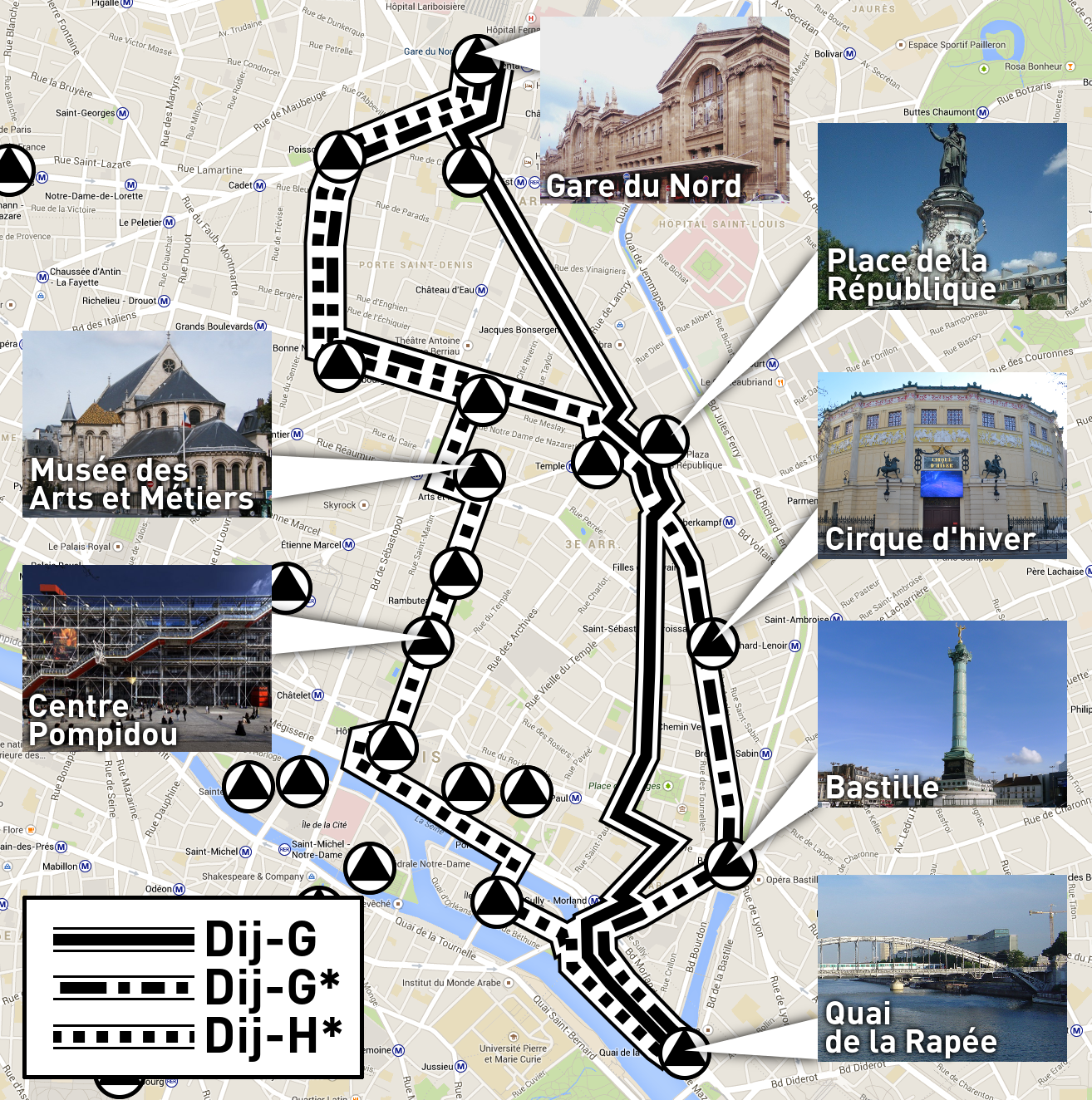
Figure 1: Shortest (continuous) and alternative paths (dot dashed and dotted) alongside PoIs in the city of Paris. This result is an output of the algorithms presented in this paper.

2 Related Work

Research areas relevant to this work include: $(i)$ qualitative routing and $(ii)$ mining of semantic information from moving object trajectories and trajectory enrichment with extracted semantic information. In what follows, we discuss previous work in both of these areas.

While finding shortest paths in road networks is a thoroughly explored research area, qualitative routing has hardly been explored. Nevertheless, providing meaningful routing directions in road networks is a research topic of great importance. In various real world scenarios, the shortest path may not be the ideal choice for providing directions in written or spoken form, for instance when in an unfamiliar neighborhood, or in cases of emergency. Rather, it is often more preferable to offer “simple” directions that are easy to memorize, explain, understand and follow. However, there exist cases where the simplest route is considerably longer than the shortest. The authors in [15], [4] and [19] try to tackle the problem of efficient routing by using cost functions that trade off between minimizing the length of a provided path while also minimizing the number of turns, e.g., number of instructions, of the provided path. The major shortcoming of these approaches is that they focus almost exclusively on road network data without taking into account any kind of qualitative information, i.e. information coming from the user. Opposed to that, we try to approach the problem of efficient routing by integrating spatial knowledge coming from the crowd thus enriching an actual road network.

The importance of landmark based routing from human cognition point of view, has been analyzed on a theoretical basis, e.g., without an real routing application, in [14] and [7]. The discovery of semantic places through the analysis of raw trajectory data has been investigated thoroughly over the course of the last years. The authors in [9], [20] and [11] provide solutions for the semantic place recognition problem and categorize the extracted PoIs into pre-defined types. Moreover, the concept of “semantic behavior” has recently been introduced. This refers to the use of semantic abstractions of the raw mobility data, including not only geometric patterns but also knowledge extracted jointly from the mobility data as well as the underlying geographic and application domains in order to understand the actual behavior of moving users. Several approaches like [1], [12], [17], [21], [17] and [22] have been introduced the last decade. The core contribution of these articles lies in the development of a semantic approach that progressively transforms the raw mobility data into semantic trajectories enriched with PoIs, segmentations and annotations. Moreover, a recent work, [5], can extract and transform the aforementioned semantic information into a text description in the form of a diary. Finally, the authors in [13] propose an approach for route recommendation based on a user opinion mining platform about trajectories, providing longer but more pleasant routes. The major drawback of these approaches is that they do not integrate the extracted semantic information into the road network. Instead, they use the extracted information only on specific trajectories. In our contribution, we analyze crowdsourced data in order to extract semantic spatial information and integrate it into an actual road network. This will enable us to provide routes that are near-optimal w.r.t. distance while spatially more popular according to the crowd.

3 Spatial Relation Extraction

In this work, we choose travel blogs as a rich potential source for (crowdsourced) geo-spatial data. This selection is based on the fact that people tend to describe their experiences in relation to their trips and places they have visited, which results in “spatial” narratives. To gather such data, we use classical Web crawling techniques and compile a database consisting of 120,000 texts, obtained from travel blogs.

Obtaining qualitative spatial relations from text involves the detection of $(i)$ PoIs (or toponyms) and $(ii)$ spatial relationships linking the PoIs. The employed approach involves geoparsing, i.e. the detection of candidate phrases, and geocoding, i.e., linking the phrases to actual coordinate information.

Using the Natural Language Processing Toolkit (NLTK) (cf. [8]), a leading platform for analyzing raw natural language data, we managed to extract 500,000 PoIs from the text corpus. For the geocoding of the PoIs, we rely on the GeoNames geographical gazetteer data, which contains over ten million PoI names worldwide and their coordinates. This procedure associates (whenever possible) PoIs found in the travel blogs with geo coordinates.Using the GeoNames gazetteer we were able to geocode about 480,000 out of the 500,000 extracted PoIs.

Having identified and geocoded the spatial objects, the next step is the extraction of qualitative spatial relationships. The extraction of spatial relations between entities in text is a hard Natural Language Processing (NLP) problem, especially when applied to a noisy crowdsourced dataset. We address this NLP challenge by implementing a spatial relation extraction algorithm based on NLTK [8] components in combination with predefined strings and syntactical patterns. More specifically, we define a set of language expressions that are typically used to express a spatial relation in combination with a set of syntactical rules. The use of both syntactical and string matching reduces the number of false positives considerably. As an example, consider the following phrase. “Deutsche Bank invested 10 million dollars in Brazil”. Here, a simple string matching solution would return a triplet of the form (Deutsche Bank, in, Brazil), which is a false positive. In our approach, the use of predefined syntactical patterns avoids this kind of mistakes.

Algorithm 1 describes the architecture of the proposed information extraction system. Initially, syntactical and string patterns are loaded (Step 2). The raw text document is segmented into sentences (Step 4). Each sentence is further subdivided (tokenized) into words and tagged as part-of-speech (Steps 6-7). Continuing, name entities (PoIs) are identified (Step 8). We look for relations between specified types of named entities, which in NLTK are Organizations, Locations, Facilities and Geo-Political Entities (GPEs). Next, in case there are two or more name entities in the sentence, we check if any of the predefined syntactical patterns applies between the recognized name entities pairs (Step 13). If it exists, we then use regular expressions to determine the specific spatial relation instance from our predefined spatial relation pattern list for this case. If there is a string pattern match we record the extracted triplet (Steps 15-16). Thus, the search for spatial relations in texts results into triplets of the form ($P_{i}$, $R^{k}$, $P_{j}$),

Input: A database of texts $\mathcal{T}$

Output: A set of triplets $\mathcal{O}=(P_{i},R^{k},P_{j})$ where $P_{i}\neq P_{j}$

1 begin

2       Load syntactical $\mathcal{A}$ and string $\mathcal{B}$ patterns

3      foreach text $t\in\mathcal{T}$ do

4             Extract sentences from $t$ into set $\mathcal{S}$

5            foreach sentence $s\in\mathcal{S}$ do

6                   Token $s$ using NLTK

7                   PosTag $s$ using NLTK

8                   Identify name entities using NLTK

9                  if two or more name entities in $s$ then

10                         Extract pairs in $\mathcal{P}$

11                        foreach $p\in\mathcal{P}$ do

12                               $p_{\mathcal{A}}\leftarrow$ Extract syntactical pattern of $p$

13                              if $p_{\mathcal{A}}\in\mathcal{A}$ then

14                                     $p_{\mathcal{B}}\leftarrow$ Extract string pattern of $p$

15                                    if $p_{\mathcal{B}}\in\mathcal{B}$ then

16                                           $\mathcal{O}.\proc{PushTriplet}(p(1),p_{\mathcal{B}},p(2))$

17                                     end if

18                                    

19                               end if

20                              

21                         end foreach

22                        

23                   end if

24                  

25             end foreach

26            

27       end foreach

28      

29      return $\mathcal{O}$

30      

31 end

Algorithm 1 Spatial Relation Extraction

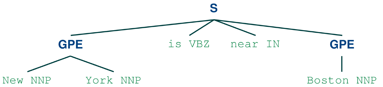
Figure 2: Example of a parsed sentence syntactic tree.

An example is shown in Figure 2, where a sentence is analyzed as explained and two named entities are identified as GPEs. We first check the syntax and make sure that the pattern “GPE - 3rd person verbal phrase (VBZ) - preposition/subordinating conjunction (IN) - GPE” exists in our set of predefined spatial relation patterns. Performing string matching on the intermediate chunks (“near”) results in the triplet (New York, Near, Boston). Applying Algorithm 1, we extracted 440,000 triplets from our 120,000 travel blog text corpus.

Figure 3 shows a Spatial Relationship Graph, i.e., a spatial graph in which nodes represent PoIs and edges label spatial relationships existing between them. The graph visualizes a small sample of spatial relationship data collected for the city of London. We have collected data for the regions of New York, Paris and London which will be our datasets during the experimental evaluation of the proposed approach. Here, we should point out that for the scope of this work, i.e. a combination of short and enriched routes, we only consider distance and topological relations that denote closeness (near, close, next to, at, in etc). The use of relations that denote direction, e.g. north, south, east etc., or remoteness, e.g. away from, far etc., is an open direction for future work.

Figure 3: Sample of a spatial relation graph for London.

4 Modeling Spatial Relations

In this section we describe the probabilistic modeling we follow in order to quantify the qualitative spatial relations between PoIs. Key ingredients of our system are methods that train probabilistic models, which is required due to the inherent uncertainty of crowdsourced data. Our discussion below includes a description of the features we used to model spatial relations and a short analysis of the modeling approach used in [16], i.e., the probabilistic mixture models we employ for the quantitative representation of spatial relations and a greedy learning algorithm for model parameter estimation. These spatial relations models are necessary to assess the quality of spatial relations extracted from text. The spatial relations and their corresponding quality information will be used in Section 5.2 for the enrichment of the underlying spatial network. This enrichment will be used to find paths which favor popular parts of the road network in Section 5.3.

4.1 Spatial Features

In this work, we model a spatial relation between two PoIs $P_{i}$ and $P_{j}$ in terms of distance and orientation as presented in [16]. Therefore, we extract occurrences of a spatial relation (such as “near”) from travel blogs as described in Section 3. For each occurrence, we create a two-dimensional spatial feature vector $D=(D_{d},D_{o})^{\intercal}$ where $D_{d}$ denotes the distance and $D_{o}$ denotes the orientation between $P_{i}$ and $P_{j}$. This way, we end up with a set of two-dimensional feature vectors $\mathcal{D}_{\text{rel}}=\{D_{1},D_{2},\dots,D_{n}\}$ for each spatial relation. An example of the feature extraction procedure is illustrated in Figure 4 (cf. [16]), where four instances of spatial relation near create the respective set of spatial feature vectors $\mathcal{D}_{\text{near}}=\{(D_{d1},D_{o1})^{\intercal},(D_{d2},D_{o2})^{\intercal},(D_{d3},D_{o3})^{\intercal},(D_{d4},D_{o4})^{\intercal}\}$.

Figure 4: Distance and orientation feature extraction procedure - B is near A, C is near D, F is near E and H is near G.

4.2 Probabilistic Models

Section 4.1 provides us, for each spatial relation such as “near” and “into”, with a set of distances and orientations of their instances. Using these instances, we employ Gaussian Mixture Models (GMMs) which have been extensively used in many classification and general machine learning problems ([2]). They are very well known for $(i)$ their formality, as they build on the formal probability theory, $(ii)$ their practicality, as they have been implemented several times in practice, $(iii)$ their generality, as they are capable of handling many different types of uncertainty, and $(iv)$ their effectiveness.

In general, a GMM is a weighted sum of $M$-component Gaussian densities as $p(d|\lambda)=\sum_{i=1}^{M}w_{i}g(d;\mu_{i},\Sigma_{i})$ where $d$ is a $l$-dimensional data vector (in our case $l=2$), $w_{i}$ are the mixture weights, and $g(d;\mu_{i},\Sigma_{i})$ is a Gaussian density function with mean vector $\mu_{i}\in\mathbb{R}^{l}$ and covariance matrix $\Sigma_{i}\in\mathbb{R}^{l\times l}$. To fully characterize the probability density function $p(d|\lambda)$, one requires the mean vectors, the covariance matrices and the mixture weights. These parameters are collectively represented in $\lambda=\{w_{i},\mu_{i},\Sigma_{i}\}$ for $i=1,\dots,M$.

In our setting, each spatial relation is modeled under a probabilistic framework by a 2-dimensional GMM, trained on each relation’s spatial feature vectors, as discussed in Section 4.1. For the parameter estimation of each Gaussian component of each GMM, we use Expectation Maximization (EM) ([3]). EM enables us to update the parameters of a given M-component mixture with respect to a feature vector set $\mathcal{D}_{\text{rel}}=\{D_{1},\dots,D_{n}\}$ with $1\leq j\leq n$ and all $D_{j}\in\mathbb{R}^{l}$, such that the log-likelihood given by Equation 1, increases with each re-estimation step, i.e., EM re-estimates model parameters $\lambda$ until convergence. A formal analysis of the parameter re-estimation formula for each EM step is given in the Appendix.

$$\mathcal{L}=\sum_{j=1}^{n}\log(p(D_{j}|\lambda))$$ (1)

A main issue in probabilistic modeling with probability mixtures is that a predefined number of components is neither a dynamic nor an efficient and robust approach. The optimal number of components should be decided based on each dataset. We employ a greedy learning approach to dynamically estimate the number of components in a GMM. This approach builds the mixture component in an efficient way by starting from an one-component GMM—whose parameters are trivially computed by using EM— and then employing the following two basic steps until a stopping criterion is met:

1. Insert a new component in the mixture

2. Apply EM until the log-likelihood $\mathcal{L}$ or the parameters of the GMM converge

The stopping criterion can either be a maximum pre-selected number of components, or it can be any other model selection criterion. In our case, the algorithm stops if the maximum number of components is reached, or if the new model’s log-likelihood $\mathcal{L}+1$ is less or equal to the log-likelihood $\mathcal{L}$ of the previous model, after introducing a new component. A detailed description of the optimized GMM training algorithm is given in [18].

5 ROAD NETWORK ENRICHMENT

In this section we describe our approach to enrich an actual road network with crowdsourced spatial information. Our discussion below includes a description of how we transform a relationship graph, as presented in Section 3, into a weighted graph, and how we use the edge weights of the weighted graph in order to modify the edge costs of a real road network.

5.1 From Relationship to Weighted Graphs

As presented in Section 3, the spatial relation extraction procedure results in a relationship graph between PoIs such as the relationship graph of Figure 3. A simpler example of such a graph is shown in Figure 5. In general, let $\mathcal{P}=\{P_{1},\dots,P_{m}\}$ denote the set of nodes representing the PoIs and let $\mathcal{R}=\{R^{1},\dots,R^{n}\}$ denote the pre-defined set of spatial closeness relations, represented by spatial NLP expressions like “next to” or “close by”. Furthermore, let $R_{i,j}\subseteq\mathcal{R}$ denote the set of relations observed (i.e. extracted from the text) between two distinct nodes $P_{i}$ and $P_{j}$. Note that $R^{k}$ denotes an abstract relation, while $R_{i,j}$ denotes a set of occurrences of relations between a pair of nodes. Let $D_{i,j}$ denote the spatial feature vector (distance and orientation), between two distinct PoIs $P_{i}$ and $P_{j}$ (as presented in Section 4.1). Finally, let $\mathcal{D}:=\bigcup_{i\neq j\land R_{i,j}\neq\emptyset}D_{i,j}$ denote the set of all spatial feature vectors between all pairs of PoIs which have non-empty sets of relations.

Figure 5: Simple relationship graph. Nodes represent PoIs and each edge represents the set of relations $R_{i,j}$through which its adjacent nodes $P_{i}$ and $P_{j}$ are connected. Each of these sets is mapped onto the closeness score $\mathcal{W}_{i,j}$, turning the relationship into a weighted graph.

We want to estimate the posterior probability of a class $R^{k}\in R_{i,j}$ based on the spatial feature data $D_{i,j}$ between two PoIs $P_{i}$ and $P_{j}$. This is given by Equation 2. $P(D_{i,j}|R^{k})$ denotes the likelihood of $D_{i,j}$ given relation $R^{k}$ based on the trained GMM, while $P(R^{k})$ denotes the prior probability of relation $R^{k}$ given only the observed relations $R_{i,j}$.

$$P(R^{k}|D_{i,j})=\frac{P(D_{i,j}|R^{k})P(R^{k})}{\sum\limits_{l=1}^{n}P(D_{i,j}|R^{l})P(R^{l})}$$ (2)

In a traditional classification problem the spatial relation $R^{k}$ between a pair of PoIs would be classified to the spatial relation model with the highest posterior. In contrast to this approach, we consider each posterior probability $P(R^{k}|D_{i,j})$ as a measure of confidence of the existence of relation $R^{k}$ between $P_{i}$ and $P_{j}$. Remember that all the relations we consider reflect terms of spatial closeness. We combine all these posteriors into one measure which we refer to as closeness score $\mathcal{W}_{i,j}$ of the pair of PoIs $P_{i}$ and $P_{j}$, defined in Equation 3.

$$\mathcal{W}_{i,j}=\frac{1}{|\mathcal{R}|}\cdot\sum\limits_{k=1}^{|R_{i,j}|}\frac{P(R^{k}|D_{i,j})}{\max_{k}\{P(R^{k}|\mathcal{D})\}}$$ (3)

Here, we sum all the posteriors $P(R^{k}|D_{i,j})$ normalized by the maximum posterior of each relation in the relationship graph and we normalize the summation by the total number of spatial relations in the relationship graph. This is done for all pairs $P_{i},P_{j}$ where $R_{i,j}\neq\emptyset$. We refer to these pairs as close since at least one of our relations reflecting closeness exists. As is illustrated in Figure 3, assigning the respective weights $\mathcal{W}_{i,j}$ to the edges of the relationship graph, we obtain a weighted graph. Note that $\mathcal{W}_{i,j}\in[0,1]$ but typically $0<\mathcal{W}_{i,j}\ll 1$. In Section 6 the influence of $\mathcal{W}_{i,j}$ on the results is examined, in particular, different scalings are tested. In this weighted relationship graph, denoted by $H^{*}$, there exists a vertex for each PoI and an edge $(P_{i},P_{j})$ (equipped with weights $\mathcal{W}_{i,j}$ and Euclidean distances $d_{ij}$) for each pair of PoIs $P_{i},P_{j}$ that are close in the above sense ($R_{i,j}\neq\emptyset$).

5.2 From Weighted Graphs to Road Network Enrichment

Now that we have extracted and statistically condensed the crowdsourced data into a closeness score, we need to apply the obtained closeness scores to the underlying network. We have investigated several strategies and have decided upon a compromise between simplicity and effectiveness.

Let $G=(V,E,d)$ denote the graph representing the underlying road network, i.e. the vertices $v\in V$ correspond to crossroads, dead ends, etc., the edges $e\in E\subseteq V\times V$ represent roads connecting vertices. Furthermore, let $d:E\rightarrow\mathbb{R}^{+}_{0}$ denote the function which maps every edge onto its distance. We assume that $\mathcal{P}\subseteq V$, i.e. each PoI is also a vertex in the graph. This is only a minor constraint since we can easily map each PoI to the nearest node of the graph or introduce pseudo-nodes.

Now, for each pair of spatially connected PoIs, $P_{i},P_{j}$, we compute the shortest path connecting $P_{i}$ and $P_{j}$ in $G$, which we denote by $p(i,j)$. We then define a new cost function $c:E\rightarrow\mathbb{R}^{+}_{0}$ which modifies the previous cost $d(e)$ of an edge as follows:

$$c(e):=d(e)\cdot\prod_{e\in p(i,j)}(1-\alpha\mathcal{W}_{i,j}),$$

where $e\in p(i,j)$ iff $e$ is an edge within the shortest path from $P_{i}$ to $P_{j}$ and where $\alpha\in[0,1]$ is a weight scaling factor to control the balance between the spatial distance $d(e)$ and the modification caused by the closeness score $\mathcal{W}_{i,j}$. In the case of $\alpha=0$, we obtain the unadapted edge weight $c(e)=d(e)$. Summarizing, the more shortest paths between PoI pairs run through $e$, the lower its adjusted cost $c(e)$ is. The reason for enriching the shortest paths is that they best represent the intuitive connections between any two points in a road network.

We now define the enriched graph $G^{*}=(V,E,c)$. It consists of the original vertices and edges and is equipped with the new cost function which implies the re-weighting of edges. Any path finding algorithm in $G^{*}$(e.g. a Dijkstra search) therefore favors edges which are part of shortest paths between PoIs which are close according to the crowd.

When computing the cost of a whole path on $G^{*}$, as before, we sum the respective edge weights which differ from the original edge weights (because of the altered cost function). In order to measure the influence of the adjusted cost values along a path $p=(e_{1},\dots,e_{r})$, we introduce the following enrichment ratio (ER) function $er$:

$$er(p)=\frac{1}{d(p)}\sum_{i=1}^{r}c(e_{i})$$

where $d(\cdot)$ and $c(\cdot)$ are as above. By normalizing with the total length of the path, we are able to compare the spatial connectivity of paths independent of length as well as start and target nodes. Here, a lower ratio implies higher closeness score values along the edges of the path. If none of the edges of a path is part of any shortest path between PoIs, its enrichment ratio is $1$, while the (highly unlikely) optimal enrichment ratio is $0$.

On the enriched graph $G^{*}$ we may now define our path finding algorithms.

5.3 Path Computation on Enriched Graphs

Now that we have extracted the crowdsourced information and incorporated it into the road network, we investigate the effect of the enrichment on the actual path computation. For this purpose, we develop two basic algorithms which make use of the enriched network (and the relationship graph). In Section 6 they are compared to the conventional shortest paths within the original graph, as obtained with Dijkstra’s algorithm, which we denote by Dij-G.

Note that all paths in this paper are computed by Dijkstra’s algorithm because our main focus is not the routing itself but the incorporation of textual information into existing road networks. If desired, speed-up techniques, such as preprocessing steps and/or other search algorithms, could easily be employed.

We refer to the first approach we want to present as Dij-G^∗. Given start and target nodes, it executes a Dijkstra search in the enriched road network graph $G^{*}$ w.r.t. the adjusted cost function.

Our second approach, referred to as Dij-H^∗, uses the enriched road network graph $G^{*}$ as well as the relationship graph $H^{*}$. Given start and target nodes within $G^{*}$, entry and exit nodes within $H^{*}$ are determined. Subsequently, we route within $H^{*}$, i.e. from PoI to PoI, again using Dijkstra’s algorithm.

The pseudo-code for the second approach is given in Algorithm 2. All three approaches – Dij-G, Dij-G^∗ and Dij-H^∗– return paths connecting start and target. But while Dij-G  computes the shortest path in the original graph $G$, Dij-G^∗ computes the shortest path in the enriched graph w.r.t. the adjusted cost function $c$. By construction of $c$, it favors edges which are part of shortest paths between close PoIs. Dij-H^∗ in contrast, does not only favor these edges, but is restricted to them. Having found entry and exit nodes within $H^{*}$, Dij-H^∗ hops from PoI to PoI in direction of the target. Hence, Dij-G, Dij-G^∗, Dij-H^∗, in that order, represent an increasing binding to the extracted relations. Dij-G is not bound to the relations at all, while Dij-G^∗ (by the adjusted cost function) favors “relation-edges”, and Dij-H^∗ is strictly bound to the relations and the graph formed by them. The difference in output is also visualized in Figure 1 where the continuous line represents the shortest path from start to target provided by Dij-G, while the dot dashed and dotted lines represent alternative paths computed by the Dij-G^∗and Dij-H^∗, respectively.

Here, let us formalize Dij-H^∗. Given start and target node in $G^{*}$, it first determines the so-called entry and exit nodes to and from $H^{*}$. However, to exclude PoIs which would imply a significant detour, we restrict the set of valid PoIs, i.e. we restrict the search to a subgraph of $H^{*}$, denoted as $H^{**}$. Figure 6 illustrates our computationally inexpensive implementation of a query ellipse that allows for some deviation in the middle of the path as well as for initial and final detours.

Input: Enriched Graph $G^{*}$, Relationaship Graph $H^{*}$, start $s$, target $t$

Output: Path $p$ between $s$ and $t$

1 begin

2      

3      $H^{**}\leftarrow$ subgraph of $H^{*}$ in bounding ellipse

4      $p\leftarrow$ empty path

5      $P_{\text{entry}}\leftarrow$ select PoI $P\in H^{**}$ closest to $s$

6      $P_{\text{exit}}\leftarrow$ select PoI $P\in H^{**}$ closest to $t$

7      $h\leftarrow\text{Dijkstra}(H^{**},P_{\text{entry}},P_{\text{exit}})$

8      

9      $\text{predecessor}\leftarrow s$

10      foreach PoI $P$ on path $h$ do

11             $v\leftarrow$ select node $v\in G^{*}$ representing $P$

12            $p.\proc{Append}(\text{Dijkstra}(G^{*},\text{predecessor},v))$

13            $\text{predecessor}\leftarrow v$

14       end foreach

15      

16      $p.\proc{Append}(\text{Dijkstra}(G^{*},last,t))$

17      

18      return $p$

19      

20 end

Algorithm 2 Dij-H^∗

Figure 6: Restriction of relationship graph $H^{*}$ to a subgraph $H^{**}$, in order to avoid implausible detours. The green dots represent PoIs, i.e. nodes of $H^{*}$ which are also in $H^{**}$, the blue ones are left out.

After selecting the valid set of PoIs (Step 2), entry and exit nodes to and from $H^{*}$ are determined, i.e. the closest PoIs to start and target node, respectively (Steps 4 and 5). Entry and exist nodes connect the road network $G^{*}$ to the relationship graph $H^{*}$. Subsequently, the shortest path in $H^{**}$ from entry to exit node is computed using Dijkstra’s algorithm w.r.t. the Euclidean distance (Step 5). Note that a shortest path within $H^{*}$ is a sequence of PoIs. We therefore map this sequence onto $G^{*}$ by computing the shortest paths between the consecutive pairs of PoIs in $G^{*}$ w.r.t. the adjusted cost function (Step 8). Also, we compute the shortest paths in $G^{*}$ from start to entry node and exit to target node. Concatenating these paths (start to entry, PoI to PoI, exit to target), we return a full path.

6 Experimental Evaluation

Implementing the algorithms presented above, we want to investigate the effect and impact of the network enrichment. We compare the results of the conventional Dijkstra search, Dij-G, to the results of Dij-G^∗, which uses the enriched graph $G^{*}$, and the results of Dij-H^∗, which mainly relies on the relationship graph $H^{*}$, all evaluated on real world datasets. Besides comparing the computed path w.r.t. their enrichment ratio (ER) and length (as presented in Section 5.2), we introduce a measure of popularity based on Flickr data, which is explained in the following section. All the text processing parts were implemented in Python while modeling parts were implemented in Matlab. Network enrichment and path computation tasks were conducted using the Java-based MARiO Framework [6] on an Intel(R) Core(TM) i7-3770 CPU at 3.40GHz and 32 GB RAM running Linux (64 bit).

6.1 Enrichment Ratio, Distance and Popularity Evaluation

Table 1: Statistics for the relationship graphs, Flickr datsets and road networks of Paris, New York and London, respectively.

	Relationship Graph ($H^{*}$)				Flickr				Road Network ($G$)
Dataset		# PoI Pairs		# Relations		# Photos		# Max Photos per Vertex		# Vertices		# Edges
Paris		400		2000		400$K$		100		550$K$		300$K$
New York		300		1500		90$K$		200		220$K$		120$K$
London		150		1000		70$K$		150		220$K$		110$K$

Our experimental setup is based on three regions, Paris, London and New York. These regions have comparatively high density of spatial relations, Flickr photo data, and OSM data, which accounts for an exact representation of the road networks. As mentioned before, we compare the output of Dij-G, Dij-G^∗, and Dij-H^∗ w.r.t. to the paths they return, more precisely, w.r.t. ER and length of these paths. Since ER is a measure introduced in this paper, we use Flickr data as an independent ground truth. We are aware that to cognitive aspects (like the importance of sights or the value of landmarks) there is no absolute truth. However, in order to be able to draw comparisons, we presume that if the dataset is large enough, the bias can be neglected. We use a geotagged Flickr photo dataset, provided by the authors in [10], to assign a number of photos to each vertex of the underlying road network. The number of Flickr photos assigned to each vertex is referred to popularity. In our settings, every photo which is within the $20$-meter radius of a vertex, contributes to the popularity of that vertex. The popularity of a path is computed by summation of all popularity values along this path.

The sizes of the relationship graph, road network and Flickr photo data for all three cities are shown in Table 1. Regarding the relationship graphs, we provide the number of unique PoI pairs extracted from the travel blog corpus and the number of spatial (closeness) relations extracted between them, as was analyzed in Section 3. Regarding Flickr data, we provide the total number of geotagged photos in each city and the maximum number of photos assigned to one vertex of the road network. Finally, regarding the road network, we provide the total number of edges and vertices. Note that although the datasets differ in terms of density (w.r.t. to relations and Flickr photos), our algorithms provide similar results.

Continuing, we present two experimental settings: In Setting $(i)$ we examine the influence of different scalings of the closeness score $\mathcal{W}_{i,j}$ in terms of enrichment ratio, path length increase (distance) and popularity. Setting $(ii)$ investigates the deviation of shortest paths in the original road network with shortest paths in the enriched graph. In both settings we present the ER performance of the two algorithms separately from their performance in terms of distance and popularity as ER is a measure that mainly proves that our network enrichment approach works properly, i.e., ER should increase with the increase of the influence of $\mathcal{W}_{i,j}$ on the network and the increase of the path length.

In Setting $(i)$, for 100 randomly chosen pairs of start and target nodes the respective shortest paths within the actual road network are computed using Dijkstra’s algorithm, Dij-G. Continuing, for the same start and target pairs, we run Dij-G^∗ and Dij-H^∗. Subsequently, for each pair the difference w.r.t. ER, distance and popularity is computed, and finally averaged out over all pairs. We require the distance between start and target nodes to be at least 30% and at most 50% of the Euclidean extent of the network (approximately 6km to 10km), in order to obtain significant values of enrichment ratio and popularity and in order to exclude paths which start and end in the outskirts of the city (where there are few to no PoIs). Figure 7 ((a), (b), (c)) show the influence of the different scalings of $\mathcal{W}_{i,j}$ on ER for the datasets of Paris, New York and London respectively. As we increase $\mathcal{W}_{i,j}$ influence we observe an increase of ER for both Dij-G^∗ and Dij-H^∗ in comparison to Dij-G in all three datasets. The increase in ER is in the range of 20% to 200% for the Dij-G^∗ and in the range of 80% to 700% for Dij-H^∗. Moreover, Figure 8, Figure 9 and Figure 10 ((a), (c))show the influence of the different scalings of $\mathcal{W}_{i,j}$ on distance and popularity. As we increase the influence of $\mathcal{W}_{i,j}$ from 0.2 to 1.0, we observe an increase of distance and popularity for both Dij-G^∗ and Dij-H^∗ in comparison to Dij-G in all three datasets. The increase among all datasets, in terms of path length is in the range of 1% to 15% for Dij-G^∗ and in the range of 5% to 25% for Dij-H^∗. Additionally, the increase in popularity is in the range of 10% to 150% for Dij-G^∗ and in the range of 40% to 200% for Dij-H^∗.

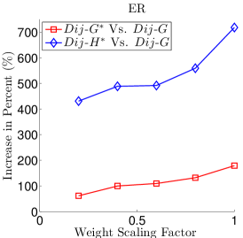
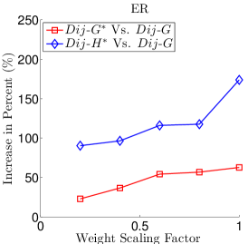
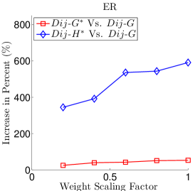
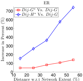
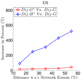
Figure 7: (a), (b) show ER increase for algorithms Dij-G^∗ and Dij-H^∗for Paris dataset for Settings $i$ and $ii$ respectively. (c), (d) show ER increase for algorithms Dij-G^∗ and Dij-H^∗for New York dataset for Settings $i$ and $ii$ respectively. (e), (f) show ER increase for algorithms Dij-G^∗ and Dij-H^∗for London dataset for Settings $i$ and $ii$ respectively.

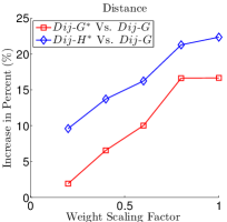
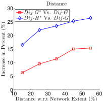
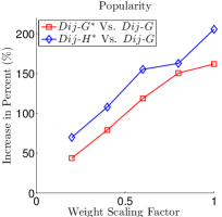
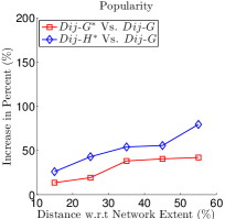
Figure 8: (a), (c) show Distance and Flickr popularity increase for algorithms Dij-G^∗ and Dij-H^∗ for Paris dataset for experimental Setting $i$. (b), (d) show Distance and Flickr popularity increase for algorithms Dij-G^∗ and Dij-H^∗ for Paris dataset for experimental Setting $ii$.

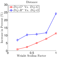
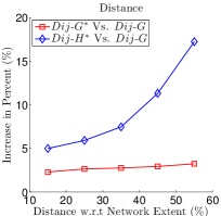
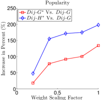
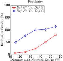
Figure 9: (a), (c) show Distance and Flickr popularity increase for algorithms Dij-G^∗ and Dij-H^∗ for New York dataset for experimental Setting $i$. (b), (d) show Distance and Flickr popularity increase for algorithms Dij-G^∗ and Dij-H^∗ for New York dataset for experimental Setting $ii$.

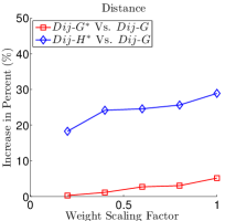
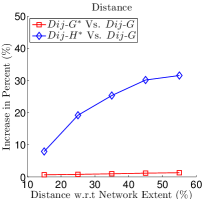
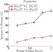
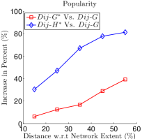
Figure 10: (a), (c) show Distance and Flickr popularity increase for algorithms Dij-G^∗ and Dij-H^∗ for London dataset for experimental Setting $i$. (b), (d) show Distance and Flickr popularity increase for algorithms Dij-G^∗ and Dij-H^∗ for London dataset for experimental Setting $ii$.

It is clear that Dij-G^∗ always performs better than Dij-H^∗ in terms of path length increase, but Dij-H^∗ performs always better in terms of ER and popularity. This is because Dij-H^∗ routes directly through the PoIs, causing greater detours, but passing along highly weighted parts of the enriched graph $G^{*}$, which mostly coincide with dense Flickr regions.

Continuing, in Setting $(ii)$ the full weights are taken into account, but the proportionate distance of start and target node w.r.t. the extent of the whole network is varied. We consider five different distance brackets of shortest path in the original graph $G$, the first one ranging from 10% to 20%, the last one ranging from 50% to 60% of the extent of the whole network. For 100 randomly chosen pairs of start and target nodes (within the respective distance bracket) paths with Dij-G , Dij-G^∗ and Dij-H^∗ are computed. As before, for each pair the difference w.r.t. ER, distance and popularity is computed and averaged out over all pairs. Figure 7 ((d), (e), (f)) show the increase of ER as we proceed through the distance brackets in all three datasets for the datasets of Paris, New York and London respectively. The increase in ER is in the range of 10% to 100% for Dij-G^∗ and in the range of 60% to 700% for Dij-H^∗. Figure 8, Figure 9 and Figure 10 ((b), (d)) show the results: As we proceed through the distance brackets, we observe an increase of the distance and popularity for Dij-G^∗ as well as Dij-H^∗ in comparison to Dij-G in all three datasets. The increase among all datasets, in terms of path length, is in the range of 1% to 15% for Dij-G^∗ and in the range of 5% to 25% for Dij-H^∗. Finally, the increase in terms of popularity is in the range of 5% to 60% for Dij-G^∗ and in the range of 30% to 120% for Dij-H^∗. As in our previous experimental setting, it is clear that Dij-G^∗ always outperforms Dij-H^∗ in terms of path length increase, while Dij-H^∗ always outperforms Dij-G^∗ in terms of enrichment ratio and popularity. The explanation for these results is, similarly with setting $i$, that Dij-H^∗ routes directly through the PoIs and therefore accumulates greater ER and higher popularity values.

Overall, we may conclude that both Dij-G^∗ and Dij-H^∗ show convincing results. Both algorithms yield significant increase in terms of ER as well as in terms of the independent Flickr-based measure popularity, while increasing path length only slightly. In the best case, ER increase amounts to 700% and 200% increase in terms of popularity (in comparison to the conventional shortest paths, as computed by Dij-G ), while the worst case increase in path length is only 25%. Consequently, we can claim that spatial relations, extracted from crowdsourced information, can indeed be used to enrich actual road networks and define an alternative kind of routing which reflects what people perceive as “close”.

Finally, Figure 11 illustrates the trade-off that we take by deviating from the shortest path in order to obtain more interesting paths. This figure shows the relative increase in distance and popularity of the paths returned by our proposed approaches Dij-G^∗ and Dij-H^∗, compared to the baseline approach Dij-G. For all three data sets, we can observe that using the Dij-G^∗ approach we can obtain a significant increase in popularity of up to $150\%$ for the meager price of no more than $10\%$ additional distance incurred. In contrast, using the Dij-H^∗ approach we get an even higher increase in popularity of the returned routes. However, this increase in popularity incurs a more significant distance overhead of up to $20\%$. In this experiments we used a scaling factor of $\alpha=0.5$. The trade-off between popularity and distance can be further balanced by adapting $\alpha$, as we have seen in Figures 8-10 ((a),(c)).

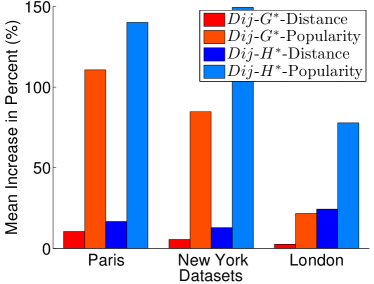
(a) Setting i

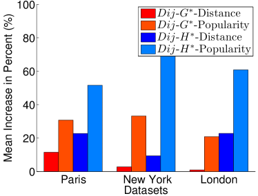
(b) Setting ii

Figure 11: Trade-off between distance and popularity of paths.

7 Conclusions and Outlook

In this work we presented an approach to computing knowledge-enriched paths within road networks. We incorporated and developed novel methods to extract spatial relations between pairs of Points of Interest such as “near” or “close by” from crowdsourced textual data, namely travel blogs. We quantified the extracted relations using probabilistic models to handle the inherent uncertainty of user-generated content. Based on these models, we proposed a new cost function to enrich real world road networks, reflecting the closeness aspect according to the crowd. In contrast to existing approaches, we did not enrich previously computed paths with semantical information, but the entire network. Continuing, two routing algorithms were presented taking this closeness aspect into account. Finally, we evaluated our ideas on three real world road network datasets, i.e., Paris, France, New York City, USA, and London, UK. We used metadata from geotagged Flickr photos as a ground truth to support our initial goal of providing more popular paths.

For future work, we are researching alternative methods for aggregating all categories of spatial relations. Furthermore, we would like to investigate ways to suggest the popular path descriptions to the user based on the Points of Interest they will encounter underway.

8 Appendix

The re-estimation of parameters $\lambda_{i}=\{w_{i},\mu_{i},\Sigma_{i}\}$ of a given GMM $p(d|\lambda)$ per each EM step, can be accomplished by the application of the following equations.

For all components $i\in\{1,...,M\}$

$$P(i|D_{j})=\frac{w_{i}g(D_{j};\lambda_{i})}{p(D_{j}|\lambda)}$$ (4)

$$w_{i}=\sum_{j=1}^{n}\frac{P(i|D_{j})}{n}$$ (5)

$$\mu_{i}=\sum_{j=1}^{n}\frac{P(i|D_{j})D_{j}}{nw_{i}}$$ (6)

$$\Sigma_{i}=\sum_{j=1}^{n}\frac{P(i|D_{j})(D_{j}-\mu_{i})(D_{j}-\mu_{i})^{\intercal}}{nw_{i}}$$ (7)

EM re-estimates model parameters $\lambda=(\lambda_{1},\dots,\lambda_{M})$ until the convergence of log-likelihood $\mathcal{L}$ given by Equation 1. As mentioned before, the EM algorithm is a greedy parameter estimation algorithm and is not guaranteed to lead us to the solution yielding maximum log-likelihood on $\mathcal{D}$ among all maxima of the log-likelihood. Nevertheless, using the EM algorithm, if we are “close” to the global optimum (maximum) of the parameter space, then it is very likely we can obtain the globally optimal solution.

References

- [1] L. O. Alvares, V. Bogorny, B. Kuijpers, J. A. F. de Macedo, B. Moelans, and A. Vaisman. A model for enriching trajectories with semantic geographical information. In Proc. of the 15th Annual ACM Int’l Symp. on Advances in Geographic Information Systems, pages 22:1–22:8, 2007.
- [2] C. M. Bishop. Pattern Recognition and Machine Learning (Information Science and Statistics). Springer-Verlag New York, Inc., Secaucus, NJ, USA, 2006.
- [3] A. P. Dempster, N. M. Laird, and D. B. Rubin. Maximum likelihood from incomplete data via the em algorithm. Journal of the Royal Statistical Society, Series B, 39(1):1–38, 1977.
- [4] M. Duckham and L. Kulik. Simplest paths: Automated route selection for navigation. In Spatial Information Theory. Foundations of Geographic Information Science, pages 169–185. 2003.
- [5] D. Feldman, A. Sugaya, C. Sung, and D. Rus. idiary: From gps signals to a text-searchable diary. In Proc. of the 11th ACM Conf. on Embedded Networked Sensor Systems, pages 6:1–6:12, 2013.
- [6] F. Graf, H.-P. Kriegel, M. Renz, and M. Schubert. Mario: Multi-attribute routing in open street map. In Advances in Spatial and Temporal Databases, pages 486–490. 2011.
- [7] S. Hansen, K.-F. Richter, and A. Klippel. Landmarks in openls — a data structure for cognitive ergonomic route directions. In M. Raubal, H. Miller, A. Frank, and M. Goodchild, editors, Geographic Information Science, volume 4197 of Lecture Notes in Computer Science, pages 128–144. Springer Berlin Heidelberg, 2006.
- [8] E. Loper and S. Bird. Nltk: The natural language toolkit. In Proc. of the ETMTNLP, pages 63–70, 2002.
- [9] M. Lv, L. Chen, and G. Chen. Discovering personally semantic places from gps trajectories. In Proc. of the 21st ACM CIKM, pages 1552–1556, 2012.
- [10] H. Mousselly-Sergieh, D. Watzinger, B. Huber, M. Döller, E. Egyed-Zsigmond, and H. Kosch. World-wide scale geotagged image dataset for automatic image annotation and reverse geotagging. In Proc. of the 5th ACM MMSys, pages 47–52, 2014.
- [11] A. T. Palma, V. Bogorny, B. Kuijpers, and L. O. Alvares. A clustering-based approach for discovering interesting places in trajectories. In Proc. of the ACM Symp. on Applied Computing, pages 863–868, 2008.
- [12] C. Parent, S. Spaccapietra, C. Renso, G. Andrienko, N. Andrienko, V. Bogorny, M. L. Damiani, A. Gkoulalas-Divanis, J. Macedo, N. Pelekis, Y. Theodoridis, and Z. Yan. Semantic trajectories modeling and analysis. ACM Comput. Surv. ’13, 45(4):42:1–42:32, Aug. 2013.
- [13] D. Quercia, R. Schifanella, and L. M. Aiello. The shortest path to happiness: Recommending beautiful, quiet, and happy routes in the city. CoRR, abs/1407.1031, 2014.
- [14] M. Raubal and S. Winter. Enriching wayfinding instructions with local landmarks. In Proceedings of the Second International Conference on Geographic Information Science, GIScience ’02, pages 243–259, London, UK, UK, 2002. Springer-Verlag.
- [15] D. Sacharidis and P. Bouros. Routing directions: Keeping it fast and simple. In Proc. of the 21st ACM SIGSPATIAL GIS, pages 164–173, 2013.
- [16] G. Skoumas, D. Pfoser, and A. Kyrillidis. On quantifying qualitative geospatial data: A probabilistic approach. In Proc. of the 2nd ACM GEOCROWD, pages 71–78, 2013.
- [17] S. Spaccapietra and C. Parent. Adding meaning to your steps. In Proc. of the 30th Int’l Conf. on Conceptual Modeling, pages 13–31, 2011.
- [18] J. J. Verbeek, N. Vlassis, and B. Kröse. Efficient greedy learning of gaussian mixture models. Neural Computation, 15:469–485, 2003.
- [19] M. Westphal and J. Renz. Evaluating and minimizing ambiguities in qualitative route instructions. In Proc. of the 19th ACM Int’l Conf. on Advances in Geographic Information Systems, pages 171–180, 2011.
- [20] Z. Yan, D. Chakraborty, C. Parent, S. Spaccapietra, and K. Aberer. Semitri: A framework for semantic annotation of heterogeneous trajectories. In Proc. of the 14th Int’l Conf. on Extending Database Technology, pages 259–270, 2011.
- [21] Z. Yan, D. Chakraborty, C. Parent, S. Spaccapietra, and K. Aberer. Semantic trajectories: Mobility data computation and annotation. ACM Trans. Intell. Syst. Technol., 4(3):49:1–49:38, July 2013.
- [22] Z. Yan, L. Spremic, D. Chakraborty, C. Parent, S. Spaccapietra, and K. Aberer. Automatic construction and multi-level visualization of semantic trajectories. In Proc. of the 18th Int’l Conf. on Advances in Geographic Information Systems, pages 524–525, 2010.