Fourier Theory on the Complex Plane I
Conjugate Pairs of Fourier Series
and Inner Analytic Functions

Abstract

A correspondence between arbitrary Fourier series and certain analytic functions on the unit disk of the complex plane is established. The expression of the Fourier coefficients is derived from the structure of complex analysis. The orthogonality and completeness relations of the Fourier basis are derived in the same way. It is shown that the limiting function of any Fourier series is also the limit to the unit circle of an analytic function in the open unit disk. An alternative way to recover the original real functions from the Fourier coefficients, which works even when the Fourier series are divergent, is thus presented. The convergence issues are discussed up to a certain point. Other possible uses of the correspondence established are pointed out.

1 Introduction

In this paper we will establish an interesting relation between Fourier series and analytic functions. This leads to an alternative way to deal with Fourier series and to characterize the corresponding real functions. This relation will allow us to discuss the convergence of Fourier series in terms of the convergence of the Taylor series of analytic functions. The convergence issues will be developed up to a certain point, and further developments will be discussed in a follow-up paper [1]. This relation will also give us an alternative way to recover, from the coefficients of the series, the functions that originated them, which works even if the Fourier series are divergent. Perhaps most importantly, it will provide a different and possibly richer point of view for Fourier series and the corresponding real functions.

We will use repeatedly the following very well-known and fundamental theorem of complex analysis, about complex power series [2]. If we consider the general complex power series written around the origin $z=0$,

$$S_{z}=\sum_{k=0}^{\infty}c_{k}z^{k},$$

where $z=x+\mbox{\boldmath$\imath$}y$ is a complex variable and $c_{k}$ are arbitrary complex constants, then the following holds. If $S_{z}$ converges at a point $z_{1}\neq 0$, then it is convergent and absolutely convergent on an open disk centered at $z=0$ with its boundary passing through $z_{1}$. In addition to this, it converges uniformly on any closed set contained within this open disk. We will refer to this state of affairs in what regards convergence as strong convergence, and will refer to this theorem as the basic convergence theorem. Furthermore, the power series converges to an analytic function of which it is the Taylor series around $z=0$.

We will make a conceptual distinction between trigonometric series and Fourier series. An arbitrary real trigonometric series on the real variable $\theta$ with domain in the periodic interval $[-\pi,\pi]$ is given by

$$S=\frac{1}{2}\,\alpha_{0}+\sum_{k=1}^{\infty}\alpha_{k}\cos(k\theta)+\sum_{k=1}^{\infty}\beta_{k}\sin(k\theta),$$

where $\alpha_{k}$ and $\beta_{k}$ are any real numbers. If there is a real function $f(\theta)$ such that the coefficients $\alpha_{k}$ and $\beta_{k}$ are given in terms of that function by the integrals

$$\alpha_{k} = \frac{1}{\pi}\int_{-\pi}^{\pi}d\theta\,f(\theta)\cos(k\theta),$$

$$\beta_{k} = \frac{1}{\pi}\int_{-\pi}^{\pi}d\theta\,f(\theta)\sin(k\theta),$$

then we call this series the Fourier series of that function [3]. Since the Fourier coefficients are defined by means of integrals, it is clear that one can add to $f(\theta)$ any zero-measure function without modifying them. This means that a convergent Fourier series can only be said to converge almost everywhere to the function which originated it, that is, with the possible exclusion of a zero-measure subset of the domain.

With this limitation, the Fourier basis in the space of real functions on the periodic interval, formed by the constant function, the set of functions $\cos(k\theta)$, with $k=1,\ldots,\infty$, and the set of functions $\sin(k\theta)$, with $k=1,\ldots,\infty$, is complete to generate all sufficiently well-behaved functions in that interval. With the exclusion of the constant function, the remaining basis generates the set of all sufficiently well-behaved zero-average real functions. The remaining basis functions satisfy the orthogonality relations

$$\frac{1}{\pi}\int_{-\pi}^{\pi}d\theta\,\cos(k_{1}\theta)\cos(k_{2}\theta) = \delta_{k_{1}k_{2}},$$

$$\frac{1}{\pi}\int_{-\pi}^{\pi}d\theta\,\sin(k_{1}\theta)\sin(k_{2}\theta) = \delta_{k_{1}k_{2}},$$

$$\frac{1}{\pi}\int_{-\pi}^{\pi}d\theta\,\cos(k_{1}\theta)\sin(k_{2}\theta) = 0,$$ (1)

for $k_{1}\geq 1$ and $k_{2}\geq 1$. In a stricter sense, the good-behavior conditions on the real functions are that they be integrable and that they be such that their Fourier series converge. However, one might consider the set of coefficients themselves to be sufficient to characterize the function that originated them, even if the series does not converge. This makes full sense if there is an alternative way to recover the functions from the coefficients of their series, such as the one we will present in this paper, which is not dependent on the convergence of the series. In this case the condition of integrability suffices. The important point to be kept in mind here is that the set of coefficients determines the function uniquely almost everywhere over the periodic interval.

The parity of the real functions will play an important role in this paper. Any real function defined in a symmetric domain around zero, without any additional hypotheses, can be separated into its even and odd parts. An even function is one that satisfies the condition $f(-\theta)=f(\theta)$, while an odd one satisfies the condition $f(-\theta)=-f(\theta)$. For any real function we can write that $f(\theta)=f_{\rm c}(\theta)+f_{\rm s}(\theta)$, with

$$f_{\rm c}(\theta) = \frac{f(\theta)+f(-\theta)}{2},$$

$$f_{\rm s}(\theta) = \frac{f(\theta)-f(-\theta)}{2},$$

where $f_{\rm c}(\theta)$ is even and $f_{\rm s}(\theta)$ is odd. The Fourier basis can also be separated into even and odd parts. Since the constant function and the cosines are even, they generate the even parts of the real functions, while the sines, being odd, generate the odd parts. Since the set of cosines and the set of sines are two independent and mutually orthogonal sets of functions, the convergence of the trigonometric series can only be accomplished by the separate convergence of the cosine sub-series and the sine sub-series, which we denote by

$$S_{\rm c} = \sum_{k=1}^{\infty}\alpha_{k}\cos(k\theta),$$

$$S_{\rm s} = \sum_{k=1}^{\infty}\beta_{k}\sin(k\theta),$$

so that $S=\alpha_{0}/2+S_{\rm c}+S_{\rm s}$. For simplicity, in this paper we will consider only series in which $\alpha_{0}=0$, which correspond to functions $f(\theta)$ that have zero average over the periodic interval. There is of course no loss of generality involved in doing this, since the addition of a constant term is a trivial procedure that does not bear on the convergence issues. The discussion of the convergence of arbitrary trigonometric series $S$ is therefore equivalent to the separate discussion of the convergence of arbitrary cosine series $S_{\rm c}$ and arbitrary sine series $S_{\rm s}$. These last two classes consist of trigonometric series with definite parities and we will name them Definite-Parity trigonometric series, or DP trigonometric series for short.

A note about the fact that we limit ourselves to real Fourier series here. We might as well consider the series $S$ with complex coefficients $\alpha_{k}$ and $\beta_{k}$, but due to the linearity of the series with respect to these coefficients, any such complex Fourier series would at once decouple into two real Fourier series, one in the real part and one in the imaginary part, and would therefore reduce the discussion to the one we choose to develop here. Therefore nothing fundamentally new is introduced by the examination of complex Fourier series, and it is enough to limit the discussion to the real case.

2 Trigonometric Series on the Complex Plane

First of all, let us establish a very basic correspondence between real trigonometric series and power series in the complex plane. In this section we do not assume that the trigonometric series are Fourier series. In fact, for the time being we impose no additional restrictions on the numbers $\alpha_{k}$ and $\beta_{k}$, other than that they be real, and in particular we do not assume anything about the convergence of the series.

Consider then an arbitrary DP trigonometric series. We now introduce a useful definition. Given a cosine series $S_{\rm c}$ with coefficients $\alpha_{k}$, we will define from it a corresponding sine series by

$$\bar{S}_{\rm c}=\sum_{k=1}^{\infty}\alpha_{k}\sin(k\theta).$$

We will call this new trigonometric series the Fourier-Conjugate series to $S_{\rm c}$, or the FC series for short. Note that $\bar{S}_{\rm c}$ is odd instead of even. Similarly, given a sine series $S_{\rm s}$ with coefficients $\beta_{k}$, we will define from it a corresponding cosine series by

$$\bar{S}_{\rm s}=\sum_{k=1}^{\infty}\beta_{k}\cos(k\theta),$$

which we will also name the Fourier-Conjugate series to $S_{\rm s}$. Note that $\bar{S}_{\rm s}$ is even instead of odd. We see therefore that the set of all DP trigonometric series can be organized in pairs of mutually conjugate series. In any given pair, each series is the FC series of the other.

From now on we will denote all trigonometric series coefficients by $a_{k}$, regardless of whether the series originally under discussion is a cosine series or a sine series. Now, given any cosine series $S_{\rm c}$ or any sine series $S_{\rm s}$, we may define from it a complex series $S_{v}$ by the use of the original series and its FC series as the real and imaginary parts of the complex series. In the case of an original cosine series we thus define

$$S_{v}=S_{\rm c}+\mbox{\boldmath$\imath$}\bar{S}_{\rm c},$$

while in the case of an original sine series we define

$$S_{v}=\bar{S}_{\rm s}+\mbox{\boldmath$\imath$}S_{\rm s}.$$

In this way the discussion of the convergence of arbitrary DP trigonometric series can be reduced to the discussion of the convergence of the corresponding complex series $S_{v}$. In either one of the two cases above this series may be written as

$$S_{v} = \sum_{k=1}^{\infty}a_{k}\cos(k\theta)+\mbox{\boldmath$\imath$}\sum_{k=1}^{\infty}a_{k}\sin(k\theta)$$

$$= \sum_{k=1}^{\infty}a_{k}\left[\cos(k\theta)+\mbox{\boldmath$\imath$}\sin(k\theta)\right],$$

where the coefficients $a_{k}$ are still completely arbitrary. If we now define the complex variable $v=\exp(\mbox{\boldmath$\imath$}\theta)$, then using Euler’s formula we may write this complex series as

$$S_{v}=\sum_{k=1}^{\infty}a_{k}v^{k},$$

so that it becomes, therefore, a complex power series with real coefficients on the unit circle centered at the origin, in the complex plane. Finally, we may look at this series as a restriction to the unit circle of a full power series on the complex plane if we introduce an extra real variable $\rho\geq 0$, so that a complex variable

$$z = \rho v$$

$$= \rho\,{\rm e}^{\mbox{\boldmath$\imath$}\theta}$$

can be defined over the whole complex plane, and consider the complex power series, still with real coefficients,

$$S_{z}=\sum_{k=1}^{\infty}a_{k}z^{k}.$$

This is a complex power series centered at $z=0$, with no $k=0$ term, so that is assumes the value zero at $z=0$. Apart from the fact that $a_{0}=0$, it has real but otherwise arbitrary coefficients. The series $S_{v}$ that we constructed from a pair of FC trigonometric series is just $S_{z}$ restricted to $\rho=1$, for $\theta\in[-\pi,\pi]$. In other words, the series $S_{v}$ is a restriction to the unit circle of the complex power series we just defined. There is, therefore, a one-to-one correspondence between pairs of mutually FC trigonometric series and complex power series around $z=0$ with real coefficients and $a_{0}=0$.

We thus establish that the discussion of the convergence of arbitrary DP trigonometric series can be reduced to the discussion of the convergence of the corresponding complex power series $S_{z}$ on the unit circle. In fact, the whole question of the convergence of trigonometric series is revealed to be identical to the question of the convergence of complex power series on the boundary of the unit disk, including the cases in which that disk is the maximum disk of convergence of the power series.

3 Fourier Series on the Complex Plane

Let us now show that the usual formulas giving the Fourier coefficients, in terms of integrals involving the corresponding real functions, follow as consequences of the analytic properties of certain complex functions within the open unit disk. In order to do this, let us consider a pair of FC trigonometric series that have the rather weak property that there is at least one value of $\theta$ for which both elements of the pair are convergent. Note that this constitutes an indirect restriction on the coefficients of the series. It follows at once that the power series $S_{z}$ converges at the point on the unit circle that corresponds to that value of $\theta$. Consequently, it follows from the basic convergence theorem that the power series is strongly convergent at least on the open unit disk. Furthermore, it converges to a complex function that is analytic at least on the open unit disk, which we will denote by $w(z)$, and therefore we may now write

$$w(z)=\sum_{k=1}^{\infty}a_{k}z^{k}.$$

Note that, since the coefficients are real, the function $w(z)$ reduces to a purely real function on the open interval $(-1,1)$ of the real axis. It is therefore the analytic continuation of a real analytic function defined on that interval. Apart from this fact, from the fact that $w(0)=0$, and from the fact that it is analytic on the open unit disk, it is an otherwise arbitrary analytic function. In addition to all this, we have that $S_{z}$ is the Taylor series of $w(z)$ around $z=0$. We will call an analytic function that has these properties an inner analytic function. Let us list the defining properties. An inner analytic function is one that:

• is analytic at least on the open unit disk;

• is the analytic continuation of a real function defined in $(-1,1)$;

• assumes the value zero at $z=0$.

Let us now examine another property of $w(z)$ implied by the fact that it is the analytic continuation of a real function. If we use polar coordinates and write $z=\rho\exp(\mbox{\boldmath$\imath$}\theta)$, with $\theta\in[-\pi,\pi]$, then we may write out the Taylor series of $w(z)$ as

$$w(z)=\sum_{k=1}^{\infty}a_{k}\rho^{k}\left[\cos(k\theta)+\mbox{\boldmath$\imath$}\sin(k\theta)\right].$$

Since the coefficients are real, we have at once that

$$w(z)=\left[\,\sum_{k=1}^{\infty}a_{k}\rho^{k}\cos(k\theta)\right]+\mbox{\boldmath$\imath$}\left[\,\sum_{k=1}^{\infty}a_{k}\rho^{k}\sin(k\theta)\right],$$

where the expressions within square brackets are real. If we write $w(z)$ in terms of its real and imaginary parts,

$$w(z)=f_{\rm c}(\rho,\theta)+\mbox{\boldmath$\imath$}f_{\rm s}(\rho,\theta),$$

then the real part $f_{\rm c}(\rho,\theta)$ must be even on $\theta$, because it is the function that the cosine series contained in $S_{z}$ converges to,

$$f_{\rm c}(\rho,\theta)=\sum_{k=1}^{\infty}a_{k}\rho^{k}\cos(k\theta).$$

Similarly, the imaginary part $f_{\rm s}(\rho,\theta)$ must be odd on $\theta$, because it is the function that the sine series contained in $S_{z}$ converges to,

$$f_{\rm s}(\rho,\theta)=\sum_{k=1}^{\infty}a_{k}\rho^{k}\sin(k\theta).$$

With these preliminaries established, we may now proceed towards our objective here, which consists of the inversion of the relations above, so that we may write $a_{k}$ in terms of $f_{\rm c}(\rho,\theta)$, or in terms of $f_{\rm s}(\rho,\theta)$, by means of the use of the analytic structure within the open unit disk. Consider then the Cauchy integral formulas for the function $w(z)$ and its derivatives, written around $z=0$ for the $k^{\rm th}$ derivative,

$$w^{k\prime}(0)=\frac{k!}{2\pi\mbox{\boldmath$\imath$}}\oint_{C}dz\,\frac{w(z)}{z^{k+1}},$$

where $C$ is the circle centered at $z=0$ with radius $\rho\in(0,1)$. The coefficients of the Taylor series of $w(z)$ may be written in terms of these integrals, so that we have for $a_{k}$

$$a_{k} = \frac{w^{k\prime}(0)}{k!}$$

$$= \frac{1}{2\pi\mbox{\boldmath$\imath$}}\oint_{C}dz\,\frac{w(z)}{z^{k+1}}.$$

It is very important to note that since $w(z)$ is analytic in the open unit disk, by the Cauchy-Goursat theorem the integral is independent of $\rho$ within that disk, and therefore so are the coefficients $a_{k}$. We now write the integral explicitly, using the integration variable $\theta$ on the circle of radius $\rho$. We have $dz=\mbox{\boldmath$\imath$}\rho\exp(\mbox{\boldmath$\imath$}\theta)d\theta$, and therefore get

$$a_{k} = \frac{1}{2\pi\mbox{\boldmath$\imath$}}\int_{-\pi}^{\pi}d\theta\,\mbox{\boldmath$\imath$}\rho^{-k}\,{\rm e}^{-\mbox{\boldmath$\imath$}k\theta}w(z)$$

$$= \frac{\rho^{-k}}{2\pi}\int_{-\pi}^{\pi}d\theta\,\left[f_{\rm c}(\rho,\theta)+\mbox{\boldmath$\imath$}f_{\rm s}(\rho,\theta)\right]\left[\cos(k\theta)-\mbox{\boldmath$\imath$}\sin(k\theta)\right]$$

$$= \frac{\rho^{-k}}{2\pi}\int_{-\pi}^{\pi}d\theta\,\left\{\rule{0.0pt}{10.76385pt}\left[f_{\rm c}(\rho,\theta)\cos(k\theta)+f_{\rm s}(\rho,\theta)\sin(k\theta)\right]\right.+$$

$$\hskip 60.00009pt+\left.\mbox{\boldmath$\imath$}\left[f_{\rm s}(\rho,\theta)\cos(k\theta)-f_{\rm c}(\rho,\theta)\sin(k\theta)\right]\rule{0.0pt}{10.76385pt}\right\}.$$

Since we know that $a_{k}$ are real, we may at once conclude that the imaginary part of this last integral is zero. But we can state more than just that, because all the functions appearing in all these integrals have definite parities on $\theta$, and hence we see that the integrands that appear in the imaginary part are odd, while the integrals are over symmetric intervals. We therefore conclude that the following two integrals are separately zero,

$$\int_{-\pi}^{\pi}d\theta\,f_{\rm s}(\rho,\theta)\cos(k\theta) = 0,$$

$$\int_{-\pi}^{\pi}d\theta\,f_{\rm c}(\rho,\theta)\sin(k\theta) = 0,$$

for all $k$. We are therefore left with the following expression for $a_{k}$,

$$a_{k}=\frac{\rho^{-k}}{2\pi}\int_{-\pi}^{\pi}d\theta\,\left[f_{\rm c}(\rho,\theta)\cos(k\theta)+f_{\rm s}(\rho,\theta)\sin(k\theta)\right].$$ (2)

In order to continue the analysis of the coefficients $a_{k}$ we consider now the following integral on the same circuit $C$,

$$\oint_{C}dz\,w(z)z^{k-1}=0,$$

with $k>0$. The integral is zero by the Cauchy-Goursat theorem, since for $k>0$ the integrand is analytic on the open unit disk. As before we write the integral on the circle of radius $\rho$ using the integration variable $\theta$, to get

$$0 = \int_{-\pi}^{\pi}d\theta\,\mbox{\boldmath$\imath$}\rho^{k}\,{\rm e}^{\mbox{\boldmath$\imath$}k\theta}w(z)$$

$$= \mbox{\boldmath$\imath$}\rho^{k}\int_{-\pi}^{\pi}d\theta\,\left[f_{\rm c}(\rho,\theta)+\mbox{\boldmath$\imath$}f_{\rm s}(\rho,\theta)\right]\left[\cos(k\theta)+\mbox{\boldmath$\imath$}\sin(k\theta)\right]$$

$$= \mbox{\boldmath$\imath$}\rho^{k}\int_{-\pi}^{\pi}d\theta\,\left\{\rule{0.0pt}{10.76385pt}\left[f_{\rm c}(\rho,\theta)\cos(k\theta)-f_{\rm s}(\rho,\theta)\sin(k\theta)\right]\right.+$$

$$\hskip 60.00009pt+\left.\mbox{\boldmath$\imath$}\left[f_{\rm s}(\rho,\theta)\cos(k\theta)+f_{\rm c}(\rho,\theta)\sin(k\theta)\right]\rule{0.0pt}{10.76385pt}\right\}.$$

Once again the integrals that appear in the imaginary part of this last expression are zero by parity arguments, and since $\rho\neq 0$ we are left with

$$\int_{-\pi}^{\pi}d\theta\,\left[f_{\rm c}(\rho,\theta)\cos(k\theta)-f_{\rm s}(\rho,\theta)\sin(k\theta)\right]=0,$$

which is valid for all $k>0$. We conclude therefore that the two integrals shown are equal,

$$\int_{-\pi}^{\pi}d\theta\,f_{\rm c}(\rho,\theta)\cos(k\theta)=\int_{-\pi}^{\pi}d\theta\,f_{\rm s}(\rho,\theta)\sin(k\theta),$$

for all $k>0$. If we now go back to the expression in Equation (2) for $a_{k}$ we see that the two integrals appearing in that expression are equal to each other. We may therefore write for the coefficients

$$a_{k} = \frac{\rho^{-k}}{\pi}\int_{-\pi}^{\pi}d\theta\,f_{\rm c}(\rho,\theta)\cos(k\theta)$$

$$= \frac{\rho^{-k}}{\pi}\int_{-\pi}^{\pi}d\theta\,f_{\rm s}(\rho,\theta)\sin(k\theta).$$

We observe now that these formulas for the coefficients $a_{k}$ are simple extensions of the usual formulas for the Fourier coefficients of the even function $f_{\rm c}(\rho,\theta)$ and the odd function $f_{\rm s}(\rho,\theta)$, and therefore are related in a simple way to the Fourier coefficients for the real function of $\theta$

$$f(\rho,\theta)=f_{\rm c}(\rho,\theta)+f_{\rm s}(\rho,\theta),$$

with $\rho$ interpreted as an extra parameter. In fact, these formulas become the usual ones in the $\rho\to 1$ limit, thus completing the construction of a pair of FC Fourier series on the unit circle.

Whether or not we may now take the limit $\rho\to 1$ in these formulas depends on whether or not the coefficients, and hence the integrals that define them, are continuous functions of $\rho$ at the unit circle, for limits coming from within the unit disk. We saw before that the coefficients are constant with $\rho$, and therefore are continuous functions of $\rho$ within the open unit disk. We therefore know that their $\rho\to 1$ limits exist. Furthermore, by construction these are the coefficients of the FC pair of DP trigonometric series we started with, on the unit circle. Therefore the coefficients assume at $\rho=1$ the values given by their limits when $\rho\to 1$.

Consequently, the coefficients $a_{k}$ and the expressions giving them within the open unit disk are continuous from within at the unit circle, as functions of $\rho$, and so are the integrals appearing in those expressions. We may now take the $\rho\to 1$ limit and therefore get the usual formulas for the Fourier coefficients,

$$a_{k} = \alpha_{k}$$

$$= \beta_{k},$$

$$\alpha_{k} = \frac{1}{\pi}\int_{-\pi}^{\pi}d\theta\,f_{\rm c}(1,\theta)\cos(k\theta),$$

$$\beta_{k} = \frac{1}{\pi}\int_{-\pi}^{\pi}d\theta\,f_{\rm s}(1,\theta)\sin(k\theta),$$

where

$$f_{\rm c}(1,\theta) = \lim_{\rho\to 1}f_{\rm c}(\rho,\theta),$$

$$f_{\rm s}(1,\theta) = \lim_{\rho\to 1}f_{\rm s}(\rho,\theta).$$

We see therefore that the two trigonometric series of the pair of FC series we started with, under the very weak hypothesis that they both converge at one common point, are in fact the DP Fourier series of the DP functions $f_{\rm c}(1,\theta)$ and $f_{\rm s}(1,\theta)$ which are obtained as the $\rho\to 1$ limits of the real part $f_{\rm c}(\rho,\theta)$ and of the imaginary part $f_{\rm s}(\rho,\theta)$ of the inner analytic function $w(z)$.

It is important to note that $w(z)$ might not be analytic at some points on the unit circle. Also, so far we cannot state that the Taylor series $S_{z}$ converges anywhere on the unit circle, besides that single point at which we assumed the convergence of the pair of FC trigonometric series. For it to be possible to define the real integrals over the unit circle, the $\rho\to 1$ limits of the functions $f_{\rm c}(\rho,\theta)$ and $f_{\rm s}(\rho,\theta)$ must exist at least almost everywhere on the unit circle parametrized by $\theta$. They may fail to exist at points where $w(z)$ has isolated singularities on that circle. Therefore, for the moment the definition of the trigonometric series as Fourier series on the unit circle must remain conditioned to the existence of these limits almost everywhere.

Note that, if the limits to the unit circle result in isolated singularities in $f_{\rm c}(1,\theta)$ or $f_{\rm s}(1,\theta)$, then these must be integrable ones along the unit circle, since the $a_{k}$ coefficients are all finite.

4 Fourier-Taylor Correspondence

Let us now show that there is a complete one-to-one correspondence between arbitrarily given pairs of real FC Fourier series and the inner analytic functions within the open unit disk. To this end, let us imagine that one begins the whole argument of the last section over again, but this time starting with a pair of FC Fourier series. What this means is that there is a zero-average real function $f(\theta)$ defined in the periodic interval such that the coefficients $a_{k}$ are given in terms of that function by the integrals

$$a_{k} = \frac{1}{\pi}\int_{-\pi}^{\pi}d\theta\,f_{\rm c}(\theta)\cos(k\theta)$$ (3)

$$= \frac{1}{\pi}\int_{-\pi}^{\pi}d\theta\,f_{\rm s}(\theta)\sin(k\theta),$$

where we have $f(\theta)=f_{\rm c}(\theta)+f_{\rm s}(\theta)$, with $f_{\rm c}(\theta)$ even on $\theta$ and $f_{\rm s}(\theta)$ odd on $\theta$. The two Fourier series generated by $f_{\rm c}(\theta)$ and $f_{\rm s}(\theta)$ have exactly the same coefficients, and are therefore the FC series of one another. We may therefore consider the corresponding functions to be FC functions of one another as well, even if the series do not converge. We will denote these FC functions by $\bar{f}_{\rm c}(\theta)$ in the case of an original cosine series with coefficients given by $f_{\rm c}(\theta)$, and by $\bar{f}_{\rm s}(\theta)$ in the case of an original sine series with coefficients given by $f_{\rm s}(\theta)$. We have therefore that

$$f_{\rm c}(\theta) = \bar{f}_{\rm s}(\theta),$$

$$f_{\rm s}(\theta) = \bar{f}_{\rm c}(\theta).$$

Note that $\bar{f}_{\rm c}(\theta)$ is in fact odd instead of even, while $\bar{f}_{\rm s}(\theta)$ is in fact even instead of odd.

As before, we assume that there is at least one value of $\theta$ for which both series in the FC pair converge. We may then use the coefficients $a_{k}$ to define the inner analytic function $w(z)$, as we did in the previous section, we may identify these coefficients as those of its Taylor series, and therefore these same coefficients turn out to be given by

$$a_{k} = \frac{\rho^{-k}}{\pi}\int_{-\pi}^{\pi}d\theta\,f_{\rm c}(\rho,\theta)\cos(k\theta)$$

$$= \frac{\rho^{-k}}{\pi}\int_{-\pi}^{\pi}d\theta\,f_{\rm s}(\rho,\theta)\sin(k\theta),$$

where $f_{\rm c}(\rho,\theta)$ and $f_{\rm s}(\rho,\theta)$ are respectively the real and imaginary parts of $w(z)$. Since the coefficients $a_{k}$ are in fact independent of $\rho$ in this last set of expressions, for $0<\rho<1$, and by construction have the same values as those given by the previous set of expressions, in Equation (3), which define them as Fourier coefficients of $f(\theta)$, we see that they are continuous from within as functions of $\rho$ in the limit $\rho\to 1$, which we may then take.

According to the results of the previous section, we conclude therefore that the two FC Fourier series we started with in this section are in fact the DP Fourier series of the functions $f_{\rm c}(\rho,\theta)$ and $f_{\rm s}(\rho,\theta)$ in the $\rho\to 1$ limit. Since the coefficients uniquely identify the function almost everywhere, as discussed in the introduction, we may now identify these two functions in the $\rho\to 1$ limit with the two functions $f_{\rm c}(\theta)$ and $f_{\rm s}(\theta)$ from which the coefficients $a_{k}$ were obtained in the first place, on the unit circle. We conclude that the limits

$$f_{\rm c}(\theta) = \lim_{\rho\to 1}f_{\rm c}(\rho,\theta),$$

$$f_{\rm s}(\theta) = \lim_{\rho\to 1}f_{\rm s}(\rho,\theta),$$

exist and hold almost everywhere over the unit circle. We may consider the $\rho\to 1$ limits of the functions $f_{\rm c}(\rho,\theta)$ and $f_{\rm s}(\rho,\theta)$ to be the maximally smooth members of sets of functions that are zero-measure equivalent and lead to the same set of Fourier coefficients. The functions $f_{\rm c}(\rho,\theta)$ and $f_{\rm s}(\rho,\theta)$, which according to our definitions are the Fourier Conjugate functions of each other, are also known as Harmonic Conjugate functions [4], since they are the real and imaginary parts of an analytic function, and hence are both harmonic functions on the real plane. They can be obtained from one another by the Hilbert transform [5]. In the $\rho\to 1$ limit we may also get functions $f_{\rm c}(\theta)$ and $f_{\rm s}(\theta)$ which are restriction to the unit circle of Harmonic Conjugate functions, if the function $w(z)$ is analytic at the limiting point. But in any case they are Fourier Conjugate to each other.

Up to this point we have established that every given pair of FC Fourier series, obtained from a given pair of FC real functions, such that both converge together on at least one point on the unit circle, corresponds to a specific inner analytic function, whose Taylor series converges on at least that point in the unit circle, and which reproduces the original pair of FC real function almost everywhere when one takes the $\rho\to 1$ limit from within the open unit disk to the unit circle.

Furthermore, we also see that we may work this argument in reverse. In other words, given an arbitrary inner analytic function $w(z)$ whose Taylor series converges on at least one point in the unit circle and which is well-defined almost everywhere over that circle, we may construct from it the DP Fourier series of two related functions. These two DP Fourier series are just the real and imaginary parts of the Taylor series of the analytic function $w(z)$, in the $\rho\to 1$ limit. Finally, since the coefficients $a_{k}$ are continuous functions of $\rho$ from within at the unit disk, and since the $S_{z}$ series converges on at least one point on the unit circle, we may also conclude that the two corresponding FC Fourier series converge together on that point of the unit circle.

This completes the establishment of a one-to-one correspondence between, on the one hand, pairs of real FC Fourier series that converge together on at least a single point of the periodic interval and, on the other hand, inner analytic functions that converge on at least one point of the unit circle and are well-defined almost everywhere over that circle. Note, however, that the analytic side of this correspondence is the more powerful one, because given the Fourier coefficients $a_{k}$ we may be able to define a convergent power series $S_{z}$ and thus an inner analytic function $w(z)$ even if the corresponding Fourier series diverge everywhere on the periodic interval.

This correspondence can be a useful tool, as it may make it easier to determine the convergence or lack thereof of given Fourier series. It may also be used to recover from the coefficients $a_{k}$ the function which generates a given Fourier series, even if that series is divergent. The way to do this is simply to determine the corresponding inner analytic function and then calculate the $\rho\to 1$ limit of the real and imaginary parts of that function. In Appendix C we will give a few simple examples of this type of procedure.

5 The Orthogonality Relations

The two most central elements of the structure of Fourier theory are the set of orthogonality relations and the completeness relation. Let us then show that these also follow from the structure of complex analysis. We start with the orthogonality relations, which we already gave in Equation (1) of the introduction. Of course the integrals involved are simple ones, and can be calculated by elementary means. Our objective here, however, is not to just calculate them but to show that they are a consequence of the analytic structure of the complex plane. We can do this by simply considering the Cauchy integral formulas for the coefficients $a_{k^{\prime}}$ of the Taylor series of a simple power $z^{k}$, with $k\geq 0$,

$$a_{k^{\prime}} = \frac{1}{k!}\,\frac{d^{k^{\prime}}z^{k}}{dz^{k^{\prime}}}(0)$$

$$= \frac{1}{2\pi\mbox{\boldmath$\imath$}}\oint_{C}dz\,\frac{z^{k}}{z^{k^{\prime}+1}},$$

where $C$ is a circle or radius $\rho$ centered at the origin, with $0<\rho\leq 1$. On the one hand, if $k^{\prime}>k$ we get $a_{k^{\prime}}=0$ due to the multiple differentiation of the power function, which is differentiated more times than the power itself. On the other hand, if $k^{\prime}<k$ we get $a_{k^{\prime}}=0$ when we calculate the derivatives and apply the result at zero, since in this case there is always at least one factor of $z$ left, or alternatively due to the Cauchy-Goursat theorem, because in this case the integrand is analytic and thus the integral is zero. If $k^{\prime}=k$, however, we get $a_{k^{\prime}}=1$, which we can get either directly from the result of the differentiation, or from the fact that in this case the integral is given by

$$\oint_{C}dz\,\frac{1}{z}=2\pi\mbox{\boldmath$\imath$},$$

as one can easily verify, either directly or by the residues theorem. In any case we get the result

$$\frac{1}{2\pi\mbox{\boldmath$\imath$}}\oint_{C}dz\,\frac{z^{k}}{z^{k^{\prime}+1}}=\delta_{kk^{\prime}}.$$

We now write the integral explicitly on the circle of radius $\rho$, using $\theta$ as the integration variable, with $z=\rho\exp(\mbox{\boldmath$\imath$}\theta)$ and thus with $dz=\mbox{\boldmath$\imath$}zd\theta$,

$$\delta_{kk^{\prime}} = \frac{1}{2\pi\mbox{\boldmath$\imath$}}\int_{-\pi}^{\pi}d\theta\,\mbox{\boldmath$\imath$}\,\rho^{k}\,{\rm e}^{\mbox{\boldmath$\imath$}k\theta}\rho^{-k^{\prime}}\,{\rm e}^{-\mbox{\boldmath$\imath$}k^{\prime}\theta}$$

$$= \frac{\rho^{k-k^{\prime}}}{2\pi}\int_{-\pi}^{\pi}d\theta\,\left[\cos(k\theta)+\mbox{\boldmath$\imath$}\sin(k\theta)\right]\left[\cos(k^{\prime}\theta)-\mbox{\boldmath$\imath$}\sin(k^{\prime}\theta)\right]$$

$$= \frac{\rho^{k-k^{\prime}}}{2\pi}\left\{\left[\int_{-\pi}^{\pi}d\theta\,\cos(k\theta)\cos(k^{\prime}\theta)+\int_{-\pi}^{\pi}d\theta\,\sin(k\theta)\sin(k^{\prime}\theta)\right]\right.+$$

$$\hskip 35.00005pt+\left.\mbox{\boldmath$\imath$}\left[\int_{-\pi}^{\pi}d\theta\,\sin(k\theta)\cos(k^{\prime}\theta)-\int_{-\pi}^{\pi}d\theta\,\cos(k\theta)\sin(k^{\prime}\theta)\right]\right\}.$$

One can see that the integrals in the imaginary part are zero due to parity arguments. In fact, these constitute some of the orthogonality relations, those including sines and cosines. We are left with

$$\delta_{kk^{\prime}}=\frac{\rho^{k-k^{\prime}}}{2\pi}\left[\int_{-\pi}^{\pi}d\theta\,\cos(k\theta)\cos(k^{\prime}\theta)+\int_{-\pi}^{\pi}d\theta\,\sin(k\theta)\sin(k^{\prime}\theta)\right].$$ (4)

For $k=0=k^{\prime}$ the second term vanishes, and the equation becomes a simple identity, which is in fact one of the other orthogonality relations. If, on the other hand, we have $k+k^{\prime}>0$, we now consider the integral, on the same circuit,

$$\oint_{C}dz\,z^{k}z^{k^{\prime}-1}=0,$$

which is zero due to the Cauchy-Goursat theorem, since the integrand is analytic within the circle $C$ for $k+k^{\prime}\geq 1$. Writing the integral explicitly on the circle we get

$$0 = \int_{-\pi}^{\pi}d\theta\,\mbox{\boldmath$\imath$}\,\rho^{k}\,{\rm e}^{\mbox{\boldmath$\imath$}k\theta}\rho^{k^{\prime}}\,{\rm e}^{\mbox{\boldmath$\imath$}k^{\prime}\theta}$$

$$= \mbox{\boldmath$\imath$}\rho^{k+k^{\prime}}\int_{-\pi}^{\pi}d\theta\,\left[\cos(k\theta)+\mbox{\boldmath$\imath$}\sin(k\theta)\right]\left[\cos(k^{\prime}\theta)-\mbox{\boldmath$\imath$}\sin(k^{\prime}\theta)\right]$$

$$= \mbox{\boldmath$\imath$}\rho^{k+k^{\prime}}\left\{\left[\int_{-\pi}^{\pi}d\theta\,\cos(k\theta)\cos(k^{\prime}\theta)-\int_{-\pi}^{\pi}d\theta\,\sin(k\theta)\sin(k^{\prime}\theta)\right]\right.+$$

$$\hskip 35.00005pt+\left.\mbox{\boldmath$\imath$}\left[\int_{-\pi}^{\pi}d\theta\,\sin(k\theta)\cos(k^{\prime}\theta)+\int_{-\pi}^{\pi}d\theta\,\cos(k\theta)\sin(k^{\prime}\theta)\right]\right\}.$$

Once again the integrals in the imaginary part are zero by parity arguments, and thus we are left with

$$\int_{-\pi}^{\pi}d\theta\,\cos(k\theta)\cos(k^{\prime}\theta)=\int_{-\pi}^{\pi}d\theta\,\sin(k\theta)\sin(k^{\prime}\theta),$$

since $\rho\neq 0$. If we now go back to our previous expression in Equation (4) we see that the two integrals that appear there are equal to each other, so we may write that

$$\frac{1}{\pi}\int_{-\pi}^{\pi}d\theta\,\cos(k\theta)\cos(k^{\prime}\theta) = \rho^{k^{\prime}-k}\delta_{kk^{\prime}}$$

$$= \delta_{kk^{\prime}},$$

$$\frac{1}{\pi}\int_{-\pi}^{\pi}d\theta\,\sin(k\theta)\sin(k^{\prime}\theta) = \rho^{k^{\prime}-k}\delta_{kk^{\prime}}$$

$$= \delta_{kk^{\prime}},$$

where the factor involving $\rho$ is irrelevant since the right-hand sides are only different from zero if $k=k^{\prime}$. We get therefore the complete set of orthogonality relations

$$\frac{1}{\pi}\int_{-\pi}^{\pi}d\theta\,\cos(k\theta)\cos(k^{\prime}\theta) = \delta_{kk^{\prime}},$$

$$\frac{1}{\pi}\int_{-\pi}^{\pi}d\theta\,\sin(k\theta)\sin(k^{\prime}\theta) = \delta_{kk^{\prime}},$$

$$\frac{1}{\pi}\int_{-\pi}^{\pi}d\theta\,\cos(k\theta)\sin(k^{\prime}\theta) = 0,$$

for $k\geq 1$ and $k^{\prime}\geq 1$, which are the relevant values for DP Fourier series. It is interesting to note that the orthogonality relations are valid on the circle of radius $\rho$ with $0<\rho\leq 1$, without the need to actually take the $\rho\to 1$ limit. We thus get a bit more than we bargained for in this case, for it would have been sufficient to establish these relation only on the unit circle. Note that this is different from what happened during the calculation of the coefficients of the Fourier series. However, in both cases the results come from the Cauchy integral formulas and the Cauchy-Goursat theorem, and in either case the same real integral appears, defining the usual scalar product in the space of real functions on the periodic interval.

6 The Completeness Relation

Let us now show that the completeness relation of the Fourier basis also follows from the structure of complex analysis. In order to do this, we must first show that the Dirac delta “function” can be represented in terms of the analytic structure within the open unit disk. We denote the Dirac delta “function” centered at $\theta=\theta_{1}$ on the unit circle by $\delta(\theta-\theta_{1})$. The definition of this mathematical object is that it is a symbolic representation of a limiting process which has the following four properties:

1. $\delta(\theta-\theta_{1})$ tends to zero when one takes the defining limit with $\theta\neq\theta_{1}$;

2. $\delta(\theta-\theta_{1})$ diverges to positive infinity when one takes the defining limit with $\theta=\theta_{1}$;

3. in the defining limit the integral

   $$\int_{a}^{b}d\theta\,\delta(\theta-\theta_{1})=1,$$

   has the value shown, for any interval $(a,b)$ which contains the point $\theta_{1}$;

4. given any continuous function $g(\theta)$, in the defining limit the integral

   $$\int_{a}^{b}d\theta\,g(\theta)\delta(\theta-\theta_{1})=g(\theta_{1}),$$

   has the value shown, for any interval $(a,b)$ which contains the point $\theta_{1}$.

Of course no real function exists that can have all these properties, which justifies the quotes in which we wrap the word “function” when referring to it. In order to construct the Dirac delta “function” we must first give an object or set of objects over which the limiting process can be defined, and then define that limiting process. In order to fulfill this program, we consider the complex function given within the open unit disk by

$$w_{\delta}(z)=\frac{1}{2\pi}-\frac{1}{\pi}\,\frac{z}{z-z_{1}},$$

as well as its restrictions to circles of radius $\rho$ centered at the origin, with $0<\rho<1$, where $z=\rho\exp(\mbox{\boldmath$\imath$}\theta)$ and where $z_{1}=\exp(\mbox{\boldmath$\imath$}\theta_{1})$ is a point on the unit circle. This function is analytic within the open unit disk, but it is not an inner analytic function, because $w_{\delta}(0)$ is not zero. However, we may write it in terms of another function $w(z)$ as

$$w_{\delta}(z) = \frac{1}{2\pi}+w(z),$$

$$w(z) = -\,\frac{1}{\pi}\,\frac{z}{z-z_{1}}.$$

Strictly speaking, $w(z)$ is not an inner analytic function either, because it does not reduce to a real function over the real axis. However, it does reduce to a real function over the straight line $z=\chi z_{1}$, with real $\chi$, since in this case we have

$$w(z)=-\,\frac{1}{\pi}\,\frac{\chi}{\chi-1}.$$

We see therefore that $w(z)$ is an inner analytic function rotated around the origin by the angle $\theta_{1}$ associated to $z_{1}$. Therefore this is just a simple extension of the structure we defined here. The limiting process to be used for the definition is just the $\rho\to 1$ limit to the unit circle. We will now show that the real part of $w_{\delta}(z)$, taken on the $\rho\to 1$ limit, satisfies all the required properties defining the Dirac delta “function”. In order to recover the real and imaginary parts of this complex function, we must now rationalize it,

$$w_{\delta}(z) = \frac{1}{2\pi}-\frac{1}{\pi}\,\frac{z(z^{*}-z_{1}^{*})}{(z-z_{1})(z^{*}-z_{1}^{*})}$$

$$= \frac{1}{2\pi}-\frac{1}{\pi}\,\frac{\left(\rho^{2}-zz_{1}^{*}\right)}{\rho^{2}-(zz_{1}^{*}+z^{*}z_{1})+1}$$

$$= \frac{1}{2\pi}-\frac{1}{\pi}\,\frac{\rho^{2}-\rho\cos(\Delta\theta)-\mbox{\boldmath$\imath$}\rho\sin(\Delta\theta)}{\rho^{2}-2\rho\cos(\Delta\theta)+1},$$

where $\Delta\theta=\theta-\theta_{1}$. We now examine the real part of this function,

$$\Re[w_{\delta}(z)]=\frac{1}{2\pi}-\frac{1}{\pi}\,\frac{\rho\left[\rho-\cos(\Delta\theta)\right]}{\left(\rho^{2}+1\right)-2\rho\cos(\Delta\theta)}.$$

If we now take the limit $\rho\to 1$, under the assumption that $\Delta\theta\neq 0$, we get

$$\lim_{\rho\to 1}\Re[w_{\delta}(z)] = \frac{1}{2\pi}-\frac{1}{\pi}\,\frac{1-\cos(\Delta\theta)}{2-2\cos(\Delta\theta)}$$

$$= \frac{1}{2\pi}-\frac{1}{2\pi}$$

$$= 0,$$

which is the correct value for the case of the Dirac delta “function”. Thus we see that the first property holds.

If, on the other hand, we calculate $\Re[w_{\delta}(z)]$ for $\Delta\theta=0$ and $\rho<1$ we obtain

$$\Re[w_{\delta}(z)] = \frac{1}{2\pi}-\frac{1}{\pi}\,\frac{\rho(\rho-1)}{(\rho-1)^{2}}$$

$$= \frac{1}{2\pi}-\frac{1}{\pi}\,\frac{\rho}{\rho-1},$$

which diverges to positive infinity as $\rho\to 1$ from below, as it should in order to represent the singular Dirac delta “function”. This establishes that the second property holds.

We then calculate the integral of $\Re[w_{\delta}(z)]$ over the circle of radius $\rho<1$, which is given by

$$I_{1} = \frac{1}{2\pi}\int_{-\pi}^{\pi}d\theta\,\rho\left\{1-\frac{2\rho\left[\rho-\cos(\Delta\theta)\right]}{\left(\rho^{2}+1\right)-2\rho\cos(\Delta\theta)}\right\}$$

$$= \frac{\rho}{2\pi}\int_{-\pi}^{\pi}d\theta\,\frac{\left(1-\rho^{2}\right)}{\left(\rho^{2}+1\right)-2\rho\cos(\Delta\theta)}$$

$$= \frac{\left(1-\rho^{2}\right)}{4\pi}\int_{-\pi}^{\pi}d\theta\,\frac{1}{\left[\left(\rho^{2}+1\right)/(2\rho)\right]-\cos(\Delta\theta)},$$

since $d(\Delta\theta)=d\theta$. Note that this is not the integral of an analytic function over a closed contour, but the integral of a real function over the circle of radius $\rho$. This real integral over $\theta$ can be calculated by residues. We introduce an auxiliary complex variable $\xi=\lambda\exp(\mbox{\boldmath$\imath$}\Delta\theta)$, which becomes simply $\exp(\mbox{\boldmath$\imath$}\Delta\theta)$ on the unit circle $\lambda=1$. We have $d\xi=\mbox{\boldmath$\imath$}\xi d\theta$, and so we may write the integral as

$$\int_{-\pi}^{\pi}d\theta\,\frac{1}{\left[\left(1+\rho^{2}\right)/(2\rho)\right]-\cos(\Delta\theta)} = \oint_{C}d\xi\,\frac{1}{\mbox{\boldmath$\imath$}\xi}\,\frac{2}{\left[\left(1+\rho^{2}\right)/\rho\right]-\xi-1/\xi}$$

$$= 2\mbox{\boldmath$\imath$}\oint_{C}d\xi\,\frac{1}{1-\left[\left(1+\rho^{2}\right)/\rho\right]\xi+\xi^{2}},$$

where the integral is now over the unit circle $C$ in the complex $\xi$ plane. The two roots of the quadratic polynomial on $\xi$ in the denominator are given by

$$\xi_{+} = 1/\rho,$$

$$\xi_{-} = \rho.$$

Since $\rho<1$, only the pole corresponding to $\xi_{-}$ lies inside the integration contour, so we get for the integral

$$\int_{-\pi}^{\pi}d\theta\,\frac{1}{\left[\left(1+\rho^{2}\right)/(2\rho)\right]-\cos(\Delta\theta)} = 2\mbox{\boldmath$\imath$}(2\pi\mbox{\boldmath$\imath$})\lim_{\xi\to\rho}\frac{1}{\xi-1/\rho}$$

$$= 4\pi\,\frac{\rho}{\left(1-\rho^{2}\right)}.$$

It follows that we have for the integral $I_{1}$

$$I_{1} = \frac{\left(1-\rho^{2}\right)}{4\pi\rho}\,4\pi\,\frac{\rho}{\left(1-\rho^{2}\right)}$$

$$= 1,$$

independently of $\rho$, including therefore the $\rho\to 1$ limit. Once we have this result, and since the integrand goes to zero everywhere on the unit circle except at $\Delta\theta=0$, which means that $\theta=\theta_{1}$, the integral can be changed to one over any open interval on the unit circle containing the point $\theta_{1}$, without any change in its limiting value. This establishes that the third property holds.

In order to establish the fourth and last property, we take an essentially arbitrary inner analytic function $\gamma(z)$, with the single additional restriction that it be well-defined at the point $z_{1}$, in the sense that its $\rho\to 1$ limit exists at $z_{1}$. This inner analytic function corresponds to a pair of FC real functions on the unit circle, both of which are well-defined at $z_{1}$. We now consider the following integral over the circle of radius $\rho<1$,

$$I_{2} = \frac{1}{2\pi}\int_{-\pi}^{\pi}d\theta\,\rho\,\gamma(z)\left\{1-\frac{2\rho\left[\rho-\cos(\Delta\theta)\right]}{\left(\rho^{2}+1\right)-2\rho\cos(\Delta\theta)}\right\}$$

$$= \frac{\rho}{2\pi}\int_{-\pi}^{\pi}d\theta\,\gamma(z)\,\frac{\left(1-\rho^{2}\right)}{\left(\rho^{2}+1\right)-2\rho\cos(\Delta\theta)}$$

$$= \frac{\left(1-\rho^{2}\right)}{4\pi}\int_{-\pi}^{\pi}d\theta\,\frac{\gamma(z)}{\left[\left(\rho^{2}+1\right)/(2\rho)\right]-\cos(\Delta\theta)},$$

since $d(\Delta\theta)=d\theta$. Note once more that this is not the integral of an analytic function over a closed contour, but two integrals of real functions, given by the real and imaginary parts of $\gamma(z)$, over the circle of radius $\rho$. These real integrals over $\theta$ can be calculated by residues, exactly like the one which appeared before in the case of $I_{1}$. The calculation is exactly the same except for the extra factor of $\gamma(z)$ to be taken into consideration when calculating the residue, so that we may write directly that

$$\int_{-\pi}^{\pi}d\theta\,\frac{\gamma(z)}{\left[\left(\rho^{2}+1\right)/(2\rho)\right]-\cos(\Delta\theta)} = 2\mbox{\boldmath$\imath$}(2\pi\mbox{\boldmath$\imath$})\lim_{\xi\to\rho}\frac{\gamma(z)}{\xi-1/\rho}$$

$$= 4\pi\,\frac{\rho}{\left(1-\rho^{2}\right)}\lim_{\xi\to\rho}\gamma(z).$$

Note now that since $\xi=\lambda\exp(\mbox{\boldmath$\imath$}\Delta\theta)$ and we must take the limit $\xi\to\rho$, we in fact have that in that limit

$$\lambda\,{\rm e}^{\mbox{\boldmath$\imath$}\Delta\theta}=\rho,$$

which implies that $\lambda=\rho$ and that $\Delta\theta=0$. We must therefore write $\gamma(z)$ at the point given by $\rho$ and $\Delta\theta=0$, that is, at the point given by $\rho$ and $\theta_{1}$,

$$\int_{-\pi}^{\pi}d\theta\,\frac{\gamma(z)}{\left[\left(\rho^{2}+1\right)/(2\rho)\right]-\cos(\Delta\theta)}=4\pi\,\frac{\rho}{\left(1-\rho^{2}\right)}\,\gamma(\rho,\theta_{1}).$$

It follows that we have for the integral $I_{2}$

$$I_{2} = \frac{\left(1-\rho^{2}\right)}{4\pi\rho}\,4\pi\,\frac{\rho}{\left(1-\rho^{2}\right)}\,\gamma(\rho,\theta_{1})$$

$$= \gamma(\rho,\theta_{1}).$$

Finally, we may now take the $\rho\to 1$ limit, since $\gamma(\rho,\theta)$ is well-defined in that limit, and thus obtain

$$\lim_{\rho\to 1}I_{2}=\gamma(1,\theta_{1}).$$

Once we have this result, and since the integrand goes to zero everywhere on the unit circle except at $\Delta\theta=0$, which means that $\theta=\theta_{1}$, the integral can be changed to one over any open interval on the unit circle containing the point $\theta_{1}$, without any change in its value. This establishes that the fourth and last property holds. We may then write symbolically that

$$\delta(\theta-\theta_{1})=\lim_{\rho\to 1}\Re[w_{\delta}(z)].$$

Note that in order to obtain this result it was not necessary to assume that $\gamma(z)$ is continuous at $z_{1}$ in the direction of $\theta$ along the unit circle. It was necessary to assume only that $\gamma(z)$ is continuous as a function of $\rho$, in the direction perpendicular to the unit circle. One can see therefore that, once more, we get a bit more than we bargained for, because we were able to establish the result with slightly weaker hypotheses than at first expected.

We are now in a position to establish the completeness relation using this representation of the Dirac delta “function”. If we use once again the Cauchy integral formulas for $w(z)$ we get for the coefficients of the Taylor expansion of $w(z)$

$$a_{k} = \frac{1}{2\pi\mbox{\boldmath$\imath$}}\oint_{C}dz\,\frac{w(z)}{z^{k+1}}$$

$$= \frac{1}{2\pi^{2}\mbox{\boldmath$\imath$}}\oint_{C}dz\,\frac{1}{z^{k}}\,\frac{(-1)}{z-z_{1}},$$

for $k\geq 1$, since $w(z)$ is a rotated inner analytic function. We now observe that the second ratio in the integrand can be understood as the sum of a geometric series, which is convergent so long as $\rho<1$,

$$\frac{(-1)}{z-z_{1}}=\frac{1}{z_{1}}\sum_{n=0}^{\infty}\left(\frac{z}{z_{1}}\right)^{n},$$

so that we may now write

$$a_{k} = \frac{1}{2\pi^{2}\mbox{\boldmath$\imath$}}\oint_{C}dz\,\frac{1}{z^{k}}\,\frac{1}{z_{1}}\sum_{n=0}^{\infty}\left(\frac{z}{z_{1}}\right)^{n}$$

$$= \frac{1}{2\pi^{2}\mbox{\boldmath$\imath$}}\sum_{n=0}^{\infty}\frac{1}{z_{1}^{n+1}}\oint_{C}dz\,z^{n-k},$$

since a convergent power series can always be integrated term-by-term. As we have already discussed before, in the previous section, the remaining integral is zero except if $n=k-1$, in which case it has the value $2\pi\mbox{\boldmath$\imath$}$. Note that this condition relating $n$ and $k$ can always be satisfied since $k\geq 1$. We therefore get for the coefficients

$$a_{k} = \frac{1}{2\pi^{2}\mbox{\boldmath$\imath$}}\sum_{n=0}^{\infty}\frac{1}{z_{1}^{n+1}}\,2\pi\mbox{\boldmath$\imath$}\,\delta_{n,k-1}$$

$$= \frac{1}{\pi z_{1}^{k}}.$$

As a result, we get for the Taylor expansion of $w(z)$

$$w(z)=\frac{1}{\pi}\sum_{k=1}^{\infty}\left(\frac{z}{z_{1}}\right)^{k}.$$

We now write both $z$ and $z_{1}$ in polar coordinates, to obtain

$$w(z) = \frac{1}{\pi}\sum_{k=1}^{\infty}\rho^{k}\,{\rm e}^{\mbox{\boldmath$\imath$}k\theta}\,{\rm e}^{-\mbox{\boldmath$\imath$}k\theta_{1}}$$

$$= \frac{1}{\pi}\sum_{k=1}^{\infty}\rho^{k}\left[\cos(k\theta)+\mbox{\boldmath$\imath$}\sin(k\theta)\right]\left[\cos(k\theta_{1})-\mbox{\boldmath$\imath$}\sin(k\theta_{1})\right]$$

$$= \frac{1}{\pi}\sum_{k=1}^{\infty}\rho^{k}\left\{\rule{0.0pt}{12.91663pt}\left[\cos(k\theta)\cos(k\theta_{1})+\sin(k\theta)\sin(k\theta_{1})\right]\right.+$$

$$\hskip 45.00006pt+\mbox{\boldmath$\imath$}\left.\left[\sin(k\theta)\cos(k\theta_{1})-\cos(k\theta)\sin(k\theta_{1})\right]\rule{0.0pt}{12.91663pt}\right\}.$$

If we now write the real part of $w_{\delta}(z)$ we get

$$\Re[w_{\delta}(z)]=\frac{1}{2\pi}+\frac{1}{\pi}\sum_{k=1}^{\infty}\rho^{k}\left[\cos(k\theta)\cos(k\theta_{1})+\sin(k\theta)\sin(k\theta_{1})\right],$$

and, if we then take the $\rho\to 1$ limit, we get the expression

$$\delta(\theta-\theta_{1})=\frac{1}{2\pi}+\frac{1}{\pi}\sum_{k=1}^{\infty}\left[\cos(k\theta)\cos(k\theta_{1})+\sin(k\theta)\sin(k\theta_{1})\right],$$

which is the completeness relation in its usual form, a bilinear form on the Fourier basis functions, at two separate points along the unit circle. Note that the constant function, which is an element of the complete Fourier basis, is included in the first term. Note also that this time it was necessary to take the $\rho\to 1$ limit, and that the completeness of the Fourier basis is valid only on the unit circle. This is to be expected, of course, since the unit circle is where the corresponding space of real functions, which is generated by the basis, is defined.

7 Limits from Within

We have established that every DP Fourier series that converges on one point together with its FC series corresponds to an inner analytic function. Whenever it is possible to take the limit to the unit circle of restrictions of this analytic function to circles of smaller radii, centered at the origin, it gives us back the real function that corresponds to the coefficients of the series, even if the Fourier series itself is not convergent. We may also interpret this type of limit as a collection of point-by-point limits taken in the radial direction to each point of the unit circle. Let us discuss now under what conditions we may take such limits and what we can learn from them.

Our ability to take the limits to the unit circle depends on whether or not the inner analytic function $w(z)$ is well-defined on the unit circle, and therefore on whether or not it has singularities on that circle, as well as on the nature of these singularities. If there are no singularities at all on the unit circle, then $w(z)$ is analytic over the whole unit circle and therefore continuous there. In this case it is always possible to take the limit, to all points of the circle, and they will always result in a pair of $C^{\infty}$ real functions on the unit circle. Also, in this case it is true that the Taylor series of $w(z)$ and the corresponding pair of FC series converge everywhere on the unit circle. In fact, as we will see shortly, they all converge absolutely and uniformly, and this is the situation which we characterize and refer to as that of strong convergence. The $C^{\infty}$ functions thus obtained on the unit circle are those that give the coefficients $a_{k}$.

Let us suppose now that there is a finite number of singularities on the unit circle, which are therefore all isolated singularities. On the open subsets of the unit circle between two adjacent singularities $w(z)$ is still analytic, and hence continuous. Therefore, within these open subsets the limits to the unit circle may still be taken, resulting in segments of $C^{\infty}$ real functions, and reproducing almost everywhere over the circle the real functions that originated the $a_{k}$ coefficients. Therefore we learn that any Fourier series that converges to a sectionally continuous and differentiable function, and is such that the corresponding inner analytic function has a finite number of singularities on the unit circle, in fact converges to a sectionally $C^{\infty}$ function, possibly with an increased number of sections.

At the points of singularity, if the Fourier series converge, then by Abel’s theorem [6] they converge to the limits of $w(z)$ at these points, taken from within the open unit disk, so that in this case it is also possible to take the limits. Since the real functions that generate the coefficients by means of the real integrals are determined uniquely only almost everywhere, if the series diverge at the singular points we may still adopt the limits of $w(z)$ from within as the values of the corresponding functions at those points, so long as these limits exist and are finite. This will be the case if the singularities do not involve divergences to infinity, so that the inner analytic functions are still well-defined on their location, although they are not analytic there. We will call such singularities, at which we may still take the limits to the unit circle, soft singularities.

Usually one tends to think of singularities in analytic functions in terms only of hard singularities such as poles, which always involve divergences to infinity when one approaches them. The paradigmatic hard singularities are poles such as

$$\frac{1}{(z-z_{1})^{n}}=\frac{\,{\rm e}^{-\mbox{\boldmath$\imath$}n\alpha}}{R^{n}},$$

with $n\geq 1$, where $z-z_{1}=R\exp(\mbox{\boldmath$\imath$}\alpha)$ with real $R$ and $\alpha$, and where $z_{1}$ is a point on the unit circle. We will think of the integer $n$ as the degree of hardness of the singularity. Note that such singularities are not integrable along arbitrary lines passing through the singular point. A somewhat less hard singularity is the logarithmic one given by

$$\ln(z-z_{1})=\ln(R)+\mbox{\boldmath$\imath$}\alpha,$$

which is also hard but much less so that the poles, going to infinity much slower. We will call this a borderline hard singularity, or a hard singularity of degree zero. Note that this singularity is integrable along arbitrary lines passing through the singular point. Soft singularities are those for which the limit to the singular point still exists, for example those such as

$$(z-z_{1})\ln(z-z_{1}),$$

which we will call a borderline soft singularity, or a soft singularity of degree zero. Progressively softer singularities can be obtained by increasing $n$ in the generic soft singularity

$$(z-z_{1})^{n+1}\ln(z-z_{1}),$$

where we should have $n\geq 1$. In this case we will think of the integer $n$ as the degree of softness of the singularity. To complete this classification of singularities, any essential singularity will be classified as an infinitely hard one. A more precise and complete definition of this classification of singularities will be given in the follow-up paper [1].

If one has a countable infinity of singularities on the unit circle, but they have only a finite number of accumulation points, then the situation still does not change too much. In the open subsets of the unit circle between every pair of consecutive singular points the limits still exist and give us segments of $C^{\infty}$ functions. If the singularities are all soft, then the limits exist everywhere over the unit circle. In any case the limits give us back the real functions which generated the coefficients, at least almost everywhere over the whole circle.

Even if we have a countably infinite set of singularities which are distributed densely on the unit circle, so long as the singularities are all soft the limits can still be taken everywhere. Of course, in this case it is not to be expected that the resulting real functions will be $C^{\infty}$ anywhere. If a given inner analytic function has the open unit disk as the maximum disk of convergence of its Taylor series, and has a dense set of hard singularities over the unit circle, then the limits do not exist anywhere, and therefore the real functions are in fact not defined at all by the limits to that circle. In this case, due to Abel’s theorem [6], the Taylor series must diverge everywhere over the unit circle.

Since a borderline hard singularity such as $\ln(z-z_{1})$ can be obtained by the differentiation of a borderline soft singularity such as $(z-z_{1})\ln(z-z_{1})$, it is reasonable to presume that the transition by the differentiation of $w(z)$ from a densely distributed countable infinity of borderline soft singularities to a densely distributed countable infinity of borderline hard singularities corresponds to real functions that exist everywhere over the unit circle but that are not differentiable anywhere.

The questions related to the issue of convergence will be discussed in more detail in the follow-up paper [1], in which we will show that the degrees of hardness or softness of the singularities are related to the analytic character of the real functions, all the way from simple continuity through $n$-fold or $C^{n}$ differentiability to $C^{\infty}$ status. In particular, borderline soft singularities are related to everywhere continuous functions, so that the transition described above should be related to real functions that are everywhere continuous but nowhere differentiable. One such proposed function will be discussed briefly in Appendix A.

8 Some Basic Convergence Results

Let us now consider the convergence of DP Fourier series and of the corresponding complex power series. In many cases the convergence of the complex power series, which is the Taylor series of the inner analytic function, and which is usually more easily established, will give us information about the convergence of the DP Fourier series. However, sometimes the reverse situation may also be realized. For organizational reasons this discussion must be separated into several parts. We will tackle in this paper only the extreme cases which we will qualify as those of strong divergence and strong convergence, for which results can be established in full generality. Further discussions of the convergence issues will be presented in the follow-up paper [1].

8.1 Strong Divergence

In order to discuss this case we must go all the way back to the case of plain DP trigonometric series, without any consideration of whether or not they are Fourier series. Hence, let us suppose that we have an arbitrary pair of FC trigonometric series,

$$S_{\rm c} = \sum_{k=1}^{\infty}a_{k}\cos(k\theta),$$

$$S_{\rm s} = \sum_{k=1}^{\infty}a_{k}\sin(k\theta).$$

Without any further assumptions, we may then construct the complex series $S_{v}$ and $S_{z}$,

$$S_{v} = \sum_{k=1}^{\infty}a_{k}\,{\rm e}^{\mbox{\boldmath$\imath$}k\theta},$$

$$S_{z} = \sum_{k=1}^{\infty}a_{k}z^{k}.$$

Let us suppose that $S_{z}$ fails to converge at a single point $z_{1}$ located strictly inside the open unit disk. Then it follows from the basic convergence theorem that it cannot converge at any point outside the circle centered at zero with its boundary going through the point $z_{1}$. This is so because, if the series did converge at some point outside this disk, them by that theorem it would converge everywhere in a larger disk, which contains the point of divergence $z_{1}$. This is absurd, and therefore we conclude that the series must be divergent at all points strictly outside the closed disk defined by the point of divergence $z_{1}$.

It follows therefore that in this case the $S_{z}$ series is divergent everywhere over the whole unit circle. The same is then true for $S_{v}$, of course, and similar conclusions may be drawn for the associated DP trigonometric series. Note that while the convergence of $S_{v}$ at a given point implies the convergence of both $S_{\rm c}$ and $S_{\rm s}$ at that point, the lack of convergence of $S_{v}$ implies only that at least one of the two DP trigonometric series diverges. The other one might still converge. We may immediately conclude that at least one of the two series in the FC pair is divergent. But in fact, one can see that both must be divergent almost everywhere, by the following argument.

If we consider the absolute value of the terms of $S_{z}$ at $z_{1}$, we have $\left|a_{k}z_{1}^{k}\right|=|a_{k}|\rho_{1}^{k}$, where $|z_{1}|=\rho_{1}$ and $\rho_{1}<1$. Since $S_{z}$ is divergent at $z_{1}$, $|a_{k}|\rho_{1}^{k}$ cannot go to zero faster than $1/k$, because a limit to zero as $1/k^{1+\varepsilon}$ with any strictly positive $\varepsilon$ would be sufficient for the series of the absolute values of the terms of $S_{z}$ to converge, since in this case it can be bounded from above by a convergent asymptotic integral, as is shown in Section B.1 of Appendix B. This would imply that $S_{z}$ is absolutely convergent and hence convergent, which is absurd. This means that we must have

$$|a_{k}|>\frac{1}{k\rho_{1}^{k}},$$

for $k>k_{m}$ and some minimum value $k_{m}$ of $k$. In other words, $|a_{k}|$ must in fact diverge to infinity exponentially with $k$, in fact just about as fast as $1/\rho_{1}^{k}$, which goes to infinity as $k\to\infty$ since $\rho_{1}<1$. Since these coefficients are those of both $S_{\rm c}$ and $S_{\rm s}$, and a limit of the coefficients to zero as $k\to\infty$ is a necessary condition for convergence, both these series must diverge almost everywhere, that is, everywhere except possibly for a few special points, such as the sine series at $\theta=0$.

Therefore, in this case there are no trigonometric series at all that converge almost everywhere on the unit circle. We say that such series are divergent almost everywhere. Besides, since any Fourier series is a particular case of trigonometric series, in this case there are no almost-everywhere convergent Fourier series as well. This is true whenever the maximum disk of convergence of $S_{z}$ around $z=0$ is smaller than the open unit disk, which also means that the function $w(z)$ to which $S_{z}$ converges must have at least one singularity strictly within that disk.

In conclusion, given any DP trigonometric series, be it a Fourier series or not, if the power series built from its coefficients is divergent anywhere strictly within the unit disk, then the trigonometric series is divergent almost everywhere in the periodic interval. The same follows if it can be verified that the function $w(z)$ has a singularity strictly within the open unit disk. We refer to this situation as one of strong divergence.

Note that in this case we cannot assert whether or not the trigonometric series is a Fourier series. In this case it is not possible to take any limit from the interior of the maximum disk of convergence to the unit circle, which becomes disconnected from the analytic region of the $S_{z}$ series. In fact, it is an interesting question whether or not, in this situation, any real functions can exist that give the coefficients of the trigonometric series by means of the usual integrals. While a negative answer to this question seems to be compelling, for now we must leave this here as a simple conjecture.

8.2 Strong Convergence

The simplest case of convergence of the DP Fourier series is that in which there is strong convergence to a $C^{\infty}$ function. Let us assume that we have a pair of FC Fourier series and use their coefficients to construct the corresponding $S_{v}$ and $S_{z}$ series. From the basic convergence theorem it follows that, if $S_{z}$ converges at a single point $z_{1}$ strictly outside the closed unit disk, then it is strongly convergent over that whole disk. This means that $w(z)$ is analytic everywhere on the unit circle, and therefore that it is $C^{\infty}$ there. In fact, it means that the maximum disk of convergence of the $S_{z}$ series is larger than the closed unit disk, and contains it. In this case the inner analytic function $w(z)$ has no singularities at all over the whole closed unit disk.

Since the series $S_{v}$ is a restriction of $S_{z}$ to the unit circle, it then follows that $S_{v}$ and the corresponding DP Fourier series are strongly convergent to $C^{\infty}$ functions over the whole unit circle, and hence everywhere over the whole periodic interval. In fact, since this is true for the power series $S_{z}$, in this case the DP Fourier series can be differentiated term-by-term any number of times, and this operation will always result in other equally convergent series. This is the strongest form of convergence one can hope for. It is interesting to note, in passing, that Fourier series displaying this type of convergence appear in the solutions of essentially all boundary value problems involving the diffusion equation in Cartesian coordinates.

Note that in this strong convergence case there is no need to make the distinction between trigonometric series and Fourier series. This is so because, if a trigonometric series converges almost everywhere on the unit circle to a function $f(\theta)$, then the orthogonality of the Fourier basis formed by the sets of cosine and sine functions suffices to show that the coefficients of the series are given in terms of the usual integrals involving $f(\theta)$. Therefore, under these circumstances every trigonometric series is a Fourier series.

8.3 A Strong-Convergence Test

The situation in the strong convergence case suggests the following strong convergence test for an arbitrary DP Fourier series. Given for example a cosine series, and the corresponding FC series, one may write down the pair of extended series

$$S^{\prime}_{\rm c} = \sum_{k=1}^{\infty}a_{k}\rho^{k}\cos(k\theta),$$

$$\bar{S}^{\prime}_{\rm c} = \sum_{k=1}^{\infty}a_{k}\rho^{k}\sin(k\theta),$$

where $\rho\geq 0$ is real. If it can be established that there is a single point, with $\rho>1$ and any value of $\theta$, such that these series are both convergent at that point, then the original cosine series converges strongly to a $C^{\infty}$ function over its whole domain, that is, the whole periodic interval. The values $\theta=0$ and $\theta=\pm\pi$ are sensible choices for the test, because the sine series is always convergent for these values, so that only the cosine series has to be actually tested. The same test holds if we start with a sine series, of course. Additionally, the corresponding FC series are also strongly convergent everywhere on the periodic interval to the respective FC functions.

This same test can also be used to determine whether the given series is strongly divergent, if we revert the condition on $\rho$ and use the test with $\rho<1$, looking now for a point of divergence. In this case it is enough that any one of the two DP trigonometric series of the FC pair diverge at a single point in the interior of the unit disk to ensure that both diverge almost everywhere over the unit circle.

8.4 A Modified Ratio Test

Let us suppose that the $S_{z}$ series satisfies the ratio convergence test at a point on the unit circle. That immediately implies, of course, that the series converges strongly to an inner analytic function strictly inside the unit disk. However, one can state more than just that, because the test actually implies that the corresponding inner analytic function is also analytic everywhere over the unit circle.

As demonstrated in Section B.2 of Appendix B, if $S_{z}$ satisfies the ratio test at a point on the unit circle then, due to the basic convergence theorem, the maximum disk of convergence of the series $S_{z}$ extends beyond the unit circle, and contains it. It follows therefore that the $S_{z}$ series converges strongly to an analytic function on the whole closed unit disk. It now follows once again that the $S_{v}$ series and the corresponding DP Fourier series $S_{\rm c}$ and $S_{\rm s}$ converge strongly to $C^{\infty}$ functions over the whole unit circle, and hence everywhere over the whole periodic interval.

This constitutes in fact a modified ratio test that can be used for arbitrary DP Fourier series. Given any cosine or sine series, if the coefficients of the series satisfy the ratio test (and we mean here the coefficients $a_{k}$, not the terms of the series), then the series is strongly convergent to a $C^{\infty}$ function on the whole periodic interval. The same is valid for its FC Fourier series, of course. Note that, since the test is to be applied to the coefficients, in this case it is not necessary to test the two FC series independently.

9 Conclusions

We have shown that there is a close and deep relationship between real Fourier series and analytic functions in the unit disk centered at the origin of the complex plane. In fact, there is a one-to-one correspondence between pairs of FC Fourier series and the Taylor series of inner analytic functions, so long as in both cases one has convergence at least on a single point of the unit circle. This allows one to use the powerful and extremely well-known machinery of complex analysis to deal with trigonometric series in general, and Fourier series in particular.

One rather unexpected result of this interaction is the fact that the well-known formulas for the Fourier coefficients are in fact a consequence of the structure of the complex analysis of inner analytic functions. Furthermore, so are all the other basic elements of Fourier theory, also in a somewhat unexpected way. We may therefore conclude, from what we have shown here, that the following rather remarkable statement is true:

The whole structure of the Fourier basis and of the associated theory is contained within the complex analysis of the set of inner analytic functions, including the orthogonality relations, the completeness relation, the form of the coefficients of the series and the form of the scalar product in the space of real functions generated by the basis.

One does not usually associate very weakly convergent Fourier series, that is, series which are not necessarily absolutely and uniformly convergent, with analytic functions, but rather with at most piecewise continuous and differentiable functions that can be non-differentiable or even discontinuous at some points. Therefore, it comes as a bit of a surprise that all such series, if convergent, have limiting functions that are also limits of inner analytic functions on the open unit disk when one approaches the boundary of this maximum disk of convergence of the corresponding Taylor series around the origin. This implies that, so long as there is at most a finite number of sufficiently soft singularities on the unit circle the series in fact converge to piecewise segments of $C^{\infty}$ functions.

Furthermore, the relation with analytic functions in the unit disk allows one to recover the functions that generated a Fourier series from the coefficients of the series, even if the Fourier series itself does not converge. In principle, this can be accomplished by taking limits of the corresponding inner analytic functions from within the unit disk to the unit circle in the complex plane. This helps to give to the Fourier coefficients a definite meaning even when the corresponding series are divergent. Usually, this meaning is thought of in terms of the idea that the coefficients of the series still identify the original function, even if the series does not converge. Now we are able to present a more powerful and general way to recover the function from the coefficients in such cases.

Note that any function $w(z)$ which is analytic on the open unit disk and satisfies the other conditions defining it as an inner analytic function still corresponds to a pair of FC Fourier series at the unit circle, even if these series are divergent everywhere over the unit circle. In fact, to accomplish this correspondence it would be enough to establish that the open unit disk is the maximum disk of convergence of the Taylor series of the inner analytic function $w(z)$, for example using the ratio test. This seems to indicate that the analytic-function structure on the unit disk is the more fundamental one. The fact that we may use the analytic structure to recover the function $f(\theta)$ from the Fourier coefficients, even when the Fourier series is everywhere divergent, seems to indicate the same thing.

The analysis of convergence of a given complete Fourier series will require, in general, the separate discussion of the convergence of the cosine and sine sub-series, and thus will involve two pairs of DP Fourier series and two inner analytic functions $w(z)$. Whether or not each pair of FC Fourier series converge to the corresponding functions depends on whether or not the Taylor series of the analytic function $w(z)$ converges on the unit circle. This is always the case if $w(z)$ is analytic over the whole unit circle, but otherwise its Taylor series may or may not be convergent at some or at all points on that circle. However, when and where $S_{z}$ does converge on the unit circle, that convergence implies the convergence of $S_{v}$ and therefore of the two corresponding FC Fourier series.

Since the convergence of the DP Fourier series is determined by the convergence of the power series $S_{z}$ and $S_{v}$, it also follows from our results here that the convergence or divergence of all these series is ruled by the singularity structure of the inner analytic functions $w(z)$. In the two extreme cases examined here, it is the existence of absence of singularities within the unit disk that determines everything. In the case of strong divergence, the existence of a single singularity within the open unit disk suffices to determine the divergence of $S_{v}$ over the whole unit circle, and thus the divergence of the DP Fourier series almost everywhere over the periodic interval. In the case of strong convergence, the absence of singularities over the whole closed unit disk suffices to establish the strong convergence of $S_{v}$ over the whole unit circle, and thus the strong convergence of the DP Fourier series everywhere over the periodic interval. The remaining case is that in which there are singularities only on the unit circle, and not within the open unit disk. This is the case in which that disk is the maximum disk of convergence of the series $S_{z}$. This is the more complex case, and will be examined in the follow-up paper [1].

It is conceivable that the relation of Fourier theory with complex analysis presented here can be used for other ends, possibly more general and abstract. For example, if one is looking for a necessary and/or sufficient condition for the convergence of Fourier series, one may consider trying to establish such a necessary and/or sufficient condition for the convergence of Taylor series of inner analytic functions on the unit circle, including the cases in which the unit circle is the rim of the maximum disk of convergence of the series. Also, as we have show here for the simple case of the Dirac delta “function”, it is possible that the distributions associated to such singular objects can be discussed in the complex plane, by means of the use of their Fourier representations.

Since complex analysis and analytic functions constitute such a powerful tool, with so many applications in almost all areas of mathematics and physics, it is to be hoped that other applications of the ideas explored here will in due time present themselves. It should be noted that the relationship with analytic functions and Taylor series constitutes a new way to present the subject of Fourier series, that in fact might become a rather simple and straightforward way to teach the subject.

10 Acknowledgements

The author would like to thank his friend and colleague Prof. Carlos Eugênio Imbassay Carneiro, to whom he is deeply indebted for all his interest and help, as well as his careful reading of the manuscript and helpful criticism regarding this work.

Appendix A Appendix: Riemann’s Function

It is interesting to point out that a certain lacunary (or lacunar) trigonometric series proposed by Riemann, as a possible example of a continuous function that is not differentiable anywhere, can be analyzed in the context of the relationship presented in this paper. Riemann proposed the sine series

$$S_{\rm s}=\sum_{k=1}^{\infty}\frac{1}{k^{2}}\,\sin\!\left(k^{2}\theta\right),$$

from which we can construct the FC cosine series $S_{\rm c}=\bar{S}_{\rm s}$,

$$S_{\rm c}=\sum_{k=1}^{\infty}\frac{1}{k^{2}}\,\cos\!\left(k^{2}\theta\right).$$

Both series pass the Weierstrass $M$-test and are therefore uniformly convergent to continuous functions over the whole periodic interval. Their term-by-term derivatives, however, are not convergent at all,

$$\frac{dS_{\rm c}}{d\theta} = -\sum_{k=1}^{\infty}\sin\!\left(k^{2}\theta\right),$$

$$\frac{dS_{\rm s}}{d\theta} = \sum_{k=1}^{\infty}\cos\!\left(k^{2}\theta\right).$$

All these series can be understood as trigonometric series in which the coefficients $a_{k}$ corresponding to values of $k$ which are not perfect squares are all zero. Therefore, there are lots of missing terms, hence the name “lacunary” series. Since the two trigonometric series $S_{\rm c}$ and $S_{\rm s}$ are the FC series of each other, they can be used to construct the complex power series

$$S_{z}=\sum_{k=1}^{\infty}\frac{1}{k^{2}}\,z^{k^{2}}.$$

This is a lacunary power series which presumably has a countable infinity of soft singularities densely distributed over the unit circle. The ratio test tells us that the maximum disk of convergence of this series is indeed the open unit disk. We have therefore an inner analytic function defined on that disk,

$$w(z) = \sum_{k=1}^{\infty}\frac{1}{k^{2}}\,z^{k^{2}}$$

$$= f_{\rm c}(\rho,\theta)+\mbox{\boldmath$\imath$}f_{\rm s}(\rho,\theta),$$

where

$$f_{\rm c}(1,\theta) = S_{\rm c},$$

$$f_{\rm s}(1,\theta) = S_{\rm s}.$$

Since the trigonometric series are convergent on the whole unit circle, due to Abel’s theorem [6] the $\rho\to 1$ limits of this function from within the unit disk exists everywhere on that circle. The derivative $w^{\prime}(z)$ of this function is also analytic on the open unit disk, and is given by

$$w^{\prime}(z) = \frac{dw(z)}{dz}$$

$$= \sum_{k=1}^{\infty}z^{k^{2}-1}.$$

The non-differentiability of the function $w(z)$ on the unit circle must therefore be related to the non-existence of the $\rho\to 1$ limits of the function $w^{\prime}(z)$ from within the unit disk. Note that in terms of derivatives with respect to $\theta$ we may write

$$\frac{dw(z)}{d\theta} = \mbox{\boldmath$\imath$}z\,\frac{dw(z)}{dz}$$

$$= \mbox{\boldmath$\imath$}\sum_{k=1}^{\infty}z^{k^{2}}.$$

This relation holds true everywhere within the open unit disk. One might therefore consider analyzing the differentiability of $f_{\rm c}(\rho,\theta)$ and $f_{\rm s}(\rho,\theta)$ on the unit circle by examining the behavior of the $\rho\to 1$ limits of the function $\mbox{\boldmath$\imath$}zw^{\prime}(z)$, which is proportional to the logarithmic derivative of $w(z)$. The expectation is that the function $w(z)$ has a densely distributed countable infinity of borderline soft singularities over the unit circle. It then follows that its logarithmic derivative has a densely distributed countable infinity of borderline hard singularities over the unit circle, and therefore fails to be defined at all points. This can be understood as a consequence of the extended version of Abel’s theorem [6], so long as it can be shown that the series diverges to infinity everywhere over the unit circle.

The Riemann sine series has been widely studied [7], but its FC series less so, it would seem. There are many papers and results about lacunary functions related to lacunary power series [8], which could be of use here. In particular the Fabry and the Ostrowski-Hadamard gap theorems [9] seem to be directly relevant. Such a lacunary function can be characterized as one that cannot be analytically continued beyond the boundary of the maximum disk of convergence of its Taylor series. This would be the case if such a function had a densely distributed set of singularities over the unit circle. Note that using the correspondence established in this paper we may construct from any lacunary trigonometric series a corresponding lacunary power series, and vice-versa, so that these two subjects are completely identified with each other.

Appendix B Appendix: Technical Proofs

B.1 Evaluations of Convergence

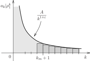
Figure 1: Illustration of the upper bounding of the sum of the terms $|a_{k}|\rho_{1}^{k}$ by an integral.

It is not a difficult task to establish the absolute and uniform convergence of a complex power series on a circle centered at the origin, or the lack thereof, starting from the behavior of the terms of the series in the limit $k\to\infty$, if we assume that they behave as inverse powers of $k$ for large values of $k$. If we have a complex power series $S_{z}$ with coefficients $a_{k}$, at a point $z_{1}$ strictly inside the unit disk,

$$S_{z}=\sum_{k=1}^{\infty}a_{k}z_{1}^{k},$$

where $|z_{1}|=\rho_{1}$ and $\rho_{1}<1$, then it is absolutely convergent if and only if the series $\overline{S}_{z}$ of the absolute values of the coefficients,

$$\overline{S}_{z} = \sum_{k=1}^{\infty}|a_{k}||z_{1}|^{k}$$

$$= \sum_{k=1}^{\infty}|a_{k}|\rho_{1}^{k},$$

converges. One can show that this sum will be finite if, for $k$ above a certain minimum value $k_{m}$, it holds that

$$|a_{k}|\rho_{1}^{k}\leq\frac{A}{k^{1+\varepsilon}},$$

for some positive real constant $A$ and some real constant $\varepsilon>0$. This is true because the sum of a finite set of initial terms is necessarily finite, and because in this case we may bound the remaining infinite sum from above by a convergent asymptotic integral,

$$\sum_{k=k_{m}+1}^{\infty}|a_{k}|\rho_{1}^{k} \leq \sum_{k=k_{m}+1}^{\infty}\frac{A}{k^{1+\varepsilon}}$$

$$< \int_{k_{m}}^{\infty}dk\,\frac{A}{k^{1+\varepsilon}}$$

$$= \frac{-A}{\varepsilon}\,\frac{1}{k^{\varepsilon}}\left.\rule{0.0pt}{12.91663pt}\right[_{\,k_{m}}^{\,\infty}$$

$$= \frac{A}{\varepsilon}\,\frac{1}{k_{m}^{\varepsilon}},$$

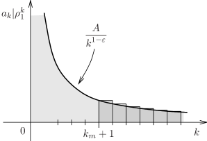
Figure 2: Illustration of the lower bounding of the sum of the terms $|a_{k}|\rho_{1}^{k}$ by an integral.

as illustrated in Figure 1. In that illustration each vertical rectangle has base $1$ and height given by $|a_{k}|\rho_{1}^{k}$, and therefore area given by $|a_{k}|\rho_{1}^{k}$. As one can see, the construction is such that the set of all such rectangles is below the graph of the function $A/k^{1+\varepsilon}$, and therefore the sum of their areas is contained within the area under that graph, to the right of $k_{m}$. This establishes the necessary inequality between the sum and the integral.

So long as $\varepsilon$ is not zero, this establishes an upper bound to a sum of positive quantities, which is therefore a monotonically increasing sum. It then follows from the well-known theorem of real analysis that the sum necessarily converges, and therefore the series $S_{z}$ is absolutely convergent at $z_{1}$.

In addition to this, one can see that the convergence condition does not depend on $\theta$, since that dependence is only within the complex variable $z=\rho_{1}\exp(\mbox{\boldmath$\imath$}\theta)$, and vanishes when we take absolute values. This implies uniform convergence because, given a strictly positive real number $\epsilon$, absolute convergence for this value of $\epsilon$ implies convergence for this same value of $\epsilon$, with the same solution $k(\epsilon)$ for the convergence condition. This makes it clear that the solution of the convergence condition for $k$ is independent of position and therefore that the series is also uniformly convergent on the circle of radius $\rho_{1}$ centered at the origin.

This establishes a sufficient condition for the absolute and uniform convergence of the complex power series on the circle. On the other hand, if we have that, for $k$ above a certain minimum value $k_{m}$,

$$|a_{k}|\rho_{1}^{k}\geq\frac{A}{k^{1-\varepsilon}},$$

with positive real $A$ and real $\varepsilon\geq 0$, then it is possible to bound the sum $\overline{S}_{v}$ from below by an asymptotic integral that diverges to positive infinity. This is done in a way similar to the one used for the establishment of the upper bound, but inverting the situation so as to keep the area under the graph contained within the combined areas of the rectangles, as illustrated in Figure 2. The argument then establishes in this case that, for $\varepsilon>0$

$$\sum_{k=k_{m}+1}^{\infty}|a_{k}|\rho_{1}^{k} \geq \sum_{k=k_{m}+1}^{\infty}\frac{A}{k^{1-\varepsilon}}$$

$$> \int_{k_{m}+1}^{\infty}dk\,\frac{A}{k^{1-\varepsilon}}$$

$$= \frac{A}{\varepsilon}\,k^{\varepsilon}\left.\rule{0.0pt}{12.91663pt}\right[_{\,k_{m}+1}^{\,\infty}$$

$$= -\,\frac{A}{\varepsilon}\,(k_{m}+1)^{\varepsilon}+\frac{A}{\varepsilon}\lim_{k\to\infty}k^{\varepsilon},$$

and therefore that $\overline{S}_{z}$ diverges to infinity. A similar calculation can be performed in the case $\varepsilon=0$, leading to logarithms and yielding the same conclusions. This does not prove or disprove convergence itself, but it does establish the absence of absolute convergence. It also shows that, so long as $|a_{k}|\rho_{1}^{k}$ behaves as a power of $k$ for large $k$, the previous condition is both sufficient and necessary for absolute convergence.

B.2 About the Ratio Test

Let us show that the Taylor series of an analytic function cannot satisfy the ratio test at the boundary of its maximum convergence disk. We will assume that the convergence disk is the open unit disk, but the proof can be easily generalized. It the series satisfies the test, then it follows that there is a strictly positive real number $q<1$ and an integer $k_{m}$ such that, for all $k>k_{m}$ we have

$$\frac{|a_{k+1}|}{|a_{k}|}\,|z|<q.$$

We observe now that since $|z|=1$ over the whole unit circle, this condition is in fact independent of the angular position and valid over the whole unit circle, so that we have

$$\frac{|a_{k+1}|}{|a_{k}|}<q.$$

Now, consider a point $z_{1}$ given by any value of $\theta$ and the value

$$|z_{1}|=\frac{q+1}{2q}$$

for the radius. Since $q$ is strictly positive and strictly smaller than one, we have that

$$q < 1\;\;\;\Rightarrow$$

$$q+q < q+1\;\;\;\Rightarrow$$

$$\frac{q+1}{2q} > 1.$$

It follows therefore that the point $z_{1}$ is strictly outside the unit disk. We consider now the ratio test for this new point. We start from the known valid condition on the unit disk, so that we have

$$\frac{|a_{k+1}|}{|a_{k}|} < q\;\;\;\Rightarrow$$

$$\frac{|a_{k+1}|}{|a_{k}|}\,|z_{1}| < \frac{q+1}{2}\;\;\;\Rightarrow$$

$$\frac{|a_{k+1}|}{|a_{k}|}\,|z_{1}| < q_{1},$$

which establishes the upper bound $q_{1}$. Besides, since we know that $q$ is strictly less than one, we also have that

$$q < 1\;\;\;\Rightarrow$$

$$q+1 < 1+1\;\;\;\Rightarrow$$

$$\frac{q+1}{2} < 1.$$

What we have concluded here is that $q_{1}<1$, and therefore we conclude that the series satisfies the ratio test at the new point, which is strictly outside the unit disk, and hence converges there. Therefore, the basic convergence theorem implies that the maximum disk of convergence of the series $S_{z}$ extends beyond the unit circle. This contradicts the hypothesis that the open unit disk is the maximum disk of convergence, and we conclude therefore that the series cannot satisfy the ratio test at the boundary of its maximum disk of convergence.

Another way to interpret this result is to say that, if the Taylor series $S_{z}$ does satisfy the ratio test at the boundary of a given disk, then that disk is not its maximum disk of convergence. It follows therefore that the maximum disk of convergence is larger than the given disk, and contains it.

Appendix C Appendix: Examples of Limits from Within

In this appendix we will give a few illustrative examples. We will explore the possibility of recovering values for the functions associated to either weakly convergent or flatly divergent Fourier series, using limits from the interior of the open unit disk. In some of these simple examples we will recover the original functions in closed form. As we will see, sometimes it is also possible to write the FC functions in closed form. At the same time, we will also explore the extension of the structure to singular objects such as the Dirac delta “function”.

C.1 A Regular Sine Series with All $k$

Consider the Fourier series of the one-cycle unit-amplitude sawtooth wave, which is just the linear function $\theta/\pi$ between $-\pi$ and $\pi$. As is well known it is given by the sine series

$$S_{\rm s}=-\,\frac{2}{\pi}\sum_{k=1}^{\infty}\frac{(-1)^{k}}{k}\,\sin(k\theta).$$

The corresponding FC series is then

$$\bar{S}_{\rm s}=-\,\frac{2}{\pi}\sum_{k=1}^{\infty}\frac{(-1)^{k}}{k}\,\cos(k\theta),$$

the complex $S_{v}$ series is given by

$$S_{v}=-\,\frac{2}{\pi}\sum_{k=1}^{\infty}\frac{(-1)^{k}}{k}\,v^{k},$$

and the complex power series $S_{z}$ is given by

$$S_{z}=-\,\frac{2}{\pi}\sum_{k=1}^{\infty}\frac{(-1)^{k}}{k}\,z^{k}.$$

The ratio test tells us that the disk of convergence of $S_{z}$ is the unit disk. If we consider the inner analytic function $w(z)$ within this disk we observe that $w(0)=0$, as expected. We have for the function and its derivative

$$w(z) = -\,\frac{2}{\pi}\sum_{k=1}^{\infty}\frac{(-1)^{k}}{k}\,z^{k}\;\;\;\Rightarrow$$

$$\frac{dw(z)}{dz} = -\,\frac{2}{\pi}\sum_{k=1}^{\infty}(-1)^{k}z^{k-1}$$

$$= -\,\frac{2}{\pi z}\sum_{k=1}^{\infty}(-z)^{k}.$$

This is a geometrical series and therefore we may write the derivative in closed form,

$$\frac{dw(z)}{dz} = -\,\frac{2}{\pi z}\,\frac{-z}{1+z}$$

$$= \frac{2}{\pi}\,\frac{1}{1+z}.$$

This function has a simple pole at the point where the one-cycle sawtooth wave is discontinuous. This is a hard singularity of degree $1$. It is now very simple to integrate in order to obtain the inner analytic function $w(z)$ in closed form, remembering that we should have $w(0)=0$,

$$w(z)=\frac{2}{\pi}\,\ln(1+z).$$

This function has a logarithmic singularity at the point where the one-cycle sawtooth wave is discontinuous. This is a borderline hard singularity. If we now rationalize the argument of the logarithm in order to write it in the form

$$1+z=R\,{\rm e}^{\mbox{\boldmath$\imath$}\alpha},$$

then the logarithm is given by

$$\ln\!\left(1+z\right)=\ln(R)+\mbox{\boldmath$\imath$}\alpha,$$

which allows us to identify the real and imaginary parts of $w(z)$. We may write for the argument

$$R\,{\rm e}^{\mbox{\boldmath$\imath$}\alpha} = 1+\rho\left[\cos(\theta)+\mbox{\boldmath$\imath$}\sin(\theta)\right]$$

$$= \left[1+\rho\cos(\theta)\right]+\mbox{\boldmath$\imath$}\left[\rho\sin(\theta)\right].$$

From this it follows, after some algebra, that we have

$$R(\rho,\theta) = \sqrt{1+2\rho\cos(\theta)+\rho^{2}},$$

$$\alpha(\rho,\theta) = \arctan\!\left[\frac{\rho\sin(\theta)}{1+\rho\cos(\theta)}\right].$$

The part which is of interest now is the imaginary one, which is related to the series $S_{\rm s}$,

$$\Im[w(z)]=\frac{2}{\pi}\,\arctan\!\left[\frac{\rho\sin(\theta)}{1+\rho\cos(\theta)}\right].$$

The $\rho\to 1$ limit of this quantity is the function $f_{\rm s}(\theta)$. If we consider the case $\theta=\pm\pi$, we immediately get zero, because the argument of the arc tangent is zero, and therefore we get $\alpha=0$. Therefore we have

$$f_{\rm s}(\pm\pi) = \lim_{\rho\to 1}\Im[w(\rho,\pm\pi)]$$

$$= 0.$$

This is the correct value for the Fourier-series representation of the one-cycle sawtooth wave at this point. For $\theta\neq\pm\pi$ we get

$$f_{\rm s}(\theta) = \lim_{\rho\to 1}\Im[w(z)]$$

$$= \frac{2}{\pi}\lim_{\rho\to 1}\arctan\!\left[\frac{\rho\sin(\theta)}{1+\rho\cos(\theta)}\right]$$

$$= \frac{2}{\pi}\arctan\!\left[\frac{\sin(\theta)}{1+\cos(\theta)}\right].$$

In order to solve this we write everything in terms of $\theta/2$, and thus obtain

$$f_{\rm s}(\theta) = \frac{2}{\pi}\arctan\!\left[\frac{2\sin(\theta/2)\cos(\theta/2)}{2\cos^{2}(\theta/2)}\right]$$

$$= \frac{2}{\pi}\arctan\!\left[\frac{\sin(\theta/2)}{\cos(\theta/2)}\right]$$

$$= \frac{2}{\pi}\arctan\!\left[\tan(\theta/2)\right]$$

$$= \frac{\theta}{\pi}.$$

This is the correct value for the one-cycle unit-amplitude sawtooth wave. The FC function is related to the real part

$$\Re[w(z)]=\frac{1}{\pi}\,\ln\!\left[1+2\rho\cos(\theta)+\rho^{2}\right].$$

In the $\rho\to 1$ limit this function is singular at $\theta=\pm\pi$. Away from this logarithmic singularity we may write

$$\bar{f}_{\rm s}(\theta) = \lim_{\rho\to 1}\Re[w(z)]$$

$$= \frac{1}{\pi}\,\ln\!\left[2+2\cos(\theta)\right]$$

$$= \frac{1}{\pi}\,\ln\!\left[4\cos^{2}(\theta/2)\right].$$

We see therefore that the FC function to the one-cycle sawtooth wave is a function with a logarithmic singularity at the point where the original function is discontinuous. The derivative of this conjugate function is easily calculated, and turns out to be

$$\frac{d\bar{f}_{\rm s}(\theta)}{d\theta}=\frac{1}{\pi}\,\frac{\cos(\theta)-1}{\sin(\theta)}.$$

This is a quite a simple function, with a simple pole at $\theta=\pm\pi$. Note that the logarithmic singularity of the FC function $\bar{f}_{\rm s}(\theta)$ is an integrable one, as one would expect since the Fourier coefficients are finite.

Note that we get a free set of integration formulas out of this effort. Since the coefficients $a_{k}$ can be written as integrals involving $\bar{f}_{\rm s}(\theta)$, we have at once that

$$\int_{-\pi}^{\pi}d\theta\,\ln\!\left[4\cos^{2}(\theta/2)\right]\cos(k\theta)=-\,\frac{2\pi(-1)^{k}}{k},$$

for $k>0$.

C.2 A Regular Sine Series with Odd $k$

Consider the Fourier series of the standard unit-amplitude square wave. As is well known it is given by the sine series

$$S_{\rm s}=\frac{4}{\pi}\sum_{j=0}^{\infty}\frac{1}{2j+1}\,\sin[(2j+1)\theta].$$

The corresponding FC series is then

$$\bar{S}_{\rm s}=\frac{4}{\pi}\sum_{j=0}^{\infty}\frac{1}{2j+1}\,\cos[(2j+1)\theta],$$

the complex $S_{v}$ series is given by

$$S_{v}=\frac{4}{\pi}\sum_{j=0}^{\infty}\frac{1}{2j+1}\,v^{2j+1},$$

and the complex power series $S_{z}$ is given by

$$S_{z}=\frac{4}{\pi}\sum_{j=0}^{\infty}\frac{1}{2j+1}\,z^{2j+1}.$$

The ratio test tells us that the disk of convergence of $S_{z}$ is the unit disk. If we consider the inner analytic function $w(z)$ within this disk we observe that $w(0)=0$, as expected. We have for the function and its derivative

$$w(z) = \frac{4}{\pi}\sum_{j=0}^{\infty}\frac{1}{2j+1}\,z^{2j+1}\;\;\;\Rightarrow$$

$$\frac{dw(z)}{dz} = \frac{4}{\pi}\sum_{j=0}^{\infty}z^{2j}.$$

This is a geometrical series and therefore we may write the derivative in closed form,

$$\frac{dw(z)}{dz} = \frac{4}{\pi}\,\frac{1}{1-z^{2}}$$

$$= \frac{2}{\pi}\,\left(\frac{1}{1+z}+\frac{1}{1-z}\right).$$

This function has two simple poles at the points where the square wave is discontinuous. These are hard singularities of degree $1$. It is now very simple to integrate in order to obtain the inner analytic function $w(z)$ in closed form, remembering that we should have $w(0)=0$,

$$w(z) = \frac{2}{\pi}\,\left[\ln(1+z)-\ln(1-z)\right]$$

$$= \frac{2}{\pi}\,\ln\!\left(\frac{1+z}{1-z}\right).$$

This function has logarithmic singularities at the points where the square wave is discontinuous. These are borderline hard singularities. If we now rationalize the argument of the logarithm in order to write it in the form

$$\frac{1+z}{1-z}=R\,{\rm e}^{\mbox{\boldmath$\imath$}\alpha},$$

then the logarithm is given by

$$\ln\!\left(\frac{1+z}{1-z}\right)=\ln(R)+\mbox{\boldmath$\imath$}\alpha,$$

which allows us to identify the real and imaginary parts of $w(z)$. We may write for the argument

$$R\,{\rm e}^{\mbox{\boldmath$\imath$}\alpha} = \frac{(1+z)(1-z*)}{(1-z)(1-z*)}$$

$$= \frac{1+2\mbox{\boldmath$\imath$}\rho\sin(\theta)-\rho^{2}}{1-2\rho\cos(\theta)+\rho^{2}}$$

$$= \frac{\left(1-\rho^{2}\right)}{\left(1+\rho^{2}\right)-2\rho\cos(\theta)}+\mbox{\boldmath$\imath$}\,\frac{2\rho\sin(\theta)}{\left(1+\rho^{2}\right)-2\rho\cos(\theta)}.$$

From this it follows, after some algebra, that we have

$$R(\rho,\theta) = \sqrt{\frac{\left(1+\rho^{2}\right)+2\rho\cos(\theta)}{\left(1+\rho^{2}\right)-2\rho\cos(\theta)}},$$

$$\alpha(\rho,\theta) = \arctan\!\left[\frac{2\rho\sin(\theta)}{1-\rho^{2}}\right].$$

The part which is of interest now is the imaginary one, which is related to the series $S_{\rm s}$,

$$\Im[w(z)]=\frac{2}{\pi}\,\arctan\!\left[\frac{2\rho\sin(\theta)}{1-\rho^{2}}\right].$$

The $\rho\to 1$ limit of this quantity is the function $f_{\rm s}(\theta)$. If we consider the cases $\theta=0$ and $\theta=\pm\pi$, we immediately get zero, because the argument of the arc tangent is zero, and therefore we get $\alpha=0$. Therefore we have

$$f_{\rm s}(0) = \lim_{\rho\to 1}\Im[w(\rho,0)]$$

$$= 0,$$

$$f_{\rm s}(\pm\pi) = \lim_{\rho\to 1}\Im[w(\rho,\pm\pi)]$$

$$= 0.$$

These are the correct values for the Fourier-series representation of the square wave at these points. For $\theta\neq 0$ and $\theta\neq\pm\pi$ we get

$$f_{\rm s}(\theta) = \lim_{\rho\to 1}\Im[w(z)]$$

$$= \frac{2}{\pi}\lim_{\rho\to 1}\arctan\!\left[\frac{2\rho\sin(\theta)}{1-\rho^{2}}\right]$$

$$= \frac{2}{\pi}\lim_{\rho\to 1}\arctan\!\left[\frac{2\sin(\theta)}{1-\rho^{2}}\right].$$

If $\theta>0$ the argument of the arc tangent goes to positive infinity in the limit, and therefore the arc tangent $\alpha$ approaches $\pi/2$. If $\theta>0$ the argument goes to negative infinity, and therefore $\alpha$ approaches $-\pi/2$. We get therefore the values

$$\begin{array}[]{rclcc}f_{\rm s}(\theta)&=&1&\mbox{for}&\theta>0,\\ f_{\rm s}(\theta)&=&-1&\mbox{for}&\theta<0,\end{array}$$

which completes the correct set of values for the standard square wave. The FC function is related to the real part

$$\Re[w(z)]=\frac{1}{\pi}\,\ln\!\left[\frac{\left(1+\rho^{2}\right)+2\rho\cos(\theta)}{\left(1+\rho^{2}\right)-2\rho\cos(\theta)}\right].$$

In the $\rho\to 1$ limit this function is singular at $\theta=0$ and $\theta=\pm\pi$. Away from these logarithmic singularities we may write

$$\bar{f}_{\rm s}(\theta) = \lim_{\rho\to 1}\Re[w(z)]$$

$$= \frac{1}{\pi}\,\ln\!\left[\frac{1+\cos(\theta)}{1-\cos(\theta)}\right].$$

We see therefore that the FC function to the square wave is a function with logarithmic singularities at the two points where the original function is discontinuous. The derivative of this conjugate function is easily calculated, and turns out to be

$$\frac{d\bar{f}_{\rm s}(\theta)}{d\theta}=-\,\frac{2}{\pi}\,\frac{1}{\sin(\theta)}.$$

This is a quite a simple function, with two simple poles at $\theta=0$ and $\theta=\pm\pi$. Note that the logarithmic singularities of the FC function $\bar{f}_{\rm s}(\theta)$ are integrable ones, as one would expect since the Fourier coefficients are finite.

Note that we get a free set of integration formulas out of this effort. Since the coefficients $a_{k}$ can be written as integrals involving $\bar{f}_{\rm s}(\theta)$, we have at once that for odd $k=2j+1$

$$\int_{-\pi}^{\pi}d\theta\,\ln\!\left[\frac{1+\cos(\theta)}{1-\cos(\theta)}\right]\cos(k\theta)=\frac{4\pi}{k},$$

while for even $k=2j$

$$\int_{-\pi}^{\pi}d\theta\,\ln\!\left[\frac{1+\cos(\theta)}{1-\cos(\theta)}\right]\cos(k\theta)=0,$$

for $k>0$. Note that $\bar{f}_{\rm s}(\theta)$ is an even function of $\theta$, so that these integrals are not zero by parity arguments, and therefore we also have

$$\int_{0}^{\pi}d\theta\,\ln\!\left[\frac{1+\cos(\theta)}{1-\cos(\theta)}\right]\cos(k\theta)=0,$$

for $k>0$.

C.3 A Regular Sine Series with Even $k$

Consider the Fourier series of the two-cycle unit-amplitude sawtooth wave. As is well known it is given by the sine series

$$S_{\rm s}=-\,\frac{4}{\pi}\sum_{j=1}^{\infty}\frac{1}{2j}\,\sin[(2j)\theta].$$

The corresponding FC series is then

$$\bar{S}_{\rm s}=-\,\frac{4}{\pi}\sum_{j=1}^{\infty}\frac{1}{2j}\,\cos[(2j)\theta],$$

the complex $S_{v}$ series is given by

$$S_{v}=-\,\frac{4}{\pi}\sum_{j=1}^{\infty}\frac{1}{2j}\,v^{2j},$$

and the complex power series $S_{z}$ is given by

$$S_{z}=-\,\frac{4}{\pi}\sum_{j=1}^{\infty}\frac{1}{2j}\,z^{2j}.$$

The ratio test tells us that the disk of convergence of $S_{z}$ is the unit disk. If we consider the inner analytic function $w(z)$ within this disk we observe that $w(0)=0$, as expected. We have for the function and its derivative

$$w(z) = -\,\frac{4}{\pi}\sum_{j=1}^{\infty}\frac{1}{2j}\,z^{2j}\;\;\;\Rightarrow$$

$$\frac{dw(z)}{dz} = -\,\frac{4}{\pi}\sum_{j=1}^{\infty}z^{2j-1}.$$

This is a geometrical series and therefore we may write the derivative in closed form,

$$\frac{dw(z)}{dz} = -\,\frac{4}{\pi}\,\frac{z}{1-z^{2}}$$

$$= \frac{2}{\pi}\,\left(\frac{1}{1+z}-\frac{1}{1-z}\right).$$

This function has two simple poles at the points where the two-cycle sawtooth wave is discontinuous. These are hard singularities of degree $1$. It is now very simple to integrate in order to obtain the inner analytic function $w(z)$ in closed form, remembering that we should have $w(0)=0$,

$$w(z) = \frac{2}{\pi}\,\left[\ln(1+z)+\ln(1-z)\right]$$

$$= \frac{2}{\pi}\,\ln\!\left(1-z^{2}\right).$$

This function has logarithmic singularities at the points where the two-cycle sawtooth wave is discontinuous. These are borderline hard singularities. If we now rationalize the argument of the logarithm in order to write it in the form

$$1-z^{2}=R\,{\rm e}^{\mbox{\boldmath$\imath$}\alpha},$$

then the logarithm is given by

$$\ln\!\left(1-z^{2}\right)=\ln(R)+\mbox{\boldmath$\imath$}\alpha,$$

which allows us to identify the real and imaginary parts of $w(z)$. We may write for the argument

$$R\,{\rm e}^{\mbox{\boldmath$\imath$}\alpha} = 1-\rho^{2}\left[\cos(2\theta)+\mbox{\boldmath$\imath$}\sin(2\theta)\right]$$

$$= \left[1-\rho^{2}\cos(2\theta)\right]-\mbox{\boldmath$\imath$}\left[\rho^{2}\sin(2\theta)\right].$$

From this it follows, after some algebra, that we have

$$R(\rho,\theta) = \sqrt{1-2\rho^{2}\cos(2\theta)+\rho^{4}},$$

$$\alpha(\rho,\theta) = -\arctan\!\left[\frac{\rho^{2}\sin(2\theta)}{1-\rho^{2}\cos(2\theta)}\right].$$

The part which is of interest now is the imaginary one, which is related to the series $S_{\rm s}$,

$$\Im[w(z)]=-\,\frac{2}{\pi}\,\arctan\!\left[\frac{\rho^{2}\sin(2\theta)}{1-\rho^{2}\cos(2\theta)}\right].$$

The $\rho\to 1$ limit of this quantity is the function $f_{\rm s}(\theta)$. If we consider the cases $\theta=0$ and $\theta=\pm\pi$, we immediately get zero, because the argument of the arc tangent is zero, and therefore we get $\alpha=0$. Therefore we have

$$f_{\rm s}(0) = \lim_{\rho\to 1}\Im[w(\rho,0)]$$

$$= 0,$$

$$f_{\rm s}(\pm\pi) = \lim_{\rho\to 1}\Im[w(\rho,\pm\pi)]$$

$$= 0.$$

These are the correct values for the Fourier-series representation of the two-cycle sawtooth wave at these points. For $\theta\neq 0$ and $\theta\neq\pm\pi$ we get

$$f_{\rm s}(\theta) = \lim_{\rho\to 1}\Im[w(z)]$$

$$= -\,\frac{2}{\pi}\lim_{\rho\to 1}\arctan\!\left[\frac{\rho^{2}\sin(2\theta)}{1-\rho^{2}\cos(2\theta)}\right]$$

$$= -\,\frac{2}{\pi}\arctan\!\left[\frac{\sin(2\theta)}{1-\cos(2\theta)}\right]$$

$$= -\,\frac{2}{\pi}\arctan\!\left[\frac{2\sin(\theta)\cos(\theta)}{2\sin^{2}(\theta)}\right]$$

$$= -\,\frac{2}{\pi}\arctan\!\left[\frac{\cos(\theta)}{\sin(\theta)}\right].$$

In order to solve this equation we first write it as

$$f_{\rm s}(\theta) = \frac{2}{\pi}\,\alpha(\theta),$$

$$\alpha(\theta) = -\,\arctan\!\left[\frac{\cos(\theta)}{\sin(\theta)}\right]\;\;\;\Rightarrow$$

$$\tan(\alpha) = -\,\frac{1}{\tan(\theta)}.$$

Keeping in mind that we must have $-\pi\leq\theta\leq\pi$ and $-\pi/2\leq\alpha\leq\pi/2$, and paying careful attention to the signs of the sine and cosine of either angle, one concludes that the solution is given by

$$\begin{array}[]{rclcc}\alpha(\theta)&=&\theta-{\displaystyle\frac{\displaystyle\pi}{\displaystyle 2}}&\mbox{for}&\theta>0,\\ \alpha(\theta)&=&\theta+{\displaystyle\frac{\displaystyle\pi}{\displaystyle 2}}&\mbox{for}&\theta<0,\end{array}$$

which means that for $f_{\rm s}(\theta)$ we have

$$\begin{array}[]{rclcc}f_{\rm s}(\theta)&=&{\displaystyle\frac{\displaystyle 2\theta}{\displaystyle\pi}}-1&\mbox{for}&\theta>0,\\ f_{\rm s}(\theta)&=&{\displaystyle\frac{\displaystyle 2\theta}{\displaystyle\pi}}+1&\mbox{for}&\theta<0.\end{array}$$

These are the correct values for the two-cycle unit-amplitude sawtooth wave. The FC function is related to the real part

$$\Re[w(z)]=\frac{1}{\pi}\,\ln\!\left[1-2\rho^{2}\cos(2\theta)+\rho^{4}\right].$$

In the $\rho\to 1$ limit this function is singular at $\theta=0$ and $\theta=\pm\pi$. Away from these logarithmic singularities we may write

$$\bar{f}_{\rm s}(\theta) = \lim_{\rho\to 1}\Re[w(z)]$$

$$= \frac{1}{\pi}\,\ln\!\left[2-2\cos(2\theta)\right]$$

$$= \frac{1}{\pi}\,\ln\!\left[4\sin^{2}(\theta)\right].$$

We see therefore that the FC function to the two-cycle sawtooth wave is a function with logarithmic singularities at the two points where the original function is discontinuous. The derivative of this conjugate function is easily calculated, and turns out to be

$$\frac{d\bar{f}_{\rm s}(\theta)}{d\theta}=\frac{2}{\pi}\,\frac{\cos(\theta)}{\sin(\theta)}.$$

This is a quite a simple function, with two simple poles at $\theta=0$ and $\theta=\pm\pi$. Note that the logarithmic singularities of the FC function $\bar{f}_{\rm s}(\theta)$ are integrable ones, as one would expect since the Fourier coefficients are finite.

Note that we get a free set of integration formulas out of this effort. Since the coefficients $a_{k}$ can be written as integrals involving $\bar{f}_{\rm s}(\theta)$, we have at once that for even $k=2j$

$$\int_{-\pi}^{\pi}d\theta\,\ln\!\left[4\sin^{2}(\theta)\right]\cos(k\theta)=-\,\frac{4\pi}{k},$$

for $k>0$, while for odd $k=2j+1$

$$\int_{-\pi}^{\pi}d\theta\,\ln\!\left[4\sin^{2}(\theta)\right]\cos(k\theta)=0.$$

Note that $\bar{f}_{\rm s}(\theta)$ is an even function of $\theta$, so that these integrals are not zero by parity arguments, and therefore we also have

$$\int_{0}^{\pi}d\theta\,\ln\!\left[4\sin^{2}(\theta)\right]\cos(k\theta)=0,$$

for $k=2j+1$.

C.4 A Regular Cosine Series with Odd $k$

Consider the Fourier series of the unit-amplitude triangular wave. As is well known it is given by the cosine series

$$S_{\rm c}=-\,\frac{8}{\pi^{2}}\sum_{j=0}^{\infty}\frac{1}{(2j+1)^{2}}\,\cos[(2j+1)\theta].$$

The corresponding FC series is then

$$\bar{S}_{\rm c}=-\,\frac{8}{\pi^{2}}\sum_{j=0}^{\infty}\frac{1}{(2j+1)^{2}}\,\sin[(2j+1)\theta],$$

the complex $S_{v}$ series is given by

$$S_{v}=-\,\frac{8}{\pi^{2}}\sum_{j=0}^{\infty}\frac{1}{(2j+1)^{2}}\,v^{2j+1},$$

and the complex power series $S_{z}$ is given by

$$S_{z}=-\,\frac{8}{\pi^{2}}\sum_{j=0}^{\infty}\frac{1}{(2j+1)^{2}}\,z^{2j+1}.$$

The ratio test tells us that the disk of convergence of $S_{z}$ is the unit disk. If we consider the inner analytic function $w(z)$ within this disk we observe that $w(0)=0$, as expected. We have for the function and its derivative

$$w(z) = -\,\frac{8}{\pi^{2}}\sum_{j=0}^{\infty}\frac{1}{(2j+1)^{2}}\,z^{2j+1}\;\;\;\Rightarrow$$

$$\frac{dw(z)}{dz} = -\,\frac{8}{\pi^{2}}\sum_{j=0}^{\infty}\frac{1}{2j+1}\,z^{2j}.$$

Observe that we have for the derivative the particular value

$$\frac{dw}{dz}(0)=-\,\frac{8}{\pi^{2}}.$$

We may now multiply by $z$ and differentiate again, to obtain

$$\frac{d}{dz}\left[z\,\frac{dw(z)}{dz}\right] = -\,\frac{8}{\pi^{2}}\,\frac{d}{dz}\sum_{j=0}^{\infty}\frac{1}{2j+1}\,z^{2j+1}$$

$$= -\,\frac{8}{\pi^{2}}\sum_{j=0}^{\infty}z^{2j}.$$

This is a geometrical series and therefore we may write this expression in closed form,

$$\frac{d}{dz}\left[z\,\frac{dw(z)}{dz}\right] = -\,\frac{8}{\pi^{2}}\,\frac{1}{1-z^{2}}$$

$$= -\,\frac{8}{\pi^{2}}\,\left(\frac{1}{1+z}+\frac{1}{1-z}\right).$$

It is now very simple to integrate in order to obtain the derivative of $w(z)$ in closed form, remembering that we should have for it the value $-8/\pi^{2}$ at $z=0$,

$$z\,\frac{dw(z)}{dz} = -\,\frac{4}{\pi^{2}}\,\left[\ln(1+z)-\ln(1-z)\right]$$

$$= -\,\frac{4}{\pi^{2}}\,\ln\!\left(\frac{1+z}{1-z}\right).$$

This is the logarithmic derivative of $w(z)$, which is another inner analytic function, and it should be noted that it is proportional to the analytic function $w_{\rm sq}(z)$ for the case of the standard square wave,

$$z\,\frac{dw(z)}{dz}=-\,\frac{2}{\pi}\,w_{\rm sq}(z).$$

We get for the derivative of $w(z)$

$$\frac{dw(z)}{dz}=-\,\frac{4}{\pi^{2}}\,\frac{1}{z}\,\ln\!\left(\frac{1+z}{1-z}\right).$$

This function has two borderline hard singularities at the points where the triangular wave is not differentiable. Presumably $w(z)$ has two borderline soft singularities at these points. It seems that the second integration cannot be done explicitly because the indefinite integral of the function above cannot be expressed as a finite combination of elementary functions. We are thus unable to write $w(z)$ in closed form. However, we may still obtain partial confirmation of our results by using the closed form for the derivative of $w(z)$. If we differentiate the Fourier series of the triangular wave with respect to $\theta$ we get

$$\frac{dS_{\rm c}}{d\theta}=\frac{8}{\pi^{2}}\sum_{j=0}^{\infty}\frac{1}{2j+1}\,\sin[(2j+1)\theta].$$

This is equal to $2/\pi$ times the Fourier series for the standard square wave, given in Subsection C.2. On the other hand, if we use $z=\rho\exp(\mbox{\boldmath$\imath$}\theta)$ and consider the complex derivative of $w(z)$ taken in the direction of $\theta$, we have

$$\frac{dw(z)}{d\theta}=\mbox{\boldmath$\imath$}z\,\frac{dw(z)}{dz}.$$

We have therefore

$$\frac{dw(z)}{d\theta} = -\mbox{\boldmath$\imath$}\,\frac{4}{\pi^{2}}\,\ln\!\left(\frac{1+z}{1-z}\right)$$

$$= -\mbox{\boldmath$\imath$}\,\frac{2}{\pi}\,w_{\rm sq}(z).$$

The factor of $-\mbox{\boldmath$\imath$}$ simply implements the necessary exchanges of real and imaginary parts, to account for the exchange of sines and cosines in the process of differentiation, and the factor of $2/\pi$ corrects the normalization. We see therefore that at least the derivative of the Fourier series at the unit circle is represented correctly by the inner analytic function $w(z)$.

C.5 A Singular Cosine Series

Consider the Fourier series of the Dirac delta “function” centered at $\theta=\theta_{1}$, which we denote by $\delta(\theta-\theta_{1})$. We may easily calculate its Fourier coefficients using the rules of manipulation of $\delta(\theta-\theta_{1})$, thus obtaining $\alpha_{k}=\cos(k\theta_{1})/\pi$ and $\beta_{k}=\sin(k\theta_{1})/\pi$ for all $k$. The series is therefore the complete Fourier series given by

$$S_{\rm c} = \frac{1}{2\pi}+\frac{1}{\pi}\sum_{k=1}^{\infty}\left[\cos(k\theta_{1})\cos(k\theta)+\sin(k\theta_{1})\sin(k\theta)\right]$$

$$= \frac{1}{2\pi}+\frac{1}{\pi}\sum_{k=1}^{\infty}\cos(k\Delta\theta),$$

where $\Delta\theta=\theta-\theta_{1}$. Apart from the constant term this is in fact a cosine series on this new variable. Clearly, this series diverges at all points in the interval $[-\pi,\pi]$. Undaunted by this, we construct the FC series, with respect to the new variable $\Delta\theta$,

$$\bar{S}_{\rm c}=\frac{1}{\pi}\sum_{k=1}^{\infty}\sin(k\Delta\theta),$$

a series that is also divergent, this time almost everywhere. If we define $v=\exp(\mbox{\boldmath$\imath$}\theta)$ and $v_{1}=\exp(\mbox{\boldmath$\imath$}\theta_{1})$ the corresponding complex series $S_{v}$ is then given by

$$S_{v}=\frac{1}{2\pi}+\frac{1}{\pi}\sum_{k=1}^{\infty}\left(\frac{v}{v_{1}}\right)^{k},$$

where we included the $k=0$ term, and the corresponding complex power series $S_{z}$ is given by

$$S_{z}=\frac{1}{2\pi}+\frac{1}{\pi}\sum_{k=1}^{\infty}\left(\frac{z}{z_{1}}\right)^{k},$$

where $z=\rho v$ and $z_{1}=v_{1}$ is a point on the unit circle. This is a geometrical series that converges everywhere strictly inside the unit disk, where it therefore converges to the analytic function

$$w_{\delta}(z)=\frac{1}{2\pi}-\frac{1}{\pi}\,\frac{z}{z-z_{1}}.$$

This function has a simple pole at the singular point of the Dirac delta “function”. This is a hard singularity of degree $1$. As was discussed in Section 6, strictly speaking this is not an inner analytic function by the definition which we adopted here, for two reasons. First, $w_{\delta}(0)$ is not zero, which is easily fixed by just taking off the constant term. Second, it does not reduce to a real function over the real axis. However, as was shown in Section 6, it does reduce to a real function over the straight line $z=\chi z_{1}$, with real $\chi$, since in this case we have

$$w(z)=-\,\frac{1}{\pi}\,\frac{\chi}{\chi-1},$$

which is a real function of the real variable $\chi$. Since we have $z_{1}=\exp(\mbox{\boldmath$\imath$}\theta_{1})$, we see that this is an inner analytic function rotated by an angle $\theta_{1}$ around the origin. We see therefore that our definition of inner analytic function can be easily generalized in this way, to make reference to any straight line going through the origin. We also see that there is nothing to prevent us from treating this function just like any other inner analytic function.

We now examine the real part of the function $w_{\delta}(z)$, which was derived in Section 6, and which is related to the series $S_{\rm c}$,

$$\Re[w_{\delta}(z)]=\frac{1}{2\pi}-\frac{1}{\pi}\,\frac{\rho\left[\rho-\cos(\Delta\theta)\right]}{\left(\rho^{2}+1\right)-2\rho\cos(\Delta\theta)}.$$

The $\rho\to 1$ limit of $\Re[w_{\delta}(z)]$ gives us back the constant term and the original cosine series $S_{\rm c}$, and in fact attributes well-defined finite values to it almost everywhere, even though the original series is divergent. As was shown directly in Section 6, in the $\rho\to 1$ limit this real part has all the required properties of the Dirac delta “function”, including the fact that it assumes the value zero almost everywhere. Note that although the singularity of $w_{\delta}(z)$ at $z=z_{1}$ is a simple pole and thus not an integrable one, the real part of $w_{\delta}(z)$ is integrable if one crosses the singularity in a specific direction, which in this case is the direction of the integration along the unit circle.

It is interesting that we may also write a closed expression for the real function which is the FC function of the Dirac delta “function”. We just consider the imaginary part of $w_{\delta}(z)$, which is related to the series $\bar{S}_{\rm c}$,

$$\Im[w_{\delta}(z)]=\frac{1}{\pi}\,\frac{\rho\sin(\Delta\theta)}{\left(\rho^{2}+1\right)-2\rho\cos(\Delta\theta)}.$$

We now take the $\rho\to 1$ limit, assuming that $\Delta\theta\neq 0$, and since this is an actual function we may write

$$\bar{f}_{\rm c}(\Delta\theta) = \lim_{\rho\to 1}\Im[w_{\delta}(z)]$$

$$= \frac{1}{2\pi}\,\frac{\sin(\Delta\theta)}{1-\cos(\Delta\theta)}$$

$$= \frac{1}{2\pi}\,\frac{1+\cos(\Delta\theta)}{\sin(\Delta\theta)}.$$

This is just a regular function except for a simple pole at $\Delta\theta=0$, and in fact quite a simple rational function involving trigonometric functions.

Note that we get a free set of integration formulas out of this effort. Since the coefficients $a_{k}$ can be written as integrals involving $\bar{f}_{\rm c}(\Delta\theta)$, we have at once that for all $k>0$

$$\int_{-\pi}^{\pi}d\theta\,\frac{1+\cos(\Delta\theta)}{\sin(\Delta\theta)}\,\sin(k\Delta\theta)=2\pi.$$

We may easily construct from this single Dirac delta “function” a pair of such “functions” which relates to the derivative of the standard square wave. All we have to do is to use the values $\theta_{1}=0$ and $\theta_{1}=\pi$ and add to the delta “function” at zero given by $2\delta(\theta-0)$ the delta “function” at $\pi$ given by $-2\delta(\theta-\pi)$. If we call the corresponding analytic functions $w_{0}(z)$ and $w_{\pi}(z)$, we have for the function $w_{2\delta}(z)$ corresponding to the pair

$$w_{0}(z) = \frac{1}{\pi}+\frac{2}{\pi}\,\frac{z}{1-z}\;\;\;\Rightarrow$$

$$w_{\pi}(z) = -\,\frac{1}{\pi}+\frac{2}{\pi}\,\frac{z}{1+z}\;\;\;\Rightarrow$$

$$w_{2\delta}(z) = \frac{2}{\pi}\,\frac{z}{1-z}+\frac{2}{\pi}\,\frac{z}{1+z}$$

$$= \frac{4}{\pi}\,\frac{z}{1-z^{2}}.$$

This is an inner analytic function with two simple poles, one at $z=1$ and one at $z=-1$. If, on the other hand, we consider the logarithmic derivative of the analytic function $w_{\rm sq}(z)$ of the standard square wave, we get

$$z\,\frac{dw_{\rm sq}(z)}{dz} = \frac{2}{\pi}\,z\,\frac{d}{dz}\ln\!\left(\frac{1+z}{1-z}\right)$$

$$= \frac{2}{\pi}\,z\,\left(\frac{1}{1+z}+\frac{1}{1-z}\right)$$

$$= \frac{4}{\pi}\,\frac{z}{1-z^{2}}.$$

We see therefore that we do indeed have

$$w_{2\delta}(z)=z\,\frac{dw_{\rm sq}(z)}{dz}.$$

In terms of derivatives with respect to $\theta$ this is written as

$$w_{2\delta}(z)=-\mbox{\boldmath$\imath$}\,\frac{dw_{\rm sq}(z)}{d\theta},$$

where once again the factor of $-\mbox{\boldmath$\imath$}$ has the role of exchanging real and imaginary parts, and thus sines and cosines.

Observe that this is an example in which, although the function $w_{\delta}(z)$ is analytic on the open unit disk, the series $S_{z}$ is not convergent on any points of the unit circle, and hence the two FC Fourier series do not converge together on any points of the unit circle. It is therefore outside the hypotheses we used in most of this paper, but it is still full of meaning. This indicates that there is more in this structure than has been analyzed so far. If fact, it is quite possible that the whole structure of distributions such as the one related to the Dirac delta “function” is lurking on the rim of the maximum disk of convergence of the series $S_{z}$ of the inner analytic functions $w_{\delta}(z)$ corresponding to divergent trigonometric series, that is, on the rim of the unit disk.

References

- [1] J. L. deLyra, “Fourier Theory on the Complex Plane II – Weak Convergence, Classification and Factorization of Singularities”, arXiv: 1409.4435.
- [2] See, for example, R. V. Churchill and J. W. Brown, “Complex Variables and Applications”, McGraw-Hill Book Co., 1995, and the references therein.
- [3] See, for example, R. V. Churchill and J. W. Brown, “Fourier Series and Boundary Value Problems”, McGraw-Hill Book Co., 2011, and the references therein.
-
[4]
See, for example, the URL
http://en.wikipedia.org/wiki/Harmonic_conjugate
and the references therein. -
[5]
See, for example, the URL
http://en.wikipedia.org/wiki/Hilbert_transform
and the references therein. -
[6]
See, for example, the URL
http://en.wikipedia.org/wiki/Abel’s_theorem
and the references therein. - [7] Joseph Gerver, “The Differentiability of the Riemann Function at Certain Rational Multiples of ”, Proc Natl Acad Sci USA, Mar 1969; 62(3): 668—670, and references therein.
-
[8]
See, for example, the URL
http://en.wikipedia.org/wiki/Lacunary_function
and the references therein. -
[9]
See, for example, the URLs
http://en.wikipedia.org/wiki/Fabry_gap_theorem
and the references therein.
http://en.wikipedia.org/wiki/Ostrowski-Hadamard_gap_theorem