Feedback Control of Switched Stochastic Systems Using
Randomly Available Active Mode Information

Abstract

Almost sure asymptotic stabilization of a discrete-time switched stochastic system is investigated. Information on the active operation mode of the switched system is assumed to be available for control purposes only at random time instants. We propose a stabilizing feedback control framework that utilizes the information obtained through mode observations. We first consider the case where stochastic properties of mode observation instants are fully known. We obtain sufficient asymptotic stabilization conditions for the closed-loop switched stochastic system under our proposed control law. We then explore the case where exact knowledge of the stochastic properties of mode observation instants is not available. We present a set of alternative stabilization conditions for this case. The results for both cases are predicated on the analysis of a sequence-valued process that encapsulates the stochastic nature of the evolution of active operation mode between mode observation instants. Finally, we demonstrate the efficacy of our results with numerical examples.

,

1 Introduction

The framework developed for switched stochastic systems provides accurate characterization of numerous complex real life processes from physics and engineering fields that are subject to randomly occurring incidents such as sudden environmental variations or sharp dynamical changes (?; ?). Stabilization problem for switched stochastic systems has been investigated in many studies (e.g., ?, ?, ?, ?, ?, ? and the references therein).

Control frameworks developed for switched stochastic systems often require the availability of information on the active operation mode at all times. Note that for numerous applications the active mode describes the operating conditions of a physical process and is driven by external incidents of stochastic nature. The active mode, hence, may not be directly measurable and it may not be available for control purposes at all time instants during the course of operation. When the controller does not have access to any mode information, for achieving stabilization one can resort to adaptive control frameworks (?; ?; ?) or mode-independent control laws (?; ?). On the other hand, if mode information can be observed at certain time instants (even if rarely), this information can be utilized in the control framework. In our earlier work (?; ?), we investigated stabilization of switched stochastic systems for the case where only sampled mode information is available for control purposes. Under the assumption that the active mode is periodically observed, we proposed a stabilizing feedback control framework that utilizes the available mode information.

In practical applications, it would be ideal if the mode information of a switched system is available for control purposes at all time instants or at least periodically. However, there are cases where mode information is obtained at random time instants. This situation occurs for example when the mode is sampled at all time instants; however, some of the mode samples are randomly lost during communication between mode sampling mechanism and the controller. On the other hand, in some applications, the mode has to be detected, but the detected mode information may not always be accurate. In this case each mode detection has a confidence level. Mode information with low confidence is discarded. As a result, depending on the confidence level of detection, the controller may or may not receive the mode information at a particular mode detection instant. In addition, we may also take advantage of random sampling for certain cases and observe the mode intentionally at random instants, as for such cases control under random sampling provides better results compared to periodic sampling. Note that random sampling has also been used for problems such as signal reconstruction and has been shown to have advantages over regular periodic sampling (see ?, ?).

In this paper our goal is to explore the feedback stabilization problem for the case where the active operation mode, which is modeled as a finite-state Markov chain, is observed at random time instants. We provide an extended discussion based on our preliminary report (?). Specifically, we assume that the length of intervals between consecutive mode observation instants are identically distributed independent random variables. We employ a renewal process to characterize the occurrences of random mode observations. This characterization allows us to also explore periodic mode observations (?; ?) as a special case.

We propose a linear feedback control law with a piecewise-constant gain matrix that is switched depending on the value of a randomly sampled version of the mode signal. In order to investigate the evolution of the active mode together with its randomly sampled version, we construct a stochastic process that represents sequences of values the mode takes between random mode observation instants. This sequence-valued stochastic process turns out to be a countable-state Markov chain defined over a set that is composed of all possible mode sequences of finite length. We first analyze the probabilistic dynamics of this sequence-valued Markov chain. Then based on our analysis, we obtain sufficient stabilization conditions for the closed-loop switched stochastic system under our proposed control framework. These stabilization conditions let us assess whether the closed-loop system is stable for a given probability distribution for the length of intervals between consecutive mode observation instants. As this probability distribution is not assumed to have a certain structure, the result presented in this paper can also be considered as a generalization of the result provided in ?, where stabilization problem is discussed in continuous time and the random intervals between mode sampling instants are specifically assumed to be exponentially distributed. In this paper we also explore the case where perfect information regarding the probability distribution for the length of intervals between consecutive mode observation instants is not available. For this problem setting, we present alternative sufficient stabilization conditions which can be used for verifying stability even if the distribution is not exactly known.

The paper is organized as follows. We provide the notation and a review of key results concerning renewal processes in Section 2. In Section 3, we propose our feedback control framework for stabilizing discrete-time switched stochastic systems under randomly available mode information. Then in Section 4, we present sufficient conditions under which our proposed control law guarantees almost sure asymptotic stabilization. In Section 5, we demonstrate the efficacy of our results with two illustrative numerical examples. Finally, in Section 6 we conclude our paper.

2 Mathematical Preliminaries

In this section, we provide notation and several definitions concerning discrete-time stochastic processes. Specifically, we denote positive and nonnegative integers by $\mathbb{N}$ and $\mathbb{N}_{0}$, respectively. Moreover, $\mathbb{R}$ denotes the set of real numbers, $\mathbb{R}^{n}$ denotes the set of $n\times 1$ real column vectors, and $\mathbb{R}^{n\times m}$ denotes the set of $n\times m$ real matrices. We write $(\cdot)^{\mathrm{T}}$ for transpose, $\|\cdot\|$ for the Euclidean vector norm. We use $\lambda_{\min}(H)$ (resp., $\lambda_{\max}(H)$) for the minimum (resp., maximum) eigenvalue of the Hermitian matrix $H$. A function $V:\mathbb{R}^{n}\rightarrow\mathbb{R}$ is called positive definite if $V(x)>0,\,x\neq 0$, and $V(0)=0$. We represent a finite-length sequence of ordered elements $q_{1},q_{2},\ldots,q_{n}$ by $q=(q_{1},q_{2},\ldots,q_{n})$. The length (number of elements) of the sequence $q$ is denoted by $|q|$. The notations $\mathrm{\mathbb{P}}[\cdot]$ and $\mathbb{E}[\cdot]$ respectively denote the probability and expectation on a probability space $(\Omega,\mathcal{F},\mathbb{P})$ with filtration $\{\mathcal{F}_{k}\}_{k\in\mathbb{N}_{0}}$. Furthermore, we write $\mathds{1}_{[G]}:\Omega\to\{0,1\}$ for the indicator of the set $G\in\mathcal{F}$, that is, $\mathds{1}_{[G]}(\omega)=1$, $\omega\in G$, and $\mathds{1}_{[G]}(\omega)=0$, $\omega\notin G$.

2.1 Discrete-Time Renewal Processes

A discrete-time renewal process $\{N(k)\in\mathbb{N}_{0}\}_{k\in\mathbb{N}_{0}}$ with initial value $N(0)=0$ is an $\mathcal{F}_{k}$-adapted stochastic counting process defined by $N(k)\triangleq\sum_{i\in\mathbb{N}}\mathds{1}_{[t_{i}\leq k]},$ where $t_{i}\in\mathbb{N}_{0}$, $i\in\mathbb{N}_{0}$, are random time instants such that $t_{0}=0$ and $\tau_{i}\triangleq t_{i}-t_{i-1}\in\mathbb{N}$, $i\in\mathbb{N}$, are identically distributed independent random variables with finite expectation (i.e., $\mathbb{E}[\tau_{i}]<\infty$, $i\in\mathbb{N}$). Note that $\tau_{i}$, $i\in\mathbb{N}$, denote the lengths of intervals between time instants $t_{i}$, $i\in\mathbb{N}_{0}$. Furthermore, we use $\mu:\mathbb{N}\to[0,1]$ to denote the common distribution of the random variables $\tau_{i}$, $i\in\mathbb{N}$, such that

$$\mathbb{P}[\tau_{i}=\tau] =\mu_{\tau},\quad\tau\in\mathbb{N},\quad i\in\mathbb{N},$$ (1)

where $\mu_{\tau}\in[0,1]$. Note that $\sum_{\tau\in\mathbb{N}}\mu_{\tau}=1$. Now, let $\hat{\tau}\triangleq\sum_{\tau\in\mathbb{N}}\tau\mu_{\tau}=\mathbb{E}[\tau_{1}]$($=\mathbb{E}[\tau_{i}]$, $i\in\mathbb{N}$). It follows as a consequence of strong law of large numbers for renewal processes (see ?) that $\lim_{k\to\infty}\frac{N(k)}{k}=\frac{1}{\hat{\tau}}$.

Note that in Section 3, we employ a renewal process to characterize the occurrences of random mode observations.

2.2 Almost Sure Asymptotic Stability

The zero solution $x(k)\equiv 0$ of a stochastic system is almost surely stable if, for all $\epsilon>0$ and $\rho>0$, there exists $\delta=\delta(\epsilon,\rho)>0$ such that if $\|x(0)\|<\delta$, then

$$\mathbb{P}[\sup_{k\in\mathbb{N}_{0}}\|x(k)\|>\epsilon] <\rho.$$ (2)

Furthermore, the zero solution $x(k)\equiv 0$ of a stochastic system is asymptotically stable almost surely if it is almost surely stable and

$$\mathbb{P}[\lim_{k\to\infty}\|x(k)\|=0] =1.$$ (3)

In Sections 3 and 4, we investigate almost sure asymptotic stabilization of a switched stochastic system.

3 Stabilizing Switched Stochastic Systems with Randomly Available Mode Information

In this section, we propose a feedback control framework for stabilizing a switched stochastic system by using only the randomly available mode information. Specifically, we consider the discrete-time switched linear stochastic system with $M\in\mathbb{N}$ number of modes given by

$$x(k+1)=A_{r(k)}x(k)+B_{r(k)}u(k),\quad k\in\mathbb{N}_{0},$$ (4)

with the initial conditions $x(0)=x_{0}$, $r(0)=r_{0}\in\mathcal{M}\triangleq\{1,2,\ldots,M\}$, where $x(k)\in\mathbb{R}^{n}$ and $u(k)\in\mathbb{R}^{m}$ respectively denote the state vector and the control input; furthermore, $A_{i}\in\mathbb{R}^{n\times n},\,B_{i}\in\mathbb{R}^{n\times m},\,i\in\mathcal{M}$, are the subsystem matrices. The mode signal $\{r(k)\in\mathcal{M}\}_{k\in\mathbb{N}_{0}}$ is assumed to be an $\mathcal{F}_{k}$-adapted, $M$-state discrete-time Markov chain with the initial distribution denoted by $\nu:\mathcal{M}\to[0,1]$ such that $\nu_{r_{0}}=1$ and $\nu_{i}=0$, $i\neq r_{0}$.

We use the matrix $P\in\mathbb{R}^{M\times M}$ to characterize probability of transitions between the modes of the switched system. Specifically, $p_{i,j}\in[0,1]$, which is the $(i,j)$th entry of the matrix $P$, denotes the probability of a transition from mode $i$ to mode $j$. Note that $\sum_{j\in\mathcal{M}}p_{i,j}=1$, $i\in\mathcal{M}$. Furthermore, we use $p_{i,j}^{(l)}$ to denote $(i,j)$th entry of the matrix $P^{l}$. Note that $p_{i,j}^{(l)}\in[0,1]$ is in fact the $l$-step transition probability from mode $i$ to mode $j$, that is,

$$p_{i,j}^{(l)} \triangleq\mathbb{P}[r(k+l)=j|r(k)=i],\,\,l\in\mathbb{N}_{0},\,\,i,j\in\mathcal{M},$$ (5)

with $p_{i,i}^{(0)}=1$, $i\in\mathcal{M}$, $p_{i,j}^{(0)}=0$, $i\neq j$. Furthermore, $p_{i,j}^{(1)}=p_{i,j}$, $i,j\in\mathcal{M}$. The mode signal can be represented using a transition diagram, which shows possible transitions between the operation modes of the switched system. Mode transition diagram for a switched system with two modes is shown in Figure 1.

In this paper, we assume that the mode signal is an aperiodic, irreducible Markov chain and has the invariant distribution $\pi:\mathcal{M}\to[0,1]$.

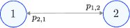
Figure 1: Mode transition diagram for $\{r(k)\in\mathcal{M}\triangleq\{1,2\}\}_{k\in\mathbb{N}_{0}}$

3.1 Feedback Control Under Randomly Observed Mode Information

In this paper, active mode of the switched stochastic system (4) is assumed to be observed only at random time instants, which we denote by $t_{i}\in\mathbb{N}_{0}$, $i\in\mathbb{N}_{0}$. We assume that $t_{0}=0$ and $\tau_{i}\triangleq t_{i}-t_{i-1}\in\mathbb{N}$, $i\in\mathbb{N}$, are independent random variables that are distributed according to a common distribution $\mu:\mathbb{N}\to[0,1]$ for all $i\in\mathbb{N}$ such that $\hat{\tau}\triangleq\sum_{\tau\in\mathbb{N}}\tau\mu_{\tau}<\infty$. In this problem setting, the initial mode information $r_{0}$ is assumed to be available to the controller, and a renewal process $\{N(k)\in\mathbb{N}_{0}\}_{k\in\mathbb{N}_{0}}$ is employed for counting the number of mode observations that are obtained after the initial time. We assume that the renewal process $\{N(k)\in\mathbb{N}_{0}\}_{k\in\mathbb{N}_{0}}$ and the mode signal $\{r(k)\in\mathcal{M}\}_{k\in\mathbb{N}_{0}}$ are mutually independent.

Following our approach in ?, ?, ?, we employ a linear feedback control law with a ‘piecewise-constant’ feedback gain matrix that depends only on the obtained mode information. Specifically, we consider the control law

$$u(k) =K_{\sigma(k)}x(k),\quad k\in\mathbb{N}_{0},$$ (6)

where $\{\sigma(k)\in\mathcal{M}\}_{k\in\mathbb{N}_{0}}$ is the sampled version of the mode signal defined by

$$\sigma(k) \triangleq r(t_{N(k)}),\quad k\in\mathbb{N}_{0}.$$ (7)

Note that the sampled mode signal $\{\sigma(k)\in\mathcal{M}\}_{k\in\mathbb{N}_{0}}$ acts as a switching mechanism for the linear feedback gain, which remains constant between two consecutive mode observation instants, that is, $K_{\sigma(k)}=K_{r(t_{i})}$ for $k\in[t_{i},t_{i+1})$.

Between two consecutive mode observation instants, the feedback gain $K_{\sigma(\cdot)}$ stays constant, whereas the active mode $r(\cdot)$ of the dynamical system (4) may change its value. Stabilization performance under the control law (6) hence depends not only on the length of the intervals between random mode observation instants, but also on how the active mode switches during the intervals.

In Figure 2, we show sample paths of the active mode signal $r(\cdot)$ and its sampled version $\sigma(\cdot)$ for a switched stochastic system with $M=2$ modes. In this example, active mode is observed at time instants $t_{0}=0$, $t_{1}=2$, $t_{2}=5$, $t_{3}=6$, $t_{4}=8$, $\ldots$. Note that at mode observation instants actual mode signal $r(\cdot)$ and its sampled version $\sigma(\cdot)$ have the same value. However, at the other time instants, sampled mode signal may differ from the actual mode, since between mode observation instants, system mode may switch.

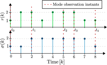
Figure 2: Actual mode $r(k)$ and its sampled version $\sigma(k)$

In order to investigate the evolution of the active mode between consecutive mode observation instants, we construct a new stochastic process $\{s(i)\}_{i\in\mathbb{N}_{0}}$ that takes values from a countable set of mode sequences of variable length. Specifically, we define $\{s(i)\}_{i\in\mathbb{N}_{0}}$ by

$$s(i) \triangleq\big{(}r(t_{i}),r(t_{i}+1),\ldots,r(t_{i+1}-1)\big{)},\,\,i\in\mathbb{N}_{0},$$ (8)

with $t_{i}$, $i\in\mathbb{N}_{0}$, being the random mode observation instants. By the definition given in (8), $s(i)$ represents the sequence of values that the active mode $r(\cdot$) takes between the mode observation instants $t_{i}$ and $t_{i+1}$. Hence, $s_{n}(i)$, which denotes the $n$th element of the sequence $s(i)$, represents the value of the active mode $r(\cdot)$ at time $t_{i}+n-1$. Furthermore, the value of the sampled mode signal $\sigma(\cdot)$ between time instants $t_{i}$ and $t_{i+1}$ is represented by $s_{1}(i)=r(t_{i})$. Note that the active mode is observed and becomes available for control purposes only at time instants $t_{i}$, $i\in\mathbb{N}_{0}$. Thus, the controller has access only to the observed mode data $\sigma(t_{i})=r(t_{i})$, $i\in\mathbb{N}_{0}$, which correspond to the first elements of the sequences $s(i)$, $i\in\mathbb{N}_{0}$.

For the sample paths of active mode signal $r(\cdot)$ and its sampled version $\sigma(\cdot)$ shown in Figure 2, mode sequences between mode observation instants $t_{0}=0$, $t_{1}=2$, $t_{2}=5$, $t_{3}=6$, $t_{4}=8$, are given as $s(0)=(1,2)$, $s(1)=(2,1,2)$, $s(2)=(2)$, $s(3)=(2,1)$. The key property of the stochastic process $\{s(i)\}_{i\in\mathbb{N}_{0}}$ is that, a given mode sequence $s(i)$ indicates full information of the active mode as well as the information the controller has during the time interval between consecutive mode observation instants $t_{i}$ and $t_{i+1}$.

In what follows, we explain the probabilistic dynamics of the stochastic process $\{s(i)\}_{i\in\mathbb{N}_{0}}$ and provide key results that we will use in Section 4 for analyzing stability of the closed-loop switched stochastic control system (4), (6).

3.2 Probabilistic Dynamics of Mode Sequences

The possible values of sequence that the stochastic process $\{s(i)\}_{i\in\mathbb{N}_{0}}$ may take are characterized by the set

$$\mathcal{S}\triangleq\{(q_{1} ,q_{2},\ldots,q_{\tau}):p_{q_{n},q_{n+1}}>0,\,n\in\{1,\ldots,\tau-1\};\,\,\,\,\,\,\,\,\quad$$

$$q_{n}\in\mathcal{M},\,n\in\{1,\ldots,\tau\};\,\mu_{\tau}>0\}.$$ (9)

Note that the sequence-valued stochastic process $\{s(i)\}_{i\in\mathbb{N}_{0}}$ is a discrete-time Markov chain on the countable state space represented by $\mathcal{S}$, which contains all possible mode sequences for all possible lengths of intervals between consecutive mode observation instants. For example, consider the case where the switched system (4) has two modes. Furthermore, suppose that $\mu_{\tau}>0$ for all $\tau\in\mathbb{N}$. In other words, lengths of intervals between mode observation instants may take any positive integer value. In this case, the state space $\mathcal{S}=\{(1),(2),(1,1),(1,2),\ldots\}$ contains all finite-length mode sequences composed of elements from $\mathcal{M}=\{1,2\}$. See Figure 3 for the transition diagram of countable-state Markov chain $\{s(i)\in\mathcal{S}\}_{i\in\mathbb{N}_{0}}$ of this example.

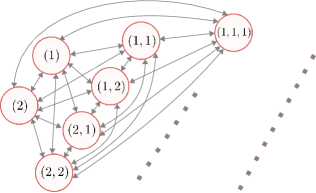
Figure 3: Transition diagram of the sequence-valued discrete-time countable-state Markov chain $\{s(i)\in\mathcal{S}\triangleq\{(1),(2),(1,1),\ldots\}\}_{i\in\mathbb{N}_{0}}$ over the set of mode sequences of variable length

It is important to note that if the set $\{\tau\in\mathbb{N}\,:\,\mu_{\tau}>0\}$ has finite number of elements, then set $\mathcal{S}$ will also contain finite number of sequences. In other words, if the lengths of intervals between mode observation instants have finite number of possible values, then the number of possible sequences is also finite. For example, consider the case where the operation mode of the switched system, which takes values from the index set $\mathcal{M}=\{1,2\}$, is observed periodically with period $2$, that is, $\mu_{2}=1$. In this case, $\mathcal{S}=\{(1,1),(1,2),(2,1),(2,2)\}$ (see Figure 4).

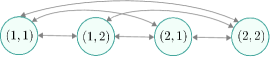
Figure 4: Transition diagram of the sequence-valued discrete-time Markov chain $\{s(i)\in\mathcal{S}\triangleq\{(1,1),(1,2),(2,1),(2,2)\}\}_{i\in\mathbb{N}_{0}}$

We now characterize the initial distribution and the state-transition probabilities of the discrete-time Markov chain $\{s(i)\in\mathcal{S}\}_{i\in\mathbb{N}_{0}}$ as functions of the initial distribution and the state-transition probabilities of the mode signal $\{r(k)\in\mathcal{M}\}_{k\in\mathbb{N}_{0}}$. Specifically, the initial distribution $\lambda:\mathcal{S}\to[0,1]$ of the Markov chain $\{s(i)\in\mathcal{S}\}_{i\in\mathbb{N}_{0}}$ is given by

$$\lambda_{q} =\mathbb{P}[s(0)=q]$$

$$=\mathbb{P}[t_{1}=|q|,r(0)=q_{1},\ldots,r(|q|-1)=q_{|q|}]$$

$$=\mathbb{P}[t_{1}=|q|\,\,\big{|}\,\,r(0)=q_{1},\ldots,r(|q|-1)=q_{|q|}]$$

$$\quad\cdot\mathbb{P}[r(0)=q_{1},\ldots,r(|q|-1)=q_{|q|}],\,\,q\in\mathcal{S}.$$ (10)

Since the mode signal $\{r(k)\in\mathcal{M}\}_{k\in\mathbb{N}_{0}}$ and the mode observation counting process $\{N(k)\in\mathbb{N}_{0}\}_{k\in\mathbb{N}_{0}}$ are mutually independent, mode transitions and mode observations occur independently. Hence, $t_{1}=\tau_{1}$ is independent of $r(n)$ for every $n\in\mathbb{N}_{0}$. As a consequence,

$$\lambda_{q} =\mathbb{P}[t_{1}=|q|]\,\mathbb{P}[r(0)=q_{1},\ldots,r(|q|-1)=q_{|q|}]$$

$$=\mathbb{P}[t_{1}=|q|]\,\mathbb{P}[r(0)=q_{1}]$$

$$\quad\cdot\prod_{n=1}^{|q|-1}\mathbb{P}[r(n)=q_{n+1}|r(n-1)=q_{n}]$$

$$=\begin{cases}\mu_{|q|}\prod_{n=1}^{|q|-1}p_{q_{n},q_{n+1}},&\quad\mathrm{if}\,\,q_{1}=r_{0},\,\,q\in\mathcal{S},\\ 0,&\quad\mathrm{otherwise}.\end{cases}$$ (11)

Note that $s_{1}(0)$, which is the first element of the first mode sequence $s(0)$, is equal to the initial mode $r_{0}$.

Probability of a transition from a mode sequence $q\in\mathcal{S}$ to another mode sequence $\bar{q}\in\mathcal{S}$ is given by

$$\rho_{q,\bar{q}} =\mathbb{P}[s(i+1)=\bar{q}|s(i)=q],$$

$$=\mathbb{P}\big{[}\tau_{i+1}=|\bar{q}|,r(t_{i+1})=\bar{q}_{1},\ldots,$$

$$\quad\quad r(t_{i+1}+|\bar{q}|-1)=\bar{q}_{|\bar{q}|}\,\big{|}\,\tau_{i}=|q|,$$

$$\quad\quad r(t_{i})=q_{1},\ldots,r(t_{i}+|q|-1)=q_{|q|}\big{]},$$ (12)

for $i\in\mathbb{N}_{0}$. Note that $\tau_{i+1}$ is independent of the random variables $r(n),\,n\in\mathbb{N}_{0}$, and $\tau_{i}$. Furthermore, given $r(t_{i}+\tau_{i}-1)$, the random variable $r(t_{i+1})$ is conditionally independent of $r(t_{i}),\ldots,r(t_{i}+\tau_{i}-2)$, and $\tau_{i}$. It follows that

$$\rho_{q,\bar{q}} =\mathbb{P}\big{[}\tau_{i+1}=|\bar{q}|,r(t_{i+1})=\bar{q}_{1},\ldots,$$

$$\quad\quad r(t_{i+1}+|\bar{q}|-1)=\bar{q}_{|\bar{q}|}\,\big{|}\,r(t_{i}+|q|-1)=q_{|q|}\big{]}$$

$$=\mathbb{P}[r(t_{i+1})=\bar{q}_{1}\,|\,r(t_{i}+|q|-1)=q_{|q|}]\mathbb{P}[\tau_{i+1}=|\bar{q}|]$$

$$\,\,\,\,\,\,\cdot\prod_{n=1}^{|\bar{q}|-1}\mathbb{P}[r(t_{i+1}+n)=\bar{q}_{n+1}|r(t_{i+1}+n-1)=\bar{q}_{n}]$$

$$\,=p_{q_{|q|},\bar{q}_{1}}\,\,\,\mu_{|\bar{q}|}\,\prod_{n=1}^{|\bar{q}|-1}p_{\bar{q}_{n},\bar{q}_{n+1}},\quad i\in\mathbb{N}_{0}.$$ (13)

Note that $\mu_{|\bar{q}|}$ in (13) represents the probability that length of the interval between two mode observation instants is equal to the length of the sequence $\bar{q}$, whereas $p_{q_{|q|},\bar{q}_{1}}\in[0,1]$ represents the transition probability from the mode represented by the last element of sequence $q$, to the mode represented by the first element of the sequence $\bar{q}$. Furthermore, the expression $\prod_{n=1}^{|\bar{q}|-1}p_{\bar{q}_{n},\bar{q}_{n+1}}$ denotes the joint probability that the active mode takes the values denoted by the elements of the sequence $\bar{q}$ until the next mode observation instant.

Since the mode signal $\{r(k)\in\mathcal{M}\}_{k\in\mathbb{N}_{0}}$ is aperiodic and irreducible, mode sequences may start with any of the possible modes indicated by the index set $\mathcal{M}=\{1,\ldots,M\}$. Furthermore, it is possible to reach from any mode sequence to another mode sequence in a finite number of mode observations. Hence, the discrete-time Markov chain $\{s(i)\in\mathcal{S}\}_{i\in\mathbb{N}_{0}}$ is irreducible. In Lemma 1 below, we provide the invariant distribution for the countable-state discrete-time Markov chain $\{s(i)\in\mathcal{S}\}_{i\in\mathbb{N}_{0}}$. Note that the distribution $\phi:\mathcal{S}\to[0,1]:j\mapsto\phi_{j}$ is called invariant distribution of the Markov chain $\{s(i)\in\mathcal{S}\}_{i\in\mathbb{N}_{0}}$ if $\phi_{j}=\sum_{i\in\mathcal{S}}\phi_{i}\rho_{i,j}$, $j\in\mathcal{S}$. The invariant distribution for the case where $\mathcal{S}$ contains only sequences of fixed length $T\in\mathbb{N}$ is provided in ?. In Lemma 1, we consider the more general case where $\mathcal{S}$ may contain countably infinite number of sequences of all possible lengths.

Lemma 1.

Discrete-time Markov chain $\{s(i)\in\mathcal{S}\}_{i\in\mathbb{N}_{0}}$ has invariant distribution $\phi:\mathcal{S}\to[0,1]:q\mapsto\phi_{q}$ given by

$$\phi_{q} \triangleq\pi_{q_{1}}\mu_{|q|}\prod_{n=1}^{|q|-1}p_{q_{n},q_{n+1}},\quad q\in\mathcal{S},$$ (14)

where $\pi:\mathcal{M}\to[0,1]$ and $p_{i,j}$, $i,j\in\mathcal{M}$, respectively denote the invariant distribution and transition probabilities of the finite-state Markov chain $\{r(k)\in\mathcal{M}\}_{k\in\mathbb{N}_{0}}$.

Proof 3.1.

We prove this result by showing that $\phi_{\bar{q}}=\sum_{q\in\mathcal{S}}\phi_{q}\rho_{q,\bar{q}}$, for all $\bar{q}\in\mathcal{S}$. First, by (13) and (14)

$$\sum_{q\in\mathcal{S}}\phi_{q}\rho_{q,\bar{q}} =\big{(}\sum_{q\in\mathcal{S}}\pi_{q_{1}}\mu_{|q|}\big{(}\prod_{n=1}^{|q|-1}p_{q_{n},q_{n+1}}\big{)}p_{q_{|q|},\bar{q}_{1}}\big{)}$$

$$\quad\cdot\mu_{|\bar{q}|}\,\prod_{n=1}^{|\bar{q}|-1}p_{\bar{q}_{n},\bar{q}_{n+1}},\quad\bar{q}\in\mathcal{S}.$$ (15)

Now let $\mathcal{S}_{\tau}\triangleq\{q\in\mathcal{S}\,:\,|q|=\tau\},$ $\tau\in\mathbb{N}$. Note that the set $\mathcal{S}_{\tau}$ contains all mode sequences of length $\tau$. We rewrite the sum in (15) to obtain

$$\sum_{q\in\mathcal{S}}\pi_{q_{1}}\mu_{|q|}\big{(}\prod_{n=1}^{|q|-1}p_{q_{n},q_{n+1}}\big{)}p_{q_{|q|},\bar{q}_{1}}$$

$$\,=\sum_{\tau\in\mathbb{N}}\mu_{\tau}\sum_{q\in\mathcal{S}_{\tau}}\pi_{q_{1}}\big{(}\prod_{n=1}^{\tau-1}p_{q_{n},q_{n+1}}\big{)}p_{q_{\tau},\bar{q}_{1}}$$

$$\,=\sum_{\tau\in\mathbb{N}}\mu_{\tau}\sum_{q_{\tau}\in\mathcal{M}}\cdots\sum_{q_{1}\in\mathcal{M}}\pi_{q_{1}}\big{(}\prod_{n=1}^{\tau-1}p_{q_{n},q_{n+1}}\big{)}p_{q_{\tau},\bar{q}_{1}}.$$ (16)

Note that since $\pi:\mathcal{M}\to[0,1]$ is the invariant distribution of the finite-state Markov chain $\{r(k)\in\mathcal{M}\}_{k\in\mathbb{N}_{0}}$, it follows that $\sum_{i\in\mathcal{M}}\pi_{i}p_{i,j}=\pi_{j}$, $i,j\in\mathcal{M}$. Thus, we have $\sum_{q_{n}\in\mathcal{M}}\pi_{q_{n}}p_{q_{n},q_{n+1}}=\pi_{q_{n+1}}$, $n\in\{1,\ldots,\tau-1\}$, and $\sum_{q_{\tau}\in\mathcal{M}}\pi_{q_{\tau}}p_{q_{\tau},\bar{q}_{1}}=\pi_{\bar{q}_{1}}$. As a result, from (16) we obtain

$$\sum_{q\in\mathcal{S}}\pi_{q_{1}}\mu_{|q|}\big{(}\prod_{n=1}^{|q|-1}p_{q_{n},q_{n+1}}\big{)}p_{q_{|q|},\bar{q}_{1}} =\sum_{\tau\in\mathbb{N}}\mu_{\tau}\pi_{\bar{q}_{1}}$$

$$=\pi_{\bar{q}_{1}}.$$ (17)

Finally, substituting (17) into (15) yields

$$\sum_{q\in\mathcal{S}}\phi_{q}\rho_{q,\bar{q}} =\pi_{\bar{q}_{1}}\mu_{|\bar{q}|}\,\prod_{n=1}^{|\bar{q}|-1}p_{\bar{q}_{n},\bar{q}_{n+1}}=\phi_{\bar{q}},\quad\bar{q}\in\mathcal{S},$$ (18)

which completes the proof.

We have now established that the countable-state Markov chain $\{s(k)\in\mathcal{S}\}_{k\in\mathbb{N}_{0}}$ is irreducible and has the invariant distribution $\phi:\mathcal{S}\to[0,1]$ presented in Lemma 1. Note that the strong law of large numbers (also called ergodic theorem; see ?, ?, ?) for discrete-time Markov chains states that $\mathbb{P}[\lim_{n\to\infty}\frac{1}{n}\sum_{k=0}^{n-1}\xi_{s(k)}=\sum_{i\in\mathcal{S}}\phi_{i}\xi_{i}]=1$, for any $\xi_{i}\in\mathbb{R}$, $i\in\mathcal{S}$, such that $\sum_{i\in\mathcal{S}}\phi_{i}|\xi_{i}|<\infty$. This result for the countable-state Markov chain $\{s(k)\in\mathcal{S}\}_{k\in\mathbb{N}_{0}}$ is crucial to obtain the main results of Section 4 below. Specifically, in our stability analysis we utilize the ergodic theorem for Markov chains. In the literature, for the stability analysis of finite-mode (?) and infinite-mode (?) discrete-time switched stochastic systems, researchers employed ergodic theorem for the Markov chain that characterizes the mode signal. In the next section, we use ergodic theorem for the Markov chain that characterizes the sequence of mode values between consecutive mode observation instants.

4 Sufficient Conditions for Almost Sure Asymptotic Stabilization

In this section, we employ the results presented in Section 3 to obtain sufficient conditions for almost sure asymptotic stabilization of the closed-loop system (4) under the control law (6).

Theorem 2.

Consider the switched linear stochastic system (4). If there exist matrices $\tilde{R}>0$, $L_{i}\in\mathbb{R}^{m\times n},\,i\in\mathcal{M}$, and scalars $\zeta_{i,j}\in(0,\infty)$, $i,j\in\mathcal{M}$, such that

$$\,0\geq(A_{i}\tilde{R}+B_{i}L_{j})^{\mathrm{T}}\tilde{R}^{-1}$$

$$\,\,\quad\quad\cdot(A_{i}\tilde{R}+B_{i}L_{j})-\zeta_{i,j}\tilde{R},\quad i,j\in\mathcal{M},$$ (19)

$$\sum_{\tau\in\mathbb{N}}\mu_{\tau}\sum_{l=1}^{\tau}\sum_{i,j\in\mathcal{M}}\pi_{i}p_{i,j}^{(l-1)}\ln\zeta_{j,i}<0,$$ (20)

then the control law (6) with the feedback gain matrix

$$K_{\sigma(k)} =L_{\sigma(k)}\tilde{R}^{-1},$$ (21)

guarantees that the zero solution $x(k)\equiv 0$ of the closed-loop system (4) and (6) is asymptotically stable almost surely.

Proof 4.1.

First, we define $V(x)\triangleq x^{\mathrm{T}}Rx$, where $R\triangleq\tilde{R}^{-1}$. It follows from (4) and (6) that for $k\in\mathbb{N}_{0}$,

$$V(x(k+1)) =x^{\mathrm{T}}(k)(A_{r(k)}+B_{r(k)}K_{\sigma(k)})^{\mathrm{T}}R$$

$$\,\,\,\,\,\,\,\,\cdot(A_{r(k)}+B_{r(k)}K_{\sigma(k)})x(k).$$ (22)

We set $L_{j}=K_{j}R^{-1}$, $j\in\mathcal{M}$, and use (19) and (22) to obtain

$$V(x(k+1)) \leq\zeta_{r(k),\sigma(k)}V(x(k))\leq\eta(k)V(x(0)),$$ (23)

for $k\in\mathbb{N}_{0}$, where $\eta(k)\triangleq\prod_{n=0}^{k}\zeta_{r(n),\sigma(n)}$, $k\in\mathbb{N}$. We will first show that $\eta(k)\to 0$ almost surely as $k\to\infty$. Note that $\eta(k)>0$, $k\in\mathbb{N}_{0}$. Then, it follows that

$$\ln\eta(k) =\sum_{n=0}^{k}\ln\zeta_{r(n),\sigma(n)}.$$ (24)

By using the definitions of stochastic processes $\{N(k)\in\mathbb{N}_{0}\}_{k\in\mathbb{N}_{0}}$ and $\{s(i)\in\mathcal{S}\}_{i\in\mathbb{N}_{0}}$, we obtain

$$\ln\eta(k) =\sum_{n=0}^{t_{N(k)}-1}\ln\zeta_{r(n),\sigma(n)}+\sum_{n=t_{N(k)}}^{k}\ln\zeta_{r(n),\sigma(n)}$$

$$=\sum_{i=0}^{N(k)-1}\xi_{s(i)}+\sum_{n=t_{N(k)}}^{k}\ln\zeta_{r(n),\sigma(n)},$$ (25)

where $\xi_{q}\triangleq\sum_{n=1}^{|q|}\ln\zeta_{q_{n},q_{1}}$, $q\in\mathcal{S}$.

Next, in order to evaluate $\lim_{k\to\infty}\frac{1}{k}\ln\eta(k)$, note that $\lim_{k\to\infty}\frac{1}{k}\sum_{n=t_{N(k)}}^{k}\ln\zeta_{r(n),\sigma(n)}=0.$ Consequently,

$$\lim_{k\to\infty}\frac{1}{k}\ln\eta(k) =\lim_{k\to\infty}\frac{1}{k}\sum_{i=0}^{N(k)-1}\xi_{s(i)}$$

$$=\lim_{k\to\infty}\frac{N(k)}{k}\frac{1}{N(k)}\sum_{i=0}^{N(k)-1}\xi_{s(i)}.$$ (26)

It follows from strong law of large numbers for renewal processes (Section 2.1) that $\lim_{k\to\infty}\frac{N(k)}{k}=\frac{1}{\hat{\tau}}$, where $\hat{\tau}=\sum_{\tau\in\mathbb{N}}\tau\mu_{\tau}$. Furthermore, by the ergodic theorem for countable-state Markov chains, it follows that $\lim_{n\to\infty}\frac{1}{n}\sum_{i=0}^{n-1}\xi_{s(i)}=\sum_{q\in\mathcal{S}}\phi_{q}\xi_{q}$. Using the invariant distribution $\phi:\mathcal{S}\to[0,1]$ given by (14), we get

$$\lim_{k\to\infty}\frac{1}{k}\ln\eta(k)$$

$$\quad=\frac{1}{\hat{\tau}}\sum_{q\in\mathcal{S}}\big{(}\pi_{q_{1}}\mu_{|q|}\prod_{n=1}^{|q|-1}p_{q_{n},q_{n+1}}\big{)}\sum_{m=1}^{|q|}\ln\zeta_{q_{m},q_{1}}.$$ (27)

Let $\mathcal{S}_{\tau}\triangleq\{q\in\mathcal{S}\,:\,|q|=\tau\},\,\tau\in\mathbb{N}$. Note that $\mathcal{S}_{\tau}$ contains all mode sequences of length $\tau$. It follows from (27) that

$$\lim_{k\to\infty}\frac{1}{k}\ln\eta(k)$$

$$\quad=\frac{1}{\hat{\tau}}\sum_{\tau\in\mathbb{N}}\sum_{q\in\mathcal{S}_{\mathrm{\tau}}}\big{(}\pi_{q_{1}}\mu_{|q|}\prod_{n=1}^{|q|-1}p_{q_{n},q_{n+1}}\big{)}\sum_{m=1}^{|q|}\ln\zeta_{q_{m},q_{1}}$$

$$\quad=\frac{1}{\hat{\tau}}\sum_{\tau\in\mathbb{N}}\mu_{\tau}\sum_{q\in\mathcal{S}_{\tau}}\pi_{q_{1}}(\prod_{n=1}^{\tau-1}p_{q_{n},q_{n+1}})\sum_{m=1}^{\tau}\ln\zeta_{q_{m},q_{1}}$$

$$\quad=\frac{1}{\hat{\tau}}\sum_{\tau\in\mathbb{N}}\mu_{\tau}\sum_{m=1}^{\tau}\sum_{q\in\mathcal{S}_{\tau}}\pi_{q_{1}}(\prod_{n=1}^{\tau-1}p_{q_{n},q_{n+1}})\ln\zeta_{q_{m},q_{1}}.$$ (28)

Furthermore, let $\mathcal{S}_{\tau,l}^{i,j}\triangleq\{q\in\mathcal{S}_{\tau}:q_{1}=i,q_{l}=j\}$, $i,j\in\mathcal{M}$, $l\in\{1,2,\ldots,\tau-1\}$. The set $\mathcal{S}_{\tau,l}^{i,j}$ contains all mode sequences of length $\tau$ that have $i\in\mathcal{M}$ and $j\in\mathcal{M}$ as the $1$st and the $l$th elements, respectively. We use (5) to obtain

$$\sum_{q\in\mathcal{S}_{\tau}}\pi_{q_{1}}(\prod_{n=1}^{\tau-1}p_{q_{n},q_{n+1}})\ln\zeta_{q_{l},q_{1}}$$

$$\quad=\sum_{i,j\in\mathcal{M}}\sum_{q\in\mathcal{S}_{\tau,l}^{i,j}}\pi_{q_{1}}(\prod_{n=1}^{\tau-1}p_{q_{n},q_{n+1}})\ln\zeta_{q_{l},q_{1}}$$

$$\quad=\sum_{i,j\in\mathcal{M}}\pi_{i}(\ln\zeta_{j,i})\sum_{q\in\mathcal{S}_{\tau,l}^{i,j}}(\prod_{n=1}^{\tau-1}p_{q_{n},q_{n+1}})$$

$$\quad=\sum_{i,j\in\mathcal{M}}\pi_{i}(\ln\zeta_{j,i})p_{i,j}^{(l-1)}.$$ (29)

Substituting (29) into (28) yields

$$\lim_{k\to\infty}\frac{1}{k}\ln\eta(k) =\frac{1}{\hat{\tau}}\sum_{\tau\in\mathbb{N}}\mu_{\tau}\sum_{l=1}^{\tau}\sum_{i,j\in\mathcal{M}}\pi_{i}p_{i,j}^{(l-1)}\ln\zeta_{j,i}.$$ (30)

Now, since $\hat{\tau}=\sum_{\tau\in\mathbb{N}}\tau\mu_{\tau}<\infty$, as a result of (20), we have $\lim_{k\to\infty}\frac{1}{k}\ln\eta(k)<0$. Thus, $\lim_{k\to\infty}\ln\eta(k)=-\infty$ almost surely; furthermore, $\mathbb{P}[\lim_{k\to\infty}\eta(k)=0]=1.$ In the following, we first show that the zero solution is almost surely stable. To this end first note that for all $\epsilon>0$, $\lim_{n\to\infty}\mathbb{P}[\sup_{k\geq n}\eta(k)>\epsilon^{2}]=0,$ which implies that for all $\epsilon>0$ and $\rho>0$, there exists a positive integer $N(\epsilon,\rho)$ such that $\mathbb{P}[\sup_{k\geq n}\eta(k)>\epsilon^{2}]<\rho$ for $n\geq N(\epsilon,\rho)$. Equivalently,

$$\mathbb{P}[\sup_{k\geq n}\eta(k-1)>\epsilon^{2}]<\rho,\quad n\geq N(\epsilon,\rho)+1.$$ (31)

By the definition of $V(\cdot)$ and (23), we obtain $\eta(k-1)\geq\frac{V(x(k))}{V(x(0))}\geq\frac{\lambda_{\min}(R)}{\lambda_{\max}(R)}\frac{\|x(k)\|^{2}}{\|x(0)\|^{2}}$ for all $k\in\mathbb{N}$. Hence, it follows from (31) that, for all $\epsilon>0$ and $\rho>0$, there exists a positive integer $N(\epsilon,\rho)$ such that

$$\mathbb{P}[\sup_{k\geq n}\|x(k)\|>\epsilon\sqrt{\frac{\lambda_{\max}(R)}{\lambda_{\min}(R)}}\|x(0)\|]$$

$$\quad=\mathbb{P}[\sup_{k\geq n}\|x(k)\|^{2}>\epsilon^{2}\frac{\lambda_{\max}(R)}{\lambda_{\min}(R)}\|x(0)\|^{2}]$$

$$\quad=\mathbb{P}[\sup_{k\geq n}\frac{\lambda_{\min}(R)}{\lambda_{\max}(R)}\frac{\|x(k)\|^{2}}{\|x(0)\|^{2}}>\epsilon^{2}]$$

$$\quad\leq\mathbb{P}[\sup_{k\geq n}\eta(k-1)>\epsilon^{2}]<\rho,\quad n\geq N(\epsilon,\rho)+1.$$ (32)

Let $\delta_{1}\triangleq\sqrt{\frac{\lambda_{\min}(R)}{\lambda_{\max}(R)}}$. If $\|x(0)\|\leq\delta_{1}$, then

$$\mathbb{P}[\sup_{k\geq n}\|x(k)\|>\epsilon]$$

$$\quad\leq\mathbb{P}[\sup_{k\geq n}\|x(k)\|>\epsilon\sqrt{\frac{\lambda_{\max}(R)}{\lambda_{\min}(R)}}\|x(0)\|]$$

$$\quad<\rho,\quad n\geq N(\epsilon,\rho)+1.$$ (33)

Now let $\bar{\zeta}\triangleq\max\{1,\max_{i,j\in\mathcal{M}}\zeta_{i,j}\}$. It follows from (23) that $V(x(k))\leq\bar{\zeta}^{k-1}V(x(0))\leq\bar{\zeta}^{N(\epsilon,\rho)-1}V(x(0))$ for all $k\in\{0,1,\ldots,N(\epsilon,\rho)\}$. Therefore, $\|x(k)\|^{2}\leq\bar{\zeta}^{N(\epsilon,\rho)-1}\frac{\lambda_{\max}(R)}{\lambda_{\min}(R)}\|x(0)\|^{2}$, and hence, we have $\|x(k)\|\leq\sqrt{\bar{\zeta}^{N(\epsilon,\rho)-1}\frac{\lambda_{\max}(R)}{\lambda_{\min}(R)}}\|x(0)\|,$ for all $k\in\{0,1,\ldots,N(\epsilon,\rho)\}$. Furthermore, let $\delta_{2}\triangleq\epsilon\sqrt{\bar{\zeta}^{-N(\epsilon,\rho)+1}\frac{\lambda_{\min}(R)}{\lambda_{\max}(R)}}$. Consequently, if $\|x(0)\|\leq\delta_{2}$, then $\|x(k)\|\leq\epsilon$, $k\in\{0,1,\ldots,N(\epsilon,\rho)\}$, which implies

$$\mathbb{P}[\max_{k\in\{0,1,\ldots,N(\epsilon,\rho)\}}\|x(k)\|>\epsilon] = 0.$$ (34)

It follows from (33) and (34) that for all $\epsilon>0$, $\rho>0$,

$$\mathbb{P}[\sup_{k\in\mathbb{N}_{0}}\|x(k)\|>\epsilon] =\mathbb{P}[\{\max_{k\in\{0,1,\ldots,N(\epsilon,\rho)\}}\|x(k)\|>\epsilon\}$$

$$\quad\quad\cup\,\{\sup_{k\geq N(\epsilon,\rho)+1}\|x(k)\|>\epsilon\}]$$

$$\leq\mathbb{P}[\max_{k\in\{0,1,\ldots,N(\epsilon,\rho)\}}\|x(k)\|>\epsilon]$$

$$\quad+\mathbb{P}[\sup_{k\geq N(\epsilon,\rho)+1}\|x(k)\|>\epsilon]$$

$$<\rho,$$ (35)

whenever $\|x(0)\|<\delta\triangleq\min(\delta_{1},\delta_{2})$, which implies almost sure stability. As a final step of proving almost sure asymptotic stability of the zero solution, we now show (3). First, note that by (23), we have $V(x(k+1))\leq\eta(k)V(x(0))$, $k\in\mathbb{N}$. Now, since $\mathbb{P}[\lim_{k\to\infty}\eta(k)=0]=1$, it follows that $\mathbb{P}[\lim_{k\to\infty}V(x(k))=0]=1$, which implies (3), and hence the zero solution of the closed-loop system (4), (6) is asymptotically stable almost surely.

Theorem 2 provides sufficient conditions for almost sure asymptotic stability of the closed-loop system (4) and (6). Conditions (19) and (20) of Theorem 2 indicate dependence of stabilization performance on subsystem dynamics, mode transition probabilities, and random mode observations. The effect of mode transitions on the stabilization is reflected in (19) through the limiting distribution $\pi:\mathcal{M}\to[0,1]$ as well as $l$-step transition probabilities $p_{i,j}^{(l)}$, $i,j\in\mathcal{M}$. Furthermore, the effect of random mode observations is indicated in condition (19) by $\mu:\mathbb{N}\to[0,1]$, which represents the distribution of the lengths of intervals between consecutive mode observation instants.

Remark 3.

We investigate the stability of the closed-loop system through the Lyapunov-like function $V(x)\triangleq x^{\mathrm{T}}Rx$ with $R=\tilde{R}^{-1}$, where $\tilde{R}$ is a positive-definite matrix that satisfy (19). The scalar $\zeta_{i,j}\in(0,\infty)$ in (19) characterizes an upper bound on the growth of the Lyapunov-like function, when the switched system evolves according to dynamics of the $i$th subsystem and the $j$th feedback gain. Note that if $\zeta_{i,j}\in(0,1)$ for all $i,j\in\mathcal{M}$, it is guaranteed that the Lyapunov-like function will decrease at each time step. However, we do not require $\zeta_{i,j}\in(0,1)$ for all $i,j\in\mathcal{M}$. There may be pairs $i,j\in\mathcal{M}$ such that $\zeta_{i,j}>1$, hence Lyapunov-like function $V(\cdot)$ may grow when $i$th subsystem and the $j$th feedback gain is active. As long as $\zeta_{i,j}$, $i,j\in\mathcal{M}$, satisfy (20) the Lyapunov-like is guaranteed to converge to zero in the long-run (even if it may grow at certain instants). Note that even though the conditions (19), (20) allow unstable subsystem-feedback gain pairs, some conservativeness may still arise due the characterization with single Lyapunov-like function. This conservatism may be reduced with an alternative approach with multiple Lyapunov-like functions assigned for each subsystem-feedback gain pairs.

Remark 4.

In order to verify conditions (19) and (20) of Theorem 2, we take an approach similar to the one presented in ?. Specifically, we use Schur complements (see ?) to transform condition (19) into the matrix inequalities

$$0\leq \left[\begin{array}[]{cc}\zeta_{i,j}\tilde{R}&\hat{A}_{i,j}^{\mathrm{T}}\\ \hat{A}_{i,j}&\tilde{R}\end{array}\right],\quad i,j\in\mathcal{M},$$ (38)

where $\hat{A}_{i,j}\triangleq(A_{i}\tilde{R}+B_{i}L_{j}),\,i,j\in\mathcal{M}$. Note that the inequalities (38) are linear in $\tilde{R}$ and $L_{i}$, $i\in\mathcal{M}$. In our numerical method, we iterate over a set of the values of $\zeta_{i,j}$, $i,j\in\mathcal{M}$, that satisfy (20) and at each iteration we look for feasible solutions to the linear matrix inequalities (38). In Section 5 below, we employ this method and find values for matrices $\tilde{R}\in\mathbb{R}^{n\times n},L_{i}\in\mathbb{R}^{m\times n},i\in\mathcal{M}$, and scalars $\zeta_{i,j}\in(0,\infty),i,j\in\mathcal{M}$, that satisfy (19), (20) for a given discrete-time switched linear system. It is important to note that the scalars $\zeta_{i,j}\in(0,\infty),i,j\in\mathcal{M}$, that satisfy (20) form an unbounded set. Note that this set is smaller than the entire nonnegative orthant in $\mathbb{R}^{M^{2}}$. However, we still need to reduce the search space of $\zeta_{i,j},i,j\in\mathcal{M}$. To this end, first note that it is harder to find feasible solutions to linear matrix inequalities given by (38) when the scalars $\zeta_{i,j},i,j\in\mathcal{M},$ are close to zero. Note also that if there exist a feasible solution to (38) for certain values of $\zeta_{i,j},i,j\in\mathcal{M},$ then it is guaranteed that feasible solutions to (38) exist also for larger values of $\zeta_{i,j},i,j\in\mathcal{M}$. Therefore, we can restrict our search space and iterate over large values of $\zeta_{i,j},i,j\in\mathcal{M},$ that satisfy (20), and check feasible solutions to (38). Specifically, we only iterate over $\zeta_{i,j},i,j\in\mathcal{M},$ that is close to the search space’s boundary identified by $\sum_{\tau\in\mathbb{N}}\mu_{\tau}\sum_{l=1}^{\tau}\sum_{i,j\in\mathcal{M}}\pi_{i}p_{i,j}^{(l-1)}\ln\zeta_{j,i}=0$. Now note that in order for (20) to be satisfied, there must exist at least a pair $i,j\in\mathcal{M}$ such that $\zeta_{i,j}<1$. Since the scalar $\zeta_{i,j}$ represents the stability/instability margin for the dynamics characterized by the $i$th subsystem and the $j$th feedback gain, we expect $\zeta_{i,i}<1$ for stabilizable modes $i\in\mathcal{M}$. This further reduces the search space for our numerical method.

Remark 5.

Note that conditions (19) and (20) presented in Theorem 2 can also be used for determining almost sure asymptotic stability of the switched stochastic control system (4), (6) with periodically observed mode information. The renewal process characterization presented in this paper in fact encompasses periodic mode observations (explored previously in ? and ?) as a special case. Specifically, suppose that the mode observation instants are given by $t_{i}=iT$, $i\in\mathbb{N}_{0}$, where $T\in\mathbb{N}$ denotes the mode observation period. Our present framework allows us to characterize periodic mode observations by setting the distribution $\mu:\mathbb{N}\to[0,1]$ such that $\mu_{T}=1$ and $\mu_{\tau}=0$, $\tau\neq T$. Note that condition (20) of Theorem 2 for this case reduces to $\sum_{l=1}^{T}\sum_{i,j\in\mathcal{M}}\pi_{i}p_{i,j}^{(l-1)}\ln\zeta_{j,i}<0$. Furthermore, if the controller has perfect mode information at all time instants ($T=1$, hence $\sigma(k)=r(k)$, $k\in\mathbb{N}_{0}$), condition (20) takes even a simpler form given by the inequality $\sum_{i\in\mathcal{M}}\pi_{i}\ln\zeta_{i,i}<0$.

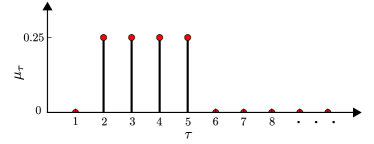
Figure 5: Uniform distribution given by (39) with $\tau_{L}=2$ and $\tau_{H}=5$ for the length of intervals between consecutive mode observation instants

Remark 6.

Condition (20) of Theorem 2 has a simpler form also for the case where the length of intervals between consecutive mode observation instants are uniformly distributed over the set $\{\tau_{\mathrm{L}},\tau_{\mathrm{L}}+1,\ldots,\tau_{\mathrm{H}}\}$ with $\tau_{\mathrm{L}},\tau_{\mathrm{H}}\in\mathbb{N}$ such that $\tau_{\mathrm{L}}\leq\tau_{\mathrm{H}}$. In this case the distribution $\mu:\mathbb{N}\to[0,1]$ is given by

$$\mu_{\tau} \triangleq\begin{cases}\frac{1}{\tau_{\mathrm{H}}-\tau_{\mathrm{L}}+1},&\quad\mathrm{if}\,\,\,\tau\in\{\tau_{\mathrm{L}},\tau_{\mathrm{L}}+1,\ldots,\tau_{\mathrm{H}}\},\\ 0,&\quad\mathrm{otherwise}.\end{cases}$$ (39)

Figure 5 shows the distribution (39) for an example case with $\tau_{\mathrm{L}}=2$ and $\tau_{\mathrm{H}}=5$.

With (39), condition (20) of Theorem 2 reduces to the inequality $\sum_{\tau=\tau_{\mathrm{L}}}^{\tau_{\mathrm{H}}}\sum_{l=1}^{\tau}\sum_{i,j\in\mathcal{M}}\pi_{i}p_{i,j}^{(l-1)}\ln\zeta_{j,i}<0.$

Remark 7.

Note that our probabilistic characterization of mode observation instants also allows us to explore the feedback control problem under missing mode samples. Specifically, consider the case where the mode is sampled at all time instants; however, some of the mode samples are lost during communication between mode sampling mechanism and the controller. Suppose that the controller receives a sampled mode data at each time step $k\in\mathbb{N}$ with probability $\theta\in(0,1)$. In other words, the mode data is lost with probability $1-\theta$. We investigate this problem by setting

$$\mu_{\tau} \triangleq(1-\theta)^{\tau-1}\theta,\quad\tau\in\mathbb{N}.$$ (40)

Figure 6 shows the distribution (40) with $\theta=0.3$.

It turns out that for $\mu_{\tau}:\mathbb{N}\to[0,1]$ given by (40), the left-hand side of condition (20) has a closed-form expression. Note that by changing the order of summations and using (40), we can rewrite the left-hand side of (20) as

$$\sum_{\tau\in\mathbb{N}}\mu_{\tau}\sum_{l=1}^{\tau}\sum_{i,j\in\mathcal{M}}\pi_{i}p_{i,j}^{(l-1)}\ln\zeta_{j,i}$$

$$\,\,=\sum_{i,j\in\mathcal{M}}\pi_{i}(\ln\zeta_{j,i})\sum_{\tau\in\mathbb{N}}\mu_{\tau}\sum_{l=1}^{\tau}p_{i,j}^{(l-1)}$$

$$\,\,=\sum_{i,j\in\mathcal{M}}\pi_{i}(\ln\zeta_{j,i})\sum_{l=1}^{\infty}p_{i,j}^{(l-1)}\sum_{\tau=l}^{\infty}\mu_{\tau}$$

$$\,\,=\sum_{i,j\in\mathcal{M}}\pi_{i}(\ln\zeta_{j,i})\sum_{l=1}^{\infty}p_{i,j}^{(l-1)}(1-\sum_{\tau=1}^{l-1}\mu_{\tau})$$

$$\,\,=\sum_{i,j\in\mathcal{M}}\pi_{i}(\ln\zeta_{j,i})\sum_{l=1}^{\infty}p_{i,j}^{(l-1)}\big{(}1-\sum_{\tau=1}^{l-1}(1-\theta)^{\tau-1}\theta\big{)}.$$ (41)

Note that $\big{(}1-\sum_{\tau=1}^{l-1}(1-\theta)^{\tau-1}\theta\big{)}=\big{(}1-\theta\frac{1-(1-\theta)^{l-1}}{1-(1-\theta)}\big{)}=(1-\theta)^{l-1}$. Therefore,

$$\sum_{\tau\in\mathbb{N}}\mu_{\tau}\sum_{l=1}^{\tau}\sum_{i,j\in\mathcal{M}}\pi_{i}p_{i,j}^{(l-1)}\ln\zeta_{j,i}$$

$$\quad=\sum_{i,j\in\mathcal{M}}\pi_{i}(\ln\zeta_{j,i})\sum_{l=1}^{\infty}p_{i,j}^{(l-1)}(1-\theta)^{l-1}.$$ (42)

Let $Z\triangleq\sum_{l=1}^{\infty}P^{l-1}(1-\theta)^{l-1},$ where $P\in\mathbb{R}^{M\times M}$ denotes the transition probability matrix for the mode signal $\{r(k)\in\mathcal{M}\}_{k\in\mathbb{N}_{0}}$. Note that the infinite sum in the definition of $Z$ converges, because the eigenvalues of the matrix $(1-\theta)P$ are strictly inside the unit circle of the complex plane. By using the formula for geometric series of matrices (?), we obtain $Z=\big{(}I-(1-\theta)P)^{-1}$. Furthermore, it follows from (42) that $\sum_{\tau\in\mathbb{N}}\mu_{\tau}\sum_{l=1}^{\tau}\sum_{i,j\in\mathcal{M}}\pi_{i}p_{i,j}^{(l-1)}\ln\zeta_{j,i}=\sum_{i,j\in\mathcal{M}}\pi_{i}(\ln\zeta_{j,i})z_{i,j}$, and therefore, when $\mu:\mathbb{N}\to[0,1]$ is given by (40), condition (20) takes the form $\sum_{i,j\in\mathcal{M}}\pi_{i}(\ln\zeta_{j,i})z_{i,j}<0$, where $z_{i,j}$ is the $(i,j)$th entry of the matrix $Z$.

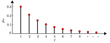
Figure 6: Distribution given by (40) with $\theta=0.3$ for the length of intervals between consecutive mode observation instants

Remark 8.

Note that in order to check condition (20) of Theorem 2, one needs to have perfect information regarding the distribution $\mu:\mathbb{N}\to[0,1]$, according to which the lengths of intervals between consecutive mode observation instants are distributed. In Theorem 9 below, we present alternative sufficient stabilization conditions, which do not require exact knowledge of $\mu:\mathbb{N}\to[0,1]$. Specifically, we consider the case where the mode observation instants $t_{i}$, $i\in\mathbb{N}_{0}$, satisfy

$$\mathbb{P}[t_{i+1}-t_{i}\leq\bar{\tau}] =1,\quad i\in\mathbb{N}_{0},$$ (43)

where $\bar{\tau}\in\mathbb{N}$ is a known constant. In this case time instants of consecutive mode observations are assumed to be at most $\bar{\tau}\in\mathbb{N}$ steps apart. In other words, if (43) is satisfied, it is guaranteed that the length of intervals between consecutive mode observation instants cannot be larger than $\bar{\tau}\in\mathbb{N}$. It is important to note that (43) characterizes a requirement on the intervals between mode observation instants and it is not related to mode switches.

Theorem 9.

Consider the switched linear stochastic system (4). Suppose that the mode-transition probability matrix $P\in\mathbb{R}^{M\times M}$ possesses only positive real eigenvalues. If there exist matrices $\tilde{R}>0$, $L_{i}\in\mathbb{R}^{m\times n},\,i\in\mathcal{M}$, and scalars $\bar{\tau}\in\mathbb{N}$, $\zeta_{i,j}\in(0,\infty)$, $i,j\in\mathcal{M}$, such that (19), (43),

$$\,\,\,\,0\leq\zeta_{j,i}-\zeta_{i,i},\quad i,j\in\mathcal{M},$$ (44)

$$\sum_{l=1}^{\bar{\tau}}\sum_{i,j\in\mathcal{M}}\pi_{i}p_{i,j}^{(l-1)}\ln\zeta_{j,i}<0,$$ (45)

hold, then the control law (6) with the feedback gain matrix (21) guarantees that the zero solution $x(k)\equiv 0$ of the closed-loop system is asymptotically stable almost surely.

Proof 4.2.

The mode signal $\{r(k)\in\mathcal{M}\}_{k\in\mathbb{N}_{0}}$ is an irreducible and aperiodic Markov chain; therefore, the invariant distribution $\pi:\mathcal{M}\to[0,1]$ is also the limiting distribution (?). Thus, for all $i,j\in\mathcal{M}$ and $k\in\mathbb{N}_{0}$,

$$\lim_{l\to\infty}p_{i,j}^{(l)} =\lim_{l\to\infty}\mathbb{P}[r(k+l)=j|r(k)=i]=\pi_{j}.$$ (46)

Now, let $p_{i}^{(l)}\in[0,1]^{1\times M}$,$i\in\mathcal{M}$, denote the row vector with the $j$th element given by the $l$-step transition probability $p_{i,j}^{(l)}$. Note that $p_{i}^{(\cdot)}$ is the unique solution of the difference equation

$$p_{i}^{(l+1)} =p_{i}^{(l)}P,\quad l\in\mathbb{N}_{0},$$ (47)

with the initial condition $p_{i,i}^{(0)}=1$ and $p_{i,j}^{(0)}=0$, $i\neq j$, $j\in\mathcal{M}$. Since all the eigenvalues of the mode-transition probability matrix $P\in\mathbb{R}^{M\times M}$ are positive real numbers, the solution $p_{i}^{(\cdot)}$ of the difference equation (47) does not comprise any oscillatory components, and $l$-step transition probabilities $p_{i,j}^{(l)}$, $i,j\in\mathcal{M}$, converge towards their limiting values monotonically, that is,

$$p_{i,i}^{(l+1)} \leq p_{i,i}^{(l)},\quad i\in\mathcal{M},\,\,l\in\mathbb{N}_{0},$$ (48)

$$p_{i,j}^{(l+1)} \geq p_{i,j}^{(l)},\quad i\neq j,\,\,\,i,j\in\mathcal{M},\,\,\,l\in\mathbb{N}_{0}.$$ (49)

Now note that for all $i,j\in\mathcal{M}$, and $\tau\in\mathbb{N}$,

$$\frac{1}{\tau}\sum_{l=1}^{\tau}p_{i,j}^{(l-1)} =\frac{1}{\tau+1}\big{(}\sum_{l=1}^{\tau}p_{i,j}^{(l-1)}+\frac{1}{\tau}\sum_{l=1}^{\tau}p_{i,j}^{(l-1)}\big{)}.$$ (50)

By (49), we have $p_{i,j}^{(l-1)}\leq p_{i,j}^{\tau}$, $l\in\{1,2,\ldots,\tau\}$, $i,j\in\mathcal{M}$, $i\neq j$. Hence, it follows from (50) that

$$\frac{1}{\tau}\sum_{l=1}^{\tau}p_{i,j}^{(l-1)} \leq\frac{1}{\tau+1}\big{(}\sum_{l=1}^{\tau}p_{i,j}^{(l-1)}+\frac{1}{\tau}\sum_{l=1}^{\tau}p_{i,j}^{(\tau)}\big{)}$$

$$=\frac{1}{\tau+1}\big{(}\sum_{l=1}^{\tau}p_{i,j}^{(l-1)}+p_{i,j}^{(\tau)}\big{)}$$

$$=\frac{1}{\tau+1}\sum_{l=1}^{\tau+1}p_{i,j}^{(l-1)},\quad\tau\in\mathbb{N},\,\,\,i\neq j.$$ (51)

As a consequence, for all $\tau\leq\bar{\tau}$ it follows that

$$\frac{1}{\tau}\sum_{l=1}^{\tau}p_{i,j}^{(l-1)} \leq\frac{1}{\bar{\tau}}\sum_{l=1}^{\bar{\tau}}p_{i,j}^{(l-1)},\quad i\neq j,\,\,\,i,j\in\mathcal{M}.$$ (52)

Next, we show that (43)–(45) together with (52) imply (20). First, let $\kappa_{\tau,\bar{\tau}}^{i,j}\triangleq\frac{1}{\tau}\sum_{l=1}^{\tau}p_{i,j}^{(l-1)}-\frac{1}{\bar{\tau}}\sum_{l=1}^{\bar{\tau}}p_{i,j}^{(l-1)}$, $i,j\in\mathcal{M}$. It follows that

$$\frac{1}{\tau}\sum_{l=1}^{\tau}\sum_{i,j\in\mathcal{M}}\pi_{i}p_{i,j}^{(l-1)}\ln\zeta_{j,i}$$

$$\quad=\sum_{i,j\in\mathcal{M}}\pi_{i}\ln\zeta_{j,i}\frac{1}{\tau}\sum_{l=1}^{\tau}p_{i,j}^{(l-1)}$$

$$\quad=\sum_{i,j\in\mathcal{M}}\pi_{i}(\ln\zeta_{j,i})\kappa_{\tau,\bar{\tau}}^{i,j}+\frac{1}{\bar{\tau}}\sum_{l=1}^{\bar{\tau}}\sum_{i,j\in\mathcal{M}}\pi_{i}p_{i,j}^{(l-1)}\ln\zeta_{j,i}$$

$$\quad=\sum_{i\in\mathcal{M}}\pi_{i}(\ln\zeta_{i,i})\kappa_{\tau,\bar{\tau}}^{i,i}+\sum_{i\in\mathcal{M}}\sum_{j\in\mathcal{M},j\neq i}\pi_{i}(\ln\zeta_{j,i})\kappa_{\tau,\bar{\tau}}^{i,j}$$

$$\quad\quad+\frac{1}{\bar{\tau}}\sum_{l=1}^{\bar{\tau}}\sum_{i,j\in\mathcal{M}}\pi_{i}p_{i,j}^{(l-1)}\ln\zeta_{j,i}.$$ (53)

Note that by (52), we have $\kappa_{\tau,\bar{\tau}}^{i,j}\leq 0$, $\tau\leq\bar{\tau}$, $i\neq j$. It follows from (44) that, for $\tau\leq\bar{\tau}$,

$$(\ln\zeta_{j,i})\kappa_{\tau,\bar{\tau}}^{i,j} \leq(\ln\zeta_{i,i})\kappa_{\tau,\bar{\tau}}^{i,j},\quad i\neq j,\,\,i,j\in\mathcal{M}.$$ (54)

Now, since $\sum_{j\in\mathcal{M}}p_{i,j}^{(l)}=1$, $l\in\mathbb{N}_{0}$, $i\in\mathcal{M}$, we have

$$\sum_{j\in\mathcal{M}}\kappa_{\tau,\bar{\tau}}^{i,j} =\sum_{j\in\mathcal{M}}\frac{1}{\tau}\sum_{l=1}^{\tau}p_{i,j}^{(l-1)}-\sum_{j\in\mathcal{M}}\frac{1}{\bar{\tau}}\sum_{l=1}^{\bar{\tau}}p_{i,j}^{(l-1)}$$

$$=\frac{1}{\tau}\sum_{l=1}^{\tau}\sum_{j\in\mathcal{M}}p_{i,j}^{(l-1)}-\frac{1}{\bar{\tau}}\sum_{l=1}^{\bar{\tau}}\sum_{j\in\mathcal{M}}p_{i,j}^{(l-1)}$$

$$=\frac{\tau}{\tau}-\frac{\bar{\tau}}{\bar{\tau}}=0,\quad i\in\mathcal{M}.$$ (55)

We use (53)–(55) to obtain

$$\frac{1}{\tau}\sum_{l=1}^{\tau}\sum_{i,j\in\mathcal{M}}\pi_{i}p_{i,j}^{(l)}\ln\zeta_{j,i}$$

$$\quad\leq\sum_{i\in\mathcal{M}}\pi_{i}(\ln\zeta_{i,i})\kappa_{\tau,\bar{\tau}}^{i,j}+\sum_{i\in\mathcal{M}}\sum_{j\in\mathcal{M},j\neq i}\pi_{i}(\ln\zeta_{i,i})\kappa_{\tau,\bar{\tau}}^{i,j}$$

$$\quad\quad+\sum_{i,j\in\mathcal{M}}\pi_{i}(\ln\zeta_{j,i})\frac{1}{\bar{\tau}}\sum_{l=1}^{\bar{\tau}}p_{i,j}^{(l-1)}$$

$$\quad=\sum_{i\in\mathcal{M}}\pi_{i}(\ln\zeta_{i,i})\sum_{j\in\mathcal{M}}\kappa_{\tau,\bar{\tau}}^{i,j}$$

$$\quad\quad+\sum_{i,j\in\mathcal{M}}\pi_{i}(\ln\zeta_{j,i})\frac{1}{\bar{\tau}}\sum_{l=1}^{\bar{\tau}}p_{i,j}^{(l-1)}$$

$$\quad=\frac{1}{\bar{\tau}}\sum_{l=1}^{\bar{\tau}}\sum_{i,j\in\mathcal{M}}\pi_{i}p_{i,j}^{(l-1)}\ln\zeta_{j,i},\quad\tau\leq\bar{\tau}.$$ (56)

Finally, it follows from (43) and (56) that

$$\sum_{\tau\in\mathbb{N}}\mu_{\tau}\sum_{l=1}^{\tau}\sum_{i,j\in\mathcal{M}}\pi_{i}p_{i,j}^{(l-1)}\ln\zeta_{j,i}$$

$$\quad=\sum_{\tau\in\mathbb{N}}\mu_{\tau}\tau\big{(}\frac{1}{\tau}\sum_{l=1}^{\tau}\sum_{i,j\in\mathcal{M}}\pi_{i}p_{i,j}^{(l-1)}\ln\zeta_{j,i}\big{)}$$

$$\quad\leq\sum_{\tau\in\mathbb{N}}\mu_{\tau}\tau\big{(}\frac{1}{\bar{\tau}}\sum_{l=1}^{\bar{\tau}}\sum_{i,j\in\mathcal{M}}\pi_{i}p_{i,j}^{(l-1)}\ln\zeta_{j,i}\big{)}.$$ (57)

Note that (45) and (57) imply (20). Hence, the result follows from Theorem 2.

Conditions of Theorem 9 can be utilized for assessing stability of a switched stochastic control system, even if exact knowledge of the distribution $\mu:\mathbb{N}\to[0,1]$ is not available. Note that the requirement on the knowledge of $\mu:\mathbb{N}\to[0,1]$ is relaxed in Theorem 9 by imposing other conditions on the mode-transition probability matrix $P\in\mathbb{R}^{M\times M}$ and the scalars $\zeta_{i,j}\in(0,\infty)$, $i,j\in\mathcal{M}$.

5 Illustrative Numerical Examples

In this section we provide numerical examples to demonstrate the results presented in this paper.

Example 10.

Consider the switched stochastic system (4) with $M=2$ modes described by the subsystems matrices

$$A_{1}=\left[\begin{array}[]{cc}0&1\\ 1.6&-0.3\end{array}\right] \,,\quad A_{2}=\left[\begin{array}[]{cc}0&1\\ -0.5&1.4\end{array}\right],$$

$B_{1}=[0,\,1]^{\mathrm{T}}$, and $B_{2}=[0,\,-1]^{\mathrm{T}}$. The mode signal $\{r(k)\in\mathcal{M}\triangleq\{1,2\}\}_{k\in\mathbb{N}_{0}}$ of the switched system is assumed to be an aperiodic and irreducible Markov chain characterized by the transition probabilities $p_{1,2}=p_{2,1}=0.3$ and $p_{1,1}=p_{2,2}=0.7$. The invariant distribution for $\{r(k)\in\mathcal{M}\triangleq\{1,2\}\}_{k\in\mathbb{N}_{0}}$ is given by $\pi_{1}=\pi_{2}=0.5$. Moreover, $\mu:\mathbb{N}\to[0,1]$, according to which the lengths of intervals between consecutive mode observation instants are distributed, is assumed to be given by $\mu_{\tau}=(1-\theta)^{\tau-1}\theta$, $\tau\in\mathbb{N}$, with $\theta=0.3$. In this case, at each time step $k\in\mathbb{N}$, the mode may be observed with probability $\theta=0.3$ (see Remark 7).

Note that

$$\tilde{R} =\left[\begin{array}[]{cc}3.0143&-0.1485\\ -0.1485&1.5280\end{array}\right],$$ (60)

$L_{1}=\left[-3.5326\,\,\,0.9608\right]$, $L_{2}=\left[-3.0029\,\,\,1.8284\right]$, and the scalars $\zeta_{1,1}=0.7$, $\zeta_{1,2}=1.8$, $\zeta_{2,1}=2$, and $\zeta_{2,2}=0.8$ satisfy (19) and (20). Now, it follows from Theorem 2 that the proposed control law (6) with feedback gain matrices

$$K_{1} =L_{1}\tilde{R}^{-1}=\left[-1.1465\,\,\,0.5174\right],$$ (61)

$$K_{2} =L_{2}\tilde{R}^{-1}=\left[-0.9718\,\,\,1.1021\right],$$ (62)

guarantees almost sure asymptotic stability of the closed-loop switched stochastic system (4), (6).

Sample paths of the state $x(k)$ and the control input $u(k)$ (obtained with initial conditions $x(0)=\left[1,\,-1\right]^{\mathrm{T}}$ and $r(0)=1$) are shown in Figures 7 and 8. Furthermore, Figure 9 shows a sample path of the actual mode signal $r(k)$ and its sampled version $\sigma(k)$. Figures 7–9 indicate that our proposed control framework guarantees stabilization even for the case where operation mode of the switched system is observed only at random time instants.

Figure 7: State trajectory versus time

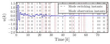
Figure 8: Control input versus time

Figure 9: Actual mode $r(k)$ and sampled mode $\sigma(k)$

The control law (6) with feedback gain matrices (61) and (62) guarantee stabilization of the closed-loop system with random mode observations characterized by distribution $\mu_{\tau}=(1-\theta)^{\tau-1}\theta$ with $\theta=0.3$. Note that for each time step, $\theta$ represents the probability of mode information being available for control purposes. In order to investigate conservativeness of our results, we search all values of parameter $\theta$ for which the control law (6) with feedback gains (61) and (62) achieve stabilization. To this end, first, we search values of $\theta$ such that there exist a positive-definite matrix $\tilde{R}$, and scalars $\zeta_{i,j}$, $i,j\in\mathcal{M}$ that satisfy conditions (19) and (20) of Theorem 2 with $L_{1}=K_{1}\tilde{R}$ and $L_{2}=K_{2}\tilde{R}$, where $K_{1}$ and $K_{2}$ are given by (61) and (62). We find that for parameter values $\theta\in[0.2,1]$, conditions (19) and (20) are satisfied. Hence Theorem 2 guarantees stabilization for the case where parameter $\theta$ is inside the range $[0.2,1]$. On the other hand, through repetitive numerical simulations we observe that the states of the closed-loop system converge to the origin in fact for a larger range of parameter values ($\theta\in[0.12,1]$), which indicate some conservativeness in the conditions of Theorem 2 (see Remark 3).

Example 11.

Consider the switched stochastic system (4) with $M=3$ modes described by the subsystems matrices

$$A_{1}=\left[\begin{array}[]{cc}0&1\\ 1.5&0.5\end{array}\right] ,\,\,\,A_{2}=\left[\begin{array}[]{cc}0&1\\ 1&0.5\end{array}\right],\,\,\,A_{3}=\left[\begin{array}[]{cc}0&-1\\ 1.1&1.2\end{array}\right],$$

$B_{1}=[0,\,1]^{\mathrm{T}}$, $B_{2}=[0,\,0.2]^{\mathrm{T}}$, and $B_{3}=[0,\,0.7]^{\mathrm{T}}$. The mode signal $\{r(k)\in\mathcal{M}\triangleq\{1,2,3\}\}_{k\in\mathbb{N}_{0}}$ of the switched system is assumed to be an aperiodic and irreducible Markov chain characterized by the transition matrix $P$ with entries $p_{i,i}=0.6$, $i\in\mathcal{M}$, and $p_{i,j}=0.2$, $i\neq j$, $i,j\in\mathcal{M}$. The invariant distribution for $\{r(k)\in\mathcal{M}\triangleq\{1,2,3\}\}_{k\in\mathbb{N}_{0}}$ is given by $\pi_{1}=\pi_{2}=\pi_{3}=\frac{1}{3}$. Furthermore, note that the transition matrix $P$ possesses positive real eigenvalues $0.4$ (with algebraic multiplicity $2$) and $1$. The lengths of intervals between consecutive mode observation instants are assumed to be uniformly distributed over the set $\{2,3,4,5\}$ (see Remark 6). In other words, the distribution $\mu:\mathbb{N}\to[0,1]$ is assumed to be given by (39) with $\tau_{\mathrm{L}}=2$ and $\tau_{\mathrm{H}}=5$. Note that for this example the mode observation instants $t_{i}$, $i\in\mathbb{N}_{0}$, satisfy (43) with $\bar{\tau}=5$.

In this example, we will utilize Theorem 9 for the case where the upper-bounding constant $\bar{\tau}=5$ is known, but the exact knowledge of the distribution $\mu:\mathbb{N}\to[0,1]$ is not available (see Remark 9). Specifically, note that

$$\tilde{R} =\left[\begin{array}[]{cc}2.6465&-0.7851\\ -0.7851&1.2568\end{array}\right],$$ (65)

$L_{1}=\left[-3.5858\,\,\,\,\,0.1413\right]$, $L_{2}=\left[-4.7066\,\,\,\,-0.3329\right]$, $L_{3}=\left[-3.2532\,\,\,\,-0.3601\right]$, and the scalars $\zeta_{1,1}=0.6$, $\zeta_{1,2}=1.7$, $\zeta_{1,3}=1.5$, $\zeta_{2,1}=1.6$, $\zeta_{2,2}=0.7$, $\zeta_{2,3}=2$, $\zeta_{3,1}=2$, $\zeta_{3,2}=2$, and $\zeta_{3,3}=0.5$ satisfy (19), (44), and (45). Therefore, it follows from Theorem 9 that the proposed control law (6) with feedback gain matrices $K_{1}=L_{1}\tilde{R}^{-1}=\left[-1.6222\,\,\,-0.9009\right]$, $K_{2}=L_{2}\tilde{R}^{-1}=\left[-2.2794\,\,\,-1.6888\right]$, $K_{3}=L_{3}\tilde{R}^{-1}=\left[-1.6132\,\,\,-1.2942\right],$ guarantees almost sure asymptotic stability of the closed-loop system (4), (6).

Figures 10 and 11 respectively show sample paths of the state $x(k)$ and the control input $u(k)$ obtained with initial conditions $x(0)=\left[1,\,-1\right]^{\mathrm{T}}$ and $r(0)=1$. Furthermore, a sample path of the actual mode signal $r(k)$ and its sampled version $\sigma(k)$ are shown in Figure 12. As it is indicated in Figures 10–12, the proposed control framework (6) achieves asymptotic stabilization of the zero solution. It is important to note that the feedback gains $K_{1}$, $K_{2}$, and $K_{3}$ are designed by utilizing Theorem 9 without using information on the distribution $\mu:\mathbb{N}\to[0,1]$. Note that Theorem 9 requires only the knowledge of an upper-bounding constant $\bar{\tau}\in\mathbb{N}$ for the length of intervals between consecutive mode observation instants, instead of the exact knowledge of $\mu:\mathbb{N}\to[0,1]$.

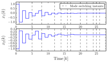
Figure 10: State trajectory versus time

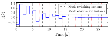
Figure 11: Control input versus time

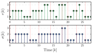
Figure 12: Actual mode $r(k)$ and sampled mode $\sigma(k)$

6 Conclusion

We proposed a feedback control framework for stabilization of switched linear stochastic systems under randomly available mode information. In this problem setting, information on the active operation mode of the switched system is assumed to be available for control purposes only at random time instants. We presented a probabilistic analysis concerning a sequence-valued stochastic process that captures the evolution of active operation mode between mode observation instants. We then used the results of this analysis to obtain sufficient almost sure asymptotic stability conditions for the zero solution of the closed-loop system.

References

- [1]
- [2] [] Bercu, B., F. Dufour and G. G. Yin (2009). ‘Almost sure stabilization for feedback controls of regime-switching linear systems with a hidden Markov chain’. IEEE Trans. Autom. Contr. 54, 2114–2125.
- [3]
- [4] [] Bernstein, D. (2009). Matrix mathematics: Theory, Facts, and Formulas. Princeton University Press: Princeton.
- [5]
- [6] [] Bolzern, P., P. Colaneri and G. De Nicolao (2004). On almost sure stability of discrete-time Markov jump linear systems. In ‘IEEE Conf. Dec. Contr.’. Nassau, Bahamas. pp. 3204–3208.
- [7]
- [8] [] Boukas, E. K. (2006). ‘Static output feedback control for stochastic hybrid systems: LMI approach’. Automatica 42, 183–188.
- [9]
- [10] [] Boyle, F. A., J. Haupt, G. L. Fudge and C. C. A. Yeh (2007). Detecting signal structure from randomly-sampled data. In ‘IEEE 14th Workshop on Stat. Sign. Proc.’. IEEE. pp. 326–330.
- [11]
- [12] [] Caines, P. E. and J. F. Zhang (1992). Adaptive control for jump parameter systems via non-linear filtering. In ‘Proc. IEEE Conf. Dec. Contr.’. Tucson, AZ. pp. 699–704.
- [13]
- [14] [] Carlen, E. and R. V. Mendes (2009). ‘Signal reconstruction by random sampling in chirp space’. Nonl. Dyn. 56(3), 223–229.
- [15]
- [16] [] Cassandras, C. G. and Lygeros, J. (Eds.) (2006). Stochastic Hybrid Systems. CRC Press. Boca Raton.
- [17]
- [18] [] Cetinkaya, A. and T. Hayakawa (2011). Stabilization of switched linear stochastic dynamical systems under limited mode information. In ‘Proc. IEEE Conf. Dec. Contr.’. Orlando, FL. pp. 8032–8037.
- [19]
- [20] [] Cetinkaya, A. and T. Hayakawa (2012). Feedback control of switched stochastic systems using uniformly sampled mode information. In ‘Proc. Amer. Contr. Conf.’. Montreal, Canada. pp. 3778–3783.
- [21]
- [22] [] Cetinkaya, A. and T. Hayakawa (2013a). Discrete-time switched stochastic control systems with randomly observed operation mode. In ‘Proc. IEEE Conf. Dec. Contr.’. Firenze, Italy. pp. 85–90.
- [23]
- [24] [] Cetinkaya, A. and T. Hayakawa (2013b). Stabilizing discrete-time switched linear stochastic systems using periodically available imprecise mode information. In ‘Proc. Amer. Contr. Conf.’. Watshington, DC, USA. pp. 3266–3271.
- [25]
- [26] [] Costa, O. L. V., M. D. Fragoso and R. P. Marques (2004). Discrete-Time Markov Jump Linear Systems. Springer.
- [27]
- [28] [] de Farias, D. P., J. C. Geromel, J. B. R. do Val and O. L. V. Costa (2000). ‘Output feedback control of Markov jump linear systems in continuous-time’. IEEE Trans. Autom. Contr. 45, 944–949.
- [29]
- [30] [] Durrett, R. (2010). Probability: Theory and Examples. Cambridge University Press: New York.
- [31]
- [32] [] Fang, Y. and K. A. Loparo (2002). ‘Stabilization of continous-time jump linear systems’. IEEE Trans. Autom. Contr. 47, 1590–1602.
- [33]
- [34] [] Geromel, J. C., A. P. C. Goncalves and A. R. Fioravanti (2009). ‘Dynamic output feedback control of discrete-time Markov jump linear systems through linear matrix inequalities’. SIAM J. Contr. Optm. 48(2), 573–593.
- [35]
- [36] [] Ghaoui, L. E. and M. A. Rami (1996). ‘Robust state-feedback stabilization of jump linear systems via LMIs’. Int. J. Robust Nonl. Contr. 6, 1015–1022.
- [37]
- [38] [] Li, C., M. Z. Q. Chen, J. Lam and X. Mao (2012). ‘On exponential almost sure stability of random jump systems’. IEEE Trans. Autom. Contr. 57(12), 3064–3077.
- [39]
- [40] [] Nassiri-Toussi, K. and P. E. Caines (1991). On the adaptive stabilization and ergodic behaviour of stochastic jump-Markov systems via nonlinear filtering. In ‘Proc. IEEE Conf. Dec. Contr.’. Brighton, England. pp. 1784–1785.
- [41]
- [42] [] Norris, J. (2009). Markov Chains. Cambridge University Press: New York.
- [43]
- [44] [] Sathanantan, S., O.Adetona, C. Beane and L. H. Keel (2008). ‘Feedback stabilization of Markov jump linear system with time-varying delay’. Stoc. Anal. App. 26, 577–594.
- [45]
- [46] [] Serfozo, R. (2009). Basics of Applied Stochastic Processes. Springer-Verlag: New York.
- [47]
- [48] [] Vargas, A. N., W. Furloni and J. B. R. do Val (2006). Constrained model predictive control of jump linear systems with noise and non-observed Markov state. In ‘Proc. Amer. Contr. Conf.’. Minneapolis, MN. pp. 929–934.
- [49]
- [50] [] Yin, G. and C. Zhu (2010). Hybrid Switching Diffusions: Properties and Applications. Springer-Verlag: New York.
- [51]