Measuring disorder in irreversible decay processes

Abstract

Rate coefficients can fluctuate in statically and dynamically disordered kinetics. Here we relate the rate coefficient for an irreversibly decaying population to the Fisher information. From this relationship we define kinetic versions of statistical-length squared and divergence that measure cumulative fluctuations in the rate coefficient. We show the difference between these kinetic quantities measures the amount of disorder, and is zero when the rate coefficient is temporally and spatially unique.

I Introduction

Rate coefficients are necessary and sufficient information in the rate laws of kinetic phenomena. To predict the average behavior of populations with these laws, it is essential to reliably estimate the rate coefficient. When fluctuations away from the average are significant in irreversible decay, predictions depend on a distribution of rate coefficients or a time varying rate coefficient Ross (2008); Plonka (2001). The terms static and dynamic disorder describe these theoretical constructs and the underlying kinetic process Zwanzig (1990). Examples of disordered kinetics include enzyme catalyzed reactions Terentyeva et al. (2012); English et al. (2005); Min et al. (2005), the dissociation of single molecules during pulling experiments Kuo et al. (2010); Chatterjee and Cherayil (2011), and hydrogen bond breaking Luzar and Chandler (1996). However, static and dynamic disorder are not mutually exclusive classifications of a process Ross (2008) or straightforward to assign a priori Dewey (1992), which raises fundamental and practical questions. How can we measure disorder from kinetic data when microscopic heterogeneity manifests in the rate coefficient? Or, when is the rate coefficient well defined? When is traditional kinetics valid?

Answering these questions requires the ability to measure disorder. An example of recent progress is an information theoretic measure of dynamic disorder Li and Komatsuzaki (2013). Such measures could enable new methods for minimizing the statistical description of rate coefficients and maximizing their predictive fidelity for data collected from simulations and experiments. In this work we demonstrate a theoretical framework for this purpose that applies to irreversible decay. Central to the theory is a measure of temporal and spatial fluctuations in the rate coefficient, when the disorder is static, dynamic, or both. Our main result is an inequality that only reduces to an equality in the absence of disorder. This result is a necessary condition for the traditional kinetics of irreversible first-order decay to be valid and the associated rate coefficients to be unique.

Consider a population of species irreversibly decaying over time. The survival probability, $S(t)$, is the probability the initial population survives up to a time $t$. This probability defines the observed or effective rate coefficient, $k(t)$, through the differential rate law

$$k(t)\equiv-\frac{d\ln S(t)}{dt},$$ (1)

characterizing the first-order decay of the entire population. If individual members of the population are experimentally indistinguishable and the overall decay of $S(t)$ is non-exponential Wang and Wolynes (1994, 1993, 1995), a disordered model for $k(t)$ may be necessary. Non-exponential decay can imply an underlying mechanism where members decay in different structural or energetic environments, or a local environment that fluctuates in time Wang and Wolynes (1995). For irreversible decay, the survival probability is the ratio of the number of members in the population at a time $t$, $N(t)$, and the number initially, $N(0)$. In terms of the effective rate coefficient it is

$$S(t)=\frac{N(t)}{N(0)}=e^{-\int_{0}^{t}{k(t^{\prime})dt^{\prime}}}.$$ (2)

Survival probabilities are the input to the theory here and a common observable; they are measurable from computer simulations and experiments. While measurements of $S(t)$ may have non-negligible statistical fluctuations, we use non-fluctuating survival probabilities to simplify the presentation of our theoretical results.

II Theory

One purpose of the theory here is to measure the fluctuations in the statistical parameter $k(t)$ for statically and dynamically disordered kinetics. For activated escape on an energy surface, measures of the fluctuations in $k(t)$ characterize the mechanism of decay over a distribution of barriers or a single barrier whose height varies in time. Our approach is to use the Fisher information, which is a natural measure of the ability to estimate statistical parameters from the probability distribution of a fluctuating observable. Colloquially, the Fisher information is the amount of “disorder” in a system or phenomenon Frieden (2004), but is it the amount of static and dynamic disorder in a kinetic process? To answer this question, a relationship between the Fisher information and rate coefficients, the parameters in kinetic phenomena, is necessary.

We relate $k(t)$ and a modified form of the Fisher information, expressed in terms of the survival probability of a decaying population through Equation 1. Assuming an exact, non-fluctuating survival probability varying smoothly over time describes the evolution of the population, a reasonable form of the Fisher information at time $t$ is

$$I(t)\equiv S(t)\left(\frac{\displaystyle d\ln S(t)}{\displaystyle dt}\right)^{2}=k(t)^{2}S(t),$$ (3)

which shows the direct relation to the effective rate coefficient. A more general form of the Fisher information may be necessary when there are statistical fluctuations in $S(t)$ Frieden (2004). Rearranging Equation 3 gives

$$k(t)=\sqrt{I(t)/S(t)}.$$ (4)

The remainder of our results stem from this connection between the Fisher information and the statistical parameter, $k(t)$, of interest in disordered kinetics.

A particularly useful aspect of the Fisher information, in general, is that it naturally defines a “statistical distance” between probability distributions. Though the notion of statistical distance was originally applied to quantum states Wootters (1981); Braunstein and Caves (1994), it is applicable to any two probability distributions. With the definition of the Fisher information above, we can measure the statistical distance between survival probabilities and relate it to the observed rate coefficient. If we take a microscopic, stochastic perspective, the rate coefficient of decay, $k(t)$, is the transition probability per unit time. In a given time interval between $t$ and $t+\delta t$, it is the ratio of the number of reacted molecules $N(0)\delta S\equiv N(0)[S(t)-S(t+\delta t)]$ and the number of unreacted molecules $N(0)S(t)$

$$k(t)\equiv\frac{\delta S}{S(t)\delta t}.$$ (5)

From this discrete form of Equation 1 and the discrete form of the relation between the time-dependent rate coefficient and the Fisher information in Equation 4, we define a dimensionless statistical distance

$$\delta s^{2}\equiv k(t)^{2}\delta t^{2}=\frac{I(t)}{S(t)}\delta t^{2}=\left[\frac{\delta S}{S(t)}\right]^{2}=\left[\delta\ln S\right]^{2}$$ (6)

between the logarithm of the survival probabilities at $t$ and $t+\delta t$. If the fractional change in the population from one time to the next, $\delta S/S(t)$, is a fixed value, the rate coefficient is independent of time and the distance between $\ln S(t)$ and $\ln S(t+\delta t)$ is constant. We can interpret the statistical distance as a criterion for the distinguishability of $\ln S(t)$ at two times, since it is zero if the survival probability is time independent, or as the square of the transition probability $k(t)\delta t$ during $\delta t$.

During an irreversible decay process from an initial time $t_{i}$ to a final time $t_{f}$, and letting $\delta t\to 0$, we can integrate the arc length of the logarithmic survival curve $\ln S(t)$

$$\mathcal{L}(\Delta t)=\int_{t_{i}}^{t_{f}}ds=\int_{t_{i}}^{t_{f}}\sqrt{\frac{I(t)}{S(t)}}\,dt=\int_{t_{i}}^{t_{f}}k(t)\,dt$$ (7)

to get the statistical length, $-\ln S(t)\big{|}_{S(t_{i})}^{S(t_{f})}$, measuring the cumulative rate coefficient. The statistical length is infinite for an infinite time interval $\Delta t=t_{f}-t_{i}$. Another useful quantity, related to the statistical length, is the Fisher divergence, $\mathcal{J}(\Delta t)$. The Fisher divergence we define as

$$\frac{\mathcal{J}(\Delta t)}{\Delta t}=\int_{t_{i}}^{t_{f}}ds^{2}=\int_{t_{i}}^{t_{f}}\frac{I(t)}{S(t)}\,dt=\int_{t_{i}}^{t_{f}}k(t)^{2}\,dt,$$ (8)

the time integrated square of the rate coefficient (times the magnitude of the time interval). Both the statistical length and the Fisher divergence are cumulative properties of the rate coefficient, identified through Equation 4 for irreversibly decaying populations. These properties for the history of $k(t)$ satisfy an inequality

$$\mathcal{L}(\Delta t)^{2}\leq\mathcal{J}(\Delta t),$$ (9)

which is our main result. An analogous inequality in finite-time thermodynamics is a bound on the dissipation in an irreversible process Salamon and Berry (1983); Salamon, Nulton, and Berry (1985); Feldmann et al. (1985); Crooks (2007); Feng and Crooks (2009); Sivak and Crooks (2012).

We will show the inequality above measures disorder in kinetic phenomena and is an equality in the absence of both static or dynamic disorder. Some evidence for this comes from the inequality $\mathcal{J}(\Delta t)-\mathcal{L}(\Delta t)^{2}\geq 0$ in terms of the observed rate coefficient

$$\Delta t\int_{t_{i}}^{t_{f}}k(t)^{2}\,dt-\left[\int_{t_{i}}^{t_{f}}k(t)\,dt\right]^{2} \geq 0.$$ (10)

For decay processes with a time independent rate coefficient, there is no disorder, and the bound holds $\left(k\Delta t\right)^{2}=k^{2}\Delta t^{2}$. While this finding is suggestive, we can show more concretely that the inequality measures the variation of the rate coefficient in irreversible decay kinetics. We turn to this now and show the inequality measures the amount of disorder during a given time interval. As a proof-of-principle we apply the theory to widely used kinetic models for populations decaying non-exponentially. Note, however, that the theory is model independent.

III Kinetic model with dynamic disorder

To demonstrate the inequality measures dynamic disorder, we consider the Kohlrausch-Williams-Watts (KWW) stretched exponential survival function. This empirical model is a widely used phenomenological description of relaxation in complex media. It has been applied to the discharge of capacitors Kohlrausch (1854), the dielectric spectra of polymers Williams and Watts (1970), and more recently the fluorescence of single molecules Flomenbom et al. (2005). The survival probability, $\exp\left[-(\omega t)^{\beta}\right]$, has two adjustable parameters $\omega$ - a characteristic, time-independent rate coefficient or inverse time scale - and $0<\beta\leq 1$ measuring the “cooperativity” of decay events - being nearer or equal to $1$ for independent decay events and nearer $0$ for coupled decay events (Figure 1). Fitting data to this function when the decay is non-exponential implicitly assumes the kinetics are dynamically disordered.

Figure 1(a) shows analytical results for how the natural logarithm of the survival function versus time depends on the value of $\beta$. There is a linear dependence on time only when $\beta=1$, corresponding to exponential kinetics and a time independent rate coefficient $k(t)\to\omega$. For all other $\beta$ values the survival function decays faster than exponential before, and slower than exponential after, $t=1/\omega=1$. These stretched exponential decays have a time-dependent rate coefficient $k(t)=\beta\left(\omega t\right)^{\beta}/t$ when $\beta\neq 1$ from Figure 1(b). The effective rate coefficient is the (negative of the) slope of the graph of $\ln S(t)$ versus $t$. Through the rate law, the decrease in $k(t)$ over time indicates a decrease in the rate of decay; this also means the number of species decaying in a unit time interval is decreasing. Furthermore, if we interpret the decay as an activated process over an energy barrier Zwanzig (1990), a decrease in $k(t)$ implies an increase in barrier height and slowing rate of escape. In the limit of long times, the rate coefficient $k(t)$ is effectively constant, regardless of $\beta$. The value of $\beta$ determines the rate at which $k(t)$ reaches this limit: smaller $\beta$ values lead to a more rapid decline of $k(t)$.

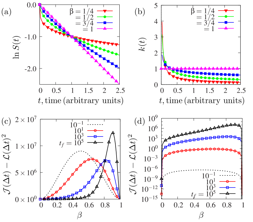
Figure 1: (Color online)(a) Logarithmic Kohlrausch-Williams-Watts survival curves $\ln S(t)$ for stretched exponential decay with $\omega=1$ and $\beta=\tfrac{1}{4}$, $\tfrac{1}{2}$, $\tfrac{3}{4}$, and exponential decay $\beta=1$. (b) The rate of decay of the observed rate coefficient $k(t)$ over time depends on $\beta$, $0<\beta\leq 1$. (c) $\mathcal{J}(\Delta t)-\mathcal{L}(\Delta t)^{2}\geq 0$ over the range of $\beta$ values for the final times of $t_{f}=10^{-1}$, $10^{1}$, $10^{3}$, $10^{5}$ and an initial time of $t_{i}=1$, in arbitrary time units. The difference is scaled by an arbitrary factor of $2\times 10^{13}$, $10^{7}$, $2\times 10^{3}$, and $1$ for a direct comparison. (d) $\mathcal{J}(\Delta t)-\mathcal{L}(\Delta t)^{2}$ versus the disorder parameter $\beta$ on a logarithmic scale. $\mathcal{J}(\Delta t)=\mathcal{L}(\Delta t)^{2}$ for all $\beta$ and any time interval when there is no dynamic disorder – when $\beta=1$ and $k=\omega$.

From the effective rate coefficient, we find the statistical length $\mathcal{L}_{\textrm{KWW}}(\Delta t)=\omega^{\beta}t^{\beta}\big{|}_{t_{i}}^{t_{f}}$ and, for $\beta\neq\tfrac{1}{2}$, the divergence

$$\mathcal{J}_{\textrm{KWW}}(\Delta t)=\frac{\beta^{2}}{2\beta-1}\omega^{2\beta}\Delta t\,t^{2\beta-1}\big{|}_{t_{i}}^{t_{f}}.$$ (11)

For $\beta=\tfrac{1}{2}$, the divergence is $\beta^{2}\omega^{2\beta}\Delta t\ln t\big{|}_{t_{i}}^{t_{f}}$. From these results for stretched exponential kinetics of the KWW type, we find $\mathcal{J}(\Delta t)\geq\mathcal{L}(\Delta t)^{2}$ (dropping the subscript KWW for clarity) and can show the inequality measures the amount of dynamic disorder associated with the empirical parameter $\beta$.

The temporal variation of $k(t)$ on the observational time scale dictates the magnitude of $\mathcal{J}(\Delta t)-\mathcal{L}(\Delta t)^{2}$. Since $\beta$ determines how strongly $k(t)$ varies in time, we show $\mathcal{J}(\Delta t)-\mathcal{L}(\Delta t)^{2}$ over the range of $\beta$ for select final times in Figure 1(c) and (d). The plots are at four different final times $t_{f}=10^{-1}$, $10$, $10^{3}$, $10^{5}$ and an initial time $t_{i}=1$ in arbitrary units. Most striking in Figure 1(c) and (d), is the maximum in $\mathcal{J}(\Delta t)-\mathcal{L}(\Delta t)^{2}$. We see the maximum of the inequality is at a $\beta$ greater than or equal to $0.5$ for all non-zero time intervals and all $t_{f}$. At final times less than $1/\omega$, the difference is symmetric with a maximum at $\beta=0.5$. With increasing $t_{f}$, the curve becomes asymmetric and the maximum shifts to higher $\beta$ values.

In part, the maximum comes from $\mathcal{J}(\Delta t)-\mathcal{L}(\Delta t)^{2}$ being zero at the limiting values of $\beta$ where the effective rate coefficient is time-independent. When $\beta=1$, the decay is exponential, $k(t)=\omega$, and $\mathcal{J}(\Delta t)=\mathcal{L}(\Delta t)^{2}$ for all final and initial times $t_{f}>t_{i}$. The effective rate coefficient is also zero when $\beta=0$, though this limit is typically excluded from the KWW model; however, when the rate coefficient is zero the equality again holds. Since $\mathcal{J}(\Delta t)-\mathcal{L}(\Delta t)^{2}$ must be zero at the limits of the $\beta$ range, and is non-zero between these limits, there must be a maximum at intermediate $\beta$ values. In this case, and the model we discuss next, there is a single maximum in $\mathcal{J}(\Delta t)-\mathcal{L}(\Delta t)^{2}$ versus $\beta$. A single maximum results when the decay is monotonic, and non-exponential, with a time-varying rate coefficient between two limits where the rate coefficient is constant. However, if the decay is more complex, or if the kinetics are driven, more maxima are possible.

The maximum in $\mathcal{J}(\Delta t)-\mathcal{L}(\Delta t)^{2}$ shown in Figure 1(c) and (d) is also the result of how the history of $k(t)$ depends on $\beta$ in this model. Panel (b) shows that decreasing $\beta$ also increases the difference between $k(t_{f})$ and $k(t_{i})$, which would imply an increase in the difference between the barrier heights at $t_{f}$ and $t_{i}$ for an activated process. As $\beta$ decreases from one to zero, this increase in the variation of the rate coefficient initially leads to a greater inequality between $\mathcal{J}(\Delta t)$ and $\mathcal{L}(\Delta t)^{2}$. However, as $\beta$ continues to decrease, the effective rate coefficient also becomes a more rapidly decreasing function of time (Figure 1(b)). Consequently, significant changes in the magnitude of $k(t)$ can become relatively small portions of the observational time window. For example, at $t_{f}=10^{5}$ the effective rate coefficient varies little over the majority of the observation time for $\beta<0.5$, and $\mathcal{J}(\Delta t)\approx\mathcal{L}(\Delta t)^{2}$. But, for $\beta>0.5$, $k(t)$ is more strongly dependent on time over the interval $t_{f}-t_{i}$ and $\mathcal{J}(\Delta t)>\mathcal{L}(\Delta t)^{2}$. Overall, the magnitude of the $\mathcal{J}(\Delta t)-\mathcal{L}(\Delta t)^{2}$ reflects the both the variation of $k(t)$ in time and the fraction of the observation time where those changes occur. The maximum in the inequality versus $\beta$ reflects the competition of these factors.

IV Kinetic model with static disorder

The difference between $\mathcal{J}(\Delta t)$ and $\mathcal{L}^{2}(\Delta t)$ also measures the amount of static disorder in irreversible decay kinetics over a time interval. As a tractable example, consider the model with two experimentally indistinguishable states, $A$ and $A^{\prime}$ Goldanskii, Kozhushner, and Trakhtenberg (1997).

These states might be the internal configurations of a reactive molecule that can interconvert through isomerization or two energy levels leading to unimolecular dissociation in the gas phase. The states are in equilibrium and so a population occupying these states will undergo transitions between them. A population occupying the $A$ and $A^{\prime}$ states can also decay irreversibly to $B$ with rates characterized by two time-independent rate coefficients, $\omega$ and $\omega^{\prime}$. If the individual decay out of $A$ and $A^{\prime}$ have different characteristic rates, it may be necessary to characterize the collective decay from the $A$ states with both rate coefficients. Since only two rate coefficients $\omega$ and $\omega^{\prime}$ represent the “fluctuations” in the rate coefficient, this is the simplest case of potentially statically disordered kinetics (Figure 2), and is readily generalizable to a continuum of $A$ states.

The phenomenological rate equations are

$$\frac{\displaystyle dN_{A}}{\displaystyle dt} = -(\omega+\lambda)N_{A}+a\lambda N_{A^{\prime}}$$

$$\frac{\displaystyle dN_{A^{\prime}}}{\displaystyle dt} = -(\omega^{\prime}+a\lambda)N_{A^{\prime}}+\lambda N_{A}$$

for the number of species in state $A$, $N_{A}$, and $A^{\prime}$, $N_{A^{\prime}}$. These numbers are exact and not fluctuating in time. Whether the decay from $A$ and $A^{\prime}$ is exponential or non-exponential depends on the relative rates of interconversion and reaction. Two limiting solutions to these rate equations are of particular interest Plonka (2001). Each limit affects the analytical form of the survival probability for the population of the $A$ and $A^{\prime}$ states

$$S(t)=\frac{N_{A}(t)+N_{A^{\prime}}(t)}{N_{A}(0)+N_{A^{\prime}}(0)}.$$ (12)

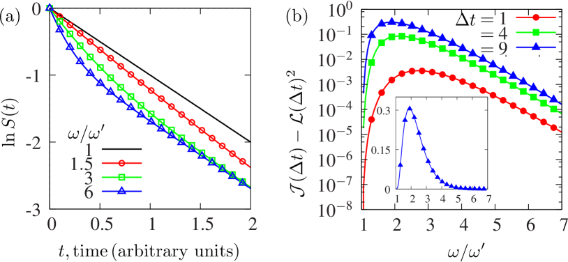
Figure 2: (Color online)(a) Logarithmic survival plot for the kinetic scheme in the text for $a=1$ and $\omega^{\prime}=1$. The decay kinetics are statically disordered when $\omega\neq\omega^{\prime}$, leading to the non-exponential relaxation of $S(t)$ and the non-linearity of $\ln S(t)$ in time. The kinetics are exponential when $\omega=\omega^{\prime}$ and $\ln S(t)$ versus $t$ is linear (black line). There is no disorder when $\omega\neq\omega^{\prime}$ at long times when the slower channel dominates decay. (b) The graph of $\mathcal{J}(\Delta t)-\mathcal{L}(\Delta t)^{2}$ reflects these facts, showing this difference measures the amount of static disorder over a range of relative decay rates $\omega/\omega^{\prime}$ ($\omega^{\prime}=1$) and time intervals $\Delta t=1$, $4$, and $9$ on a logarithmic scale. The inset is on a linear scale for $\Delta t=9$. $\mathcal{J}(\Delta t)-\mathcal{L}(\Delta t)^{2}$ is zero if decay is exponential (when $\omega=\omega^{\prime}$ or when $\omega\gg\omega^{\prime}$), but nonzero otherwise.

First, in the limit where interconversion between $A$ and $A^{\prime}$ is fast compared to the reaction, $\lambda\to\infty\gg\omega,\omega^{\prime}$, the survival probability is

$$S(t)\sim\exp{\left[-\left(\frac{a}{1+a}\omega+\frac{1}{1+a}\omega^{\prime}\right)t\right]}.$$ (13)

and the population decays exponentially. From Equation 1, the observed rate coefficient $k(t)$ is time independent and a weighted-average of $\omega$ and $\omega^{\prime}$, $\tfrac{a}{1+a}\omega+\tfrac{1}{1+a}\omega^{\prime}$. From this limiting survival probability it follows that the divergence and length squared are equal, $\mathcal{L}^{2}(\Delta t)=\mathcal{J}(\Delta t)=k(t)^{2}\Delta t^{2}$. This result illustrates that to satisfy the bound, the $A$ states must be kinetically indistinguishable, which happens here because the population collectively decays to products from one effective state.

Second, in the limit $\lambda\to 0$, the transitions between the $A$ states are slow relative to those of reaction. When the decay from $A$ and $A^{\prime}$ is independent, the net decay is bi-exponential

$$S(t)\sim\frac{a}{1+a}e^{-\omega t}+\frac{1}{1+a}e^{-\omega^{\prime}t}.$$ (14)

The logarithmic dependence of this survival function versus time in Figure 2(a) is linear, and the decay of $S(t)$ is effectively exponential, if the decay from the $A$ and $A^{\prime}$ states have the same rate coefficients $\omega=\omega^{\prime}$. In this case, we again find $\mathcal{L}^{2}(\Delta t)=\mathcal{J}(\Delta t)$. However, this condition breaks when the kinetics are statically disordered $\omega\neq\omega^{\prime}$ and decay from $A$ and $A^{\prime}$ competitively depletes the population, leading to the non-exponential decay in Figure 2(a). The $S(t)$ in this regime causes the observed rate coefficient $k(t)$ to vary in time. Only when there is static disorder in this model does $\mathcal{L}(\Delta t)^{2}$ not equal $\mathcal{J}(\Delta t)$.

The relative magnitude of $\omega$ and $\omega^{\prime}$, which we measure with the ratio $\omega/\omega^{\prime}$, and the time interval, $\Delta t$, control the degree of static disorder. The difference $\mathcal{J}(\Delta t)-\mathcal{L}(\Delta t)^{2}$ is sensitive to both of these factors. Figure 2(b) illustrates the dependence of the inequality on $\omega/\omega^{\prime}$ and assumes the survival function is valid, $\omega,\omega^{\prime}\ll\lambda$, over the range of interest. Varying $\omega/\omega^{\prime}$ shows the difference between the divergence and length squared is positive, has a maximum that depends on the time interval, and tends to zero with increasing $\omega/\omega^{\prime}$. In the figure, the difference is shown for three final times $t_{f}=2$, $5$, and $10$ and $t_{i}=1$, in arbitrary units. A logarithmic scale allows direct comparison of these curves (the vertical axis in the inset has a linear scale).

An inequality between $\mathcal{L}(\Delta t)^{2}$ and $\mathcal{J}(\Delta t)$ gives quantitative insight into the mechanism of kinetic processes, when only the survival of the entire population is available. From Figure 2(b) the inequality grows but as the disparity in the rate coefficients of each decay path increases further, there becomes a separation of timescales, one path decays on times that are increasingly short in comparison to the time interval of interest. Just as for the KWW model, there is a maximum in the inequality between the divergence and length squared. In the limit $\omega\gg\omega^{\prime}$, $\mathcal{J}(\Delta t)=\mathcal{L}(\Delta t)^{2}$, indicating exponential decay and a single characteristic rate coefficient. The maximum is understandable from the survival function: with increasing $\omega$ or $t$, the term $e^{-\omega t}$ decreases until, ultimately, the decay channel contributes negligibly to the overall decay of the population – the kinetics are exponential with the characteristic rate of the slower decay channel, $k(t)\to\omega^{\prime}=1$. The survival function in Equation 14 becomes $S(t)\sim(1+a)^{-1}\exp{(-\omega^{\prime}t)}$.

Together these findings demonstrate the inequality is a statement about whether a single rate coefficient is sufficient for irreversible rate processes. The rate coefficient is a unique constant only when $\mathcal{J}(\Delta t)=\mathcal{L}(\Delta t)^{2}$, and the decaying states are kinetically indistinguishable. Otherwise, the inequality between $\mathcal{J}(\Delta t)$ and $\mathcal{L}(\Delta t)^{2}$ measures the dispersion in the rate coefficient–though it does not distinguish between statically and dynamically disordered kinetics. The inequality both results from, and measures, the heterogeneity of microscopic environments that ultimately produce disordered kinetics. For activated processes over an energy barrier, heterogeneous environments can cause either fluctuating barrier heights or a distribution of barriers through steric/energetic effects. Consequently, the inequality could be used to investigate the local structure around reaction sites in disordered media and the dependence of rate processes on energetic or structural effects of the environment Siebrand and Wildman (1986). The equality signifies when the interconversion between decaying states is faster than decay, when there is no microscopic heterogeneity to cause a distribution of rate coefficients, and when observations of the process are on a time scale where fast decay processes are insignificant to the longer term survival of the population. Under these circumstances traditional kinetics holds.

V Conclusions

In summary, the inequality between $\mathcal{L}^{2}(\Delta t)$ and $\mathcal{J}(\Delta t)$ measures the amount of static and dynamic disorder in irreversible decay kinetics. The inequality follows from the relation between the rate coefficient for decay and the Fisher information. It relies on two functions of the Fisher information - a statistical length and the Fisher divergence for the decaying population - which are properties of the history of fluctuations in the rate coefficient. This relationship is a quantitative signature of when decay kinetics are accurately described by a fluctuating rate coefficient (measured by the inequality) and when a single, unique rate constant is sufficient. Traditional kinetics corresponds to the condition $\mathcal{L}^{2}(\Delta t)=\mathcal{J}(\Delta t)$. Our results suggest minimizing the difference between $\mathcal{L}^{2}(\Delta t)$ and $\mathcal{J}(\Delta t)$, when it is desirable to minimize the statistical description of kinetic phenomena with rate coefficients or to maximize the predictive fidelity of rate coefficients extracted from experimental or simulation data. In the future, this framework may also be useful in the analysis of, potentially complex, chemical reactions with fluctuating rates.

VI Acknowledgements

This work was supported as part of the Non-Equilibrium Energy Research Center (NERC), an Energy Frontier Research Center funded by the U.S. Department of Energy, Office of Science, Basic Energy Sciences under Award #DE-SC0000989. This material is based upon work supported in part by the U.S. Army Research Laboratory and the U.S. Army Research Office under grant number W911NF-14-1-0359.

References

- Ross (2008) J. Ross, Thermodynamics and Fluctuations far from Equilibrium (Springer, 2008).
- Plonka (2001) A. Plonka, Dispersive Kinetics (Springer, 2001).
- Zwanzig (1990) R. Zwanzig, Acc. Chem. Res. 23, 148 (1990).
- Terentyeva et al. (2012) T. G. Terentyeva, H. Engelkamp, A. E. Rowan, T. Komatsuzaki, J. Hofkens, C.-B. Li, and K. Blank, ACS Nano 6, 346 (2012).
- English et al. (2005) B. P. English, W. Min, A. M. V. Oijen, K. T. Lee, G. Luo, H. Sun, B. J. Cherayil, S. C. Kou, and S. X. Xie, Nat. Chem. Biol. 2, 87 (2005).
- Min et al. (2005) W. Min, B. P. English, G. Luo, B. J. Cherayil, S. C. Kuo, and X. S. Xie, Acc. Chem. Res. 38, 923 (2005).
- Kuo et al. (2010) T.-L. Kuo, S. Garcia-Manyes, J. Li, I. Barel, H. Lu, B. J. Berne, M. Urbakh, J. Klafter, and J. M. Fernández, Proc. Natl. Acad. Sci. U.S.A. 107, 11336 (2010).
- Chatterjee and Cherayil (2011) D. Chatterjee and B. J. Cherayil, J. Chem. Phys. 134, 165104 (2011).
- Luzar and Chandler (1996) A. Luzar and D. Chandler, Phys. Rev. Lett. 76, 928 (1996).
- Dewey (1992) T. G. Dewey, Chem. Phys. 161, 339 (1992).
- Li and Komatsuzaki (2013) C.-B. Li and T. Komatsuzaki, Phys. Rev. Lett. 111, 058301 (2013).
- Wang and Wolynes (1994) J. Wang and P. G. Wolynes, Chem. Phys. 180, 141 (1994).
- Wang and Wolynes (1993) J. Wang and P. G. Wolynes, Chem. Phys. Lett. 212, 427 (1993).
- Wang and Wolynes (1995) J. Wang and P. Wolynes, Phys. Rev. Lett. 74, 4317 (1995).
- Frieden (2004) B. R. Frieden, Science from Fisher Information: A Unification, 2nd ed. (Cambridge University Press, 2004).
- Wootters (1981) W. K. Wootters, Phys. Rev. D 23, 357 (1981).
- Braunstein and Caves (1994) S. L. Braunstein and C. M. Caves, Phys. Rev. Lett. 72, 3439 (1994).
- Salamon and Berry (1983) P. Salamon and R. S. Berry, Phys. Rev. Lett. 51, 1127 (1983).
- Salamon, Nulton, and Berry (1985) P. Salamon, J. D. Nulton, and R. S. Berry, J. Chem. Phys. 82, 2433 (1985).
- Feldmann et al. (1985) T. Feldmann, B. Andresen, A. Qi, and P. Salamon, J. Chem. Phys. 83, 5849 (1985).
- Crooks (2007) G. E. Crooks, Phys. Rev. Lett. 99, 100602 (2007).
- Feng and Crooks (2009) E. H. Feng and G. E. Crooks, Phys. Rev. E 79, 012104 (2009).
- Sivak and Crooks (2012) D. A. Sivak and G. E. Crooks, Phys. Rev. Lett. 108, 190602 (2012).
- Kohlrausch (1854) R. Kohlrausch, Annalen der Physik 167, 56 (1854).
- Williams and Watts (1970) G. Williams and D. C. Watts, Trans. Faraday Soc. 66, 80 (1970).
- Flomenbom et al. (2005) O. Flomenbom, K. Velonia, D. Loos, S. Masuo, M. Cotlet, Y. Engelborghs, J. Hofkens, A. E. Rowan, R. J. M. Nolte, M. Van der Auweraer, F. C. de Schryver, and J. Klafter, Proc. Natl. Acad. Sci. U.S.A. 102, 2368 (2005).
- Goldanskii, Kozhushner, and Trakhtenberg (1997) V. I. Goldanskii, M. A. Kozhushner, and L. I. Trakhtenberg, J. Phys. Chem. B 101, 10024 (1997).
- Siebrand and Wildman (1986) W. Siebrand and T. A. Wildman, Acc. Chem. Res. 19, 238 (1986).