Spectral networks and higher web-like structures

We derive traffic rule for spectral networks for $A_{2}$ theory for Riemann surface $C$ with punctures and use it to study in details the moduli space $\mathcal{M}$ of flat $GL(3,\mathbb{C})$ connections on $\mathbb{P}^{1}$ with 3 full punctures. We apply the simplified traffic rule to find the global description of $\mathcal{M}$ as the fibration with symplectic fibers and to study the space of line defects in 4d theory corresponding to the conformal point in the base of $\mathcal{M}.$ We define higher web-like structures, not previously discussed in the literature. They give rise to line defects independent of the defects corresponding to the traces of holonomies.

1 Introduction

Moduli spaces of flat $GL(K,\mathbb{C})$ connections on Riemann surfaces with punctures play a key role [1, 2] in the study of line defects in $\mathcal{N}=2,d=4$ supersymmetric theories. In particular, the algebra of functions on these moduli spaces is relevant for computing the Operator Product Expansion of line defects.

An explicit description of moduli spaces of flat $GL(K,\mathbb{C})$ connections and their algebras of functions was proposed in [3, 4] by means of spectral networks. Alternatively, Fock-Goncharov construction [8] of moduli spaces of flat $PGL(K,\mathbb{C})$ connections was fruitfully used [9, 10] in the literature on line defects. Traffic rule is a crucial tool in the description of these moduli spaces. For $A_{1}$ theory the traffic rule was formulated in [5, 6] and used in [1, 4]. See also a review [7] on this subject. In this note we derive traffic rule for $A_{2}$ theory for general Riemann surface $C$(without boundary but with punctures) and use it to discuss in details the moduli space $\mathcal{M}$ of flat $GL(3,\mathbb{C})$ connections on $\mathbb{P}^{1}$ with 3 full punctures.

In the spectral network approach, one triangulates a Riemann surface $C$ such that punctures serve as vertices of the triangles and considers branched cover $\Sigma$ with ${\frac{1}{2}}K(K-1)$ branch points in each triangle. To explicitly write down a monodromy of a flat $GL(K,\mathbb{C})$ connection on $C$ around an arbitrary contour one needs to formulate the traffic rule. For $A_{K}$ theory with $K>1$ the prescription of how to cross branch cuts and edges of the triangles was missing, and we provide it in Section 3 for $A_{2}$ theory. Then we pass to a simplified version of spectral network which is sufficient to describe monodromies of homotopy classes of curves. Traffic rule for simplified spectral networks generalizes easily to $A_{K}$ theory with $K>2$ (see Section 4).

We apply the simplified traffic rule to find the global description of $\mathcal{M}$ as the fibration with symplectic fibers given in (11) and to study the space of line defects in 4d theory corresponding to the conformal point in the base of $\mathcal{M}.$ We show that basic webs give rise to line defects that are linear combinations of defects arising from traces of holonomies. We define higher web-like structures, not previously discussed in the literature, and show that they give rise to line defects independent of the defects corresponding to the traces of holonomies.

This note is organized as follows. In Section 2 we review some basic facts about the moduli space $\mathcal{M}$ of flat $GL(3,\mathbb{C})$ connections on $C=\mathbb{P}^{1}/\{v_{1},v_{2},v_{3}\}.$ In Section 3 we provide traffic rule for $A_{2}$ theory for general $C$ (without boundary but with punctures) and use the traffic rule to describe $\mathcal{M}$ by means of spectral networks and to find the global description of $\mathcal{M}.$ In Section 4 we formulate the simplified traffic rule for $A_{2}$ theory and generalize it for $A_{K}$ theory with $K>2.$ In Section 5 we discuss the space of line defects at the conformal point. In Section 6 we give an explicit relation between the spectral network and Fock-Goncharov descriptions.

2 Flat $GL(3,\mathbb{C})$ connections on $\mathbb{P}^{1}$ with three punctures

Moduli space $\mathcal{M}$ of flat $GL(3,\mathbb{C})$ connections on $C=\mathbb{P}^{1}/\{v_{1},v_{2},v_{3}\}$ can be parametrized by three $GL(3,\mathbb{C})$ matrices $M_{1},M_{2},M_{3}$ up to simultaneous conjugation $M_{i}\mapsto hM_{i}h^{-1}$ and a constraint

$$M_{1}M_{2}M_{3}={\mathbb{I}}.$$

These matrices are monodromies around the punctures with some fixed based point. Counting independent parameters gives ten-dimensional moduli space:

$$3\times 9-9-8=10$$

where we took into account that conjugation with $h=\lambda{\mathbb{I}}$ lives the constraint invariant.

$\mathcal{M}$ is a Poisson manifold and the Darboux coordinates $X_{\gamma_{i}}$can be identified, following the general proposal in [3], with holonomies of a flat abelian connection around basic non-trivial 1-cycles $\gamma_{i}$ on $3:1$ branched cover $\Sigma\mapsto C.$ There are three branch points of the type 12, 23,12 respectively in each triangle of a chosen triangulation of $C.$ The Poisson structure is simply

$$\{X_{\gamma_{i}},X_{\gamma_{j}}\}=\langle\gamma_{i},\gamma_{j}\rangle X_{\gamma_{i}}\,X_{\gamma_{j}}$$

where $\langle\cdot,\cdot\rangle$ is the intersection pairing between the 1-cycles. Applying Hurwitz formula, we find that for $C=\mathbb{P}^{1}/\{v_{1},v_{2},v_{3}\}$ the cover $\Sigma$ is $\mathbb{T}^{2}$ with nine punctures. The basis of 1-cycles on $\Sigma$ is shown in Figure 1.

Figure 1: Basis of non-trivial 1-cycles on $\Sigma$. Numbers indicate sheets of the cover.

The only non-zero Poisson bracket is

$$\{X_{\alpha},X_{\beta}\}=X_{\alpha}\,X_{\beta}$$

The 1-cycles $\gamma^{(a)}_{k}$ go around nine punctures $p^{(a)}_{k}$ on $\Sigma$ which are lifts to the $k=1,2,3$ sheet of the three punctures $v_{a}$ on $C$. The corresponding Darboux coordinates $X_{\gamma^{(a)}_{k}}$ are in the center of the Poisson algebra and satisfy

$$\prod_{a=1}^{3}\prod_{k=1}^{3}X_{\gamma^{(a)}_{k}}=1.$$

$\mathcal{M}$ has the structure of a fibration over the manifold parametrized by $X_{\gamma^{(a)}_{k}}$ with a fiber being a complex symplectic manifold with coordinates $X_{\alpha},X_{\beta}.$ By fixing conjugacy classes of monodromies around punctures, one fixes a point in the base and works with this symplectic manifold.

3 $\mathcal{M}$ from spectral network

Here we describe $\mathcal{M}$ by means of spectral networks. In Section 3.1 we discuss the details of the traffic rule required to construct a flat connection on a trivialized $GL(3,\mathbb{C})$ bundle on a Riemann surface $C$ with punctures. In Section 3.2 we apply this to compute monodromies around punctures for $C=\mathbb{P}^{1}/\{v_{1},v_{2},v_{3}\}$ and to provide the global description of $\mathcal{M}.$

3.1 Traffic rule for $A_{2}$ theory

The notion of a spectral network was introduced in [3] as a tool for the computation of BPS degeneracies in $\mathcal{N}=2$ theories. In the same paper, it was also proposed to use spectral networks to construct flat connections on a trivialized $GL(K,\mathbb{C})$ bundle on a Riemann surface $C$ with punctures. In this construction, one triangulates $C$ such that punctures serve as vertices of the triangles and considers branched cover $\Sigma$ with ${\frac{1}{2}}K(K-1)$ branch points in each triangle. $S$-walls of various type start at branch points and go to the punctures in such a way that in each triangle there is a level K lift of $AD_{1}$ theory. In [4] two types of level K lifts were introduced - Yin and Yang. In Section 3 we work with the Yin type, but in Section 4 we describe simplified traffic rule for both types. Given a triangulation of $C$ and a trivialization of the $GL(K,\mathbb{C})$ bundle, an assignment of Yin and Yang networks to the triangles gives a chart of an atlas with which we can describe $\mathcal{M}.$

$GL(K,\mathbb{C})$ matrices that describe crossing S-walls (from right to left) were found in [4]. For example for $K=3,$ these matrices are

$$S_{12}=\begin{pmatrix}1&1&0\cr 0&1&0\cr 0&0&1\end{pmatrix},\quad S_{23}(r)=\begin{pmatrix}r&0&0\cr 0&1&1\cr 0&0&1\end{pmatrix},\quad S_{21}(r)=\begin{pmatrix}1&0&0\cr-1&1&0\cr 0&0&r\end{pmatrix},\quad S_{32}=\begin{pmatrix}1&0&0\cr 0&1&0\cr 0&-1&1\end{pmatrix}.$$

Here $r$ is a complex parameter for each triangle.

To explicitly write down a monodromy of a flat connection on a trivialized $GL(K,\mathbb{C})$ bundle on $C$ around an arbitrary contour $\mathcal{P}$ one needs to formulate the traffic rule i.e. prescribe what $GL(K,\mathbb{C})$ transformation corresponds to crossing of the path $\mathcal{P}$ with $S$-walls as well as with various branch cuts and edges of the triangles. For $A_{1}$ theory the complete traffic rule was formulated in [1, 4]. For $A_{K}$ theory with $K>1$ the prescription of how to cross branch cuts and edges was missing, and we provide it in this note.

It is nontrivial to observe that the traffic rule depends on a choice of branch cuts. Moreover, each branch cut is split into segments by $S$-walls intersecting it. To ensure the flatness of the connection, implying that monodromy is an identity matrix around any contractible cycle on $C,$ we have to assign certain matrices $\sigma_{I}$ to crossing various segments $I$ of the branch cuts. It is sufficient to determine $\sigma_{I}$ for $C=\mathbb{P}^{1}/\{v_{1},v_{2},v_{3}\}$ (as in Figure 2) since similar matrices, though depending on the parameter $r$ for the appropriate triangle, describe crossing the branch cuts in the other triangles for more general $C$ (see Figure 3).

For technical reasons we choose branch cuts so that each edge is either not intersected by branch cuts or is intersected precisely by ${\frac{1}{2}}K(K-1)$ branch cuts. If the edge of the triangle is not intersected by branch cuts, we assign diagonal matrix to the crossing of this edge. If the edge $j$ is crossed by the cuts, we assign diagonal crossing matrix $D_{(j;1)}$ to the left-most segment of the edge, while crossing matrices $D_{(j;a)}$ for all other segments of this edge (i.e. $a=2,\ldots,{\frac{1}{2}}K(K-1)+1$ ) are determined in terms of $D_{(j;1)}$ and matrices $\sigma_{I}$ of crossing the branch cuts. It turns out that $D_{(j;a)}\,a=2,\ldots,{\frac{1}{2}}K(K-1)$ are non-diagonal matrices.

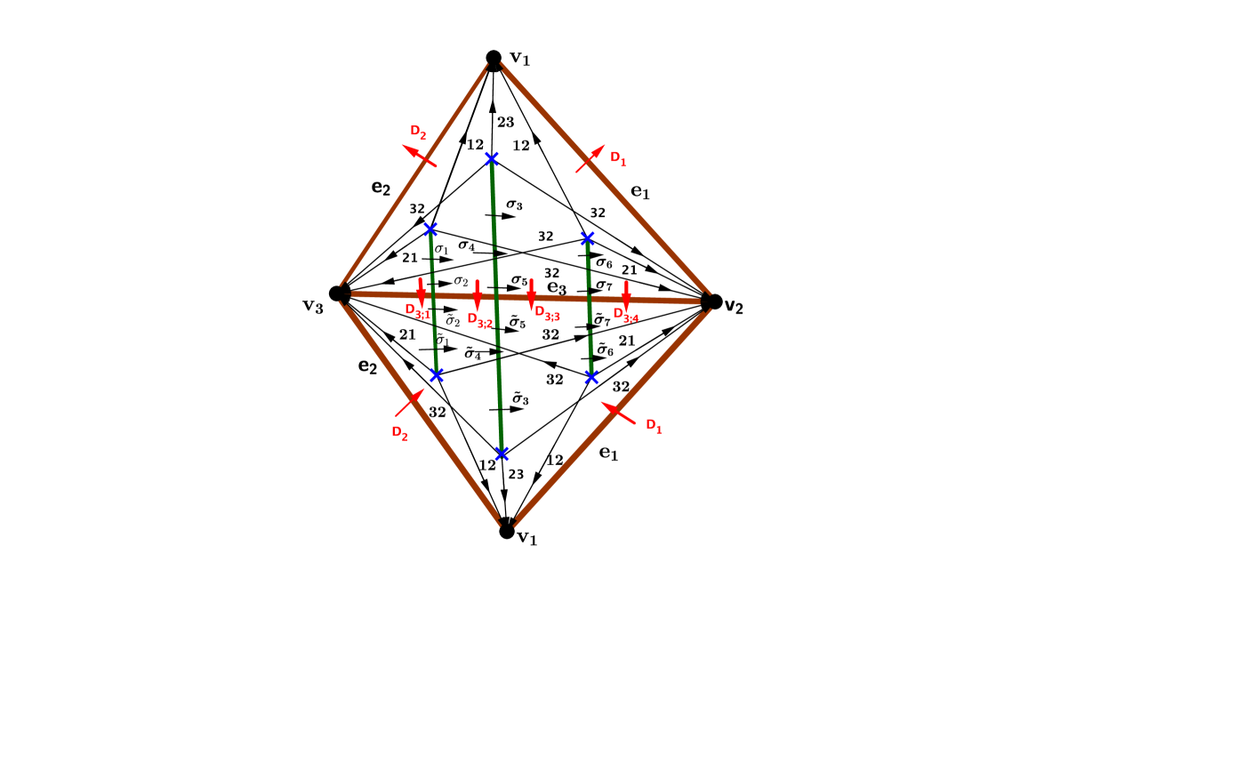
Figure 2: Traffic rule for $A_{2}$ theory on $\mathbb{P}^{1}/\{v_{1},v_{2},v_{3}\}$. The upper (lower) triangle is characterized by complex parameter $r_{2}$($r_{1}$).

In Figure 2 we give an example of the traffic rule for $A_{2}$ theory on $C=\mathbb{P}^{1}/\{v_{1},v_{2},v_{3}\}.$ To ensure the flatness of the connection, implying that monodromy is identity matrix around any contractible cycle on $\mathbb{P}^{1}/\{v_{1},v_{2},v_{3}\},$ we have to assign the following matrices to crossing various segments of the branch cuts

$$\sigma_{2}=S^{-1}_{12}S^{-1}_{21}(r_{2})S^{-1}_{32},\quad\tilde{\sigma}_{2}=S_{12}S_{21}(r_{1})S_{32}$$

$$\sigma_{5}=S^{-1}_{32}S^{-1}_{23}(r_{2})S^{-1}_{12}S^{-1}_{32}S_{12},\quad\tilde{\sigma}_{5}=S_{32}S_{23}(r_{1})S_{12}S_{32}S^{-1}_{12}$$ (1)

$$\sigma_{7}=S^{-1}_{32}S^{-1}_{21}(r_{2})S^{-1}_{12},\quad\tilde{\sigma}_{7}=S_{32}S_{21}(r_{1})S_{12}$$

For example, we compute

$$\sigma_{7}\sigma_{5}\sigma_{2}=M_{a}^{-1}(r_{2})M_{b}^{-1}(r_{2})S^{-1}_{32}S^{-1}_{21}(r_{2})S^{-1}_{32}=M_{a}^{-1}(r_{2})M_{b}^{-1}(r_{2})M_{a}^{-1}(r_{2}).$$

Here we used the matrices of crossing cables from [4]

$$M_{a}(r)=M_{c}(r)=S_{32}S_{21}(r)S_{32},\quad M_{b}(r)=S_{12}S_{23}(r)S_{12}.$$

The other crossing branch-cuts matrices are determined as follows:

$$\sigma_{1}=S^{-1}_{32}\sigma_{2}S_{32}\quad\sigma_{4}=S^{-1}_{32}\sigma_{5}S_{32}\quad\sigma_{3}=\sigma_{5}\quad\sigma_{6}=S_{32}\sigma_{7}S^{-1}_{32}$$ (2)

$$\tilde{\sigma}_{1}=S_{32}\tilde{\sigma}_{2}S^{-1}_{32}\quad\tilde{\sigma}_{4}=S_{32}\tilde{\sigma}_{5}S^{-1}_{32}\quad\tilde{\sigma}_{3}=\tilde{\sigma}_{5}\quad\tilde{\sigma}_{6}=S^{-1}_{32}\tilde{\sigma}_{7}S_{32}$$

We further introduce diagonal matrices $D_{(1)}$ and $D_{(2)}$ for crossing edges $e_{1}$ and $e_{2}$ which are not cut into segments by branch cuts. For the edge $e_{3},$ we introduce diagonal matrix $D_{(3;1)}$ for the crossing of the left-most segment of $e_{3}$ and compute from the requirement of flatness of the $GL(3,\mathbb{C})$ connection:

$$D_{(3;2)}=\tilde{\sigma}_{2}D_{(3;1)}\sigma_{2}^{-1},\quad D_{(3;3)}=\tilde{\sigma}_{5}D_{(3;2)}\sigma_{5}^{-1},\quad D_{(3;4)}=\tilde{\sigma}_{7}D_{(3;3)}\sigma_{7}^{-1}$$ (3)

Below we give explicit matrices used in crossing segment of branch cuts and edges:

$$\sigma_{1}=\begin{pmatrix}0&-1&0\cr 1&1&0\cr 1&1&r_{2}^{-1}\end{pmatrix},\quad\sigma_{2}=\begin{pmatrix}0&-1&0\cr 1&1&0\cr 0&r_{2}^{-1}&r_{2}^{-1}\end{pmatrix},\quad\sigma_{3}=\sigma_{5}=\begin{pmatrix}r_{2}^{-1}&0&0\cr 0&0&-1\cr 0&1&0\end{pmatrix}$$

$$\sigma_{4}=\begin{pmatrix}r_{2}^{-1}&0&0\cr 0&1&-1\cr 0&2&-1\end{pmatrix},\quad\sigma_{6}=\begin{pmatrix}1&-1&0\cr 1&0&0\cr 0&r_{2}^{-1}&r_{2}^{-1}\end{pmatrix},\quad\sigma_{7}=\begin{pmatrix}1&-1&0\cr 1&0&0\cr 1&0&r_{2}^{-1}\end{pmatrix}$$

$$\tilde{\sigma}_{1}=\begin{pmatrix}0&1&0\cr-1&1&0\cr 1&-1&r_{1}\end{pmatrix},\quad\tilde{\sigma}_{2}=\begin{pmatrix}0&1&0\cr-1&1&0\cr 0&-r_{1}&r_{1}\end{pmatrix},\quad\tilde{\sigma}_{3}=\tilde{\sigma}_{5}=\begin{pmatrix}r_{1}&0&0\cr 0&0&1\cr 0&-1&0\end{pmatrix}$$

$$\tilde{\sigma}_{4}=\begin{pmatrix}r_{1}&0&0\cr 0&1&1\cr 0&-2&-1\end{pmatrix},\quad\tilde{\sigma}_{6}=\begin{pmatrix}1&1&0\cr-1&0&0\cr 0&-r_{1}&r_{1}\end{pmatrix},\quad\tilde{\sigma}_{7}=\begin{pmatrix}1&1&0\cr-1&0&0\cr 1&0&r_{1}\end{pmatrix}$$

$$D_{(i)}=\begin{pmatrix}x_{i}&0&0\cr 0&y_{i}&0\cr 0&0&z_{i}\end{pmatrix},\quad i=1,2$$

$$D_{(3;1)}=\begin{pmatrix}x_{3}&0&0\cr 0&y_{3}&0\cr 0&0&z_{3}\end{pmatrix},\quad D_{(3;2)}=\begin{pmatrix}-y_{3}&0&0\cr-(x_{3}+y_{3})&-x_{3}&0\cr(y_{3}+z_{3})r_{1}&0&z_{3}r_{1}r_{2}\end{pmatrix}$$

$$D_{(3;3)}=\begin{pmatrix}-y_{3}r_{1}r_{2}&0&0\cr(y_{3}+z_{3})r_{1}r_{2}&-z_{3}r_{1}r_{2}&0\cr(x_{3}+y_{3})r_{2}&0&x_{3}\end{pmatrix},\quad D_{(3;4)}=r_{1}r_{2}\begin{pmatrix}z_{3}&0&0\cr 0&y_{3}&0\cr 0&0&x_{3}\end{pmatrix}$$

The traffic rule for $A_{2}$ theory on a more general $C$ is depicted on Figure 3, where we implicitly assume that matrices of crossing branch cuts depend on the parameter $r$ for the appropriate triangle. Figure 3 shows three rhombi, each built of a pair of triangles connected by three branch cuts. Finding traffic rule for a general $C,$ i.e. for any number of such rhombi, is very similar. This is the case due to our choice of branch cuts - three branch cuts are contained within each rhombus and no branch cuts go between different rhombi. So that one uses closed contours within each rhombus to determine matrices of crossing the branch cuts contained in the rhombus. Meanwhile, crossing the edges between different rhombi is described simply by diagonal matrices.

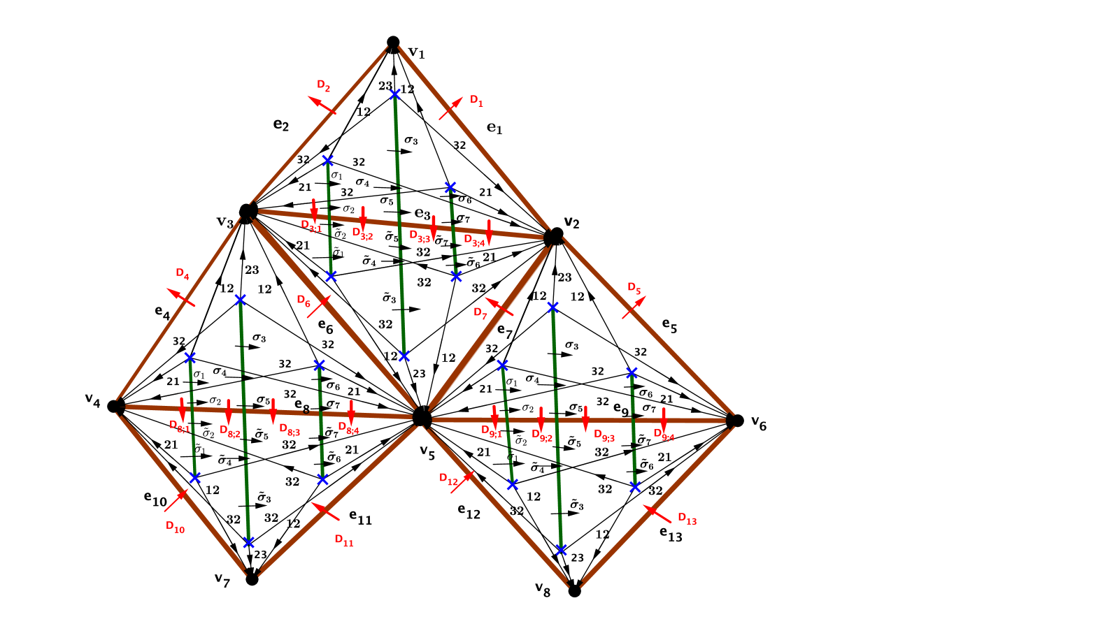
Figure 3: Traffic rule for minimal spectral network in general $A_{2}$ theory. It is implicitly assumed that matrices of crossing branch cuts depend on the parameter $r$ for the appropriate triangle.

We introduce diagonal matrices $D_{(1)},D_{(2)},D_{(4)},D_{(5)},D_{(6)},D_{(7)},D_{(10)},D_{(11)},D_{(12)},D_{(13)}$ for crossing the edges not split into segments by branch cuts as well as diagonal matrices $D_{(3;1)},D_{(8;1)},D_{(9;1)}$ for the left-most segments of the edges $e_{3},e_{8},e_{9}$ and compute similar to (3)

$$D_{(8;2)}=\tilde{\sigma}_{2}(r_{3})D_{(8;1)}\sigma_{2}(r_{4})^{-1},\quad D_{(8;3)}=\tilde{\sigma}_{5}(r_{3})D_{(8;2)}\sigma_{5}(r_{4})^{-1},\quad D_{(8;4)}=\tilde{\sigma}_{7}(r_{3})D_{(8;3)}\sigma_{7}(r_{4})^{-1}$$

$$D_{(9;2)}=\tilde{\sigma}_{2}(r_{5})D_{(9;1)}\sigma_{2}(r_{6})^{-1},\quad D_{(9;3)}=\tilde{\sigma}_{5}(r_{5})D_{(9;2)}\sigma_{5}(r_{6})^{-1},\quad D_{(9;4)}=\tilde{\sigma}_{7}(r_{5})D_{(9;3)}\sigma_{7}(r_{6})^{-1}$$

where we indicate the dependence on the appropriate $r_{i}$ parameters.

3.2 Monodromies around punctures

We are interested in flat $GL(3,\mathbb{C})$ connections with fixed conjugacy classes of the monodromies around the punctures. Let $P_{0}$ be a base point as shown in Figure 4. This choice will allow to introduce simplified network in Section 4. The closed paths, starting and ending at $P_{0},$ around $v_{1},v_{2},v_{3}$ are shown in Figure 4.

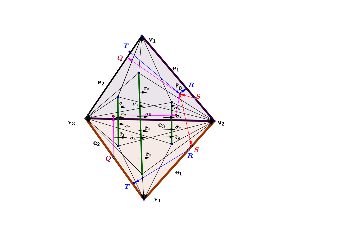
Figure 4: Monodromies around punctures with base point $P_{0}$

We use traffic rule formulated in the previous section to compute the corresponding monodromies

$$M_{P_{0}}(v_{1})=M^{-1}_{b}(r_{2})D^{-1}_{(2)}M^{-1}_{b}(r_{1})D_{(1)},\quad M_{P_{0}}(v_{2})=D^{-1}_{(1)}M^{-1}_{a}(r_{1})D_{(3;4)}M^{-1}_{a}(r_{2})$$ (4)

$$M_{P_{0}}(v_{3})=M_{a}(r_{2})W(r_{2})D^{-1}_{(3;1)}M^{-1}_{a}(r_{1})D_{(2)}M_{b}(r_{2})$$

where we denote $W(r_{2})=\sigma_{7}\sigma_{5}\sigma_{2}.$ These monodromies satisfy

$$M_{P_{0}}(v_{3})\,M_{P_{0}}(v_{1})\,M_{P_{0}}(v_{2})={\mathbb{I}}$$ (5)

Eigenvalues of these monodromies are

$$Eigen\Bigl{(}M_{P_{0}}(v_{1})\Bigr{)}=\Bigl{\{}{z_{1}\over z_{2}},{y_{1}\over y_{2}},{x_{1}\over x_{2}\,r_{1}\,r_{2}}\Bigr{\}}$$

$$Eigen\Bigl{(}M_{P_{0}}(v_{2})\Bigr{)}=\Bigl{\{}{x_{3}\over z_{1}},{r_{1}\,r_{2}\,y_{3}\over y_{1}},{r_{1}\,r_{2}\,z_{3}\over x_{1}}\Bigr{\}}$$

$$Eigen\Bigl{(}M_{P_{0}}(v_{3})\Bigr{)}=\Bigl{\{}{z_{2}\over z_{3}\,r_{1}\,r_{2}},{y_{2}\over y_{3}},{x_{2}\over x_{3}}\Bigr{\}}$$

Let us fix these eigenvalues in terms of masses $k_{j}\,j=1,\ldots,9$ such that $\prod_{j=1}^{9}k_{j}=1.$ Then, we find

$$r_{1}r_{2}=k_{2}k_{5}k_{8},\,z_{1}=k_{1}z_{2},\,z_{2}=x_{2}(k_{2}k_{3}k_{5}k_{6}k_{7}k_{8}),\,y_{1}=k_{2}y_{2},\,x_{1}=x_{2}(k_{2}k_{3}k_{5}k_{8})$$

$$x_{3}=k_{4}z_{1},\,y_{3}={y_{1}\over k_{2}k_{8}},\,z_{3}={x_{1}k_{6}\over k_{2}k_{5}k_{8}}$$

It follows that, for fixed masses $k_{j},$ monodromy around any closed path is a function of $r_{2}$ and $s={y_{2}\over x_{2}}.$

For example,

$$Tr\Bigl{(}M^{2}(v_{1})\,M(v_{2})\Bigr{)}=(k_{1}+k_{2}+k_{3})\left({1\over k_{7}}+{1\over k_{8}}+{1\over k_{9}}\right)+r_{2}\left(k_{1}k_{3}k_{4}+{k_{3}\over k_{8}}+{1\over k_{5}k_{8}k_{9}}\right)+$$

$${1\over r_{2}}\left(k_{1}k_{2}k_{5}+{k_{2}\over k_{7}}+{1\over k_{4}k_{7}k_{9}}\right)+s\left(k_{1}k_{2}k_{4}\left(1+{k_{9}\over k_{8}}\right)+{(k_{1}+k_{2})\over k_{8}}+{1\over k_{5}k_{7}k_{8}}+{1\over k_{6}k_{7}k_{8}}\right)+$$

$${1\over s}\left({k_{3}\over k_{9}}+{1\over k_{4}k_{7}k_{9}}\right)+{r_{2}\over s}\left({k_{3}\over k_{9}}\right)+{s\over r_{2}}\left(k_{1}k_{2}k_{5}+{k_{2}\over k_{3}k_{6}k_{7}k_{8}}+{k_{2}\over k_{7}}\right)+$$

$$r_{2}s\left({k_{1}k_{4}\over k_{5}k_{8}}+{1\over k_{5}k_{8}^{2}}+{k_{1}k_{3}k_{4}k_{9}\over k_{8}}\right)+{1\over r_{2}s}\left({1\over k_{4}k_{7}k_{9}}\right)+{s^{2}\over r_{2}}\left({k_{2}\over k_{3}k_{6}k_{7}k_{8}}\right)+s^{2}r_{2}\left({k_{1}k_{4}k_{9}\over k_{5}k_{8}^{2}}\right)+s^{2}\left({2k_{1}k_{2}k_{4}k_{9}\over k_{8}}\right)$$

Let us clarify the relation between coordinates $r_{2},s,k_{j}$ on $\mathcal{M}$ and Darboux coordinates reviewed in Section 2. The masses are identified with the center of the Poisson algebra:

$$X_{\gamma^{(1)}_{j}}=k_{j},\quad X_{\gamma^{(2)}_{j}}=k_{3+j},\quad X_{\gamma^{(3)}_{j}}=k_{6+j}\quad j=1,2,3.$$

It was shown in [4] that $X_{\beta}=r_{2}.$ Finally, $s={y_{2}\over x_{2}}$ is naturally identified with $X_{\alpha}$ since 1-cycle $\alpha$ intersects the edge $e_{2}$ once on sheet 1 and once on sheet 2 (with opposite orientation). This identification with Darboux coordinates implies

$$\{r_{2},s\}=r_{2}\,s.$$ (6)

So far we worked with local coordinates, but it turns out that $\mathcal{M}$ can be globally defined by 2 equations in 12 variables. Let us define

$$R_{1}=Tr\Bigl{(}M^{2}_{P_{0}}(v_{1})M_{P_{0}}(v_{2})\Bigr{)}-3,\quad R_{2}=Tr\Bigl{(}M^{2}_{P_{0}}(v_{2})M_{P_{0}}(v_{1})\Bigr{)}-3$$ (7)

$$L={1\over 3}Tr\Bigl{(}M^{2}_{P_{0}}(v_{2})M_{P_{0}}(v_{1})M^{-1}_{P_{0}}(v_{2})M^{-1}_{P_{0}}(v_{1})\Bigr{)}-{1\over 3}Tr\Bigl{(}M^{2}_{P_{0}}(v_{1})M_{P_{0}}(v_{2})M^{-1}_{P_{0}}(v_{1})M^{-1}_{P_{0}}(v_{2})\Bigr{)}$$ (8)

$$f_{a}^{j}=Tr\Bigl{(}M^{j}_{P_{0}}(v_{a})\Bigr{)}\quad a=1,2,3;\quad j=1,2,3.$$ (9)

The first of the two equations defining $\mathcal{M}$

$$\Bigl{(}\frac{1}{3}f_{1}^{3}+\frac{1}{6}(f_{1}^{1})^{3}-{\frac{1}{2}}f_{1}^{1}f_{1}^{2}\Bigr{)}\Bigl{(}\frac{1}{3}f_{2}^{3}+\frac{1}{6}(f_{2}^{1})^{3}-{\frac{1}{2}}f_{2}^{1}f_{2}^{2}\Bigr{)}\Bigl{(}\frac{1}{3}f_{3}^{3}+\frac{1}{6}(f_{3}^{1})^{3}-{\frac{1}{2}}f_{3}^{1}f_{3}^{2}\Bigr{)}=1$$ (10)

reflects the fact that $det\Bigl{(}M_{P_{0}}(v_{1})\Bigr{)}det\Bigl{(}M_{P_{0}}(v_{2})\Bigr{)}det\Bigl{(}M_{P_{0}}(v_{3})\Bigr{)}=1.$ The second equation states

$$L^{2}-u_{1}LR_{1}-u_{2}LR_{2}-u_{3}L-g_{1}R_{1}^{2}R_{2}^{2}-g_{2}R_{1}^{3}-g_{3}LR_{1}R_{2}-g_{4}R_{1}^{2}R_{2}-g_{5}R_{2}^{3}-g_{6}R_{2}^{2}R_{1}$$ (11)

$$-g_{7}R_{1}^{2}-g_{8}R_{2}^{2}-g_{9}R_{1}R_{2}-g_{10}R_{1}-g_{11}R_{2}-g_{12}=0$$

where $u_{1},\ldots,g_{12}$ are functions of $f_{a}^{j}.$ To get this equation we looked at the powers of $r_{2}$ and $s$ in each monomial $L^{n_{1}}R_{1}^{n_{2}}R_{2}^{n_{3}}$ with non-negative integers $n_{1},n_{2},n_{3}.$ Namely, we used that $L$ contains powers of $s$ not higher than $s^{3}$ and not lower than $s^{-3},$ and powers of $r_{2}$ not higher than $r_{2}^{2}$ and not lower than $r_{2}^{-2}.$ We further used that $R_{1}(R_{2})$ has powers of $s$ not higher than $s^{2}(s)$ and not lower than $s^{-1}(s^{-2}),$ and powers of $r_{2}$ not higher than $r_{2}$ and not lower than $r_{2}^{-1}.$So the procedure to get coefficients $g_{i}$ in (11) is to compute $L^{2}$ and first look at the monomial $s^{6}r_{2}^{4}.$ Besides $L^{2}$ only terms $g_{1}R_{1}^{2}R_{2}^{2}$ and $g_{3}LR_{1}R_{2}$ have such a monomial, so this gives equation for $g_{1},g_{3}.$ Then one looks at $s^{6}r_{2}^{3}$ etc. In Appendix we give coefficients $g_{i}$ for a simple case when all $f_{a}^{j}$ are parametrized by a single variable $n.$

From (10) and (11) we see that $\mathcal{M}$ has the structure of the fibration with the base defined by (10) and the fiber by (11). Note that the fiber is a non-compact complex surface in $\mathbb{C}^{3}.$ We discuss in details the special point in the base, the conformal point, in Section 5. At the conformal point the fiber is singular

$$L^{2}=R_{1}^{2}R_{2}^{2}-4(R_{1}+R_{2})^{3},$$

but away from this point the singularity is deformed, as we demonstrate in Appendix.

For the choice of the base point $P_{0}$ as in Figure 4, monodromies around punctures (4) can be expressed using simplified spectral network shown in Figure 5. Also, any closed curve with base point $P_{0}$ which can be drawn on Figure 4 is homotopic to a closed curve that can be drawn on a simplified Figure 5. We formulate the rules of the simplified network for general $C$ in Section 4.

4 Simplified spectral network for general $C$

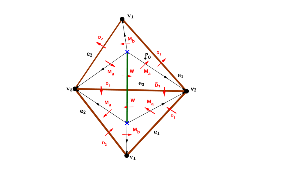
Figure 5: Simplified spectral network for $A_{2}$ theory on $\mathbb{P}^{1}/\{v_{1},v_{2},v_{3}\}$. $M_{a}(r),M_{b}(r)$ and $W(r)$ depend on the type of the spectral network -Yin or Yang- in a given triangle.

Any Riemann surface $C$ with punctures and without boundary can be triangulated by even number of triangles, and in each pair of triangles one can draw the simplified network shown in Figure 5. Moreover, in each triangle one may consider either Yin or Yang type of spectral network. In Section 3 we discussed in details Yin type networks but the story is similar for the Yang type. In a simplified network in Figure 5, the following matrices are used for Yin-type

$$M_{b}(r)=S_{12}\,S_{23}(r)\,S_{12}=\begin{pmatrix}r&1+r&1\cr 0&1&1\cr 0&0&1\end{pmatrix},\quad M_{a}(r)=S_{32}\,S_{21}(r)\,S_{32}=\begin{pmatrix}1&0&0\cr-1&1&0\cr 1&-(1+r)&r\end{pmatrix},$$

while for Yang-type

$$M_{b}(r)=S_{21}(r)\,S_{32}\,S_{21}(r)=\begin{pmatrix}1&0&0\cr-2&1&0\cr r&-r&r^{2}\end{pmatrix},\quad M_{a}(r)=S_{23}(r)\,S_{12}\,S_{23}(r)=\begin{pmatrix}r^{2}&r&r\cr 0&1&2\cr 0&0&1\end{pmatrix}.$$

In both types of triangles

$$W(r)=M_{a}^{-1}(r)M_{b}^{-1}(r)M_{a}^{-1}(r).$$ (12)

While in the Yin-type triangle this gives an off-diagonal matrix

$$W^{Yin}(r)={1\over r}\begin{pmatrix}0&0&1\cr 0&-1&0\cr 1&0&0\end{pmatrix},$$

this is not so in the Yang-type triangle

$$W^{Yang}(r)=\left(\begin{array}[]{ccc}\frac{2r^{2}-2r^{3}}{r^{6}}&\frac{-r^{5}+3r^{4}-2r^{3}}{r^{6}}&\frac{2r^{5}-4r^{4}+3r^{3}}{r^{6}}\\ \frac{2r^{4}-2r^{3}}{r^{6}}&\frac{r^{6}-4r^{5}+2r^{4}}{r^{6}}&\frac{-2r^{6}+6r^{5}-4r^{4}}{r^{6}}\\ \frac{1}{r^{3}}&\frac{r^{5}-r^{4}}{r^{6}}&\frac{2r^{4}-2r^{5}}{r^{6}}\\ \end{array}\right).$$

The simplified spectral network can be generalized for $A_{K}$ theory with $K>2$ by taking cable matrices $M_{a}(r),M_{b}(r),M_{c}(r)$ given in [4] and computing $W(r)$ from (12).

5 Space of line defects at the conformal point

Here we work at the conformal point in the base of $\mathcal{M}$ i.e. for $f_{a}^{j}=3$ for $a=1,2,3$ and $j=1,2,3.$ We investigate if the algebra of line defects in 4d theory is all of Functions on the fiber at the conformal point. For technical reasons, we do most of the computations in the Yin-Yin chart with coordinates $(r_{2},s)\in\mathbb{C}^{*}\times\mathbb{C}^{*}$ (see however expressions of the generators $R_{1},R_{2},L$ in the Yang-Yang chart at the end of this section). We conclude that traces of holonomies and webs together do not generate all of Functions of $(r_{2},s)\in\mathbb{C}^{*}\times\mathbb{C}^{*}.$ It is interesting that higher web-like structures, not previously discussed in the literature, correspond to line defects with vevs that are functionally independent of the vevs of defects arising from traces of holonomies.

Let us solve (5) as

$$M_{P_{0}}(v_{3})=M^{-1}_{P_{0}}(v_{2})M^{-1}_{P_{0}}(v_{1}),$$

simplify our notations $M_{j}=M_{P_{0}}(v_{j})$ and consider traces of words built from ‘letters’ $M_{1}^{\pm 1},M_{2}^{\pm 1}.$ We found that the space of these traces is generated by $R_{1},R_{2},L$ defined in (7-8). At the conformal point in the base they satisfy the relation

$$L^{2}=R_{1}^{2}R_{2}^{2}-4(R_{1}+R_{2})^{3}.$$ (13)

Let us denote line defects in 4d theory corresponding to certain linear combinations of traces of words as follows

$$\begin{array}[]{c|c}{\text{L}inear\,combination\,of\,words}&{\text{L}ine\,defect\,in\,4d}\cr 1&\hat{L}_{0}\cr Tr\Bigl{(}M_{1}^{2}M_{2}\Bigr{)}-3&\hat{L}_{1}\cr Tr\Bigl{(}M_{2}^{2}M_{1}\Bigr{)}-3&\hat{L}_{2}\cr\frac{1}{3}(I_{1}-I_{2})&\hat{L}_{3}\cr\frac{1}{3}(I_{1}+I_{2})&\hat{L}_{4}\cr\frac{1}{3}(J_{1}+J_{2})&\hat{L}_{5}\cr\frac{1}{3}(J_{1}-J_{2})&\hat{L}_{6}\cr\frac{1}{3}(\tilde{J}_{1}+\tilde{J}_{2})&\hat{L}_{9}\cr\frac{1}{3}(\tilde{J}_{1}-\tilde{J}_{2})&\hat{L}_{10}\cr Tr(M_{1}^{2}M_{2}M_{1}^{2}M_{2})&\hat{L}_{7}\cr Tr(M_{2}^{2}M_{1}M_{2}^{2}M_{1})&\hat{L}_{8}\cr\end{array}$$ (14)

where we denote

$$I_{1}=Tr\Bigl{(}M_{2}^{2}M_{1}M_{2}^{-1}M_{1}^{-1}\Bigr{)},\quad I_{2}=Tr\Bigl{(}M_{1}^{2}M_{2}M_{1}^{-1}M_{2}^{-1}\Bigr{)}$$

$$J_{1}:=Tr\Bigl{(}M_{2}M_{1}^{2}M_{2}^{2}M_{1}M_{2}^{-1}M_{1}^{-1}\Bigr{)},\quad J_{2}:=Tr\Bigl{(}M_{1}M_{2}^{2}M_{1}^{2}M_{2}M_{1}^{-1}M_{2}^{-1}\Bigr{)}$$

$$\tilde{J}_{1}:=Tr\Bigl{(}M_{1}^{2}M_{2}M_{1}^{2}M_{2}M_{1}^{-1}M_{2}^{-1}\Bigr{)},\quad\tilde{J}_{2}:=Tr\Bigl{(}M_{2}^{2}M_{1}M_{2}^{2}M_{1}M_{2}^{-1}M_{1}^{-1}\Bigr{)}$$

In terms of generators of traces:

$$Tr(M_{1}^{2}M_{2}M_{1}^{2}M_{2})=R_{1}^{2}+6R_{1}-2R_{2}+3,\quad Tr(M_{2}^{2}M_{1}M_{2}^{2}M_{1})=R_{2}^{2}+6R_{2}-2R_{1}+3$$

$$\frac{1}{3}(I_{1}+I_{2})=R_{1}R_{2}-4(R_{1}+R_{2})+2,\quad\frac{1}{3}(I_{1}-I_{2})=L$$

$$\frac{1}{3}(J_{1}+J_{2})=R_{1}R_{2}(R_{1}+R_{2})-6(R_{1}^{2}+R_{2}^{2})-10R_{1}R_{2}+2$$

$$\frac{1}{3}(J_{1}-J_{2})=(R_{1}+R_{2})L$$

$$\frac{1}{3}(\tilde{J}_{1}+\tilde{J}_{2})={\frac{1}{2}}R_{1}R_{2}(R_{1}+R_{2})+{\frac{1}{2}}(R_{2}-R_{1})L-2(R_{1}^{2}+R_{2}^{2})-R_{1}R_{2}-7(R_{1}+R_{2})+2$$

$$\frac{1}{3}(\tilde{J}_{1}-\tilde{J}_{2})=-{\frac{1}{2}}R_{1}R_{2}(R_{2}-R_{1})-{\frac{1}{2}}(R_{1}+R_{2})L+2(R_{2}^{2}-R_{1}^{2})-3L+(R_{1}-R_{2})$$

Let us define

$$\mathcal{L}_{0}=\hat{L}_{0},\quad\mathcal{L}_{1}=\hat{L}_{1}+\hat{L}_{2},\quad\mathcal{L}_{2}=\hat{L}_{2}-\hat{L}_{1},\quad\mathcal{L}_{3}=\hat{L}_{3}$$

We can build a nice basis of line defects $\mathcal{L}_{j}$ recursively by computing OPEs. For example:

$$\mathcal{L}_{1}\cdot\mathcal{L}_{1}=\mathcal{L}_{4},\quad\mathcal{L}_{2}\cdot\mathcal{L}_{2}=\mathcal{L}_{5},\quad\mathcal{L}_{1}\cdot\mathcal{L}_{2}=\mathcal{L}_{6}$$

$$\mathcal{L}_{2}\cdot\mathcal{L}_{3}=\mathcal{L}_{7},\quad\mathcal{L}_{1}\cdot\mathcal{L}_{3}=\mathcal{L}_{8}$$

where

$$\mathcal{L}_{4}=\hat{L}_{7}+\hat{L}_{8}+2\hat{L}_{4}+4(\hat{L}_{1}+\hat{L}_{2})-10\hat{L}_{0},\quad\mathcal{L}_{5}=\hat{L}_{7}+\hat{L}_{8}-2\hat{L}_{4}-4(\hat{L}_{1}+\hat{L}_{2})+10\hat{L}_{0}$$

$$\mathcal{L}_{6}=\hat{L}_{8}-\hat{L}_{7}-8(\hat{L}_{2}-\hat{L}_{1}),\quad\mathcal{L}_{7}=2\hat{L}_{9}-\hat{L}_{5}-2(\hat{L}_{7}+\hat{L}_{8})-8\hat{L}_{4}+4(\hat{L}_{1}+\hat{L}_{2})+10\hat{L}_{0},\quad\mathcal{L}_{8}=\hat{L}_{6}$$

In the Yin-Yin chart, i.e.when we choose the Yin-type spectral network in each of the two triangles, we find

$$R_{1}=\left(r_{2}+{1\over r_{2}}+2\right){(1+s)^{3}\over s},\,R_{2}=\left(r_{2}+{1\over r_{2}}+2\right){(1+s)^{3}\over s^{2}},\,L=\left({1\over r_{2}}-r_{2}\right)\left(r_{2}+{1\over r_{2}}+2\right){(1+s)^{6}\over s^{3}}$$ (15)

Note that there are two basic properties of the vevs of line defects corresponding to the traces. Substitution $M_{1}\leftrightarrow M_{2}$ in a word amounts to $r_{2}\leftrightarrow r_{2}^{-1}$ and $s\leftrightarrow s^{-1}$ in the vev. Substitution $M_{1}\leftrightarrow M_{1}^{-1},M_{2}\leftrightarrow M_{2}^{-1}$ in a word has similar effect on the vev.

The generators transform as

$$R_{1}\leftrightarrow R_{2},\quad L\mapsto-L\quad\text{under}\quad r_{2}\leftrightarrow r_{2}^{-1},\,s\leftrightarrow s^{-1}.$$

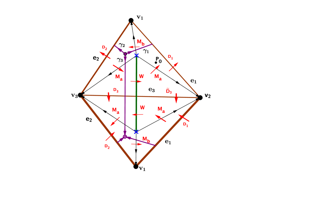
Figure 6: Web $W_{1}$

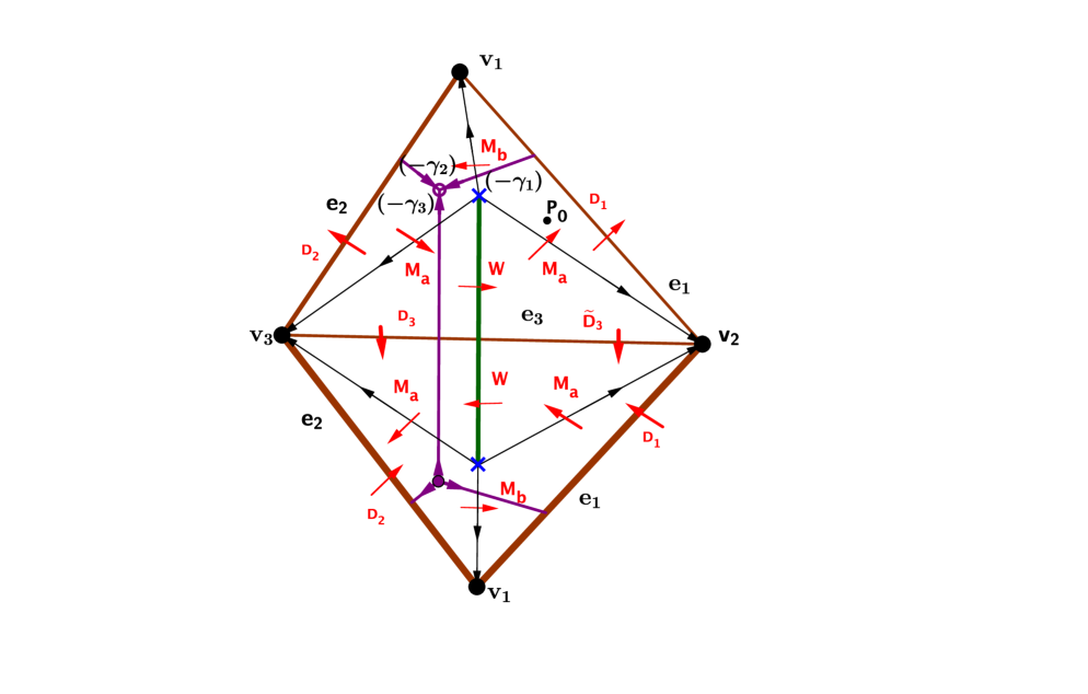
Figure 7: Web $W_{2}$

As argued in [9, 10], the space of line defects in 4d theory also includes defects corresponding to webs. The two examples of webs are shown in Figure 6 and Figure 7. They give line defects with the following vevs:

$$W_{1}=6-R_{1},\quad W_{2}=6-R_{2}.$$ (16)

We computed these from the following gauge-invariant expressions:

$$W_{1}={web_{1}\over detM_{\gamma_{1}}}\quad web_{1}=\epsilon_{i_{1}j_{1}k_{1}}\epsilon^{i_{2}j_{2}k_{2}}\left(M_{\gamma_{1}}\right)^{i_{1}}_{i_{2}}\,\left(M_{\gamma_{2}}\right)^{j_{1}}_{j_{2}}\,\left(M_{\gamma_{3}}\right)^{k_{1}}_{k_{2}}$$

$$W_{2}=web_{2}\,detM_{\gamma_{1}}\quad web_{2}=\epsilon_{i_{1}j_{1}k_{1}}\epsilon^{i_{2}j_{2}k_{2}}\left(M^{-1}_{\gamma_{1}}\right)^{i_{1}}_{i_{2}}\,\left(M^{-1}_{\gamma_{2}}\right)^{j_{1}}_{j_{2}}\,\left(M^{-1}_{\gamma_{3}}\right)^{k_{1}}_{k_{2}}$$

where

$$M_{\gamma_{1}}=M_{b}(r_{1})^{-1}\,D_{(1)}\,M_{b}(r_{2})^{-1},\quad M_{\gamma_{2}}=D_{(2)},\quad M_{\gamma_{3}}=M_{a}(r_{1})\,D_{(3)}\,M_{a}(r_{2}).$$

Note that $W_{1}$ and $W_{2}$ are linear combination of traces of holonomies. It is also interesting that another web $W_{3}$ (see Figure 8) gives the same vev as $W_{1}$ only at the conformal point. Away from the conformal point the vev of $W_{3}$ differs as function of masses from the vev of $W_{1}.$

Two more examples of basic webs are $W_{4}$ (see Figure 9) and $W_{5}$ obtained from $W_{4}$ by reversing the arrows. They give vevs that are again linear combinations of traces of holonomies;

$$W_{4}=6-R_{2},\quad W_{5}=6-R_{1}.$$

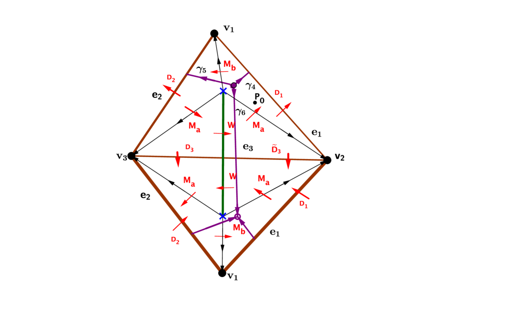
Figure 8: Web $W_{3}$

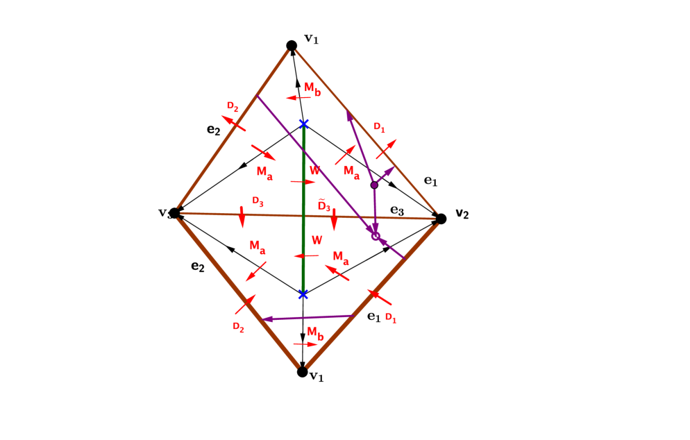
Figure 9: Web $W_{4}$

There are line defects arising from more complicated web-like structures. For example, the structure depicted in Figure 10 gives the vev

$$\mathbf{W}={{\epsilon}^{i_{1}j_{1}n}\,{\epsilon}_{i_{2}j_{2}t}\,{\epsilon}^{p_{1}p_{2}m}\,{\epsilon}_{q_{1}q_{2}s}\,\left(U^{(\gamma_{1})}\right)_{i_{1}}^{i_{2}}\,\left(U^{(\gamma_{2})}\right)_{j_{1}}^{j_{2}}\,\left(U^{(\gamma_{6})}\right)_{p_{1}}^{q_{1}}\,\left(U^{(\gamma_{3})}\right)_{p_{2}}^{q_{2}}\,\left(U^{(\gamma_{5})}\right)_{n}^{s}\,\left(U^{(\gamma_{4})}\right)_{m}^{t}\over det\,U^{(\gamma_{4})}\,det\,U^{(\gamma_{5})}}$$

where using traffic rule we computed

$$U^{(\gamma_{1})}=D_{(2)}^{-1}M^{-1}_{b}(r_{1})D_{(1)},\quad U^{(\gamma_{2})}=M^{-1}_{a}(r_{2})W^{-1}(r_{2})M^{-1}_{a}(r_{2}),\quad U^{(\gamma_{3})}=M^{-1}_{a}(r_{1})W^{-1}(r_{1})M^{-1}_{a}(r_{1}),$$

$$U^{(\gamma_{4})}=D_{(2)}^{-1},\quad U^{(\gamma_{5})}=D_{(1)},\quad U^{(\gamma_{6})}=M_{b}(r_{1})$$

So that at the conformal point the vev is

$$\mathbf{W}=10-{8\over r_{2}}.$$

Reversing all the arrows gives another web, shown in Figure 11, which gives the vev

$$\overline{\mathbf{W}}=10-8r_{2}.$$

We see that $\mathbf{W}$ and $\overline{\mathbf{W}}$ are independent as functions of $(r_{2},s)$ from the traces of holonomies. Let us give another example of more complicated web-like structure (see Figure 12)

$$\widehat{\mathbf{W}}=-21-\frac{3}{r_{2}}-r_{2}+5r_{2}^{2}-\frac{5}{s}-\frac{1}{r_{2}s}-\frac{3r_{2}}{s}+\frac{r_{2}^{2}}{s}-3s-\frac{3s}{r_{2}}+7r_{2}s+7r_{2}^{2}s+s^{2}-\frac{s^{2}}{r_{2}}+5r_{2}s^{2}+3r_{2}^{2}s^{2}$$

that is also independent of the traces of holonomies.

Figure 10: More complicated web-like structure $\mathbf{W}$

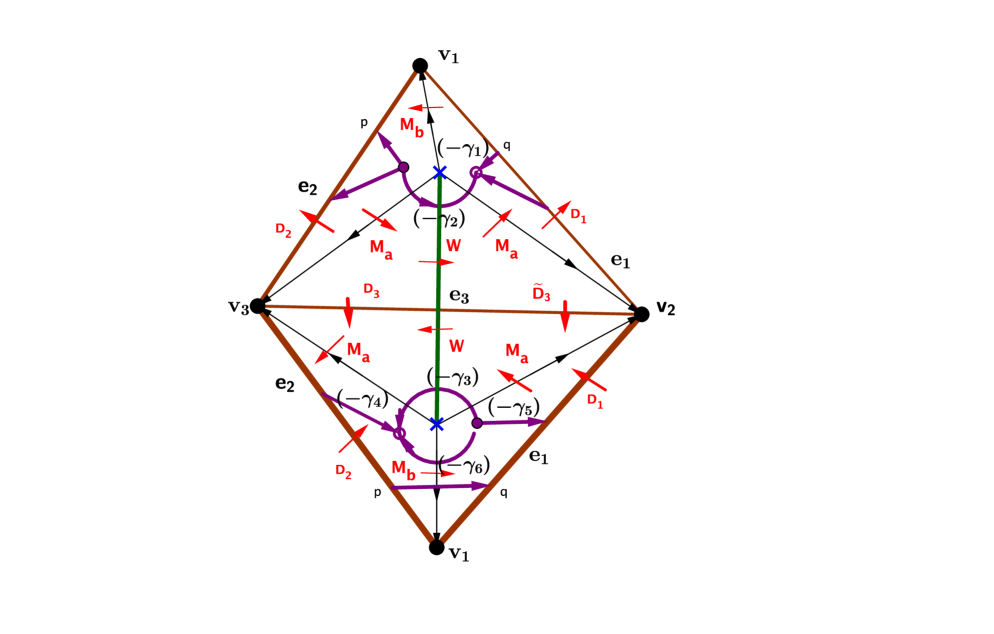
Figure 11: More complicated web-like structure with $\overline{\mathbf{W}}$

Figure 12: More complicated web-like structure $\widehat{\mathbf{W}}$

Note that we could not find a web-like structure, nor basic neither more complicated, which gives just linear dependence in $s$ without any dependence on $r_{2}$. Hence we conclude that we do not get all Functions of $(r_{2},s)$ from traces of holonomies and web-like structures.

We finish this section with a comment about the Yang-Yang chart. Requiring that all eigenvalues of monodromies around punctures are 1, gives

$$x_{1}=x_{2}=x_{3},\quad y_{1}=y_{2}=y_{3},\quad z_{1}=z_{2}=z_{3},\quad r_{1}r_{2}=1$$

and relation

$$6-{4\over r_{2}}-4r_{2}+{2\over s}-{2\over r_{2}s}+2s-{2s\over r_{2}}+{1\over s_{2}}+{2s\over s_{2}}-{2r_{2}s\over s_{2}}+s_{2}+{2s_{2}\over s}-{2r_{2}s_{2}\over s}=0$$ (17)

where

$$s_{2}={z_{2}\over x_{2}},\quad s_{1}={y_{2}\over x_{2}}.$$

So that in the Yang-Yang chart all traces (at the conformal point) are functions of $s_{1},s_{2}$ with $r_{2}$ determined from the relation (17).

For example, the generators of the traces are expressed in this chart as

$$R_{1}=\frac{2(s_{1}+1)(s_{1}+s_{2})(s_{2}+1+2s_{1})}{s_{1}s_{2}}$$ (18)

$$R_{2}=\frac{2(s_{1}+1)(s_{1}+s_{2})(s_{1}s_{2}+2s_{2}+s_{1})}{s_{1}^{2}s_{2}}$$ (19)

$$L=\frac{4(s_{1}+1)^{2}(s_{1}+s_{2})^{2}\left(s_{1}^{2}(-4r_{2}+2s_{2}+2)+s_{1}\left((6-8r_{2})s_{2}+s_{2}^{2}+1\right)+2s_{2}(-2r_{2}s_{2}+s_{2}+1)\right)}{s_{1}^{3}s_{2}^{2}}$$

6 Relation with Fock-Goncharov variables

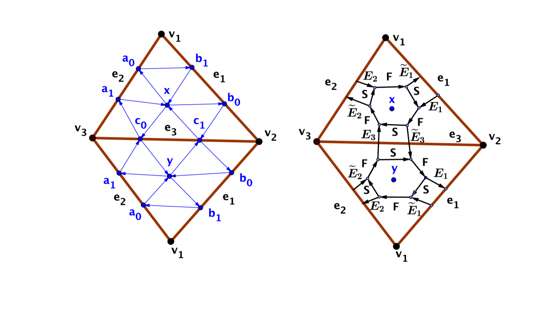
Figure 13: Fock-Goncharov variables and monodromy graph for $A_{2}$ theory on $\mathbb{P}^{1}/\{v_{1},v_{2},v_{3}\}$

The Fock-Goncharov variables and monodromy graph [8] for moduli space of $PGL(3,\mathbb{C})$ connections on $\mathbb{P}^{1}/\{v_{1},v_{2},v_{3}\}$ are depicted in Figure 4. The non-zero Poisson brackets are

$$\{x,a_{0}\}=xa_{0},\quad\{x,a_{1}\}=-xa_{1},\quad\{x,b_{0}\}=xb_{0},\quad\{x,b_{1}\}=-xb_{1},\quad\{x,c_{0}\}=xc_{0},\quad\{x,c_{1}\}=-xc_{1}$$ (20)

$$\{y,a_{0}\}=-ya_{0},\quad\{y,a_{1}\}=ya_{1},\quad\{y,b_{0}\}=-yb_{0},\quad\{y,b_{1}\}=yb_{1},\quad\{y,c_{0}\}=-yc_{0},\quad\{y,c_{1}\}=yc_{1}$$

Let us write monodromies around punctures (see Figure 14) with the same base point $P_{0}$ that we used in computing the corresponding monodromies in spectral network set up.

$$M^{FG}_{P_{0}}(v_{1})=S\,F(x)\,E_{2}\,F(y)\,S\,E_{1}^{-1}$$

$$M^{FG}_{P_{0}}(v_{2})=E_{1}\,F(y)\,\tilde{E}_{3}\,F(x)$$

$$M^{FG}_{P_{0}}(v_{3})=F^{-1}(x)\,S\,E_{3}\,F(y)\,\tilde{E}_{2}\,S\,F^{-1}(x)\,S$$

where

$$S=\begin{pmatrix}0&0&-1\cr 0&1&0\cr-1&0&0\cr\end{pmatrix},\quad F(x)=\begin{pmatrix}x&0&0\cr x&x&0\cr x&x+1&1\end{pmatrix},\quad E_{1}=\begin{pmatrix}b_{0}b_{1}&0&0\cr 0&b_{1}&0\cr 0&0&1\end{pmatrix},\quad\tilde{E}_{1}=\begin{pmatrix}b_{0}b_{1}&0&0\cr 0&b_{0}&0\cr 0&0&1\end{pmatrix},\quad$$

$$E_{2}=\begin{pmatrix}a_{0}a_{1}&0&0\cr 0&a_{1}&0\cr 0&0&1\end{pmatrix},\quad\tilde{E}_{2}=\begin{pmatrix}a_{0}a_{1}&0&0\cr 0&a_{0}&0\cr 0&0&1\end{pmatrix},\quad E_{3}=\begin{pmatrix}c_{0}c_{1}&0&0\cr 0&c_{1}&0\cr 0&0&1\end{pmatrix},\quad\tilde{E}_{3}=\begin{pmatrix}c_{0}c_{1}&0&0\cr 0&c_{0}&0\cr 0&0&1\end{pmatrix},\quad$$

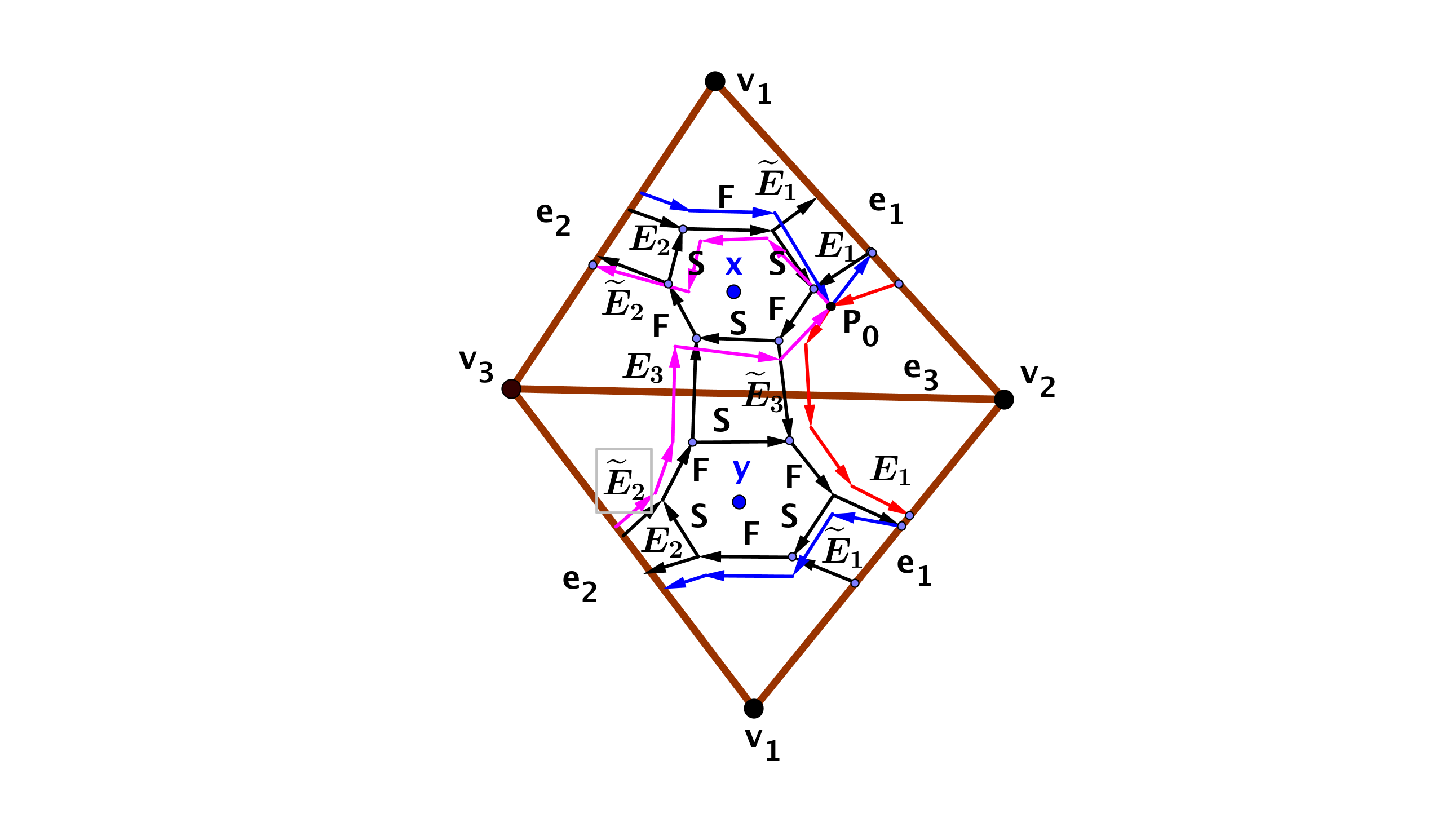
Figure 14: Monodromies around punctures in Fock-Goncharov variables for $A_{2}$ theory on $\mathbb{P}^{1}/\{v_{1},v_{2},v_{3}\}$

To write down eigenvalues (defined up to a scale) of these monodromy matrices, it is convenient to introduce the following combinations of FG variables

$$\Upsilon^{(1)}_{1}=a_{0}b_{1},\,\Upsilon^{(1)}_{2}=a_{1}b_{0},\,\Upsilon^{(2)}_{1}=b_{0}c_{1},\,\Upsilon^{(2)}_{2}=b_{1}c_{0},\,\Upsilon^{(3)}_{1}=a_{1}c_{0},\,\Upsilon^{(3)}_{2}=a_{0}c_{1},\,f=xy.$$

Note the relation:

$$\Upsilon_{1}^{(1)}\,\Upsilon_{1}^{(2)}\,\Upsilon_{1}^{(3)}\,=\,\Upsilon_{2}^{(1)}\,\Upsilon_{2}^{(2)}\,\Upsilon_{2}^{(3)}$$ (21)

We find the eigenvalues

$$\bigl{(}n^{(a)}_{1},n^{(a)}_{2},n^{(a)}_{3}\bigr{)}:=Eigen\Bigl{(}M^{FG}_{P_{0}}(v_{a})\Bigr{)}=\Lambda^{(a)}\bigl{(}1,\xi^{(a)}_{1},\xi^{(a)}_{2}\bigr{)}\quad a=1,2,3.$$

where $\Lambda^{(a)}$ are arbitrary scale factors and

$$\xi^{(a)}_{1}=f\Upsilon^{(a)}_{1},\quad\xi^{(a)}_{2}=f\Upsilon^{(a)}_{1}\Upsilon^{(a)}_{2}.$$ (22)

As a consequence of (21):

$$f^{3}={\left(\xi^{(1)}_{2}\,\xi^{(2)}_{2}\,\xi^{(3)}_{2}\right)^{2}\over\xi^{(1)}_{1}\,\xi^{(2)}_{1}\,\xi^{(3)}_{1}}.$$ (23)

For each puncture let us compute the two invariant (under rescaling and Weyl group action) combinations

$$\rho^{(a)}_{1}={\Bigl{(}n^{(a)}_{1}+n^{(a)}_{2}+n^{(a)}_{3}\Bigr{)}^{3}\over n^{(a)}_{1}\,n^{(a)}_{2}\,n^{(a)}_{3}}={\Bigl{(}1+\xi^{(a)}_{1}+\xi^{(a)}_{2}\Bigr{)}^{3}\over\xi^{(a)}_{1}\,\xi^{(a)}_{2}}$$ (24)

$$\rho^{(a)}_{2}={\Bigl{(}n^{(a)}_{1}+n^{(a)}_{2}+n^{(a)}_{3}\Bigr{)}\Bigl{(}n^{(a)}_{1}n^{(a)}_{2}+n^{(a)}_{2}n^{(a)}_{3}+n^{(a)}_{1}n^{(a)}_{3}\Bigr{)}\over n^{(a)}_{1}\,n^{(a)}_{2}\,n^{(a)}_{3}}={\Bigl{(}1+\xi^{(a)}_{1}+\xi^{(a)}_{2}\Bigr{)}\Bigl{(}\xi^{(a)}_{1}+\xi^{(a)}_{2}+\xi^{(a)}_{1}\xi^{(a)}_{2}\Bigr{)}\over\xi^{(a)}_{1}\,\xi^{(a)}_{2}}$$

Now it is clear how to explicutly relate Fock-Goncharov and spectral network variables. We first compute $\rho^{(a)}_{1},\rho^{(a)}_{2}$ from spectral network, i.e. as functions of masses $k_{i}.$ Then we find $\xi^{(a)}_{1},\xi^{(a)}_{2}$ from $\rho^{(a)}_{1},\rho^{(a)}_{2},$ compute $f$ from (23) and determine $\Upsilon^{(a)}_{1},\Upsilon^{(a)}_{2}$ from (22). Finally, let us recall the relation between FG variables and $f,\Upsilon^{(a)}_{1},\Upsilon^{(a)}_{2}$ (21) and Poisson brackets (20). This allows to write an explicit map

$$a_{0}=s,\,x=r_{2},\,y={f\over r_{2}},\,b_{1}={\Upsilon_{1}^{(1)}\over s},\,c_{1}={\Upsilon_{2}^{(3)}\over s},\,c_{0}={s\,\Upsilon_{2}^{(2)}\over\Upsilon_{1}^{(1)}},\,a_{1}={\Upsilon_{1}^{(3)}\Upsilon_{1}^{(1)}\over s\Upsilon_{2}^{(2)}},\,b_{0}={s\,\Upsilon_{1}^{(2)}\over\Upsilon_{2}^{(3)}}$$ (25)

The only technical difficulty arises in solving for $\xi^{(a)}_{1},\xi^{(a)}_{2}$ from $\rho^{(a)}_{1},\rho^{(a)}_{2}.$ One may first determine $\mu^{(a)}=\xi^{(a)}_{1}\xi^{(a)}_{2}$ and $\nu^{(a)}=\xi^{(a)}_{1}+\xi^{(a)}_{2}+1$ and then solve quadratic equation to find $\xi$’s from $\mu$ and $\nu.$ Note that from (24)

$$\mu^{(a)}={\left(\nu^{(a)}\right)^{3}\over\rho_{1}^{(a)}}$$

and $\nu^{(a)}$ is a solution of a cubic equation for each puncture $a=1,2,3$

$$\left(\nu^{(a)}\right)^{3}-\rho_{2}^{(a)}\left(\nu^{(a)}\right)^{2}+\rho_{1}^{(a)}\nu^{(a)}-\rho_{1}^{(a)}=0.$$

7 Acknowledgments

I am very grateful to Greg Moore for many valuable advices without which this work would not be possible. I would like to express my thanks to the Aspen Center for Physics for hospitality during July 2013.

8 Appendix

Let us consider a deviation from the conformal point in the base of $\mathcal{M}$ parametrized as

$$f_{1}^{1}=n+2;\quad f_{1}^{2}=n^{2}+2;\quad f_{1}^{3}=n^{3}+2;\quad f_{2}^{j}=3;\quad f_{3}^{1}=n^{-1}+2;\quad f_{3}^{2}=n^{-2}+2;\quad f_{3}^{3}=n^{-3}+2.$$

Below we provide coefficients of the equation (11) for this simple deviation.

$$g_{1}=\frac{n+2}{3n^{2}};\quad g_{3}=\frac{-n^{2}-4n+5}{3n^{2}+15n};\quad u_{1}=\frac{3n^{3}+13n^{2}-11n-5}{3n^{2}+15n};$$

$$g_{2}=\frac{-n^{2}-10n-25}{9n^{2}};\quad g_{4}=\frac{-3n^{3}+3n^{2}u_{1}-23n^{2}+6nu_{1}-47n-35}{9n^{2}};$$

$$g_{6}=\frac{-n^{5}-11n^{4}+3n^{3}u_{2}-38n^{3}+6n^{2}u_{2}-43n^{2}-15n}{9n^{3}};\quad u_{2}=\frac{n^{5}+8n^{4}+10n^{3}-24n^{2}+5n}{3n^{3}+15n^{2}};$$

$$g_{5}=\frac{-n^{4}-10n^{3}-25n^{2}}{9n^{3}};\quad g_{7}=\frac{2n^{2}}{9}-\frac{119}{9n^{2}}+\frac{46n}{9}-\frac{4}{n}+\frac{107}{9};$$

$$g_{9}=\frac{34n^{4}+157n^{3}+108n^{2}-175n-124}{9n^{2}};$$

$$g_{10}=\frac{-n^{6}-58n^{5}-171n^{4}+91n^{3}+380n^{2}-53n-188}{9n^{2}};$$

$$g_{11}=\frac{-15n^{6}-100n^{5}-119n^{4}+226n^{3}+293n^{2}-198n-87}{9n^{2}};$$

$$g_{8}=\frac{3n^{5}+30n^{4}+87n^{3}+29n^{2}-130n-19}{9n^{2}};u_{3}=\frac{-3n^{5}-17n^{4}+46n^{2}-21n-5}{3n^{2}+15n};$$

$$g_{12}=\frac{(n-1)^{2}\left(22n^{5}+130n^{4}+206n^{3}-25n^{2}-240n-94\right)}{9n^{2}}$$

We find that for generic $n$ the fiber of $\mathcal{M}$ is a non-singular complex surface in $\mathbb{C}^{3}.$

References

• [1] D.Β Gaiotto, G.Β Moore, A.Β Neitzke, β€œWall-crossing, Hitchin Systems, and the WKB Approximation”, [arXiv:0907.3987]
• [2] N. Β Nekrasov, A. Β Rosly, S.Β Shatashvili, β€œDarboux coordinates, Yang-Yang functional, and gauge theory”, Nucl.Phys.Proc.Suppl.Β 216, p. 69,Β  [arXiv:1103.3919].
• [3] D.Β Gaiotto, G.Β Moore, A.Β Neitzke, β€œSpectral networks”, [arXiv:1204.4824]
• [4] D.Β Gaiotto, G.Β Moore, A.Β Neitzke, β€œSpectral networks and snakes”, [arXiv:1209.0866]
• [5] D. P. Thurston, unpublished.
• [6] R. C. Penner ,β€œThe decorated Teichmuller space of Riemann surfaces ”, Comm.Math.Phys., 113(1988), 299 339.
• [7] V. Fock, A. Goncharov, β€œDual Teichmuller and lamination spaces”, [arXiv:math/0510312].
• [8] V. Fock, A. Goncharov, β€œModuli spaces of local systems and higher Teichmuller theory”, [arXiv:math/0311149].
• [9] D. Xie, β€œHigher laminations, webs and N=2 line operators”, [arXiv:1304:2390].
• [10] D. Xie, β€œAspects of line operators of class S theories”, [arXiv:1312:3371].