Root Finding by High Order Iterative Methods Based on Quadratures

Abstract

We discuss a recursive family of iterative methods for the numerical approximation of roots of nonlinear functions in one variable. These methods are based on Newton-Cotes closed quadrature rules. We prove that when a quadrature rule with $n+1$ nodes is used the resulting iterative method has convergence order at least $n+2$, starting with the case $n=0$ (which corresponds to the Newton’s method).

1 Introduction

The use of quadrature rules for the construction of iterative methods, applied to the solution of nonlinear equations or systems, has been considered by many authors (see, for example, [22], [6], [11], [16]). However, so far these methods have in general been treated separately or dealing with a specific quadrature rule or a small set of them. In this work we shall treat this matter in a systematic and unifying way.

Our main purpose is to obtain a family of recursive iterative methods based on quadratures, with higher convergence order than the Newton’s method. This one is universally considered the method of choice for approximating a root $z\in\mathbb{R}^{d}$ for a given equation $f(x)=0$, where $f:D\subset\mathbb{R}^{d}\mapsto\mathbb{R}^{d}$. However, its limitations are also known. In many cases of practical interest, the Newton’s method fails to converge unless the initial approximation lies in a small neighborhood of the root we want to approximate. It’s mainly in such cases that higher order iterative methods can be useful, such as those described in the present paper.

For a fixed positive integer $n$, we define recursively a certain function $t_{n}:\mathbb{R}\mapsto\mathbb{R}$, based on a Newton-Cotes closed quadrature rule, with $n+1$ nodes (see Definition 2.1). Numerical integration is discussed, for example, in [14] Ch. 6, [2] Ch. 5, and for Newton-Cotes quadrature rules, see for instance [7], Ch. 3, and [10].

In the present work, we take as the basic iteration function $t_{0}$ the Newton’s iterative process. Assuming that the Newton’s method has convergence order $p\geq 2$, we prove in Theorem 3.1 that the convergence order of our iterative function $t_{n}$ is not less than $2+n$. This enables us to construct iterative methods of arbitrary convergence order for the numerical solution of nonlinear equations.

In Sec. 2 we establish a relation between the approximation of a real root $z$ of an equation $f(x)=0$ and a quadrature rule, using the main theorem of integral calculus. Though we restrict ourselves to closed Newton-Cotes rules, quadratures of different types can be also used.

The iterative methods described here can be easily extended to the case of multivariate functions. However, the analysis of convergence in this case is out of the scope of the present paper.

In Sec. 3 we begin by showing that the iterative function $t_{0}$ coincides with the classical Newton’s iterative function. As known, if $z$ is a simple root, this process has at least second order convergence, provided that the initial approximation is sufficiently close to a simple root $z$. For a given integer $n\geq 1$, we show how to apply a certain closed Newton-Cotes quadrature rule (with $n+1$ nodes), in order that the corresponding recursive iterative method, $t_{n}$, possesses in general a higher convergence order than the previous iterative mapping $t_{n-1}$. Namely, we prove that each iterative mapping $t_{n}$ has convergence order not less than $n+2$, which is the main result of this work.

In Sec. 4 we present some numerical examples illustrating the application of the described methods. We compare their accuracy and verify experimentally their convergence order. Special attention is paid to the cases where the classical Newton’s method fails.

Finally, in Sec. 5, we present the main conclusions and discuss perspectives for a future work.

2 Iterative Methods for Root Finding and Quadrature Rules

Given a function $f$ in one real variable, let $z$ be a simple root of $f$ (that is $f^{\prime}(z)\neq 0$). Suppose that $f$ is sufficiently regular in a certain neighborhood of $z$. By the fundamental theorem of integral calculus we know that

$$\int_{x}^{z}f^{(1)}(t)\,dt=f(z)-f(x)=-f(x).$$ (1)

Choosing a non-negative integer $n$, we approximate the integral on the left-hand side of (1) by a certain interpolatory quadrature rule with $n+1$ nodes, which we denote by $Q_{n}\left(f^{(1)}\right)$. We can write the rule as

$$Q_{n}\left(f^{(1)}\right)=\displaystyle{\frac{z-x}{c_{n}}}\,B_{n}(x).$$ (2)

The function $B_{n}(x)$ in (2) is defined by the weights $A_{i}$ and by the “nodes”$\,\xi_{i}(x)\in[x,z]$, such that

$$B_{n}(x)=A_{0}\,f^{(1)}(\xi_{0}(x))+A_{1}\,f^{(1)}(\xi_{1}(x))+\cdots+A_{n}\,f^{(1)}(\xi_{n}(x)).$$ (3)

In an interpolatory quadrature rule, the constant $c_{n}$ in (2) satisfies the equality

$$c_{n}=\sum_{i=0}^{n}A_{i},$$ (4)

since, by construction, the rule is exact when applied to $f(x)\equiv 1$.

We also assume that for $t\in[x,z]$, the function $B_{n}(t)$ is finite and has a finite inverse, that is,

$$B_{n}(t)\neq 0\quad\forall t\in[x,z].$$ (5)

Finally, the quadrature nodes $\xi_{i}(x)$ satisfy

$$\xi_{i}(z)=z,\quad\mbox{para}\quad i=0,1,\ldots,n.$$ (6)

In Sec. 3 we will define the functions $\xi_{i}(x)$, which are the quadrature nodes in (3), using the closed Newton-Cotes quadrature rules ([7], Ch. 3).

The iterative processes to be constructed will possess some of the properties of the adopted quadrature rules, and this will be reflected in the following proofs. In a future work we intend to use open quadrature rules with the same purpose.

Substituting (2) into (1), we obtain

$$z-x\simeq-c_{n}\,B_{n}^{-1}(x)\,f(x).$$ (7)

The approximate equality (7) leads us to the following definition of the mapping $t_{n}$.

Definition 2.1

(Iterative mapping based on a quadrature rule)

For a given integer $n\geq 0$ and a certain function $B_{n}(x)$, associated to the quadrature rule (2), satisfying the conditions (3)-(6), the iterative mapping $t_{n}$ is defined by

$$t_{n}(x)=x-c_{n}\,B_{n}^{-1}(x)f(x).$$ (8)

Defining the auxiliary function

$$H_{n}(x)=t_{n}(x)-x,$$ (9)

we remark that $H_{n}$ satisfies

$$B_{n}(x)\,H_{n}(x)=-c_{n}\,f(x)\Longleftrightarrow H_{n}(x)=-c_{n}\,B_{n}^{-1}(x)\,f(x).$$ (10)

Since, for $n\geq 1$, we will use only closed Newton-Cotes quadrature rules, the function $t_{n}$ in (8) will be called the Newton-Cotes closed iterative mapping with $n+1$ nodes.

We begin by proving the superlinear convergence of the mapping defined by (8), in the case $f$ is a one-variable function, sufficiently regular in the neighborhood of a simple root $z$.

Proposition 2.1

(Superlinear convergence of iterating mappings)

A simple root of the equation $f(x)=0$ is a fixed point of the iterative mapping (8). Moreover, starting from an approximation $x_{0}$ sufficiently close to $z$, the sequence defined by $x_{k+1}=t_{n}(x_{k})$ converges superlinearly to $z$, for any $n\geq 0$.

Proof. From (3), taking the equalities (6) into account, we obtain

$$\begin{array}[]{ll}B_{n}(z)&=A_{0}\,f^{(1)}(z)+A_{1}\,f^{(1)}(z)+\cdots+A_{n}\,f^{(1)}(z)\\ &=f^{(1)}(z)\,\sum_{i=0}^{n}A_{i}.\end{array}$$

Since, by construction, the sum of the weights $A_{i}$ is equal to $c_{n}$, it follows that

$$B_{n}(z)=c_{n}\,f^{(1)}(z),$$ (11)

and therefore $B_{n}(z)\neq 0$, since $z$ is a simple root of $f$. Moreover, from (8), we have

$$t_{n}(z)=z-c_{n}\,c_{n}^{-1}\left(f^{(1)}(z)\right)^{-1}f(z)=z,$$

which means that a simple root of $f$ is a fixed point of $t_{n}$. From (9), we then conclude that $H_{n}$ vanishes at the fixed point $z$:

$$H_{n}(z)=0.$$ (12)

Differentiating both sides of (10), we obtain

$$B_{n}^{(1)}(x)\,H_{n}(x)+B_{n}(x)\,H_{n}^{(1)}(x)=-c_{n}\,f^{(1)}(x).$$ (13)

Hence, taking (12) into consideration, from (13) we conclude that

$$B_{n}(z)\,H_{n}^{(1)}(z)=-c_{n}\,f^{(1)}(z).$$

From the last equality, knowing that $B_{n}(z)$ satisfies (11), we get

$$c_{n}\,f^{(1)}(z)\,H_{n}^{(1)}(z)=-c_{n}\,f^{(1)}(z),$$

or, taking (9) into consideration,

$$H_{n}^{(1)}(z)=-1\quad\Leftrightarrow\quad t_{n}^{(1)}(z)-1=-1\quad\Leftrightarrow\quad t_{n}^{(1)}(z)=0.$$

The last equality means that the iterative process generated by $t_{n}$ converges locally to $z$ and the convergence is superlinear. $\hfill\Box$

Once an iterating mapping $t_{0}$ is chosen, having superlinear convergence, the Proposition 2.1 enables us to construct other mappings, based on quadrature rules, whose convergence order is not less than 2 (the same convergence order as the Newton’s method, when applied to a simple root). Moreover, by an adequate choice of the nodes of the quadrature rule $B_{n}$, following Definition 2.1, we can build new methods whose convergence order is higher than 2.

By modifying the function $f$ (as described in the next subsection), we can also deal with the case of a multiple root. Therefore recursive iterative mappings $t_{n}$ can be obtained, having an arbitrarily high order, provided the mapping $t_{0}$ is chosen so that it converges superlinearly to the considered root $z$.

2.1 Multiple Roots

It is a common technique to modify a given function $f$ if the Newton’s method does not provide satisfactory results, when applied to its roots (see, for example, [1], [9] and references therein). For example, if $t_{0}$ is the Newton’s iterative mapping, for a function $f$ with a multiple root $z$, one can define

$$F(x)=t_{0}(x)-x=-\displaystyle{\frac{f(x)}{f^{(1)}(x)}}.$$

Then if $f^{\prime\prime}(z)\neq 0$ it is easy to show that $z$ is a simple root of $F$. Therefore, Proposition 2.1 holds in the case of multiple roots, provided that we start with the Newton’s iterative mapping $t_{0}$ applied to $F$ (instead of the original function $f$) (see Example 4.3).

3 Newton’s, Trapezoidal and Simpson’s Rules

In this section we introduce iterative functions $t_{0}$, $t_{1}$ and $t_{2}$, in $\mathbb{R}$, based on well-known quadrature rules. The first of these functions results immediately from the application of the left rectangles rule (the only open Newton-Cotes rule considered in this paper); the second one follows from $t_{0}$ and from the trapezoidal rule; finally the function $t_{2}$ results from $t_{1}$ and the Simpson’s rule. Note that once $t_{0}$ has convergence order $p\geq 2$, the maps $t_{1}$ and $t_{2}$ will have, by construction, convergence orders at least 3 and 4, respectively.

In Table 1 the weights $A_{i}$ and the constants $c_{n}$ are displayed, needed for the construction of the Newton-Cotes iterative functions $t_{n}$, with $0\leq n\leq 7$. We do not consider the case $n\geq 8$, since the weights $A_{i}$ may become negative for such values of $n$, which leads to numerically unstable formulae (see, for example, [4], p. 534).

$$\begin{array}[]{| c || c | c| c| c| c| c| c| c|| c| }\hline\cr n&A_{0}&A_{1}&A_{2}&A_{3}&A_{4}&A_{5}&A_{6}&A_{7}&c_{n}=\sum_{i=0}^{n}A_{i}\\ \hline\cr 0&1&&&&&&&&1\\ \hline\cr 1&1&1&&&&&&&2\\ \hline\cr 2&1&4&1&&&&&&6\\ \hline\cr 3&1&3&3&1&&&&&8\\ \hline\cr 4&7&32&12&32&7&&&&90\\ \hline\cr 5&19&75&50&50&75&19&&&288\\ \hline\cr 6&41&216&27&272&27&216&41&&840\\ \hline\cr 7&751&3577&1323&2989&2989&1323&3577&751&17280\\ \hline\cr\end{array}$$

Table 1: $Q_{n}\left(f^{(1)}\right)=(z-x)/c_{n}\,\sum_{i=0}^{n}A_{i}\,f^{(1)}(\xi_{i}(x))$.

3.1 Newton-Rectangle Iterative Function

For $n=0$, the left rectangle rule uses an unique node (the left end of the integration interval). When this rule is applied to the integral $\int_{x}^{z}f^{(1)}(t)\,dt$ we obtain

$$Q_{0}\left(f^{(1)}\right)=(z-x)\,f^{(1)}(x).$$

In this case, the sum of the weights is $c_{0}=1$ and the function $B_{0}(x)$ (defined by (3)) has the form $B_{0}(x)=f^{(1)}(\xi_{0}(x))=f^{(1)}(x)$. If $z$ is a simple root of $f$, since $\xi_{0}(z)=z$, according to Proposition 2.1, the iterative method generated by

$$t_{0}(x)=x-c\,B_{0}^{-1}(x)\,f(x)=x-\displaystyle{\frac{f(x)}{f^{\prime}(x)}},$$ (14)

converges to the fixed point $t_{0}(z)=z$, and the local convergence is superlinear. The mapping $t_{0}(x)$ is coincident with the Newton’s iterative function.

3.2 Newton-Trapezoidal Iterative Function

When $n=1$, the trapezoidal rule uses as nodes both ends of the integration interval. We can thus define the stepsize $h_{1}(x)$ satisfying

$$h_{1}(x)=t_{0}(x)-x\quad\Rightarrow\quad h_{1}^{(1)}(x)=t_{0}^{(1)}(x)-1,\quad h_{1}^{(2)}(x)=t_{0}^{(2)}(x),$$

where $t_{0}$ is defined by (14).

Applying the mentioned rule to $\int_{x}^{z}f^{(1)}(t)dt$, with nodes $\xi_{0}(x)=x$ and $\xi_{1}(x)=x+h_{1}(x)$, we obtain

$$Q_{1}(f^{(1)})=\displaystyle{\frac{z-x}{c_{1}}}\,B_{1}(x)=\displaystyle{\frac{z-x}{2}}\,\left[f^{(1)}(x)+f^{(1)}(x+h_{1}(x))\right].$$

Therefore the iterative function has the form

$$\begin{array}[]{ll}t_{1}(x)&=x-c_{1}\,B_{1}^{-1}(x)f(x)=x-\displaystyle{\frac{2\,f(x)}{f^{(1)}(x)+f^{(1)}\left(x+h_{1}(x)\right)}}=\\ &=x-\displaystyle{\frac{2\,f(x)}{f^{(1)}(x)+f^{(1)}\left(\displaystyle{x-\frac{f(x)}{f^{(1)}(x)}}\right)}}.\end{array}$$ (15)

The last formula can also be written as

$$t_{1}(x)=x-\displaystyle{\frac{f(x)}{\displaystyle{\frac{f^{(1)}(x)+f^{(1)}\left(x-f(x)/f^{(1)}(x)\right)}{2}}}}.$$ (16)

The equation (16) means that the step of $t_{1}(x)$, that is $|H_{1}(x)|=|t_{1}(x)-x|$, is obtained from the average between the slopes of the tangents to the graphic $y=f(x)$ at the points $x$ and $\bar{x}$, where $\bar{x}=t_{0}(x)=x-f(x)/f^{(1)}(x)$ (in other words, $\bar{x}$ is the image of $x$ by the iterative function $t_{0}$).

The function (15) generates the iterative process

$$\begin{array}[]{l}h_{k}=t_{0}(x_{k})-x_{k}=-f(x_{k})/f^{(1)}(x_{k})\\ x_{k+1}=x_{k}-\displaystyle{\frac{2\,f(x_{k})}{f^{(1)}(x_{k})+f^{(1)}(x_{k}+h_{k})}},\qquad k=0,1,\ldots,\end{array}$$ (17)

which we denominate Newton-trapezoidal.

Proposition 3.1

Assume that the real function $f$ is sufficiently regular in a neighborhood of a certain simpre root $z$ and an initial approximation $x_{0}$ is chosen sufficiently close to $z$. Then, the Newton-trapezoidal method (17) converges to $z$ and its convergence order is at least $3$.

Proof. The nodes of the quadrature rule are $\xi_{0}(x)=x$ and $\xi_{1}(x)=x+h_{1}(x)=t_{0}(x)$. Hence $\xi_{0}(z)=\xi_{1}(z)=z$. By Proposition 2.1, the point $z$ is a superatractor fixed point of $f$, that is $t_{1}(z)=z$ and $t_{1}^{(1)}(z)=0$.

Since

$$B_{1}(x)=f^{(1)}(x)+f^{(1)}(x+h_{1}(x))=f^{(1)}(x)+f^{(1)}(t_{0}(x)),$$

we have

$$\begin{array}[]{ll}B_{1}^{(1)}(x)&=f^{(2)}(x)+f^{(2)}(x+h_{1}(x))\,(1+h_{1}^{(1)}(x))\\ &=f^{(2)}(x)+f^{(2)}(t_{0}(x))\,(1+t_{0}^{(1)}(x)-1).\end{array}$$

Therefore, since $t_{0}^{(1)}(z)=0$, we get

$$B_{1}^{(1)}(z)=2\,f^{(2)}(z).$$

On the other hand, as $c_{1}=2$, from (13) we obtain

$$B_{1}^{(1)}(x)\,H_{1}(x)+B_{1}(x)\,H_{1}^{(1)}(x)=-2\,f^{(1)}(x).$$

Thus,

$$B_{1}^{(2)}(x)\,H_{1}(x)+2\,B_{1}^{(1)}(x)\,H_{1}^{(1)}(x)+B_{1}(x)\,H_{1}^{(2)}(x)=-2\,f^{(2)}(x).$$

Note that for $x=z$ we have $H_{1}(z)=0$ and $H_{1}^{(1)}(z)=t_{1}^{(1)}(z)-1=-1$, yielding

$$-2\,f^{(2)}(z)+2\,f^{(1)}(z)\,H_{1}^{(2)}(z)=-2\,f^{(2)}(z).$$

Since $z$ is a simple root of $f$, from the last equality we conclude that

$$H_{1}^{(2)}(z)=0.$$

Noting that $H_{1}^{(2)}(x)\equiv t_{1}^{(2)}(x)$, we finally obtain

$$t_{1}^{(2)}(z)=0.$$

Therefore the method (17) converges locally to the root $z$ of $f$ and its convergence order is at least 3. $\hfill\Box$

In the case of a multivariate function $f:D\subset\mathbb{R}^{d}\mapsto\mathbb{R}^{d}$, the iterative function of the Newton-trapezoidal method can be written in the form

$$\begin{array}[]{l}h_{1}(x)=\displaystyle{J_{f}^{-1}f(x)},\qquad x\in\mathbb{R}^{d}\\ t_{1}(x)=x-2\,\left[J_{f}(x)+J_{f}(x+h_{1}(x))\right]^{-1}\,f(x),\end{array}$$ (18)

where $J_{f}$ denotes the Jacobian matrix of the function $f$.

3.3 Newton-Simpson Iterative Function

For $n=2$, applying the Simpson’s rule to the integral $\int_{x}^{z}f^{(1)}(t)\,dt$ we obtain

$$\begin{array}[]{ll}Q_{2}(f^{(1)})&=\displaystyle{\frac{z-x}{c_{2}}}\,B_{2}(x)=\\ &=\displaystyle{\frac{z-x}{6}}\,\left[f^{(1)}(x)+4\,f^{(1)}\left(x+h_{2}(x)\right)+f^{(1)}\left(x+2\,h_{2}(x)\right)\right].\end{array}$$ (19)

In (19) the step $h_{2}(x)$ is defined recursively by means of the Newton-trapezoidal iterative function $t_{1}(x)$ given by (15),

$$h_{2}(x)=\displaystyle{\frac{t_{1}(x)-x}{n}}=\displaystyle{\frac{t_{1}(x)-x}{2}}.$$ (20)

The function $h_{2}$ and its derivatives satisfy:

$$\begin{array}[]{ll}h_{2}^{(1)}(x)&=\displaystyle{\frac{t_{1}^{(1)}(x)-1}{2}}\Longrightarrow h_{2}^{(1)}(z)=-1/2\\ h_{2}^{(2)}(x)&=\displaystyle{\frac{t_{1}^{(2)}(x)}{2}}\Longrightarrow h_{2}^{(2)}(z)=0.\\ \end{array}$$ (21)

We designate the mapping

$$t_{2}(x)=x-c_{2}\,B_{2}^{-1}(x)\,f(x)$$ (22)

as Newton-Simpson iterative function. The corresponding iterative method can be described as

$$\begin{array}[]{l}h_{2}(x_{k})=\displaystyle{\frac{t_{1}(x_{k})-x_{k}}{2}}\\ x_{k+1}=x_{k}-\displaystyle{\frac{6\,f(x_{k})}{f^{(1)}(x_{k})+4\,f^{(1)}(x_{k}+h_{2}(x_{h}))+f^{(1)}\left(x_{k}+2\,h_{2}(x_{k})\right)}},\qquad k=0,1,\dots\end{array}$$ (23)

Proposition 3.2

Let $f$ be a sufficiently regular real function on a neighborhhood of a simple root $z$. Taking an initial approximation $x_{0}$ sufficiently close to $z$, the Newton-Simpson method (23) converges to $z$ and its convergence order is not less than $4$.

Proof. By (19), we have $B_{2}(z)=c\,f^{(1)}(z)\neq 0$ and

$$\begin{array}[]{ll}B_{2}^{(1)}(x)&=f^{(2)}(x)+4\,f^{(2)}(x+h_{2}(x))\,(1+h_{2}^{(1)}(x))+\\ &+f^{(2)}(x+2\,h_{2}(x))\,(1+2\,h_{2}^{(1)}(x)).\end{array}$$ (24)

Since $h_{2}(z)=0$, using (21) we obtain

$$\begin{array}[]{ll}B_{2}^{(1)}(z)&=f^{(2)}(z)+4\,f^{(2)}(z)\,(1-1/2)+f^{(2)}(1-1)\\ &=3\,f^{(2)}(z)=\displaystyle{\frac{c_{2}}{2}}\,f^{(2)}(z).\end{array}$$ (25)

Differentiating both sides of (24) yields

$$\begin{array}[]{ll}B_{2}^{(2)}(x)&=f^{(3)}(x)+\\ &+4\left[f^{(3)}(x+h_{2}(x))\,\left(1+h_{2}^{(1)}(x)\right)^{2}+f^{(2)}(x+h_{2}(x))\,h_{2}^{(2)}(x)\right]+\\ &+2\,f^{(3)}(x)\,h_{2}(x)\left(1+2\,h_{2}^{(1)}(x)\right)^{2}+f^{(2)}\left(x+2\,h_{2}(x)\right)\,h_{2}^{(2)}(x).\end{array}$$ (26)

Since $h_{2}(z)=0$, $h_{2}^{(1)}(z)=-1/2$ and $h_{2}^{(2)}(z)=0$, from (26) we conclude that

$$\begin{array}[]{ll}B_{2}^{(2)}(z)&=f^{(3)}(z)+4\,f^{(3)}(z)\times(1/4)\\ &=2\,f^{(3)}(z)=\displaystyle{\frac{c_{2}}{3}}\,f^{(3)}(z).\end{array}$$ (27)

Concerning the function $H_{2}(x)=t_{2}(x)-x$, from (22) we get

$$B_{2}(x)\,H_{2}(x)=-c_{2}\,f(x).$$

Differentiating three times the last equality, we obtain

$$B_{2}^{(1)}(x)\,H_{2}(x)+B_{2}(x)\,H_{2}^{(1)}(x)=-c_{2}\,f^{(1)}(x),$$ (28)

$$B_{2}^{(2)}(x)\,H_{2}(x)+2\,B_{2}^{(1)}(x)\,H_{2}^{(1)}(x)+B_{2}(x)\,H_{2}^{(2)}(x)=-c_{2}\,f^{(2)}(x),$$ (29)

and

$$\begin{array}[]{ll}B_{2}^{(3)}(x)\,H_{2}(x)+3\,B_{2}^{(1)}(x)\,H_{2}^{(2)}(x)+\\ \hskip 56.9055pt+3\,B_{2}^{(2)}(x)\,H_{2}^{(1)}(x)+B_{2}(x)\,H_{2}^{(3)}(x)=-c_{2}\,f^{(3)}(x).\end{array}$$ (30)

Since $H_{2}(z)=0$ and $B_{2}(z)=c_{2}\,f^{(1)}(z)\neq 0$, it follows from (28) that $H_{2}^{(1)}(z)=-1$, that is, $t_{2}^{(1)}(z)=0$, and therefore the corresponding iterative method has convergence order at least 2 (as we know, from Proposition 2.1).

From (29) we obtain

$$2\,B_{2}^{(1)}(z)\,H_{2}^{(1)}(z)+B_{2}(z)\,H_{2}^{(2)}(z)=-c_{2}\,f^{(2)}(z),$$

that is,

$$-2\,B_{2}^{(1)}(z)+B_{2}(z)\,H^{(2)}(z)=-c_{2}\,f^{(2)}(z).$$

Taking (25) into consideration, we have

$$-c_{2}\,f^{(2)}(z)+B_{2}(z)\,H_{2}^{(2)}(z)=-c_{2}\,f^{(2)}(z).$$

Since $B_{2}(z)\neq 0$, we obtain $H_{2}^{(2)}(z)=0$, that is, $t_{2}^{(2)}(z)=0$, which means that the iterative method (23) has convergence order not less than 3.

As $H_{2}^{(1)}(z)=t_{2}^{(1)}-1=-1$ and $H_{2}^{(2)}(z)=t_{2}^{(2)}(z)=0$, from (30) it follows that

$$3\,B_{2}^{(2)}(z)\,H_{2}^{(1)}(z)+B_{2}(z)\,H_{2}^{(3)}(z)=-c_{2}\,f^{(3)}(z),$$

that is,

$$-3\,B_{2}^{(2)}(z)+B_{2}(z)\,H_{2}^{(3)}(z)=-c_{2}\,f^{(3)}(z).$$

Finally, from (27) and (11) we obtain

$$-c_{2}\,f^{(3)}(z)+c_{2}\,f^{(1)}(z)\,H_{2}^{(3)}(z)=-c_{2}\,f^{(3)}(z).$$

Hence $H_{2}^{(3)}(z)=0\Longleftrightarrow t_{2}^{(3)}(z)=0$. Therefore we may conclude that the method (23) has convergence order not less than 4. $\hfill\Box$

In the case of a multivariate function $f:D\subset\mathbb{R}^{d}\mapsto\mathbb{R}^{d}$, the iterative function of the Newton-Simpson method can be written in the form

$$\begin{array}[]{l}h_{2}(x)=\displaystyle{\frac{t_{1}(x)-x}{2}},\qquad x\in\mathbb{R}^{d}\\ t_{2}(x)=x-6\,\left[J_{f}(x)+4\,J_{f}(x+h_{2}(x))+J_{f}(x+2\,h_{2}(x))\right]^{-1}\,f(x),\end{array}$$ (31)

where $t_{1}$ is the iterative function of the Newton-trapezoidal method in $\mathbb{R}^{d}$, defined by (18).

Remark. One can verify that if in (20) we replace $t_{1}$ by $t_{0}$ (that is, if we define $h_{2}(x)=(t_{0}(x)-x)/2$ instead of $h_{2}(x)=(t_{1}(x)-x)/2$), the resulting method has just third, and not fourth order of convergence. This confirms the advantage of the recursive process we have introduced here to define the Newton-Simpson and the subsequent iterative functions.

For the sake of simplicity, in the rest of this paper we shall refer to the iterative methods corresponding to the functions $t_{0}$, $t_{1}$ and $t_{2}$ as Newton’s, Trapezoidal and Simpson’s methods, respectively.

3.4 Convergence order of Newton-Cotes iterative functions

Just as in the case of the Trapezoidal and Simpson’s methods, in the general case, for $n\geq 3$, the convergence order of an iterative function $t_{n}$, based on a quadrature rule, depends only on $n$ and on the convergence order of $t_{0}$. We will now prove some lemmas that will be used later to obtain the main result of this paper, the Theorem 3.1, concerning the convergence order of the iterative functions $t_{n}$.

For $n\geq 1$, we assume that $z$ is a simple root of the real function $f$, which is differentiable, at least, $n$ times, in a neighborhood of $z$. Let $t_{n}$ be an iterative function based on a Newton-Cotes closed rule, defined by $t_{n}(x)=x-c_{n}\,B_{n}(x)^{-1}\,f(x)$, with $B_{n}(x)=\sum_{i=0}^{n}A_{i}\,f^{(1)}(x+i\,h_{n}(x))$, where $h_{n}(x)=(t_{n-1}(x)-x)/n$ denotes the step of the quadrature rule and $c_{n}=\sum_{i=0}^{n}A_{i}$ denotes the sum of its weights.

Lemma 3.1

The step $h_{n}(x)=\displaystyle{\frac{t_{n-1}(x)-x}{n}}$ of the iterative function $t_{n}(x)$, at $x=z$, satisfies

$$\begin{array}[]{ll}(i)&h_{n}(z)=0\\ (ii)&h_{n}^{(1)}(z)=-1/n\\ (iii)&h_{n}^{(j)}(z)=-\displaystyle{\frac{t_{n-1}^{(j)}(z)}{n}}\quad j=2,3,\ldots,n.\end{array}$$ (32)

Proof. From proposition 2.1 we know that $t_{n-1}$ has superlinear convergence. Thus, $t_{n-1}(z)=z$ and $t_{n-1}^{(1)}(z)=0$, from where the equalities (i) to (iii) follow, taking into consideration the definition of $h_{n}$. $\hfill\Box$

The $A_{i}$ coefficients in the function $B_{n}(x)$ satisfy certain equalities which are the subject of the following Lemma.

Lemma 3.2

Let $A_{0}$, $A_{1}$, $\ldots,A_{n}$ be the weights of a Newton-Cotes quadrature rule, with $n+1$ nodes. The following equalities hold:

$$\begin{array}[]{ll}(i_{1})&\displaystyle{\frac{A_{1}+2\,A_{2}+\cdots+n\,A_{n}}{n}}=\displaystyle{\frac{c_{n}}{2}}\\ (i_{2})&\displaystyle{\frac{A_{1}+2^{2}\,A_{2}+\cdots+n^{2}\,A_{n}}{n^{2}}}=\displaystyle{\frac{c_{n}}{3}}\\ \vdots&\hskip 85.35826pt\vdots\\ (i_{n})&\displaystyle{\frac{A_{1}+2^{n}\,A_{2}+\cdots+n^{n}\,A_{n}}{n^{n}}}=\displaystyle{\frac{c_{n}}{n+1}},\end{array}$$ (33)

where $c_{n}=\sum_{i}^{n}\,A_{i}$.

Proof. We begin by considering the case where the integration interval is $[0,n]$. In this case, using the method of undetermined coefficients, the weights $A_{i}$ are the solution of the following linear system,

$$\begin{array}[]{ll}A_{0}+A_{1}+\cdots+A_{n}&=n\\ \qquad A_{1}+2\,A_{2}+3\,A_{3}+\cdots+n\,A_{n}&=n^{2}/2\\ \qquad A_{1}+2^{2}\,A_{2}+3^{2}\,A_{3}+\cdots+n^{2}\,A_{n}&=n^{3}/3\\ &\vdots\\ \qquad A_{1}+2^{n}\,A_{2}+3^{n}\,A_{3}+\cdots+n^{n}\,A_{n}&=n^{n+1}/(n+1).\\ \end{array}$$ (34)

Since we have $c_{n}=n$, it is obvious that the last $n$ equations of the system (34) are equivalent to the system (33) and therefore they have the same solution. To deal with the case of an integration interval of arbitary length $c_{n}$, we take into account that in this case the nodes are $x_{i}=i\,c_{n}/n$. If in (34) we replace $i$ by $x_{i}=i\,c_{n}/n$, $i=0,...,n$, we again obtain a linear system which is equivalent to (33). $\hfill\Box$

The equalities (33) are used in the proof of the following Lemma.

Lemma 3.3

Given $n\geq 1$, let $z$ be a simple root of a real function $f$, differentiable up to order $n$ at least, in a neighborhood of $z$. Let $t_{0}$ be the Newton’s function and $t_{n}$ be the Newton-Cotes closed iterative function with $n+1$ nodes, $t_{n}(x)=x-c_{n}\,B_{n}(x)^{-1}\,f(x)$, with $B_{n}(x)=\sum_{i=0}^{n}A_{i}\,f^{(1)}(x+i\,h_{n}(x))$, where $h_{n}(x)=(t_{n-1}(x)-x)/n$ and $\sum_{i=0}^{n}\,A_{i}=c_{n}$.

If $t_{n-1}$ has convergence order at least $n$, that is,

$$t_{n-1}(z)=z\quad\mbox{and}\quad t_{n-1}^{(1)}(z)=t_{n-1}^{(2)}(z)=\ldots=t_{n-1}^{(n-1)}=0,$$

then $B_{n}$ and its $n$ first derivatives satisfy, at $x=z$, the following equalities:

$$B_{n}^{(j)}(z)=\displaystyle{\frac{c_{n}}{j+1}}\,f^{(j+1)}(z),\quad\mbox{para}\quad j=0,1,2,\ldots,n.$$ (35)

Proof. The proof will use induction on $j$. We first note that

$$B_{n}(x)=B_{n}^{(0)}(x)=\sum_{i=0}^{n}A_{i}\,f^{(1)}(x+ih_{n}(x)).$$

Since $h_{n}(z)=0$ (see (32)), we conclude that

$$B_{n}(z)=\sum_{i=0}^{n}A_{i}\,f^{(1)}(z)=c_{n}\,f^{(1)}(z),$$

which means that (35) is true for $j=0$. We shall now deal with the case $j\geq 1$. First we will show that

$$B_{n}^{(j)}(x)=\sum_{i=0}^{n}A_{i}\left[f^{(j+1)}(x+i\,h_{n}(x))(1+i\,h_{n}^{(1)}(x))^{j}+\cdots\right],\qquad j=1,2,\dots$$ (36)

where the omitted terms on the right-hand side of (36) contain derivatives of $h_{n}$ of order greater than one. For $j=1$, differentiation of $B_{n}$ gives

$$B_{n}^{(1)}(x)=\sum_{i=0}^{n}A_{i}\left[f^{(2)}(x+ih_{n}(x))(1+ih_{n}^{(1)}(x))\right],$$ (37)

which is in agreement with (36). Suppose now, as induction hypothesis, that (36) is true for $j=1,2,..,k$. Let us show that it also holds for $j=k+1$. We have

$$B_{n}^{(k+1)}(x)=(B_{n}^{(k)}(x))^{(1)}=\sum_{i=0}^{n}A_{i}\left[f^{(k+1)}(x+i\,h_{n}(x))(1+i\,h_{n}^{(1)}(x))+\cdots\right]^{(1)}.$$ (38)

Hence

$$\begin{array}[]{c}B_{n}^{(k+1)}(x)=\sum_{i=0}^{n}A_{i}\left[f^{(k+2)}(x+i\,h_{n}^{(1)}(x))(1+i\,h_{n}^{(1)}(x))^{k+1}+\right.\\ \left.+f^{(k+1)}(x+i\,h_{n}(x))k(1+i\,h_{n}^{(1)}(x))^{k-1}h_{n}^{(2)}+\cdots\right].\end{array}$$ (39)

Since the term which contains $f^{(k+1)}$, on the right-hand side of (39), includes the second derivative of $h_{n}$, this term can be omitted, yielding

$$B_{n}^{(k+1)}(x)=\sum_{i=0}^{n}A_{i}\left[f^{(k+2)}(x+ih_{n}^{(1)}(x))(1+ih_{n}^{(1)}(x))^{k+1}+\dots\right].$$ (40)

Therefore, by mathematical induction, we conclude from (40) that (36) holds for any natural $j$.

If in (36) we take the limit as $x\rightarrow z$, taking into account that $h_{n}(z)=0$, $h_{n}^{(1)}(z)=-1/n$, and $h_{n}^{(j)}(z)=0$, for $j\geq 2$, we obtain

$$B_{n}^{(j)}(z)=\sum_{i=0}^{n}A_{i}f^{(j+1)}(z)(1-i/n)^{j}.$$ (41)

To complete the proof of Lemma 3.3 it remains to show that

$$\sum_{i=0}^{n}A_{i}\left(1-i/n\right)^{j}=\frac{c_{n}}{j+1}.$$ (42)

Rewriting (33) in the form

$$\sum_{i=0}^{n}A_{i}\left(i/n\right)^{j}=\frac{c_{n}}{j+1},\quad j=1,\dots,n$$ (43)

and taking into account the symmetry $A_{n-i}=A_{i}$, for $j=0,1,\ldots,n$, we obtain

$$\sum_{i=0}^{n}A_{i}\left(\frac{n-i}{n}\right)^{j}=\frac{c_{n}}{j+1},\quad j=1,\ldots,n,$$ (44)

which is equivalent to (42). $\hfill\Box$

The main result follows.

Theorem 3.1

Let $z$ be a simple zero of the real function $f$ continuously differentiable, up to order $n+2$, in a neighborhood of $z$. For $n\geq 1$, the Newton-Cotes iterative function $t_{n}$, defined recursively from $t_{0}$, has local order of convergence at least $n+2$.

Proof. The proof is by induction on $n$. From Proposition 2.1, we know that $t_{0}$ has at least quadratic convergence and by Propositions 3.1 and 3.2, the iterative functions $t_{1}$ and $t_{2}$ have order of convergence at least 3 and 4, respectively. Let us suppose that for a certain $n\geq 2$, $t_{n}$ has convergence order at least $n+2$, that is,

$$t_{n}(z)=z,\quad t_{n}^{(1)}(z)=t_{n}^{(2)}(z)=\ldots=t_{n}^{(n+1)}(z)=0.$$

We need to prove that

$$t_{n+1}(z)=z,\quad t_{n+1}^{(j)}(z)=0,\quad\mbox{with}\quad 1\leq j\leq n+2.$$

Let $t_{n+1}(x)=x-c_{n+1}\,B_{n+1}^{-1}(x)\,f(x)$ and $H_{n+1}(x)=t_{n+1}(x)-x$. Then

$$B_{n+1}(x)\,H_{n+1}(x)=-c_{n+1}\,f(x).$$ (45)

Note that $B_{n+1}(z)\neq 0$, since $B_{n+1}(z)=c_{n+1}\,f^{(1)}(z)$ (see (35) ) and $z$ is a simple root. Thus, we conclude from (45) that

$$H_{n+1}(z)=0,\quad\mbox{i.e.}\quad t_{n+1}(z)=z.$$ (46)

Moreover

$$\begin{array}[]{ll}(i)&H_{n+1}^{(1)}(z)=t_{n+1}^{(1)}(z)-1\\ (ii)&H_{n+1}^{(j)}(z)=t_{n+1}^{(j)}(z),\quad j\geq 2.\\ \end{array}$$ (47)

Let us differentiate both sides of (45), applying the Leibniz rule to the left-hand side. For $1\leq k\leq n+1$ we obtain:

$$\begin{array}[]{ll}(i_{1})&B_{n+1}^{(1)}\,H_{n+1}(x)+B_{n+1}(x)\,H_{n+1}^{(1)}(x)=-c_{n+1}\,f^{(1)}(x)\\ (i_{2})&B_{n+1}^{(2)}\,H_{n+1}(x)+\binom{2}{1}\,B_{n+1}^{(1)}(x)\,H_{n+1}^{(1)}(x)+B_{n+1}(x)\,H_{n+1}^{(2)}(x)=-c_{n+1}\,f^{(2)}(x)\\ (i_{3})&B_{n+1}^{(3)}\,H_{n+1}(x)+\binom{3}{1}\,B_{n+1}^{(2)}(x)\,H_{n+1}^{(1)}(x)+\\ &\qquad\hskip 56.9055pt+\binom{3}{2}\,B_{n+1}^{(1)}(x)\,H_{n+1}^{(2)}(x)+B_{n+1}(x)\,H_{n+1}^{(3)}(x)=-c_{n+1}\,f^{(3)}(x)\\ &\hskip 85.35826pt\vdots\\ (i_{n+1})&\sum_{i=0}^{p}\binom{p}{i}\,B_{n+1}^{(n+1-i)}(x)\,H_{n+1}^{(i)}(x)=-c_{n+1}\,f^{(n+1)}(x).\end{array}$$ (48)

Taking (46) into account, in the equalities (48), from $(i_{1})$ to $(i_{n+1})$, all the terms containing $H_{n+1}(z)$ vannish when $x$ is replaced by $z$. Moreover, we know from (35) that $B_{n+1}(z)=c_{n+1}\,f^{(1)}(z)$. Therefore, we can rewrite (48) $(i_{1})$ as

$$c_{n+1}\,f^{(1)}(z)\,H_{n+1}^{(1)}(z)=-c_{n+1}\,f^{(1)}(z).$$

Thus,

$$H_{n+1}^{(1)}(z)=-1.$$ (49)

From (47) it follows that

$$t_{n+1}^{(1)}(z)=0.$$

Taking (49) into consideration, the equality (48) $(i_{2})$ can be rewritten as

$$-2\,B_{n+1}^{(1)}(z)+B_{n+1}\,H_{n+1}^{(2)}(z)=-c_{n+1}\,f^{(2)}(z).$$ (50)

From (35) and (50) we conclude that

$$-2\,B_{n+1}^{(1)}(z)+c_{n+1}\,f^{(1)}(z)\,H_{n+1}^{(2)}(z)=-c_{n+1}\,f^{(2)}(z),$$

and, by (35),

$$-2\,\displaystyle{\frac{c_{n+1}}{2}}f^{(2)}(z)+c_{n+1}\,f^{(1)}(z)\,H_{n+1}^{(2)}(z)=-c_{n+1}\,f^{(2)}(z).$$

Hence we get

$$H_{n+1}^{(2)}(z)=0\,\Longrightarrow t_{n+1}^{(2)}(z)=0.$$ (51)

To show that $t_{n+1}^{(k)}(z)=0$, for $k=3,...,n+2$ we use similar arguments. First we rewrite (48) $(i_{k})$, with $x=z$, taking into account that $H_{n+1}^{(1)}(z)=-1$, $H_{n+1}^{(2)}(z)=\dots=H_{n+1}^{(k-1)}(z)=0$. We obtain

$$-k\,B_{n+1}^{(k-1)}(z)+B_{n+1}(z)\,H_{n+1}^{(k)}(z)=-c_{n+1}\,f^{(k)}(z).$$

Then, from (35) it follows that

$$-k\,\displaystyle{\frac{c_{n+1}}{k}}f^{(k)}(z)+c_{n+1}\,f^{(1)}(z)\,H_{n+1}^{(k)}(z)=-c_{n+1}\,f^{(k)}(z).$$

Finally, from the last equation we conclude that

$$H_{n+1}^{(k)}(z)=0\,\Longrightarrow t_{n+1}^{(k)}(z)=0.$$ (52)

Since the last equality holds for $2\leq k\leq n+2$, the iterating function $t_{n+1}$ has order of convergence at least $n+3$. This concludes the proof by induction. $\hfill\Box$

Remark 3.1

If $z$ is a multiple root of $f$, the Theorem 3.1 cannot be directly applied. However, as referred in paragraph 2.1, we can deal with this case by transforming the original equation $f(x)=0$ into the equivalent equation $F(x)=0$, such that $z$ is a simple root of $F$. Then we can construct iterative functions $t_{n}$ for $F$ and the Theorem 3.1 is applicable to them. Example 4.3 in the next section illustrates this case.

Remark 3.2

Note that in some cases the convergence order of $t_{n}$ can be higher than $n+2$ (see Examples 4.1 and 4.3 where, for even $n$, the convergence order of $t_{n}$ is $n+3$). In such cases two consecutive iterative functions may have the same convergence order (in the cited examples, the iterative functions $t_{2i}$ and $t_{2\,i+1}$ have convergence order $2i+3$, $i=0,1,2,\ldots$).

4 Examples

Iterative processes with high order convergence may be particularly useful in cases where the choice of sufficiently close initial approximations $x_{0}$ for the Newton’s method is a difficult task.

As an illustration, consider $f(x)=tanh(x-1)$ (Example 4.1). The graphic of this function has the shape of a long flat $S$; in this case, the use of the Newton’s method requires that the initial approximations $x_{0}$ be very close to the root (otherwise, the derivative of $f$ becomes very close to zero and the Newton’s method does not work). It is worth to note that if we use the Newton-trapezoidal and the Newton-Simpson iterative functions, we obtain convergence order $3$ and $4$, repectively, even with such initial approximations $x_{0}$ for which the Newton’s method can not be applied.

Example 4.1

Fig. 1 shows the graphic of the function

$$f(x)=tanh(x-1),$$

in the interval $I=[-5,6]$.

The considered function $f$, which is infinitely differentiable, has the unique root $z=1$ in this interval. However, since the graphic has the shape of a long $S$, if we choose $x\in A=[-5,-0.9]$ or $x\in B=[2.9,6]$, we have $|f(x)/f^{(1)}(x)|>11$, which means that te Newton’s iterative function $t_{0}$ has a long “step”  $|t_{0}(x)-x|$. Therefore, if the initial approximation satisfies $x_{0}\in A$ or $x_{0}\in B$ the subsequent iterates of the Newton’s method get out of the interval $I$.

In this particular case, it is easy to verify that the Newton’s method exceptionally has cubic convergence, since $t_{0}(1)=1$, $t_{0}^{(1)}(1)=t_{0}^{(2)}(1)=0$ and $t_{0}^{(3)}(1)\neq 0$. It may be verified that Newton-trapezoidal iterative function $t_{1}$ has also convergence order $3$ and the Newton-Simpson function $t_{2}$ has convergence order $5$. In particular the Newton-Simpson iterative function works when the initial approximation $x_{0}$ is chosen in a larger interval (compared with the Newton’s method), which follows from the fact that $t_{2}$ has a higher convergence order.

Figure 1: $f(x)=tanh(x-1),\quad-5\leq x\leq 6$.

In Table 2 the values of the first derivatives of each iterative function, at $z=1$, are displayed for comparison.

$$\begin{array}[]{| c | c || c| c | c | c| c| c | }\hline\cr t_{i}&t_{i}^{(0)}&t_{i}^{(1)}&t_{i}^{(2)}&t_{i}^{(3)}&t_{i}^{(4)}&t_{i}^{(5)}&\mbox{ordem}\\ \hline\cr t_{0}&1&0&0&-4&0&-16&3\\ \hline\cr t_{1}&1&0&0&-1&0&14&3\\ \hline\cr t_{2}&1&0&0&0&0&82/3&5\\ \hline\cr\end{array}$$

Table 2: Comparison of the convergence order of the Newton’s method ($t_{0}$), Newton-trapezoidal method($t_{1}$) and Newton-Simpson ($t_{2}$), for Example 4.1 .

The graphics of the functions $y=x$, $y=t_{0}(x)$ (Newton), $y=t_{1}(x)$ (trapezoidal ) and $y=t_{2}(x)$ (Simpson) are displayed in Fig. 2.

Figure 2: Example 4.1: iterative functions $t_{0}$ (bold points), $t_{1}$ (dashed line), and $t_{2}$ (full line).

Though the trapezoidal method, in this case, has the same convergence order as the Newton’s method, note that in the neighborhood of $z=1$ the graphic of $t_{1}$ is flatter than the one of $t_{0}$ . Analogously, since the graphic of $t_{2}$ (full line) starts to grow fast later than the other iterative functions, we conclude that when using the corresponding method the initial approximation $x_{0}$ may be at a greater distance from $z=1$ than in the case of the Newton s method, and that a small number of iterations of $t_{3}$ can produce a more accurate approximation of $z$, compared with the result obtained with $t_{0}$. Using the same terminology as in [17], p. 43, the Simpson’s method has a larger atraction basin than the one of the Newton’s method. The advantage of using methods whose atraction basin is greater, specially in the context of numerical optimization without constraints, will be discussed in detail in a future work.

Starting with $x_{0}=2.0$, four iterations have been computed for Newton’s, trapezoidal and Simpson’s method. In Fig. 3 the error of the successive iterates is compared for the three methods (the computations were carried out using the Mathematica [23] system with machine precision, that is, approximately 16 decimal digits). Note that the advantage of the Simpson’s method, in terms of accuracy, compared with the other two methods, is visible from the first iteration onwards.

Figure 3: $x_{0}=2.0$ (Example 4.1), error of $4$ iterates of $t_{0}$ (points) , $t_{1}$ (dashed line), and $t_{2}$ (full line).

Fig. 4 illustrates the improvement of accuracy which is obtained when an iterative function with convergence order $5$ is applied (which is the case of the Newton-Simpson process in this example). In this figure we show the number $s$ of significant digits (that is, $s=-\log_{10}(|z-x_{k}|)$), corresponding to the two first iterates of the three mentioned methods, with $x_{0}=2.0$.

Figure 4: Example 4.1: $x_{0}=2.0$, number of significant digits for $2$ iterations of $t_{0}$ (points) , $t_{1}$ (dashed), and $t_{2}$ (full).

An even more impressive improvement of accuracy can be observed if iterative Newton-Cotes functions of higher order are used. Consider, for example, $t_{4}$, whose convergence order is $p+n=3+4=7$. In this case, the iterative function $t_{4}$ is given by:

$$\begin{array}[]{ll}h_{4}(x)&=(t_{3}(x)-x)/4\\ B_{4}(x)&=7\,f^{(1)}(x)+32\,f^{(1)}\left(x+h_{4}(x)\right)+12\,f^{(1)}\left(x+2\,h_{4}(x)\right)+\\ &+32\,f^{(1)}\left(x+3\,h_{2}(x)\right)+7\,f^{(1)}\left(x+4\,h_{4}(x)\right)\\ t_{4}(x)&=x-90\,B_{4}^{-1}(x)\,f(x).\end{array}$$

The first nonzero derivative at $z=1$ is $t_{4}^{(7)}(1)\approx-4.9$. In this case, the second iterate of the corresponding iterative method has already more than $17$ significant digits (see Fig. 5).

Figure 5: Example 4.1: number of significant digits for the two first iterations, with $x_{0}=2.0$, in the case of $t_{0}$ (points), $t_{1}$ (dashed line), $t_{2}$ (full line) and $t_{4}$ (dashed-point).

It is interesting to observe the numerical effect of a single iteration of each Newton-Cotes method, from $t_{0}$ to $t_{7}$. With this purpose, we have chosen the initial approximation $x_{0}=1.1$, which we consider sufficiently close to $z=1$, in the sense that with $x_{0}=1.1$ all the mentioned methods converge to $z$. The improvement of accuracy after one iterate is shown in Table 3, where the number $s$ of significant digits is displayed, as well as the theoretical convergence order $q$ of each method. Note that $q=3+n-1$, when $n$ is odd, and $q=3+n$, when $n$ is even.

$$\begin{array}[]{| c || c | c| c | c| c | c | c | c|}\hline\cr t_{i}&t_{0}&t_{1}&t_{2}&t_{3}&t_{4}&t_{5}&t_{6}&t_{7}\\ \hline\cr s&3.2&3.8&5.6&7.8&10.2&11.1&13.5&14.5\\ \hline\cr q&3&3&5&5&7&7&9&9\\ \hline\cr\end{array}$$

Table 3: Results after 1 iteration with $x_{0}=1.1$ (Example 4.1). The parameter $s$ represents the approximate number of significant digits, and $q$ is the convergence order.

$$\begin{array}[]{| c || c | c| c | c| c | c | }\hline\cr t_{ij}&t_{21}&t_{32}&t_{43}&t_{54}&t_{65}&t_{76}\\ \hline\cr s&19.5&30.8&57.5&75.2&104.7&127.3\\ \hline\cr q&15&25&35&49&63&81\\ \hline\cr\end{array}$$

Table 4: Results after 1 iteration with $x_{0}=1.1$ (Example 4.1). $s$ is the approximate number of significant digits. $q$ is the convergence order.

$$\begin{array}[]{| c || c | c| c | c| c | c | }\hline\cr t_{ij}&t_{12}&t_{23}&t_{34}&t_{45}&t_{56}&t_{67}\\ \hline\cr s&17.7&39.5&53.4&80.9&98.8&135.4\\ \hline\cr q&15&25&35&49&63&81\\ \hline\cr\end{array}$$

Table 5: Results after 1 iteration with $x_{0}=1.1$ (Example 4.1). $s$ is the approximate number of significant digits and $q$ is the convergence order.

We have also applied some other methods, which result from the composition of two iterative functions, called composed methods. Let us denote

$$t_{ij}(x)=t_{i}(t_{j}(x)).$$

Note that we have $q(t_{ij})=q(t_{i})q(t_{j})$ (the convergence order of a composed method is the product of the convergence orders of the two components). In Tables 4 and 5 we compare the accuracy of a certain number of composed methods.

Though the methods $t_{ij}$ and $t_{ji}$ have the same convergence order, we observe that the number $s$ of significant digits, after one iteration, is different in each case.

When writing the code for the iterative Newton-Cotes functions in Mathematica we have used dynamical programming. Therefore, for example, once the value $x_{1}=t_{6}(x_{0})$ is computed, the value $t_{76}(x_{0})=t_{7}(x_{1})$ can be obtained with a small additional effort. However this yields a very significant improvement of accuracy: from $13.5$ digits in the case of $t_{6}$ (see Table 3) to $127.3$ digits in the case of $t_{76}$ (see Table 4).

Example 4.2

An extremal case of “bad behaviour” of the Newton’s method occurs when, for a certain initial approximation $x_{0}\neq z$, the sucessive iterates $x_{k+1}=t_{0}(x_{k})$ are further and further apart from $z$. This happens when $z$ is a repelling fixed point for $t_{0}$. For example, in the case of the (unique) fixed point $z=0$ of the function [1], [20],

$$f(x)=x^{1/3}$$

the derivative $f^{(1)}$ is not defined at $z=0$ and

$$\lim_{x\rightarrow 0^{+}}f^{(1)}(x)=+\infty.$$

Since $t_{0}(x)=x-f(x)/f^{(1)}(x)=-2\,x\Longrightarrow t_{0}^{(1)}(0)=-2<-1$, and so $z=0$ is a repelling fixed point for $t_{0}$.

If we consider the application of the Newton-Cotes iterative functions $t_{i}(x)$, with $i>0$, we come to a similar conclusion, that is, $z=0$ is a repelling fixed point for all these functions.

In this case, we may apply the procedure suggested in paragraph 2.1 for the case of multiple roots. That is, we may consider the equivalent equation $F(x)=0$, with $F(x)=t_{0}(x)-x=-3\,x$. If we do so, the corresponding iterative functions $t_{i}(x)$, starting with $i=0$ (Newton’s method) are such that $t_{i}(x)=0$, $\forall x\in\mathbb{R}$, $i\geq 0$. This means that we obtain the exact solution with the first iteration, for any initial approximation.

In conclusion, with this simple transformation of the equation, from an extremely difficult problem we obtain an extremely easy one.

Example 4.3

The real function

$$f(x)=\sin(x)-x,$$

has the unique real root $z=0$. However, this is a multiple root since $f(0)=0$ and $f^{(1)}(0)=0$. Therefore, the Newton’s method has local convergence order $p=1$.

As can be seen from Table 6, the performance of the Newton-Cotes iterative methods $t_{1}$ to $t_{7}$ in this case is similar to the one of the Newton’s method, that is, they don’t offer any significant advantage compared to $t_{0}$.

$$\begin{array}[]{| c || c | c| c | c| c | c | c | c|}\hline\cr t_{i}&t_{0}&t_{1}&t_{2}&t_{3}&t_{4}&t_{5}&t_{6}&t_{7}\\ \hline\cr s&1.18&1.27&1.28&1.35&1.41&1.45&1.49&1.52\\ \hline\cr\end{array}$$

Table 6: $f(x)=\sin(x)-x$. Results of the first iteration with $x_{0}=0.1$.

As suggested in Section 2.1, let us replace $f$ by the function

$$F(x)=t_{0}(x)-x=-f(x)/f^{\prime}(x)=\displaystyle{\frac{x-\sin(x)}{1-\cos(x)}},$$

which may be extended to $x=0$ , with $F(0)=0$. Since $z=0$ is a simple root of $F$, when the Newton’s method is applied to this function it has quadratic convergence. Actually, we have $F(0)=0$ and

$$F^{(1)}(0)=\lim_{\delta\rightarrow 0}\displaystyle{\frac{F(\delta)-F(0)}{\delta}}=\displaystyle{\frac{1}{3}}\neq 0.$$

Thus, if we apply the Newton-Cotes iterative functions $t_{0}$ to $t_{7}$ to the equation $F(x)=0$, we obtain the results displayed in Table 7.

$$\begin{array}[]{| c || c | c| c | c| c | c | c | c|}\hline\cr t_{i}&t_{0}&t_{1}&t_{2}&t_{3}&t_{4}&t_{5}&t_{6}&t_{7}\\ \hline\cr s&4.2&4.8&7.6&9.6&13.1&14.2&17.7&18.7\\ \hline\cr q&3&3&5&5&7&7&9&9\\ \hline\cr\end{array}$$

Table 7: $F(x)=\displaystyle{\frac{x-\sin(x)}{1-\cos(x)}}$ (Example 4.3). Results of the first iteration with $x_{0}=0.1$. The theoretical convergence order is $q=2+n-1$ (if $n$ is odd) and $q=2+n$ (if $n$ is even).

Example 4.4

Let

$$f(x)=x^{11}+4\,x^{2}-10.$$

Since the term $x^{11}$ is strongly dominant for the polynomial function $f$, the graphic of this function suggests the existence of a multipple root at $z=0$ (see Fig. 6). However this isn’t the case; the considered polynomial has a single root $z\simeq 1.1$, which is the unique real root, and the Newton’s method has local convergence order $p=2$ when applied to this function.

Figure 6: $f(x)=x^{11}+4\,x^{2}-10$.

In Fig. 7 we compare the graphics of the following iterative functions: $t_{0}$ (Newton’s method), $t_{6}$, $t_{7}$ and the composed function $t_{76}$. The graphic of this last function looks parallel to the $x$ axis, on a large neighborhood of $z$, which indicates that the iterative function $t_{76}$ provides highly accurate approximations of $z$, even if we choose an initial approximation far from $x_{0}$. For example, with $x_{0}=2$, after 3 iterations of the Newton’s method we obtain only $0.5$ significant digits; with the same number of iterations of the $t_{76}$ iterative function we obtain about $2410$ significant digits (see Table 8).

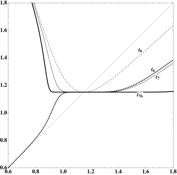
Figure 7: $f(x)=x^{11}+4\,x^{2}-10$. Comparison of results of $t_{76}$ and other iterative functions.

$$\begin{array}[]{| c || c | c| c | c| }\hline\cr t_{i}&t_{0}&t_{6}&t_{7}&t_{76}\\ \hline\cr s&0.5&5.3&7.6&2410.6\\ \hline\cr\end{array}$$

Table 8: $x_{0}=2$ (Example 4.4). Comparing the number of significant digits after 3 iterations.

Remark 4.1

Its is well-known that in the case of superlinear convergence the error of the $k$-th iterate $e_{k}=z-x_{k}$ can be well approximated by the difference $x_{k+1}-x_{k}$. For example, the number $s$ of significant digits, displayed in the second row of the Table 8 is in agreement with the following computations, when 4 iterations of $t_{76}$ are carried out, starting with $x_{0}=2$:

$$\begin{array}[]{ll}x_{1}=t_{76}(x_{0})&\Longrightarrow e_{0}\simeq x_{1}-x_{0}\simeq-0.799781\\ x_{2}=t_{76}(x_{1})&\Longrightarrow e_{1}\simeq x_{2}-x_{1}\simeq-0.0491500\\ x_{3}=t_{76}(x_{2})&\Longrightarrow e_{2}\simeq x_{3}-x_{2}\simeq-2.50444\times 10^{-44}\\ x_{4}=t_{76}(x_{2})&\Longrightarrow e_{3}\simeq x_{4}-x_{3}\simeq-2.75873\times 10^{-2411}\\ \end{array}$$

5 Conclusions

In the present article we have introduced a class of iterative methods for the numerical approximation of roots of nonlinear real functions. Our main goal is to propose a recursive algorithm to construct new iterative functions $t_{n}$, starting with the classical Newton’s method (to which corresponds the iterative function $t_{0}$), whose convergence order increases with $n$. For each $n$, our iterative function uses a Newton-Cotes closed quadrature rule with $n+1$ nodes. We have analysed the convergence of the introduced methods, and under certain restrictions on the regularity of the considered function, we have proved that each referred method has at least convergence order $n+2$. The presented numerical examples illustrate the performance of the discussed methods which can be easily extended to the case of nonlinear systems of equations. However, the analysis of the convergence in the multivariate case is left for another work. We also intend in the future to explore the application of the proposed methods to the solution of optimization problems.

References

- [1] A. Ben-Israel, Newton’s method with modified functions, Contemporary Math. 204, 1997, 39-50.
- [2] H. Brass and K. Petras, Quadrature Theory: The Theory of Numerical Integration on a Compact Interval, AMS, 2011.
- [3] A. Cordero and J. R. Torregrosa, Variants of Newton’s method for functions of several variables, Appl. Math. Comput. 183, 2006,199-208.
- [4] G. Dahlquist and Å. Björck, Numerical Methods in Scientific Computing, Volume I, SIAM, Philadelphia, 2008.
- [5] J. E. Dennis and J. J. Moré, A characterization of superlinear convergence and its application to quasi-Newton methods, Mat. Comput., 28, 549-560, 1974.
- [6] M. Frontini and E. Sormani, Third order methods for quadrature formulae for solving systems of nonlinear equations, Appl. Math. Comput. 149, 2004, 771-782.
- [7] W. Gautschi, Numerical Analysis, An Introduction, Birkhäuser, Boston, 1997.
- [8] E. Isaacson and H. B. Keller, Analysis of Numerical Methods, John Wiley and Sons, New York, 1966.
- [9] M. M. Graça, Removing multiplicities in by double newtonization, Appl. Math. Comput. 215(2), 2009, 562-572.
- [10] M. M. Graça and M. E. Sousa-Dias, A unified framework for the computation of polynomial quadrature weights and errors, available at arXiv:1203.4795v2, March, 2012.
- [11] M. A. Hafiz and M. M. Bahgat, An efficient two-step iterative method for solving systems of nonlinear equations, J. Math. Res., Vol 4., No. 4, 2012.
- [12] E. Halley, A new exact and easy method for finding the roots of equations generally and without any previous reduction, Phil. Roy. Soc. London 18, 1964, 136-147.
- [13] C. T. Kelley, Iterative Methods for Linear and Nonlinear Equations, SIAM, Philadelphia, 1995.
- [14] V. I. Krylov, Approximate Calculation of Integrals, Dover, New York, 2005.
- [15] A. Melman, Geometry and convergence of Halley’s method, SIAM Rev. 39 (4), 1997, 728-735.
- [16] N. A. Mir, N. Rafiq and N. Yasmin, Quadrature based three-step iterative method for nonlinear equations, Gen. Math, Vol. 18, No. 4, 2010, 31-42.
- [17] W. C. Rheinboldt, Methods for Solving Systems of Nonlinear Equations, SIAM, 2nd ed., Philadelphia, 1998.
- [18] R. Thukral, New Sixteenth-Order Derivative-Free Methods for Solving Nonlinear Equations, Amer. J. Comput. and Appl. Math. 2 (3), 2012, 112-118.
- [19] J. F. Traub, Iterative Methods for the Solution of Equations, Prentice-Hall, Englewood Cliffs, 1964.
- [20] N. Ujević, A method for solving nonlinear equations, Appl. Math. Comput. 174, 2006, 1416-1426.
- [21] L. Yau and A. Ben-Israel, The Newton and Halley Methods for Complex Roots, Amer. Math. Monthly 105, 1998, 806-818.
- [22] S. Weerakoom and T. G. I. Fernando, A Variant of Newton’s Method with Accelerated Third-Order Convergence, Appl. Math. Lett. 13, 2000, 87-93.
- [23] S. Wolfram, The Mathematica Book, Wolfram Media, fifth ed., 2003.