A Gyrokinetic 1D Scrape-Off Layer Model of an ELM Heat Pulse

Abstract

An electrostatic gyrokinetic-based model is applied to simulate parallel plasma transport in the scrape-off layer to a divertor plate. The authors focus on a test problem that has been studied previously, using parameters chosen to model a heat pulse driven by an edge-localized mode (ELM) in JET. Previous work has used direct particle-in-cell equations with full dynamics, or Vlasov or fluid equations with only parallel dynamics. With the use of the gyrokinetic quasineutrality equation and logical sheath boundary conditions, spatial and temporal resolution requirements are no longer set by the electron Debye length and plasma frequency, respectively. This test problem also helps illustrate some of the physics contained in the Hamiltonian form of the gyrokinetic equations and some of the numerical challenges in developing an edge gyrokinetic code.

I Introduction

One of the major issues for ITER and subsequent higher-power tokamaks is the power load on plasma-facing components (PFCs) from energy expelled into the scrape-off layer (SOL) by edge-localized modes. Excessive total and peak power loads from ELM heat pulses can cause the erosion or melting of divertor targets. Large Type I ELMs can also result in erosion to the main chamber wall and the release of impurities into the core plasma.Pitts et al. (2005) Suppressing ELMs or mitigating the damage they cause to PFCs is crucial for the viability of reactor-scale tokamaks. An accurate prediction of heat fluxes on future devices is important for the development of mitigation concepts.

Numerical simulations of heat pulse propagation can provide useful information about the time dependence of the power load on divertor targets. A test case involving the propagation of a heat pulse from an ELM along a scrape-off layer to a divertor target plate has been used as a benchmark in recent literature. This problem was first studied using a particle-in-cell (PIC) code and was demonstrated to have good agreement with experiment.Pitts et al. (2007) A Vlasov-Poisson model was later developed to study this problem.Manfredi, Hirstoaga, and Devaux (2011) A benchmark of fluid, Vlasov, and PIC approaches to this problem was recently described in Ref. [Havlíčková et al., 2012]. An implementation of this test case in BOUT++ was used to compare non-local and diffusive heat flux models for SOL modeling.Omotani and Dudson (2013) With the exception of initial conditions, the parameters we have adopted for our simulations are described in Ref. [Havlíčková et al., 2012]. This test case involves just one spatial dimension (along the field line), treating an ELM as an intense source near the midplane without trying to directly calculate the magnetohydrodynamic instability and reconnection processes that drive the ELM. Nevertheless, this is a useful problem for testing codes and understanding some of the physics involved in parallel propagation and divertor heat fluxes.

Unlike previous approaches, we have developed and studied gyrokinetic-based models with sheath boundary conditions using fully kinetic electrons or by assuming a Boltzmann response for the electrons. As is often done in gyrokinetics (unless looking at very small electron-scale turbulence where quasineutrality does not hold), a gyrokinetic quasineutrality equation (which includes a polarization-shielding term) is used, so the Debye length does not need to be resolved. To handle the sheath, logical sheath boundary conditionsParker et al. (1993) are used, which maintain zero net current to the wall at each time step. Although our simulations are one-dimensional, perpendicular effects can be incorporated by assuming axisymmetry. In an axisymmetric system, poloidal gradients have components that are both parallel and perpendicular to the magnetic field. The perpendicular ion polarization dynamics then enter the field equation by accounting for the finite pitch of the magnetic field.

An advantage of the models we have developed is their low computational cost. Earlier kinetic models have been described as computationally intensive Pitts et al. (2007) due to restrictions in the time step to $\sim\omega_{pe}^{-1}$ and in the spatial resolution to $\sim\lambda_{De}$. (A 1D Vlasov model using an asymptotic-preserving implicit numerical scheme described in Ref. [Manfredi, Hirstoaga, and Devaux, 2011] was able to relax these restrictions somewhat for this problem, using $\Delta x\sim 2\lambda_{De}$ and $\Delta t\sim 4/\omega_{pe}$ because their simulation still included the sheath directly.) By using a gyrokinetic-based model and logical sheath boundary conditions, our code can use grid sizes and time steps that are several orders of magnitude larger than this. It is fully explicit at present, though one could consider extending it to use implicit methods (such as in Ref. [Manfredi, Hirstoaga, and Devaux, 2011]) in the future. While fluid models have their own merits, they miss some kinetic effects, including the effect of hot tail electrons on the heat flux on the divertor plate and the subsequent rise of sheath potential.

We have implemented our models in Gkeyll, a code employing discontinuous Galerkin (DG) methods that is being developed for several applications, including solving gyrokinetic equations in the edge region. Although Gkeyll is currently being extended to have 5D capability, we focus on $1x$+$1v$ $(v_{\parallel})$ simulations in this paper for comparison with the similar $1x$+$1v$ Vlasov code in Ref. [Havlíčková et al., 2012].

An explicit third-order strong-stability-preserving Runge-Kutta algorithm is used to advance the system in time.Gottlieb, Shu, and Tadmor (2001) A review of the Runge-Kutta DG algorithm is given by Cockburn and Shu.Cockburn and Shu (2001) Our modifications to the basic DG scheme are applicable to a general class of Hamiltonian evolution equations and conserve energy exactly even when upwind fluxes are used (in addition to conserving particles exactly). These details will be described in a future publication.

Gyrokinetic codes that are fairly comprehensive (including general magnetic fluctuations to varying degrees) have been developedDorland et al. (2000); Kotschenreuther, Rewoldt, and Tang (1995); Jenko et al. (2000); Candy and Waltz (2003a, b); Parker et al. (2004); Peeters et al. (2009); Bottino et al. (2010); Maeyama et al. (2013) for the main core region of fusion devices and have been fairly successful in explaining core turbulence in many parameter regimes. However, extensions are needed to handle the additional complexities of the edge region ($r/a>0.9$), such as open and closed field lines, plasma-wall interactions, large amplitude fluctuations, and electromagnetic fluctuations near the beta limit. The test problem studied here is a useful first step in testing gyrokinetic algorithms for the edge region. Such a code could also be used to simulate linear devices (such as LAPDUmansky et al. (2011) and VinetaKervalishvili et al. (2006)) used for studying fundamental plasma physics phenomena.

Section II describes an electrostatic 1D gyrokinetic-based model with a modification to the ion-polarization term to set a minimum value for the wave number. Numerical implementation details and the logical sheath boundary condition are described in Section III. Results from numerical simulations and specific initial conditions are presented in Section IV.

II Electrostatic 1D gyrokinetic model with kinetic electrons

In this paper, we focus on the long-wavelength-drift-kinetic limit of gyrokinetics and ignore finite-Larmor-radius effects for simplicity. Polarization effects are kept in the gyrokinetic Poisson equation, and the model has the general form of gyrokinetics and can be extended to include full gyroaveraging in the future.

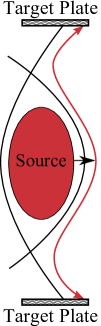
(a)

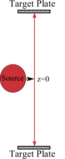
(b)

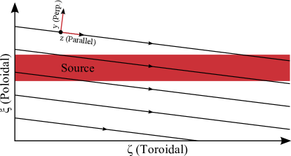
(c)

Figure 1: Illustration of the geometry used in the ELM SOL heat pulse test problem. The scrape-off layer region in the poloidal cross section LABEL:sub@fig:geoA is treated as straight LABEL:sub@fig:geoB in this test, with the ELM represented by an intense source near the midplane region. The time history of the resulting heat flux to the target plate is calculated in the simulation. The side view LABEL:sub@fig:geoC illustrates that although there is no toroidal variation in this axisymmetric problem, poloidal variations lead to both parallel and perpendicular gradient components.

The geometry used in the ELM SOL heat pulse test problem is illustrated in Fig. 1. The Vlasov and fluid codes used in Ref. [Havlíčková et al., 2012] consider only the parallel dynamics, while the 1$x$-3$v$ PIC code used in Ref. [Havlíčková et al., 2012] includes full orbit (not gyro-averaged) particle dynamics in an axiysmmetric system and so would automatically include polarization effects on time scales longer than an ion gyroperiod.

The gyrokinetic equation can be written as a Hamiltonian evolution equation for species $s$ of a plasma

$$\frac{\partial f_{s}}{\partial t}=\{H_{s},f_{s}\},$$ (1)

where $H_{s}=p_{\parallel}^{2}/2m_{s}+q_{s}\phi-m_{s}V_{E}^{2}/2$ is the Hamiltonian for the 1D electrostatic case considered here, $p_{\parallel}=m_{s}v_{\parallel}$ is the parallel momentum, and $\{f,g\}=(\partial f/\partial z)(\partial g/\partial p_{\parallel})-(\partial f/\partial p_{\parallel})(\partial f/\partial z)$ is the Poisson bracket operator for any two functions $f$ and $g$. The potential is determined by a gyrokinetic Poisson equation (in the long-wavelength quasineutral limit):

$$-\partial_{\perp}\left(\epsilon_{\perp}\partial_{\perp}\phi\right)=\frac{\sigma_{g}}{\epsilon_{0}}=\frac{1}{\epsilon_{0}}\sum_{s}q_{s}\int dv_{\parallel}\,f_{s}.$$ (2)

Here, $\sigma_{g}$ is the guiding-center charge density, while the left-hand side is the negative of the polarization contribution to the density, where the plasma perpendicular dielectric is

$$\epsilon_{\perp}=\frac{c^{2}}{v_{A}^{2}}=\sum_{s}\frac{n_{s}m_{s}}{\epsilon_{0}B^{2}}.$$ (3)

The ion polarization dominates this term, but a sum over all species has been included for generality.

In the Hamiltonian, $V_{E}=-(1/B)\partial_{\perp}\phi$ is the $\boldsymbol{E}\times\boldsymbol{B}$ drift in the radial direction (out of the plane in Fig. 1c). Since there is no variation in the radial direction, there is no explicit $\boldsymbol{V}_{E}\cdot\nabla$ term, and $V_{E}$ only enters through the second-order contribution to the Hamiltonian, $-mV_{E}^{2}/2$. Ref. [Krommes, 2013, 2012] provide some physical interpretations of this term, and Ref. [Krommes, 2013] gives a derivation of it in the cold-ion limit.

The conserved energy is given by

$$W_{\rm tot} =\int dz\sum_{s}\int dv_{\parallel}\,f_{s}H_{s}$$

$$=W_{K}+\int dz\,\sigma_{g}\phi-\frac{1}{2}\int dz\,\rho V_{E}^{2},$$ (4)

where $W_{K}=\int dz\sum_{s}\int dv_{\parallel}\,f_{s}m_{s}v_{\parallel}^{2}/2$ is the kinetic energy, and $\rho$ is the total mass density. Using the gyrokinetic Poisson equation (2) to substitute for $\sigma_{g}$ in this equation and doing an integration by parts (with a global neutrality condition $\int dz\sigma_{g}=0$ so boundary terms vanish), one finds that the total conserved energy can be written as

$$W_{\rm tot} =\frac{1}{2}\int dz\sum_{s}\int dv_{\parallel}\,f_{s}\left(m_{s}v_{\parallel}^{2}+m_{s}V_{E}^{2}\right)$$

$$=W_{K}+\frac{1}{2}\int dz\,\rho V_{E}^{2}.$$ (5)

To verify energy conservation, first note that $\int dz\int dv_{\parallel}H_{s}\partial f_{s}/\partial t=0$ by multiplying the gyrokinetic equation (1) by the Hamiltonian and integrating over all of phase-space. (Here, periodic boundary conditions are used for simplicity; there are of course losses to the wall in a bounded system.) The rate of change of the total conserved energy is then written as

$$\frac{dW_{\rm tot}}{dt} =\int dz\sum_{s}\int dv_{\parallel}\,f_{s}\left(q_{s}\frac{\partial\phi}{\partial t}-\frac{m_{s}}{2}\frac{\partial V_{E}^{2}}{\partial t}\right)$$

$$=\int dz\,\left(\sigma_{g}\frac{\partial\phi}{\partial t}-\frac{1}{2}\sum_{s}n_{s}m_{s}\frac{\partial V_{E}^{2}}{\partial t}\right).$$ (6)

Using the gyrokinetic Poisson equation (2) to substitute for $\sigma_{g}$ and integrating by parts, one finds that these two terms cancel, so $dW_{\rm tot}/dt=0$. Note that the small second-order Hamiltonian term $H_{2}=-(m/2)V_{E}^{2}$ was needed to get exact energy conservation. (In many circumstances, the $\boldsymbol{E}\times\boldsymbol{B}$ energy $mV_{E}^{2}$ is only a very small correction to the parallel kinetic energy $mv_{\parallel}^{2}/2$, but it is still assuring to know that exact energy conservation is possible.) This automatically occurs in the Lagrangian field theory approach to full-$F$ gyrokineticsSugama (2000); Brizard (2000); Krommes (2012), in which the gyrokinetic Poisson equation results from a functional derivative of the action with respect to the potential $\phi$, so a term that is linear in $\phi$ in the gyrokinetic Poisson equation comes from a term that is quadratic in $\phi$ in the Hamiltonian.

II.1 Electrostatic model with a modified ion polarization term

One can obtain a wave dispersion relation by linearizing Eqs. (1) and (2) and Fourier transforming in time and space. With the additional assumption that $q_{e}=-q_{i}$ and neglecting ion perturbations (except for the ion polarization density), one has

$$k_{\perp}^{2}\rho_{s}^{2}+\left[1+\xi Z\left(\xi\right)\right] =0.$$ (7)

Here, $\rho_{s}^{2}=T_{e}/(m_{i}\Omega_{ci}^{2})$, $\xi=\omega/(\sqrt{2}k_{\parallel}v_{\rm te})$, $v_{\rm te}=\sqrt{T_{e}/m_{e}}$, and $Z(\xi)=\pi^{-1/2}\int dt\exp(-t^{2})/(t-\xi)$ [or the analytic continuation of this for ${\rm Im}(\xi)\leq 0$] is the plasma dispersion function. In the limit $\xi\gg 1$, the solution to the dispersion relation is a wave with frequency

$$\omega_{H} =\frac{k_{\parallel}v_{\rm te}}{|k_{\perp}|\rho_{s}}.$$ (8)

For $k_{\perp}\rho_{s}\ll 1$, this is a very high-frequency wave that must be handled carefully to remain numerically stable. Note that this wave does not affect parallel transport in the SOL because the main heat pulse propagates at the ion sound speed, and this wave is even faster than the electrons for $k_{\perp}\rho_{s}\ll 1$.

This wave is the electrostatic limit of the shear Alfvén wave,Lee (1987); Belli and Hammett (2005) which lies in the regime of inertial Alfvén waves.Lysak and Lotko (1996); Vincena, Gekelman, and Maggs (2004) The difficulties introduced by such a wave could be eased by including magnetic perturbations from $A_{\parallel}$, in which case the dispersion relation (in the fluid electron regime $\xi\gg 1$) becomesBelli and Hammett (2005) $\omega^{2}=k_{\parallel}^{2}v_{\rm te}^{2}/(\hat{\beta}_{e}+k_{\perp}^{2}\rho_{s}^{2})$, where $\hat{\beta}_{e}=(\beta_{e}/2)(m_{i}/m_{e})$ and $\beta_{e}=2\mu_{0}n_{e}T_{e}/B^{2}$. In the electrostatic limit $\hat{\beta}_{e}=0$, we recover Eq. (8), but retaining a finite $\hat{\beta}_{e}$ would set a maximum frequency at low $k_{\perp}$ of $\omega=k_{\parallel}v_{\rm te}/\hat{\beta}_{e}^{1/2}=k_{\parallel}v_{A}$, where $v_{A}$ is the Alfvén velocity, avoiding the $k_{\perp}\rho_{s}\rightarrow 0$ singularity of the electrostatic case. (We shall defer further discussion of magnetic fluctuations to a future paper, as that brings up another set of interesting numerical subtleties.)

For electrostatic simulations, a modified ion polarization term can be introduced to effectively set a minimum value for the perpendicular wave number $k_{\perp}$. This modification can be used to slow down the electrostatic shear Alfvén wave to make it more numerically tractable. (Even when magnetic fluctuations are included, one still might want to consider an option of introducing a long wavelength modification for numerical convenience or efficiency.)

When choosing how to select the minimum value for $k_{\perp}\rho_{s}$, it is useful to consider the set of $k_{\perp}$’s represented on the grid for particular simulation parameters. Consider an axisymmetric system (as in Fig. 1c) with constant $B/B_{\xi}$, where $B$ is the total magnetic field, and $B_{\xi}$ and $B_{\zeta}$ are the components of $\boldsymbol{B}$ in the poloidal and toroidal directions. It follows that $\partial_{\perp}=(B_{\zeta}/B_{\xi})\partial_{\parallel}$, so

$$k_{\perp,\mathrm{max}} =\frac{B_{\zeta}}{B_{\xi}}k_{\parallel,\mathrm{max}}.$$ (9)

The maximum parallel wavenumber can be estimated as $k_{\parallel,\mathrm{max}}\Delta z\sim\pi N_{nc}$, where $\Delta z$ is the width of a single cell in position space, and $N_{nc}$ is the total degrees of freedom per cell used in the finite element DG representation of the position coordinate.

Therefore, one has

$$k_{\perp,\mathrm{max}} =\frac{B_{\zeta}}{B_{\xi}}\frac{\pi N_{nc}}{\Delta z}.$$ (10)

In our simulations, $N_{nc}=3$ and $\Delta z=10$ m using $8$ cells in the spatial direction to represent an $80$ m parallel length. Assuming that $B_{\xi}/B=\sin(6^{\circ})$, one estimates that $k_{\perp,\mathrm{max}}\rho_{s}\approx 2.5\times 10^{-2}$ for 1.5 keV deuterium ions with $B=2$ T. Thus, the perpendicular wave wavenumbers represented by a typical grid are fairly small.

The general modified gyrokinetic Poisson equation we consider is of the form

$$-\partial_{\perp}(C_{\epsilon}\epsilon_{\perp}\partial_{\perp}\phi)+s_{\perp}(z,t)(\phi-\langle\phi\rangle)=\frac{\sigma_{g}(z)}{\epsilon_{0}},$$ (11)

where $s_{\perp}(z,t)=k^{2}_{\rm min}(z){\epsilon_{\perp}(z,t)}$ is a shielding factor (we allow $k_{\rm min}$ to depend on position but not on time in order to preserve energy conservation, as described below) and $\langle\phi\rangle$ is a dielectric-weighted flux-surface-averaged potential defined as

$$\langle\phi\rangle =\frac{\int dz\,s_{\perp}\phi}{\int dz\,s_{\perp}}.$$ (12)

The fixed coefficient $C_{\epsilon}$ is for generality, making it easier to consider various limits later.

The sound gyroradius is chosen to be defined by $\rho_{s}^{2}(z,t)=c_{s}^{2}(z,t)/\Omega_{ci}^{2}=T_{e}(z,t)/(m_{i}\Omega_{ci}^{2})$, using the mass and cyclotron frequency of a main ion species. A time-independent sound gyroradius (using a typical or initial value for the electron temperature $T_{e0}$) is defined by $\rho_{s0}^{2}(z)=c_{s0}^{2}(z)/\Omega_{ci}^{2}=T_{e0}(z)/(m_{i}\Omega_{ci}^{2})$. Note that the shielding factor can also be written as $s_{\perp}(z,t)=[k_{\rm min}(z)\rho_{s0}(z)]^{2}{\epsilon_{\perp}(z,t)}/\rho^{2}_{s0}(z)$.

For simplicity, $k_{\rm min}\rho_{s0}$ is chosen to be a constant independent of position. Its value should be small enough that the wave in Eq. (8) is high enough in frequency that it does not interact with other dynamics of interest, but not so high in frequency that it forces the explicit time step to be excessively small. For some of our simulations, we use $k_{\rm min}\rho_{s}=0.2$, which leads to only a 2% correction to the ion acoustic wave frequency $\omega=k_{\parallel}c_{s}/\sqrt{1+k_{\perp}^{2}\rho_{s}^{2}}$ at long wavelengths. Convergence can be checked by taking the limit $k_{\rm min}\rho_{s0}\rightarrow 0$.

As a simple limit, one can even set $C_{\epsilon}=0$ and keep just the $s_{\perp}$ term, which replaces the usual differential gyrokinetic Poisson equation with a simpler algebraic model. This approach should work fairly well for low frequency dynamics. The basic idea is that for long-wavelength ion-acoustic dynamics, the left-hand side of Eq. (11) is small, so the potential is primarily determined by the requirement that it adjust to keep the electron density on the right-hand side almost equal to the ion guiding center density. (At low frequencies, the electron density is close to a Boltzmann response, which depends on the potential.) In future work, one could consider using an implicit method, perhaps using the method here as a preconditioner. Alternatively, electromagnetic effects will slow down the high-frequency wave so that explicit methods may be sufficient.

The flux-surface-averaged potential $\langle\phi\rangle$ is subtracted off in Eq. (11) so that the model polarization term is gauge invariant like the usual polarization term. This choice is also related to our form of the logical sheath boundary condition, which assumes that the electron and ion guiding center fluxes to the wall are the same so that the net guiding center charge vanishes, $\int dz\,\sigma_{g}=0$. Just as the net guiding center charge vanishes, our model polarization charge density, $s_{\perp}(\phi-\langle\phi\rangle)$, also averages to zero. This approach neglects ion polarization losses to the wall, which is consistent in this model because integrating Eq. (2) over all space then gives $\partial_{\perp}\phi=0$ at the plasma edge. (One could consider future modifications to account for polarization drift losses to the wall, but the present model is found to agree fairly well with full-orbit PIC results.)

With this approach, it is also necessary to modify the Hamiltonian in order to preserve energy consistency with this modified gyrokinetic Poisson equation. The modified Hamiltonian is written in the form

$$H_{s}=\frac{1}{2}m_{s}v_{\parallel}^{2}+q_{s}(\phi-\langle\phi\rangle)-\frac{1}{2}m_{s}\hat{V}_{E}^{2},$$ (13)

where $\hat{V}_{E}^{2}$ is a modified $\boldsymbol{E}\times\boldsymbol{B}$ velocity that is chosen to conserve energy. The constant $\langle\phi\rangle$ term in $H_{s}$ has no effect on the gyrokinetic equation because only gradients of $\phi$ matter, but it simplifies the energy conservation calculation. The total energy is still $W_{\rm tot}=\int dz\sum_{s}\int dv_{\parallel}\,f_{s}H_{s}$, and its time derivative (neglecting boundary terms that are straightforward to evaluate) can be written as

$$\frac{dW_{\rm tot}}{dt} =\int dz\sum_{s}\int dv_{\parallel}\,f_{s}\frac{\partial H}{\partial t}$$

$$=\int dz\left(\sigma_{g}\frac{\partial}{\partial t}\left(\phi-\langle\phi\rangle\right)-\sum_{s}\frac{1}{2}n_{s}m_{s}\frac{\partial}{\partial t}\hat{V}_{E}^{2}\right).$$ (14)

Using the modified gyrokinetic Poisson equation (11) and integrating the first term by parts gives

$$\frac{dW_{\rm tot}}{dt} =\int dz\Bigg{(}\sum_{s}\frac{1}{2}n_{s}m_{s}C_{\epsilon}\frac{\partial}{\partial t}V_{E}^{2}$$

$$+\frac{\epsilon_{0}}{2}s_{\perp}\frac{\partial}{\partial t}(\phi-\langle\phi\rangle)^{2}-\sum_{s}\frac{1}{2}n_{s}m_{s}\frac{\partial}{\partial t}\hat{V}_{E}^{2}\Bigg{)},$$ (15)

so energy is conserved if one chooses

$$\hat{V}_{E}^{2} =C_{\epsilon}V_{E}^{2}+\frac{\epsilon_{0}s_{\perp}}{\sum_{s}n_{s}m_{s}}(\phi-\langle\phi\rangle)^{2}$$ (16)

and require that the coefficient $\epsilon_{0}s_{\perp}/(\sum_{s}n_{s}m_{s})$ be independent of time so that it comes outside of a time derivative. Using Eq. (3) and the definition of $s_{\perp}$ after Eq. (11), one sees that $\epsilon_{0}s_{\perp}/(\sum_{s}n_{s}m_{s})=k_{\rm min}^{2}(z)/B^{2}$, which is indeed independent of time because $k_{\rm min}$ was chosen not to have any time dependence.

In the limit that one uses only the algebraic model polarization term with $C_{\epsilon}=0$, one finds that

$$\hat{V}_{E}^{2}=(k_{\rm min}\rho_{s0})^{2}\left(\frac{e\delta\phi}{T_{e0}}\right)^{2}c_{s0}^{2},$$ (17)

where $\delta\phi=\phi-\langle\phi\rangle$. For $k_{\rm min}\rho_{s0}=0.2$ and $e\delta\phi/T_{e0}\sim 1$, this $\boldsymbol{E}\times\boldsymbol{B}$ energy could be order 4% of the total energy.

III Numerical implementation details

One detail of solving the modified gyrokinetic Poisson equation (11) is how to determine the flux-surface-averaged component, which is related to the boundary conditions. Consider the case in which $\epsilon_{\perp}=0$, and expand $\phi=\langle\phi\rangle+\delta\phi$. Then $\delta\phi$ is determined by the algebraic equation

$$s_{\perp}(z)\,\delta\phi(z)=\frac{\sigma_{g}(z)}{\epsilon_{0}}.$$ (18)

Imposing the boundary condition that the value of $\phi$ at the plasma edge be equal to the sheath potential gives $\phi(z_{R})=\phi_{s}=\langle\phi\rangle+\delta\phi(z_{R})$ (the left and right boundaries have been assumed to be symmetric here), which gives an additional equation to determine $\langle\phi\rangle$. The final expression is

$$\phi(z)=\delta\phi(z)-\delta\phi(z_{R})+\phi_{s}.$$ (19)

In order to maintain energy conservation, it is important that the algorithm preserve the numerical equivalent of certain steps in the analytic derivation. In our algorithm, based on Liu and Shu’s Liu and Shu (2000) algorithm for the incompressible Euler equation, $\phi$ must be obtained using continuous finite elements, although the charge density $\sigma_{g}$ is discontinuous in our Poisson equation.

To preserve the integrations involved in energy conservation, it is important to ensure that one can multiply Eq. (18) by the fluctuating potential, integrate over all space, and preserve

$$\int dz\,\delta\phi\,s_{\perp}\,\delta\phi=\frac{1}{\epsilon_{0}}\int dz\,\delta\phi\,\sigma_{g}.$$ (20)

This requirement ensures that a potential part of the energy on the right-hand side is exactly related to a field-like-energy on the left-hand side. This quantity will be preserved if one projects the modified Poisson equation onto all of the continuous basis functions $\psi_{j}$ that are used for $\phi$ (i.e., $\phi(z)=\sum_{j}\phi_{j}\psi_{j}(z)$) to ensure that

$$\langle\psi_{j}s_{\perp}\phi\rangle=\langle\psi_{j}\sigma_{g}\rangle.$$ (21)

For piecewise linear basis functions, this leads to a tri-diagonal equation for $\phi_{j}$ that has to be inverted to determine $\phi$. Because $s_{\perp}\propto n(z,t)$ varies in time, this will take a little bit of work, but as one goes to higher dimensions in velocity space, the Poisson solve (which is only in the lower-dimensional configuration space) will be a negligible fraction of the computational time.

III.1 Boundary Conditions

Gyrokinetics does not need to resolve the restrictive Debye length ($\sim\lambda_{De}$) or plasma frequency time scales ($\sim\omega_{pe}^{-1}$), so the sheath is usually not directly resolved. Instead, the effects of the sheath can be incorporated through the use of logical sheath boundary conditions.Parker et al. (1993) For a normal positive sheath, all incident ions flow into the wall, but incident electrons with energies below the sheath potential are reflected back into the domain such that there is zero net current into the wall. (For biased endplates or higher dimensional problems with non-insulating walls, one could consider more general boundary conditions that involve currents in and out of the wall at various places.) At the right boundary, for example, this condition is expressed as

$$\int_{0}^{\infty}dv\thinspace vf_{i}(z_{R},v,t) =\int_{v_{c}}^{\infty}dv\thinspace vf_{e}(z_{R},v,t),$$ (22)

where $z_{R}$ is the coordinate of the domain edge. The cutoff velocity $v_{c}>0$ is determined numerically through a search algorithm. The sheath potential is then determined using the relation $e\phi_{s}=m_{e}v_{c}^{2}/2$.

In order to reflect all electrons incident on the sheath with velocity in the range $0<v<v_{c}$, the electron distribution function in this range is copied into ghost cells according to

$$f_{e}(z_{R},-v,t) =f_{e}(z_{R},v,t),\quad 0<v<v_{c},$$ (23)

and $f_{e}(z_{R},-v,t)=0$ for $v>v_{c}$. This condition can also be written as $f_{e}(z_{R},-v,t)=f_{e}(z_{R},v,t)H(v_{c}-v)$ for $v>0$. This condition results in the reflection of electrons with velocity in the range $0<v<v_{c}$ back into the domain with the opposite velocity, while the electrons with energy sufficient to overcome the sheath potential will flow out of the system to the divertor plates.

The implementation of logical sheath boundary conditions needs a slight modification for use in a continuum code. Typically, the cutoff velocity will fall within a cell and not exactly on a cell edge. A direct projection of the discontinuous reflected distribution onto the basis functions used in a cell could lead to negative values of the distribution function at some velocities in the cell. Future work could consider methods of doing higher-order projections that incorporate positivity constraints, but for now we have used a simple scaling method, in which the entire distribution function inside the “cutoff cell” is copied into the ghost cell and then scaled by the fraction required to ensure that the electron flux at the domain edge equals the ion flux. For scaling the reflected distribution function in the cutoff cell on the right boundary, this fraction is

$$c =\frac{\int_{v_{j}-\Delta v/2}^{v_{c}}dv\,vf_{e}(z_{R},v,t)}{\int_{v_{j}-\Delta v/2}^{v_{j}+\Delta v/2}dv\,vf_{e}(z_{R},v,t)},$$ (24)

where $\Delta v$ is the cell width in velocity space, and $v_{j}$ denotes the center of the cell.

IV Simulation Results

The main parameters used for our simulations were described in Ref. [Havlíčková et al., 2012] and were chosen to model an ELM on the JET tokamak for a case in which the density and temperature at the top of the pedestal were $n_{\rm ped}=5\times 10^{19}$ m^-3 and $T_{\rm ped}=1.5$ keV. The ELM is modelled as an intense particle and heat source in the SOL that lasts for 200 $\mu$s, spread over a poloidal length of 2.6 m around the midplane (as described below) and a radial width in the SOL of 10 cm. The model SOL has a major radius of 3 m, and this source corresponds to a total ELM energy of about 0.4 MJ. The simulation domain has a length of $2L_{||}=80$ m, the length of a magnetic field line in the SOL, with a field line pitch of $6^{\circ}$. The kinetic equation with the source term on the right-hand side is

$$\frac{\partial f}{\partial t}-\{H,f\}=g(t)\,S(z)\,F_{M}\boldsymbol{(}v_{\parallel},T_{S}(t)\boldsymbol{)},$$ (25)

where $F_{M}\boldsymbol{(}v_{\parallel},T_{S}(t)\boldsymbol{)}$ is a unit Gaussian in variable $v_{\parallel}$ with a time-dependent temperature $T_{S}(t)$. The function $S(z)$ is the same for both particle species, and is represented as

$$S(z) =\begin{cases}S_{0}\cos\left(\frac{\pi z}{L_{s}}\right)&|z|<\frac{L_{s}}{2}\\ 0&\mathrm{else}\end{cases},$$ (26)

where $L_{s}=25$ m is length of the source along the magnetic field line. The value of $S_{0}$ was computed using the scalingHavlíčková et al. (2012)

$$S_{0}=A\,n_{ped}\,c_{s,ped}/L_{s},$$ (27)

where the constant of proportionality $A$ was chosen to be $1.2\sqrt{2}\approx 1.7$ for comparison with Ref. [Havlíčková et al., 2012]. In our simulations, $S_{0}\approx 9.066\times 10^{23}$ m^-3 s^-1.

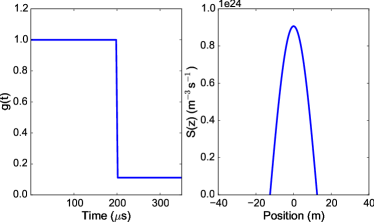
Figure 2: Spatial and temporal profiles of the source term on the right-hand side of Eq. (25).

The function $g(t)$ in Eq. (25) is used to model the time-dependence of the particle source:

$$g(t) =\begin{cases}1&0<t<200\,\mu\mathrm{s}\\ 1/9&t>200\,\mu\mathrm{s}\end{cases}.$$ (28)

The post-ELM source also has reduced electron and ion temperature, represented by the $T_{S}(t)$ parameter in the Maxwellian term $F_{M}$ in Eq. (25), which has the value $1.5$ keV from $0<t<200$ $\mu$s for both ions and electrons. The electron temperature for $t>200$ $\mu$s is 210 eV, and the ion temperature is reduced to 260 eV. The end time for the simulation is $t=350$ $\mu$s.

We performed our simulations using second-order serendipity basis functions Arnold and Awanou (2011) on a grid with 8 cells in the spatial direction and 32 cells in the velocity direction. (In 1D, second-order basis functions correspond to piecewise parabolic basis functions, or 3 degrees of freedom within each cell.) The case with kinetic electrons and ions takes only about three minutes to run on a standard laptop, although we have not yet extensively optimized our code.

IV.1 Initial Conditions

In previous papers that looked at this problem, the codes were typically run for a while with the same weak source that would be used in the post-ELM phase to reach a quasi-steady state before the intense ELM source was turned on. The authors found that the final results were not very sensitive to the duration of the pre-ELM phase or the initial conditions used for it. However, there is formally no normal steady state for this problem in the collisionless limit (low energy particles build up over time without collisions). To remove a possible source of ambiguity for future benchmarking, here we specify more precise initial conditions chosen to approximately match initial conditions at the beginning of the ELM phase used in previous work.

We model the initial electron distribution function as

$$f_{e0}(z,v_{\parallel}) =n_{e0}(z)F_{M}(v_{\parallel},T_{e0}),$$ (29)

with $T_{e0}=75$ eV. The electron density profile (in $10^{19}$ m^-3) is defined as

$$n_{e0}(z) =0.7+0.3\left(1-\left|\frac{z}{L_{\parallel}}\right|\right)$$

$$\qquad{}+0.5\cos\left(\frac{\pi z}{L_{s}}\right)H\left(\frac{L_{s}}{2}-|z|\right).$$ (30)

The initial ion distribution function is modeled as

$$f_{i0}(z,v_{\parallel})=\begin{cases}F_{L}&z<-\frac{L_{s}}{2}\\ \begin{aligned} &\Bigg{[}\left(\frac{1}{2}-\frac{z}{L_{s}}\right)F_{L}\\ &\quad{}+\left(\frac{1}{2}+\frac{z}{L_{s}}\right)F_{R}\Bigg{]}\end{aligned}&-\frac{L_{s}}{2}<z<\frac{L_{s}}{2}\\ F_{R}&z>\frac{L_{s}}{2}\end{cases}.$$ (31)

Here, $F_{L}$ and $F_{R}$ are left and right half-Maxwellians defined as

$$F_{R}(z,v_{\parallel};T_{i0}) =\hat{n}(z)F_{M}(v_{\parallel},T_{i0})H(v_{\parallel}),$$ (32)

$$F_{L}(z,v_{\parallel};T_{i0}) =\hat{n}(z)F_{M}(v_{\parallel},T_{i0})H(-v_{\parallel}),$$ (33)

where $\hat{n}(z)=2n_{i0}(z)$, $H$ is the Heaviside step function, and the initial ion temperature profile (in eV) is defined as

$$T_{i0}(z) =100+45\left(1-\left|\frac{z}{L_{\parallel}}\right|\right)$$

$$\qquad{}+30\cos\left(\frac{\pi z}{L_{s}}\right)H\left(\frac{L_{s}}{2}-|z|\right).$$ (34)

The expressions for the $n_{e0}$ and $T_{i0}$ profiles were chosen to approximate those described in private communication with the author of Ref. [Havlíčková et al., 2012],Havlíčková (2012) which were originally obtained from simulations that had run for a while with a weaker source to achieve a quasi-steady state before the strong ELM source was turned on, as described at the beginning of this subsection.

Given an initial electron density profile, we then calculate an initial ion guiding center density profile to minimize the excitation of high-frequency kinetic Alfvén waves. We do this by choosing the initial ion guiding-center density $n_{i}(z)$ so that it gives a potential $\phi(z)$ that results in the electron density’s being consistent with a Boltzmann equilibrium, i.e., the electrons are initially in parallel force balance and do not excite high-frequency kinetic Alfvén waves. A Boltzmann electron response is

$$n_{e}(z) =C\exp\left(\frac{e\phi(z)}{T_{e}}\right).$$ (35)

Taking the log of the above equation and then an $n_{e}$-weighted average, one has

$$\langle\log n_{e}\rangle_{n_{e}} =\log C+\frac{e\langle\phi\rangle_{n_{e}}}{T_{e0}},$$ (36)

where $T_{e}$ has been assumed to be a constant $T_{e0}$.

Note that one is free to add an arbitrary constant to $\phi$ since only gradients of $\phi$ affect the dynamics. Choosing the additional constraint that $\langle\phi\rangle_{n_{e}}=0$, one can express the constant $C$ in terms of $n_{e}$. (This convention for $\langle\phi\rangle_{n_{e}}$ is only for convenience, as any constant can be added to $\phi$ in the plasma interior without affecting the results. After the first time step, the sheath boundary condition will be imposed, which will give a non-zero value for the average potential.)

One then has the following equation for $\phi$:

$$\frac{e\phi}{T_{e0}} =\log n_{e}-\langle\log n_{e}\rangle_{n_{e}}.$$ (37)

This $\phi$ can be used with the gyrokinetic Poisson equation to solve for $n_{i}(z)$ by iteration. With a small $m_{e}/m_{i}$ ratio, the gyrokinetic Possion equation can be written as

$$n_{i}(z)\left(1-k_{\perp}^{2}\rho_{s0}^{2}\frac{e(\phi-\langle\phi\rangle_{n_{i}})}{T_{e0}}\right) =n_{e}(z),$$ (38)

where with the small $m_{e}/m_{i}$ ratio approximation, the dielectric-weighted average is equivalent to an ion density-weighted average. The left-hand side of this equation is a nonlinear function of $n_{i}$ (because it appears as a leading coefficient and in the density-weighted average $\langle\phi\rangle_{n_{i}}$), which is solved for by using iteration:

$$n_{i}^{j+1}(z) =\frac{n_{e}(z)}{1-k_{\perp}^{2}\rho_{s0}^{2}\frac{e}{T_{e0}}\left(\phi-\langle\phi\rangle_{n_{i}^{j}}\right)}.$$ (39)

Note that the the averaged $\phi$ on the right-hand side is weighted by $n_{i}^{j}$, the previous iteration’s ion density. Convergence can be improved by adding a constant to $n_{i}(z)$ each iteration to enforce global neutrality $\langle n_{i}\rangle=\langle n_{e}\rangle$. In our tests, the initial ion density profile was calculated to $10^{-15}$ relative error in five iterations.

IV.2 Divertor heat flux with drift-kinetic electrons

Figure 3: Parallel heat flux at the divertor plate vs. time with drift-kinetic electrons. The electron and ion thermal transit times $\tau_{e}$ and $\tau_{i}$ are indicated by the vertical dashed lines.

Figure 3 shows the parallel heat flux on the target plate vs. time using the 1D electrostatic model with a fixed $k_{\perp}\rho_{s0}=0.2$. A rapid response in the electron heat flux is observed at early times, on the order of the electron transit timescale $\tau_{e}\sim L_{\parallel}/v_{\rm te,ped}\approx 2.46$ $\mu$s. This response is due to fast electrons reaching the target plate, which initially cause a modest rise in the electron heat flux from $t\sim 1$ $\mu$s to $t\sim 1.5$ $\mu$s. This build-up of fast electrons result in a rise in the sheath potential at $t\sim 1.5$ $\mu$s, which causes a modest rise in the ion heat flux and a modest drop in the electron heat flux until the arrival of the bulk ion heat flux at a later time. We did a scan in $k_{\perp}^{2}\rho_{s0}^{2}$ over a factor of 20 (from $k_{\perp}^{2}\rho_{s0}^{2}=0.04$ to 0.1) and found only a few percent variation in the resulting plot of heat flux vs. time, verifying that the results are not sensitive to the exact value of this parameter (as long as it is small).

As pointed out in a recent invited talk,Leonard (2014) one of the original motivations for calculations of this kind (such as Ref. [Pitts et al., 2007]) was a concern that the fast parallel thermal transport of electrons would cause a very large heat flux to arrive at the divertor plates on the electron transit time scale. Our results confirm the previous calculations that found that although there is a modest rise in the heat flux on the electron transit time scale, the sheath potential (and the potential variation along the field line) increases to confine most of the electrons so that the bulk of the ELM energy arrives at the target plate only on the slower ion time scale. (Nevertheless, even this ELM power is so large that erosion of solid target plates is a concern, and methods of mitigating or avoiding ELMs are being studied.)

The bulk of the ELM energy is carried by the ions, which arrive at the target plate on the order of the ion thermal transit timescale, $\tau_{i}\sim L_{\parallel}/v_{\rm ti}\approx 149$ $\mu$s. The reduction of source strength and temperature after $200$ $\mu$s results in the abrupt drop seen in the electron heat flux.

The parallel heat flux (parallel to the magnetic field) on the right target plate for each species is calculated as

$$Q_{s} =\frac{1}{2}m_{s}\int_{v_{c,s}}^{\infty}dv\,f_{s}\,v^{3}+(T_{\perp}+q_{s}\phi_{s})\int_{v_{c,s}}^{\infty}dv\,f_{s}\,v,$$ (40)

where $v_{c,s}=\sqrt{\mathrm{max}(-2q_{s}\phi_{s}/m_{s},0)}$ accounts for the reflection of electrons by the sheath. The $q_{s}\phi_{s}$ term in the second integral models the acceleration of ions and deceleration of electrons as they pass through the sheath to the divertor plate, a region that is not resolved in our models. We have assumed that each species has a constant perpendicular temperature $T_{\perp}=T_{ped}$ for comparison with the 1D Vlasov results in Ref. [Havlíčková et al., 2012]. Note that the pitch angle of the magnetic field is not factored into this measure of heat flux on the target plate. The heat flux normal to the target plate is $Q_{s,n}=Q_{s}\sin(\theta)$, where $\theta$ is the (usually very small) angle between the magnetic field and the surface.

Figure 3 agrees well with the $1x$+$1v$ Vlasov and full $1x$+$3v$ PIC results in Ref. [Havlíčková et al., 2012], providing a useful benchmark for these codes and supporting the accuracy of the sheath boundary conditions and the gyrokinetic-based model used here. (The small differences between our $1x$+$1v$ results, the Vlasov results, and the PIC results are probably due to small differences in initial conditions and the inclusion of collisions in the PIC code.)

IV.3 Divertor heat flux with Boltzmann electron model

We have also investigated a model that includes the effect of kinetic ions but assumes a Boltzmann response for the electrons. Specifically, the electron density takes the form

$$n_{e}(z) =n_{e}(z_{R})\exp\left(\frac{e(\phi-\phi_{s})}{T_{e}}\right),$$ (41)

where $n_{e}(z_{R})$ is the electron density evaluated at the domain edge. This expression can be inverted to give another algebraic equation to determine the potential, similar to the electrostatic gyrokinetic model with a fixed $k_{\perp}\rho_{s0}$. Since the time step is set by the ions, these simulations have an execution time a factor of $\sim\sqrt{m_{i}/m_{e}}$ faster than the gyrokinetic simulation. This property makes the Boltzmann electron model useful as a test case for code development and debugging.

The sheath potential $\phi_{s}$ can be determined by assuming that $f_{e}$ at the target plate is a Maxwellian with temperature $T_{e}$. By using logical sheath boundary conditions and quasineutrality,

$$\phi_{s} =-\frac{T_{e}}{e}\log\left(\frac{\sqrt{2\pi}\Gamma_{i}}{n_{i}v_{\rm te}}\right),$$ (42)

where $\Gamma_{i}$ is the outward ion flux, and all quantities are evaluated at the domain edge. For simplicity, we selected $T_{e}$ in our simulations to be the field-line-averaged value of the ion temperature $T_{i}(z)$, but more accurate models for $T_{e}$ could be used.

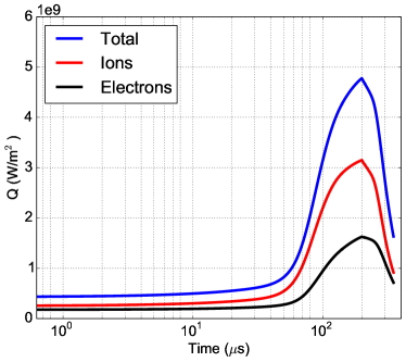
Figure 4: Parallel heat flux at the divertor plate vs. time from the Boltzmann electron model.

Figure 4 shows the parallel heat flux on the target plate vs. time using Boltzmann electrons. As expected, kinetic electron effects present in Fig. 3 are not resolved by this model. When compared to a simulation using kinetic electrons, the main heat flux at $t\sim 100-200$ $\mu$s is predicted fairly well by the Boltzmann electron model.

The expression for the electron parallel heat flux on the target plate is calculated as

$$Q_{e} =\frac{1}{2}m_{e}\int_{v_{c}}^{\infty}dv\,f_{e}\,v^{3}+(T_{\perp}-e\phi_{s})\int_{v_{c}}^{\infty}dv\,f_{e}\,v$$

$$=(T_{e}+T_{\perp})\int_{0}^{\infty}dv\,f_{i}\,v.$$ (43)

V Conclusions

We have used a gyrokinetic-based model to simulate the propagation of a heat pulse along a scrape-off layer to a divertor target plate. We have described a modification to the ion polarization term to slow down the electrostatic shear Alfvén wave.

Our main results include the demonstration that this gyrokinetic-based model with logical sheath boundary conditions is able to agree well with Vlasov and full-orbit (non-gyrokinetic) PIC simulations, without needing to resolve the Debye length or plasma frequency. This simplification allows the spatial resolution to be several orders of magnitude coarser than the electron Debye length (and the time step several orders of magnitude larger than the plasma period) and thus leads to a much faster calculation. Our results also confirm previous work that the electrostatic potential in this problem varies to confine most of the electrons on the same time scale as the ions, so the main ELM heat deposition occurs on the slower ion transit time scale.

Additionally, we have described a model using Boltzmann electrons that is useful for code development and debugging. This model does not include kinetic electron effects but runs much faster than simulations with kinetic electrons and ions.

Although this paper focuses on electrostatic simulations, we have also extended our simulations to include magnetic fluctuations. These extensions involve a number of interesting and subtle physics and algorithm issues that will be described in a future paper.

Since we have assumed only a single $k_{\perp}$ mode in our simulations to limit the high frequency of the electrostatic shear Alfvén wave, future work can include allowing a spectrum of $k_{\perp}$ modes. For 1D electromagnetic simulations, this modification requires inverting the $\nabla_{\perp}^{2}$ operators that appear in the gyrokinetic Poisson equation and Ampere’s law. We defer further discussion of this to a future paper because including a magnetic component to the fluctuations will be important when a spectrum of very low $k_{\perp}$ modes is kept in order to limit on the frequency of the shear Alfvén wave at low $k_{\perp}$.

Future work on these models can also include extensions to higher spatial and velocity dimensions. An axisymmetric 2D model can use a specified diffusion coefficient to model radial transport in the SOL. A full 3D gyrokinetic model would include turbulence, so radial transport can be self-consistently calculated. These models could eventually include more detailed effects such as collisions, recycling, secondary electron emission, charge-exchange, and radiation, and could be used to study different types of divertor configurations, including the possible usage of liquid metal coatings.