Magnetic Flux Concentration and Zonal Flows in Magnetorotational Instability Turbulence

Abstract

Accretion disks are likely threaded by external vertical magnetic flux, which enhances the level of turbulence via the magnetorotational instability (MRI). Using shearing-box simulations, we find that such external magnetic flux also strongly enhances the amplitude of banded radial density variations known as zonal flows. Moreover, we report that vertical magnetic flux is strongly concentrated toward low-density regions of the zonal flow. Mean vertical magnetic field can be more than doubled in low-density regions, and reduced to nearly zero in high density regions in some cases. In ideal MHD, the scale on which magnetic flux concentrates can reach a few disk scale heights. In the non-ideal MHD regime with strong ambipolar diffusion, magnetic flux is concentrated into thin axisymmetric shells at some enhanced level, whose size is typically less than half a scale height. We show that magnetic flux concentration is closely related to the fact that the magnetic diffusivity of the MRI turbulence is anisotropic. In addition to a conventional Ohmic-like turbulent resistivity, we find that there is a correlation between the vertical velocity and horizontal magnetic field fluctuations that produces a mean electric field that acts to anti-diffuse the vertical magnetic flux. The anisotropic turbulent diffusivity has analogies to the Hall effect, and may have important implications for magnetic flux transport in accretion disks. The physical origin of magnetic flux concentration may be related to the development of channel flows followed by magnetic reconnection, which acts to decrease the mass-to-flux ratio in localized regions. The association of enhanced zonal flows with magnetic flux concentration may lead to global pressure bumps in protoplanetary disks that helps trap dust particles and facilitates planet formation.

1. Introduction

The magnetorotational instability (MRI, Balbus & Hawley, 1991) is considered the most promising mechanism for triggering turbulence and transporting angular momentum in accretion disks. The properties of the MRI depend on magnetic field geometry. Without external field, the MRI serves as a dynamo process that keeps dissipating and re-generating magnetic fields in a self-sustained manner (e.g., Stone et al., 1996; Davis et al., 2010; Shi et al., 2010). On the other hand, MRI turbulence becomes stronger when the disk is threaded by external (vertical) magnetic flux (Hawley et al., 1995; Bai & Stone, 2013a). Such external magnetic flux may be generically present in accretion disks, especially in protoplanetary disks (PPDs), from both observational (Chapman et al., 2013; Hull et al., 2014) and theoretical (Bai & Stone, 2013b; Bai, 2013; Simon et al., 2013) points of view.

Numerical studies of the MRI turbulence have shown that it tends to generate long-lived large-scale axisymmetric banded density/pressure variations. They are termed zonal flows, with geostrophic balance between radial pressure gradients and the Coriolis force (Johansen et al., 2009). In PPDs, zonal flows have the attractive potential to concentrate dust particles into pressure bumps, which may serve as a promising mechanism for planetesimal formation (Dittrich et al., 2013), and also as dust traps to overcome the rapid radial drift of mm sized grains (Pinilla et al., 2012).

Without external magnetic flux, the existence of zonal flows is robust based on local shearing-box simulations (Simon et al., 2012), although they are not unambiguously identified in global simulations (Uribe et al., 2011; Flock et al., 2012). In the presence of net vertical magnetic flux, enhanced zonal flow has been reported from local shearing-box simulations in the ambipolar diffusion dominated outer regions of PPDs (Simon & Armitage, 2014). Such enhanced zonal flow is further found to be associated with the re-distribution of vertical magnetic flux (Bai, 2014): flux is concentrated into thin shells in the low-density regions of the zonal flow, while the high-density regions have almost zero net vertical magnetic flux (see Figure 8 of Bai, 2014).

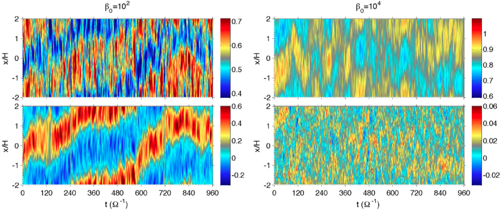
Figure 1.— Time evolution of the radial profiles of mean density $\bar{\rho}$ (top) and mean vertical magnetic field $\bar{B}_{z}$ (bottom) in the midplane region from the ideal MHD, vertically stratified simulations of Bai & Stone (2013a). Left and right panels correspond to runs B2 (midplane $\beta_{0}=10^{2}$) and B4 (midplane $\beta_{0}=10^{4}$) in that paper. The average is taken azimuthally and vertically within $z=\pm 2H$. The color scales are centered at the mean value, and span the same range relative to the mean. This Figure may be viewed in parallel with the top and bottom panels in Figure 7 of Bai & Stone (2013a).

Magnetic flux concentration by MRI turbulence is evident in earlier shearing-box as well as global simulations containing net vertical magnetic flux, although it has not been systematically studied in the literature. For instance, we show in Figure 1 the time evolution of radial profiles for the mean gas density $\bar{\rho}$ and the mean vertical magnetic field $\bar{B}_{z}$ around disk midplane extracted from runs B2 and B4 in Bai & Stone (2013a). These are isothermal ideal magnetohydrodynamic (MHD) stratified shearing-box simulations of the MRI in the presence of relatively strong net vertical magnetic flux. The net vertical field is characterized by $\beta_{0}$, the ratio of gas to magnetic pressure (of the net vertical field) at the disk midplane, with $\beta_{0}=100$ and $10^{4}$ respectively. We see from the top panels that strong zonal flows are produced with density variations of about $30\%$ and $5\%$ around the mean values respectively. The bottom panel shows the corresponding magnetic flux distribution. Concentration of magnetic flux in low-density region of the zonal flow is obvious when $\beta_{0}=10^{2}$, and the high-density region contains essentially zero net vertical magnetic flux. With weaker net vertical field $\beta_{0}=10^{4}$, magnetic flux concentration is still evident but weaker. We emphasize that the systems are highly turbulent where the level of density and magnetic fluctuations is much stronger than their mean values (see Figures 3 and 4 of Bai & Stone, 2013a).

In this work, we systematically explore the phenomenon of magnetic flux concentration by performing a series of local shearing-box simulations (Section 2), both in the ideal MHD regime and in the non-ideal MHD regime with ambipolar diffusion as a proxy for the outer regions of PPDs. All simulations are unstratified and include net vertical magnetic flux. A phenomenological model is presented in Section 3 to address the simulation results. Using this model, we systematically explore parameter space in Section 4. While we focus on unstratified simulations in this work, we have tested that the phenomenological model can be applied equally well to stratified simulations such as shown in Figure 1. A possible physical mechanism for magnetic flux concentration, together with its astrophysical implications are discussed in Section 5. We conclude in Section 6.

2. Magnetic Flux Concentration in Shearing-Box Simulations

We first perform a series of unstratified 3D shearing-box simulations using the Athena MHD code (Stone et al., 2008). The orbital advection scheme (Stone & Gardiner, 2010) is always used to remove location-dependent truncation error and increase the time step (Masset, 2000; Johnson et al., 2008). The MHD equations are written in Cartesian coordinates for a local disk patch in the corotating frame with angular velocity $\Omega$. With $(x,y,z)$ denoting the radial, azimuthal and vertical coordinates, the equations read

$$\frac{\partial\rho}{\partial t}+\nabla\cdot(\rho{\boldsymbol{v}})+v_{K}\frac{\partial\rho}{\partial y}=0\ ,$$ (1)

$$\frac{\partial\rho{\boldsymbol{v}}}{\partial t}+v_{K}\frac{\partial\rho{\boldsymbol{v}}}{\partial y}+\nabla\times(\rho{\boldsymbol{v}}{\boldsymbol{v}}+{\sf T})=-\frac{1}{2}\rho\Omega v_{x}{\boldsymbol{e}}_{y}+2\rho\Omega v_{y}{\boldsymbol{e}}_{x}\ ,$$ (2)

$$\frac{\partial{\boldsymbol{B}}}{\partial t}=-\frac{3}{2}B_{x}\Omega{\boldsymbol{e}}_{y}+\nabla\times\bigg{[}{\boldsymbol{v}}\times{\boldsymbol{B}}+\frac{({\boldsymbol{J}}\times{\boldsymbol{B}})\times{\boldsymbol{B}}}{\gamma\rho_{i}\rho}\bigg{]}\ ,$$ (3)

where ${\sf T}\equiv(P+B^{2}/2){\sf I}-{\boldsymbol{B}}{\boldsymbol{B}}$ is the total stress tensor, $\rho$, $P$, $v_{K}$, ${\boldsymbol{v}}$ and ${\boldsymbol{B}}$ denote gas density, pressure, background Keplerian velocity, background subtracted velocity, and magnetic field, respectively. We adopt an isothermal equation of state $P=\rho c_{s}^{2}$ with $c_{s}$ being the sound speed. The unit for magnetic field is such that magnetic permeability $\mu=1$, and ${\boldsymbol{J}}=\nabla\times{\boldsymbol{B}}$ is the current density. The disk scale height is defined as $H\equiv c_{s}/\Omega$. We set $\rho_{0}=\Omega=c_{s}=H=1$ in code units, where $\rho_{0}$ is the mean gas density. The last term in the induction equation is due to ambipolar diffusion (AD), with $\gamma$ being the coefficient for momentum transfer in ion-neutral collisions, and $\rho_{i}$ is the ion density. The strength of AD is measured by the Elsasser number $Am\equiv\gamma\rho_{i}/\Omega$, the frequency that a neutral molecule collides with the ions normalized to the disk orbital frequency (Chiang & Murray-Clay, 2007). We consider both the ideal MHD regime, which corresponds to $Am\rightarrow\infty$, and the non-ideal MHD regime with $Am\sim 1$, appropriate for the outer regions of PPDs (Bai, 2011a, b).

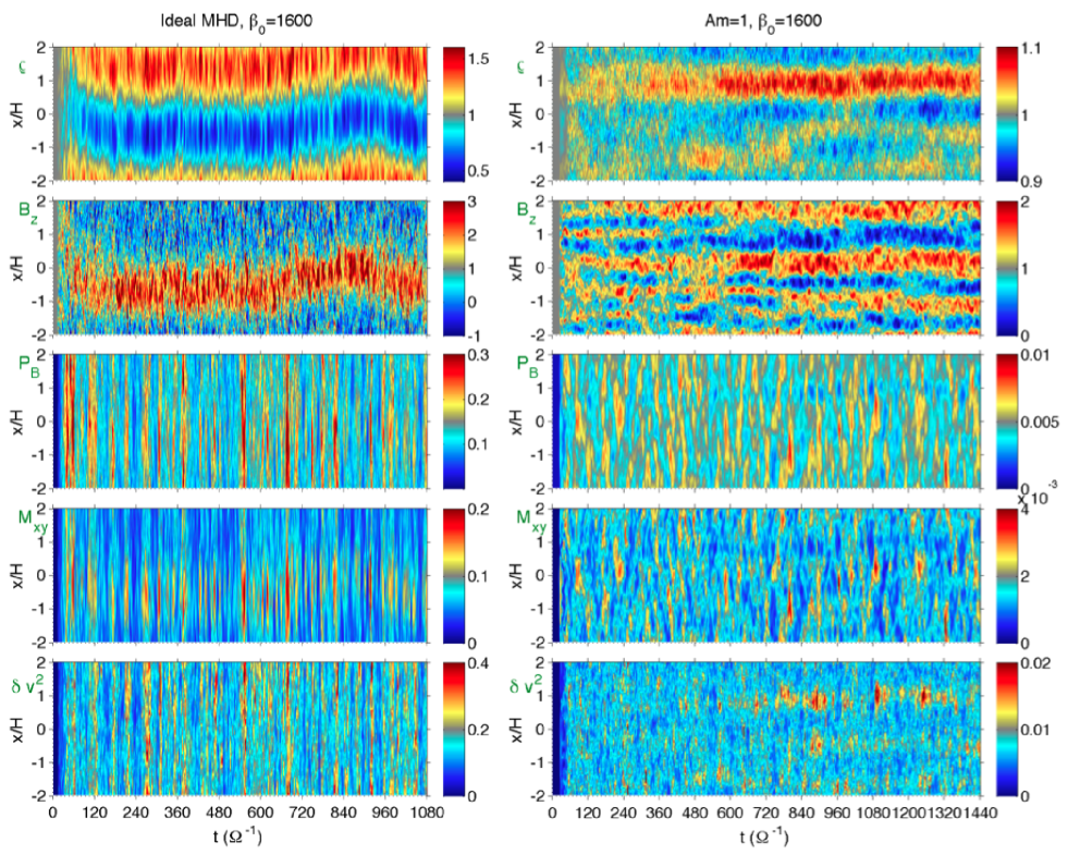
Figure 2.— Time evolution of the radial profiles of main diagnostic quantities from our fiducial ideal MHD run ID-4-16 (left) and fiducial non-ideal MHD run AD-4-16 (right). For each run, from top to bottom, we show the evolution of mean density $\bar{\rho}$, normalized mean vertical magnetic field $\bar{B}_{z}/B_{z0}$, magnetic pressure $P_{B}$, Maxwell stress $M_{xy}$, and turbulent velocity fluctuation $\delta v^{2}=\delta v_{x}^{2}+\delta v_{z}^{2}$.

All our simulations contain net vertical magnetic field $B_{z0}$, measured by initial plasma $\beta_{0}=2P_{0}/B_{z0}^{2}$, the ratio of gas pressure to the magnetic pressure of the net vertical field. We perform a total of 9 runs listed in Table 1. Typical simulation run time ranges from $T=1080\Omega^{-1}$ ($\sim 172$ orbits) to $T=2700\Omega^{-1}$ ($\sim 430$ orbits). Physical run parameters include $\beta_{0}$ and $Am$, while numerical parameters include simulation box size and resolution. Fiducially, we adopt box size of $L_{x}\times L_{y}\times L_{z}=4H\times 4H\times H$, resolved with $192\times 96\times 48$ cells for ideal MHD simulations. For non-ideal MHD simulations, we increase the resolution to $256\times 128\times 64$ cells, which helps better resolve the MRI turbulence (see discussion below). We also explore the effect of horizontal domain size by varying $L_{x}$ from $2H$ to $12H$ while keeping the same resolution (and $L_{y}=\max[L_{x},4H]$). We set $\beta_{0}=1600$ as the standard value, but we also consider $\beta_{0}=400$ and $6400$ for comparison.

All simulations quickly saturate into the MRI turbulence in a few orbits. Standard diagnostics of the MRI include the Maxwell stress

$$M_{xy}\equiv-B_{x}B_{y}\ ,$$ (4)

and the Reynolds stress $\rho v_{x}v_{y}$. Their time and volume averaged values normalized by pressure give the Shakura-Sunyaev parameters $\alpha_{\rm Max}$ and $\alpha_{\rm Rey}$ respectively. In Table 1, we list these values for all our simulations, averaged from $t=360\Omega^{-1}$ onward. Also listed is the plasma $\beta$ parameter, ratio of gas to magnetic pressure at the saturated state. We see that in both ideal and non-ideal MHD runs, $\alpha_{\rm Max}$ and $\alpha_{\rm Rey}$ increases with net vertical magnetic flux, as is well known (Hawley et al., 1995; Bai & Stone, 2011). Also, they all roughly satisfy the empirical relation $\alpha\beta\approx 1/2$ in both ideal MHD and non-ideal MHD cases (Blackman et al., 2008; Bai & Stone, 2011), where $\alpha=\alpha_{\rm Max}+\alpha_{\rm Rey}$.

To ensure that our simulations have sufficient numerical resolution, we have computed the quality factor $Q_{z}\equiv\lambda_{\rm MRI}/\Delta z$ (Noble et al., 2010), where $\lambda_{\rm MRI}$ is the characteristic MRI wavelength based on the total (rms) vertical magnetic field strength. For the most unstable wavelength in ideal MHD, we have $\lambda_{\rm MRI}=9.18\beta_{z}^{-1/2}$ (Hawley et al., 1995), where $\beta_{z}=2P/\overline{B_{z}^{2}}$ is the plasma $\beta$ parameter for the vertical field component. In non-ideal MHD with $Am=1$, we find $\lambda_{\rm MRI}=17.47\beta_{z}^{-1/2}$ (Bai & Stone, 2011). Similarly, one can define $Q_{y}\equiv\lambda_{c}/\Delta y$, where $\lambda_{c}$ is defined the same way as $\lambda_{\rm MRI}$ but using $\beta_{\phi}$ instead of $\beta_{z}$. In general, the MRI is well resolved when $Q_{y}\gtrsim 20$ and $Q_{z}\gtrsim 10$ (Hawley et al., 2011). We find that in all our simulations are well resolved based on this criterion. Further details are provided in Section 4.

In Figure 2, we show the time evolution of the radial profiles of various diagnostic quantities for our fiducial ideal and non-ideal MHD runs. The results are discussed below. Other runs will be discussed in Section 4.

2.1. The Ideal MHD Case

In this ideal MHD run, we see that a very strong zonal flow is produced, with density contrast up to $50\%$. In the mean time, there is a strong anti-correlation between gas density and mean vertical magnetic field, with most magnetic flux concentrated in the low density regions. In this fiducial run with radial box size $L_{x}=4H$, there is just one single “wavelength” of density and mean field variations. The phase of the pressure maxima drifts slowly in a random way over long timescales, accompanied by a slow radial drift of the mean field profile; but overall, the system achieves a quasi-steady-state in terms of density and magnetic flux distributions.

Combined with Figure 1, we see that both unstratified and stratified shearing-box simulations show similar phenomenon of magnetic flux concentration and zonal flows. This fact indicates that the same physics is operating, independent of buoyancy. We stress that the mean vertical field, even in the highly concentrated region, is much weaker than the rms vertical field from the MRI turbulence. Therefore, the physics of magnetic flux concentration lies in the intrinsic properties of the MRI turbulence.

From the last three panels on the left of Figure 2, we see that the action of the Maxwell stress (which is the driving force of the zonal flow) is bursty. Such behavior corresponds to the recurrence of the channel flows followed by dissipation due to magnetic reconnection (Sano & Inutsuka, 2001). The Maxwell stress is most strongly exerted in regions where magnetic flux is concentrated. Interestingly, magnetic pressure shows bursty behavior similar to the Maxwell stress, but its strength does not show obvious signs of radial variation. On the other hand, turbulent velocity in the $x-z$ plane, given by $\delta v^{2}=\delta v_{x}^{2}+\delta v_{z}^{2}$, is strongest in regions with weaker magnetic flux during each burst. While we are mostly dealing with time-averaged quantities in this work, one should keep in mind about such variabilities on timescales of a few orbits.

Table 1List of all shearing-box simulations

Run	Box size ($H$)	$\beta_{0}$	$Am$	$\alpha_{\rm Max}$	$\alpha_{\rm Rey}$	$\langle\beta\rangle$	$\Delta\rho/\rho_{0}$	$\overline{B}_{z}^{\rm Max}/B_{z0}$	$\alpha_{m}$	$\alpha_{t}$	$Q^{\prime}$	$\alpha_{xy}$	$t\ (\Omega^{-1})$
ID-4-4	$4\times 4\times 1$	$400$	$\infty$	$0.15$	$0.055$	$3.6$	$0.26$	$1.8$	$0.22$	$0.054$	$-0.11$	$-0.12$	$360-660$
ID-4-16	$4\times 4\times 1$	$1600$	$\infty$	$0.070$	$0.026$	$7.4$	$0.37$	$2.2$	$0.086$	$0.033$	$-0.081$	$-0.072$	$360-720$
ID-4-64	$4\times 4\times 1$	$6400$	$\infty$	$0.034$	$0.010$	$14$	$0.23$	$2.1$	$0.032$	$0.010$	$-0.050$	$-0.033$	$600-780$
ID-2-16	$2\times 4\times 1$	$1600$	$\infty$	$0.083$	$0.022$	$5.7$	$0.014$	$1.33$	$--$	$--$	$---$	$--$	$480-600$
ID-8-16	$8\times 8\times 1$	$1600$	$\infty$	$0.069$	$0.025$	$7.1$	$0.44$	$2.0$	$0.014$	$0.032$	$-0.089$	$-0.069$	$1260-1500$
ID-16-16	$16\times 16\times 1$	$1600$	$\infty$	$0.070$	$0.024$	$6.9$	$0.29$	$1.4$	$--$	$--$	$--$	$--$	$1170-1350$
AD-4-16	$4\times 4\times 1$	$1600$	$1$	$1.5$E$-3$	$9.1$E$-4$	$2.1$E+$2$	$0.061$	$1.6$	$5.6$E$-3$	$1.1$E$-3$	$-0.093$	$2.6$E$-3$	$1080-1440$
AD-4-64	$4\times 4\times 1$	$6400$	$1$	$4.8$E$-4$	$6.0$E$-4$	$5.0$E+$2$	$0.081$	$2.6$	$1.6$E$-3$	$4.9$E$-4$	$-0.064$	$1.2$E$-3$	$1200-1440$
AD-2-64	$2\times 4\times 1$	$6400$	$1$	$4.4$E$-4$	$4.1$E$-4$	$5.3$E$+2$	$0.024$	$2.0$	$7.6$E$-3$	$5.8$E$-4$	$-0.048$	$1.1$E$-3$	$210-450$

2.2. The Non-ideal MHD Case

On the right of Figure 2, we show the time evolution of the radial profiles of main diagnostic quantities from our fiducial non-ideal MHD simulation AD-4-16. Zonal flows and magnetic flux concentration are obvious from the plots. One important difference from the ideal MHD case is that the scale that magnetic flux concentrates is much smaller: we observe multiple shells of concentrated magnetic flux whose width is around $0.5H$ or less. The shells may persist, split, or merge during the evolution, while their locations are well correlated with the troughs in the radial density profile. Many other aspects of the evolution are similar to the ideal MHD case, such as the action of Maxwell stress, and the distribution of $P_{B}$ and $\delta v^{2}$. These flux-concentrated shells closely resemble the shells of magnetic flux observed in stratified simulations shown in Figure 8 of Bai (2014). Again, the similarities indicate that the physics of magnetic flux concentration is well captured in unstratified simulations.

In our unstratified simulations, the zonal flow is weaker than in the ideal MHD cases, where the amplitude of density variations is typically $10\%$ or less. The level of radial density variations in stratified simulations is typically larger (Simon & Armitage, 2014; Bai, 2014). Meanwhile, it appears that magnetic flux concentration is more complete in stratified simulations: most of the magnetic flux is concentrated into the shells, while other regions have nearly zero net vertical flux (again see Figure 8 of Bai, 2014). Also, the flux-concentrated shells are more widely separated in stratified simulations. Note that these stratified simulations contain an ideal-MHD, more strongly magnetized and fully MRI turbulent surface layer, which may affect the strength of the zonal flow at disk midplane (via the Taylor-Proudman theorem) as well as the level of magnetic flux concentration. Nonetheless, addressing these differences is beyond the scope of this work.

Finally, we note that the zonal flow and magnetic flux concentration phenomena were already present in our earlier AD simulations (Bai & Stone, 2011; Zhu et al., 2014). These simulations either focused on the Shakura-Sunyaev $\alpha$ parameter, or the properties of the MRI turbulence, while the radial distribution of magnetic flux was not addressed.

3. A Phenomenological Model

In this section, we consider our fiducial run ID-4-16 for a detailed case study. We take advantage of the fact that the system achieves a quasi-steady-state in its radial profiles of density and magnetic flux, and construct a phenomenological, mean-field interpretation on magnetic flux concentration and enhanced zonal flows. We use overbar to denote quantities averaged over the $y-z$ dimensions (and certain period of time), which have radial dependence. We use $\langle\cdot\rangle$ to represent time and volume averaged values in the entire simulation domain at the saturated state of the MRI turbulence. In Figure 3 we show the radial profiles of some main diagnostic quantities. They are obtained by averaging from $t=360\Omega^{-1}$ to $720\Omega^{-1}$, where the density and magnetic flux profiles approximately maintain constant phase. Detailed analysis are described below.

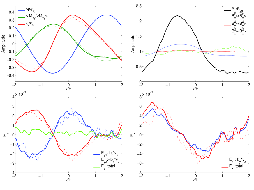
Figure 3.— Radial profiles of various quantities in the saturated state of run ID-4-16, as indicated in the legends in each panel. Dashed-dotted lines are fits to the measured profiles based on the phenomenological model in Section 3.

3.1. Force balance

Zonal flow is a result of geostrophic balance between radial pressure gradient and the Coriolis force

$$\frac{c_{s}^{2}}{2\Omega}\frac{\partial\overline{\rho}}{\partial x}=\overline{\rho}\overline{v}_{y}\approx\rho_{0}\overline{v}_{y}\ .$$ (5)

From the top left panel of Figure 3, we see that the above formula accurately fits the measured profile of $\overline{v}_{y}$.

The pressure gradients are driven by radial variations of the Maxwell stress, balanced by mass diffusion (Johansen et al., 2009). Using $D_{m}$ to denote the mass diffusion coefficient, one obtains

$$\frac{2}{\Omega}\frac{\partial\overline{M}_{xy}}{\partial x}=-D_{m}\frac{\partial\overline{\rho}}{\partial x}\ .$$ (6)

Therefore, in a periodic box, the density variation should be anti-correlated with the Maxwell stress. Asserting $D_{m}\equiv\alpha_{m}c_{s}H$ and assuming $\alpha_{m}$ is a constant, we obtain

$$\frac{\Delta\overline{M}_{xy}}{\langle M_{xy}\rangle}\approx-\frac{\alpha_{m}}{2\alpha_{\rm Max}}\frac{\Delta\overline{\rho}}{\rho_{0}}\ ,$$ (7)

where $\Delta\overline{A}\equiv\overline{A}-\langle A\rangle$ for any quantity $A$.

We can fit the mass diffusion coefficient based on Equation (7), and obtain $\alpha_{m}\approx 1.2\alpha_{\rm Max}\approx 0.086$. Also from the top left panel of Figure 3, we see that the fitting result agrees extremely well with the measured profile of $\overline{M}_{xy}$.

3.2. Magnetic Flux Evolution

The evolution of vertical magnetic flux is controlled by the toroidal electric field via the induction equation (3)

$$\frac{\partial\overline{B}_{z}(x)}{\partial t}=-\frac{\partial\overline{E}_{y}}{\partial x}\ ,$$ (8)

where in ideal MHD, the toroidal electric field can be decomposed into

$$\overline{E}_{y}=\overline{E}_{y1}+\overline{E}_{y2}=\overline{v_{x}B_{z}}-\overline{v_{z}B_{x}}\ .$$ (9)

In the above, the first term describes the advective transport of magnetic flux by turbulent resistivity

$$\overline{E}_{y1}=\overline{v_{x}B_{z}}\approx\eta_{t}\overline{J}_{y}=-\eta_{t}\partial_{x}\overline{B}_{z}\ ,$$ (10)

where $\eta_{t}\equiv\alpha_{t}c_{s}H$ is the turbulent resistivity. The outcome is that accumulation of magnetic flux tends to be smeared out. We can fit the value of $\alpha_{t}$ from the profiles of $\overline{B}_{z}$ and $\overline{E}_{y1}$ to obtain $\alpha_{t}\approx 0.033$, which is the same order as $\alpha_{\rm Max}$. While the data are somewhat noisy, we see from the bottom left panel of Figure 3 that the profile of $\overline{E}_{y1}$ is well fitted from Equation (10). This is the basic principle for measuring turbulent resistivity from the MRI (Guan & Gammie, 2009; Lesur & Longaretti, 2009; Fromang & Stone, 2009).

The second term in (9) describes the generation of vertical field by tilting the radial field. Since we expect ${\overline{v}}_{z}=0$ and ${\overline{B}}_{x}=0$ in the MRI turbulence, its contribution must come from a correlation between $v_{z}$ and $B_{x}$, which is primarily responsible for magnetic flux accumulation. The fact that the system achieves a quasi-equilibrium state indicates that their sum $\overline{E}_{y}\approx 0$. Therefore, contribution from $\overline{E}_{y2}$ must balance the turbulent diffusion term $\overline{E}_{y1}$. This is indeed the case, as we see from Figure 3.

3.3. Turbulent Diffusivity

The saturated state of the system has a mean toroidal current $\overline{J}_{y}=-\partial\overline{B}_{z}/\partial x$ but zero mean toroidal electric field $\overline{E}_{y}\approx 0$. Applying an isotropic Ohm’s law to the system would yield infinite conductivity. This is obviously not the case. The issue can be resolved if the turbulent conductivity/diffusivity is anisotropic with strong off-diagonal components.

More generally, we write

$$\overline{E}_{i}=\eta_{ik}\overline{J}_{k}\ ,$$ (11)

where $i,j,k$ denote any of the $x,y,z$ components, and one sums over index $k$. Given the mean $\overline{J}_{y}$, we have analyzed all other components of the mean electric field. We find that the mean vertical electric field $\overline{E}_{z}$ is consistent with zero, while there is a non-zero mean radial electric field

$$\overline{E}_{x}=\overline{E}_{x1}+\overline{E}_{x2}=\overline{v_{z}B_{y}}-\overline{\delta v_{y}\delta B_{z}}\ .$$ (12)

Note that in the second term $\overline{E}_{x2}$, we have removed the component $\overline{v}_{y}\overline{B}_{z}$, which corresponds to the advection of vertical field due to disk rotation and is physically irrelevant to the MRI turbulence.

In the bottom right panel of Figure 3, we show the radial profiles of $\overline{E}_{x}$ and $\overline{E}_{x1}$. We see that $\overline{E}_{x}$ is approximately in phase with $-\overline{E}_{y1}$ and $\overline{E}_{y2}$. This observation indicates that at the saturated state, the system is characterized by an anisotropic turbulent diffusivity that is off-diagonal, given by

$$\overline{E}_{x}\approx\eta_{xy}\overline{J}_{y}\ .$$ (13)

We can fit the value of $\eta_{xy}\equiv\alpha_{xy}c_{s}H$ to obtain $\alpha_{xy}\approx-0.072\approx-\alpha_{\rm Max}$. In the bottom right panel of Figure 3, we see that although the fitting result is not perfect, it captures the basic trend on the radial variations of $\overline{E}_{x}$. It is satisfactory since some features can be smoothed out over the time average due to the (small) phase shift of the density/magnetic flux profiles.

Anisotropic diffusivities in MRI turbulence have been noted in Lesur & Longaretti (2009), who measured most components of the diffusivity tensor by imposing some fixed amplitude mean field variations in Fourier space. In particular, they found that the value of $\eta_{xy}$ is typically negative, and the value of $|\alpha_{xy}|$ can be a substantial fraction of $\alpha_{\rm Max}$. Also, they found that $|\eta_{xy}|$ is typically a factor of several larger than the diagonal component, which is our equivalence of $\eta_{t}$. Our measurements of $\eta_{xy}$ are consistent with their results.

3.4. Connection between Anisotropic Diffusivity and Magnetic Flux Concentration

We see from the bottom right panel of Figure 3 that contributions to $\overline{E}_{x}$ is completely dominated by $\overline{E}_{x1}=\overline{v_{z}B_{y}}$, indicating a correlation between $v_{z}$ and $B_{y}$. In Section 3.2, we see that magnetic flux concentration is mainly maintained by $\overline{E}_{y2}=-\overline{v_{z}B_{x}}$, indicating an anti-correlation between $v_{z}$ and $B_{x}$. Since $B_{y}$ and $-B_{x}$ are correlated in the MRI turbulence (to give the Maxwell stress $-\overline{B_{x}B_{y}}>0$), it is not too surprising that the two correlations are related to one another: $\overline{E}_{y2}$ and $\overline{E}_{x1}$ are in phase as we see in Figure 3.

Our analysis suggests that magnetic flux concentration is a direct consequence of the anisotropic diffusivity/conductivity in the MRI turbulence. In addition to turbulent resistivity given by $\overline{E}_{y1}$, another anisotropic component, resulting from correlations between $v_{z}$ and the horizontal magnetic field, contributes to both $\overline{E}_{y2}$ and $\overline{E}_{x1}$. The latter exhibits as $\eta_{xy}$, while the former acts to concentrate vertical magnetic flux.

3.5. Analogies to the Hall Effect

We note that the generation of $\overline{E}_{x}$ from $\overline{J}_{y}$ in the presence of mean vertical field is analogous to the classical Hall effect. If we empirically set $\eta_{xy}\equiv QB_{z0}$, the electric field in the saturated state may be written as

$$\overline{\boldsymbol{E}}\approx Q\overline{\boldsymbol{J}}\times\overline{\boldsymbol{B}}\ .$$ (14)

Since only $\overline{J}_{y}$ and $\overline{B}_{z}$ are non-zero, this leads to a net $\overline{E}_{x}$, consistent with our measurement.

The analogy above prompts us to draw another analogy between the microscopic Hall effect and magnetic flux concentration, which was demonstrated in Kunz & Lesur (2013). For the microscopic Hall effect, the Hall electric field can be written as

$$\overline{\boldsymbol{E}}^{h}\approx Q^{\prime}\overline{{\boldsymbol{J}}\times{\boldsymbol{B}}}\ .$$ (15)

It generates a mean toroidal electric field via

$$\overline{E}_{y}^{h}\approx Q^{\prime}\overline{B_{x}(\partial_{x}{B_{y}})}\approx-Q^{\prime}\frac{\partial\overline{M}_{xy}}{\partial x}\ .$$ (16)

We can fit $\overline{E}_{y2}$ using the above relation to obtain $Q^{\prime}\approx-0.080$ in code unit. As seen in Figure 3, the radial profile of $\overline{E}_{y2}$ is fitted very well. Also note that both $Q$ and $Q^{\prime}$ are negative based on our fitting results to $\overline{E}_{x}$ and $\overline{E}_{y2}$. While different phenomenological considerations are used to arrive at Equations (14) and (15), the directionality of the two electric field components is in line with the Hall-like interpretation.

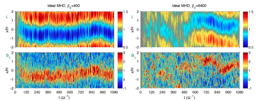
Figure 4.— Time evolution of the radial profiles of $\overline{\rho}$ (top) and $\overline{B}_{z}/B_{z0}$ (bottom) from our ideal MHD runs with different $\beta_{0}$: ID-4-4 (left) and ID-4-64 (right).

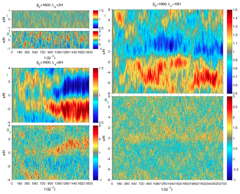
Figure 5.— Time evolution of the radial profiles of $\overline{\rho}$ and $\overline{B}_{z}/B_{z0}$ from our ideal MHD runs with different $L_{x}$: ID-2-16 (top left), ID-8-16 (bottom left), ID-16-16 (right).

Encouraged by the analogies above, if we insert Equation (16) as an ansatz for $\overline{E}_{y2}$, then the evolution of vertical magnetic flux can be written as

$$\frac{\partial\overline{B}_{z}}{\partial t}\approx\bigg{(}\eta_{t}+Q^{\prime}\frac{d\overline{M}_{xy}}{d\overline{B}_{z}}\bigg{)}\frac{\partial^{2}\overline{B}_{z}}{\partial x^{2}}\ .$$ (17)

In general, we expect $\overline{M}_{xy}$ to increase with net vertical flux until the net vertical field becomes too strong: $d\overline{M}_{xy}/d\overline{B}_{z}>0$ ($B_{z}>0$). From our measurement, we have $Q^{\prime}<0$. Therefore, the second term in Equation (17) acts as anti-diffusion of vertical magnetic flux. It is likely that this term dominates over turbulent diffusion at the initial evolutionary stage to trigger magnetic flux concentration, while turbulent diffusion catches up at later stages when sufficient magnetic flux concentration is achieved. Together with Equation (7), we see that the gradient of Maxwell stress is responsible for both launching of the zonal flow and magnetic flux concentration. This provides a phenomenological interpretation why magnetic flux always concentrates toward low-density regions. Given our crude phenomenological treatment, however, we can not provide more detailed descriptions on the flux concentration process and phase evolution, nor can we explain its saturation scale and amplitude without involving many unjustified speculations.

Our Equation (17) closely resembles Equation (26) of Kunz & Lesur (2013), which were used to explain magnetic flux concentration due to the microscopic Hall effect. The counterpart of our $Q^{\prime}$ in their paper is positive. Therefore, strong concentration of magnetic flux occurs only when the Hall effect and net vertical field become sufficiently strong (so that $M_{xy}$ decreases with $B_{z}$). In our case, since $Q^{\prime}$ is negative, magnetic flux concentration is expected even for relatively weak net vertical field.

3.6. Summary

In sum, we have decomposed the turbulent diffusivity from the MRI turbulence into two ingredients. There is a conventional, Ohmic-like turbulent resistivity $\eta_{t}$. In addition, we find correlations of $v_{z}$ with $B_{y}$ and $B_{x}$ in the presence of vertical magnetic flux gradient. The former leads to an anisotropic diffusivity, which is analogous to the the classical Hall effect. The latter effectively leads to anti-diffusion of vertical magnetic flux, which is responsible for magnetic flux concentration, and is analogous to the the microscopic Hall effect.

We emphasize that anisotropic turbulent conductivity/diffusivity is an intrinsic property of the MRI turbulence. While we draw analogies with the Hall effect, it represents an phenomenological approach and simply reflects our ignorance about the MRI turbulence. The readers should not confuse this analogy with the physical (classical or microscopic) Hall effect, which would lead to polarity dependence (on the sign of $B_{z0}$). Magnetic flux concentration, on the other hand, has NO polarity dependence.

4. Parameter Exploration

The main results of a series of simulations we have performed to explore parameter space are summarized in Table 1. We follow the procedure in Section 3 to analyze the properties related to zonal flows and magnetic flux concentration. In doing so, we choose a specific time period in each run where the density and magnetic flux profiles maintain approximately constant phase. They are listed in the last column of the Table. In many cases, multiple periods can be chosen, and we confirm that the fitting results are insensitive to period selection. To characterize the strength of the zonal flow and magnetic flux concentration, we further include in the table $\Delta\overline{\rho}/\rho_{0}$, the relative amplitude of radial density variations, and $\overline{B}_{z}^{\rm Max}/B_{z0}$, the ratio of maximum vertical field in the time-averaged radial profile to its initial background value. Runs ID-2-16 and ID-16-16 never achieve a quasi-steady state in their density and magnetic flux distribution, we thus simply measure $\Delta\overline{\rho}/\rho_{0}$ and $\overline{B}_{z}^{\rm Max}/B_{z0}$ over some brief periods, leaving other fitting parameters blank in the Table.

4.1. Ideal MHD Simulations

All our ideal-MHD simulations have achieved numerical convergence based on the quality factor criterion discussed in Section 2. In particular, in the run with weakest net vertical field ID-4-64, we find $\overline{Q}_{y}>45$ and $\overline{Q}_{z}>25$ for any $x$, meaning that the resolution is about twice more than needed to properly resolve the MRI. Runs with stronger net vertical field give further larger quality factors. Below we discuss the main simulation results.

4.1.1 Dependence on Net Vertical Field Strength

We first fix the simulation domain size ($L_{x}=4H$) and vary the strength of the net vertical magnetic field to $\beta_{0}=400$ and $\beta_{0}=6400$. The time evolution of $\overline{\rho}$ and $\overline{B}_{z}/B_{z0}$ in the two runs are shown in Figure 4. We see that in general, enhanced zonal flow requires relatively strong net vertical magnetic field. Our run ID-4-64 with $\beta_{0}=6400$ has notably weaker density contrast of $\sim 20\%$ compared with $\sim 40\%$ in our fiducial run ID-4-16. It also takes longer time for strong concentration of magnetic flux to develop. This is in line with the vertically stratified simulations shown in Figure 1. In the limit of zero net vertical flux, the density contrast is further reduced to $\sim 10\%$ (Johansen et al., 2009; Simon et al., 2012).

For the selected time periods, we find that the phenomenological description in Section 3 works well of all ideal MHD simulations. There is a systematic trend that the mass diffusion coefficient $\alpha_{m}$, turbulent resistivity $\alpha_{t}$, $Q^{\prime}$ and $|\alpha_{xy}|$ all increase with increasing net vertical field. In particular, $\alpha_{t}$ and $\alpha_{xy}$ roughly scale in proportion with $\alpha_{\rm Max}$.

We do not extend our simulations to further weaker net vertical field, where the MRI would be under-resolved. On the other hand, we note that without net vertical magnetic flux, oppositely directed mean vertical magnetic fields tend to decay/reconnect, rather than grow spontaneously (Guan & Gammie, 2009). Therefore, concentration of vertical magnetic flux occurs only when there is a net vertical magnetic field threading the disk.

Combining both our unstratified simulation results and the results from stratified simulations of shown in Figure 1, we expect strong concentration of magnetic flux and enhanced zonal flow to take place for net vertical field $\beta_{0}\lesssim 10^{4}$.

4.1.2 Dependence on Radial Domain Size

In our fiducial run ID-4-16, only one single “wavelength” of density and magnetic flux variations fit into our simulation box. We thus proceed to perform additional simulations varying the radial domain size, and show the time evolution of their density and magnetic flux profiles in Figure 5.

We first notice that when using a smaller box with $L_{x}=2H$, the zonal structures become much weaker. They appear to be more intermittent, have finite lifetime, and undergo rapid and random radial drift. One can still see that magnetic flux is concentrated toward low density regions, although the trend is less pronounced than that in our fiducial run. Also, the system never achieves a quasi-steady state on its magnetic flux distribution. We note that most previous unstratified simulations of the MRI adopt even smaller radial domain size with $L_{x}=H$ (e.g., Hawley et al., 1995; Fleming et al., 2000; Sano & Inutsuka, 2001; Lesur & Longaretti, 2007; Simon et al., 2009). Therefore, the intermittent features discussed above would make signatures of magnetic flux concentration hardly noticeable in these simulations. We also note that the phenomenon of magnetic flux concentration should occur in earlier unstratified simulations with relatively large radial domain such as in Bodo et al. (2008) and Longaretti & Lesur (2010). Nonetheless, these works have mostly focused on the volume averaged turbulent transport coefficients rather than sub-structures in the radial dimension.

Enlarging the radial domain size to $L_{x}=8H$, we see that the system initially develops two “wavelengths” of zonal structures ($t=300-1000\Omega^{-1}$), with magnetic flux concentrated into two radial locations corresponding to the density minima. Later on, however, the two modes merge into one single mode with much stronger density variation. The magnetic flux in the two radial locations also merge to reside in the new density trough. From this time, the system achieves a quasi-steady state configuration. We find that for turbulent diffusivities, our model provides excellent fits, and the values of $\alpha_{t}$, $Q^{\prime}$ and $\alpha_{xy}$ agree with those in the fiducial run ID-4-16 very well. This indicates well converged basic turbulent properties with simulation domain size, and our phenomenological description on magnetic flux concentration works reasonably well in a wider simulation box. On the other hand, we find that Equation (7) no longer yields a good fit between the density and Maxwell stress profiles, leaving the value of $\alpha_{m}$ poorly measured (the reported value represents an underestimate). This is most likely due to the more stochastic nature of the forcing term (Maxwell stress) in a wider simulation box, which has been discussed in Johansen et al. (2009).

Further increasing the radial domain size to $L_{x}=16H$, we find that the system initially breaks into multiple zonal structures. Magnetic flux still concentrates toward low-density regions, but the density and magnetic flux profiles show long-term evolutions. Even by running the simulation for more than 400 orbits, no quasi-steady configuration is found. The later evolution of the system is still dominated a single “mode” of zonal structure in the entire radial domain, but there are more substructures associated with multiple peaks of magnetic flux distribution. The overall level of magnetic flux concentration is weaker, with typical $\overline{B}_{z}^{\rm Max}/B_{z0}\sim 1.5$ or less, and the typical scale of individual magnetic flux substructure is around $\sim 2H$. While we may speculate that this simulation better represents realistic (fully-ionized) disks, we also note that the simulation box size of this run is already large enough that the local shearing-sheet formulation would fail if the disk is not too thin (e.g., aspect ratio $H/R\lesssim 0.03$), and we have not included vertical stratification. Overall, in the ideal MHD case, the properties of the zonal flow and magnetic flux concentration do not converge with the box size in shearing-box simulations.

Finally, we notice that evidence of magnetic flux concentration is already present in earlier global unstratified simulations with net vertical flux. Hawley (2001) found in his simulations the formation of a dense ring near the inner radial boundary and various low density gaps (i.e., zonal flows) within the disk, which were tentatively attributed to a type of “viscous” instability. Steinacker & Papaloizou (2002) obtained similar results and identified the trapping of vertical magnetic flux in the density gaps, although they did not pursue further investigation. While shearing-box simulation results do not converge with box size, these global unstratified simulation results lend further support to the robustness of magnetic flux concentration in more realistic settings.

4.2. Non-ideal MHD Simulations

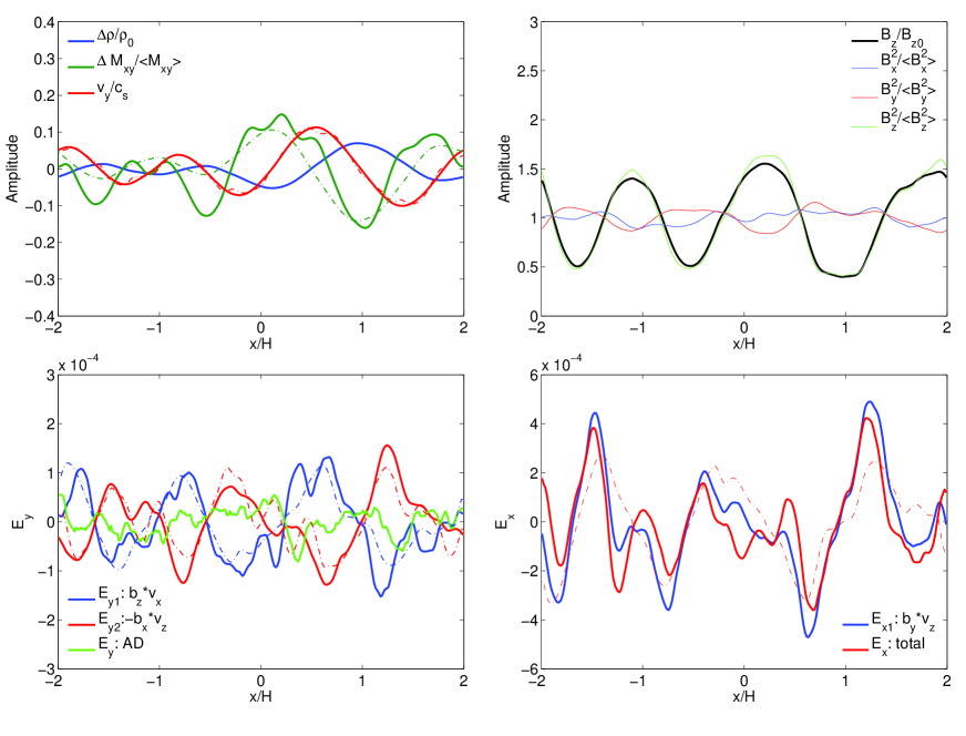
Figure 6.— Radial profiles of various quantities in the saturated state of run AD-4-16, as indicated in the legends in each panel. Dashed-dotted lines are fits to the measured profiles based on the phenomenological model in Section 3. Note that the green curve in the bottom left panel now shows $E_{y}$ due to AD.

With strong AD, we first show in Figure 6 the radial profiles of main diagnostics from our fiducial run AD-4-16, with fitting results over plotted, which compliments our discussions in Section 2.2. We first notice from the top right panel that because the MRI turbulence is weaker due to AD, the mean vertical field dominates over the rms fluctuations of the vertical field in the flux-concentrated shells. This is also the case in most stratified shearing-box simulations for the outer regions of PPDs in Bai (2014). Magnetic fluctuations in $B_{x}$ and $B_{y}$ do not show strong trend of radial variations.

Secondly, we find that for this run, magnetic flux concentration is still mainly due to turbulent motions. In the bottom left panel of Figure 6, we also show $\overline{E}_{y}^{\rm AD}$, the toroidal electric field resulting from AD. We see that the contribution from $\overline{E}_{y}^{\rm AD}$ is small compared with the other two components $\overline{E}_{y1}$ and $\overline{E}_{y2}$. Therefore, the phenomenological description in Section 3 is equally applicable in the non-ideal MHD case. It provides reasonable fits in the mean $\overline{E}_{x}$ and $\overline{E}_{y}$ profiles. We will discuss further on the role of AD in Section 4.2.1.

We also notice that while the radial density variation and Maxwell stress are still anti-correlated, they are not well fitted from relation (7). Correspondingly, the mass diffusion coefficient $\alpha_{m}$ is not very well measured. Again, this is likely due to the stochastic nature of the forcing term (Maxwell stress). As we see from Figure 2 (3rd panel on the right), many bursts of the Maxwell stress are exerted over an extended range of the radial domain, covering multiple peaks and troughs in the magnetic flux profile. Although on average, regions with strong magnetic flux concentration have stronger Maxwell stress, the “kicks” they receive are not as coherent as its ideal MHD counterpart (3rd panel on the left). In this situation, it is more appropriate to apply the stochastic description of the zonal flow in Johansen et al. (2009) rather than the simple form of Equation (6).

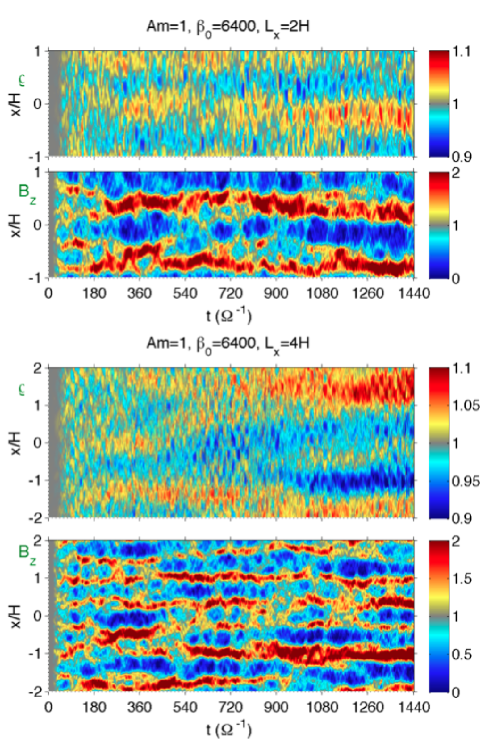
Figure 7.— Time evolution of the radial profiles of $\overline{\rho}$ and $\overline{B}_{z}/B_{z0}$ from our two non-ideal MHD runs with different radial domain size: AD-2-64 (top) and AD-4-64 (bottom).

In Figure 7, we further show the time evolution of density and magnetic flux profiles from two other runs AD-2-64 and AD-4-64 with $\beta_{0}=6400$ and $Am=1$. We see that the evolutionary patterns from the two runs are very similar to each other. They are also qualitatively similar to our run AD-4-16 discussed earlier, with magnetic flux concentrated into thin shells whose sizes are $\lesssim 0.5H$. We have also tested the results with larger box size $L_{x}=6H$, and find very similar behaviors as smaller box runs. This is very different from the ideal MHD case, and provides evidence that the properties of magnetic flux concentration converge with simulation box size down to $L_{x}=2H$ in unstratified simulations. The convergence is mainly due to the small width of the flux-concentrated shells and their small separation. Nevertheless, we again remind the readers that properties of magnetic flux concentration and zonal flows can be different in the more realistic stratified simulations, as mentioned in Section 2.2.

In the bottom panels of Figure 7, we see that the properties of the zonal flow in our run AD-4-64 show long-term evolutions over the more than 100 orbits, and stronger density contrast is developed toward the end of the run (which again may relate to stochastic forcing). Similar long-term evolution behavior was also reported in unstratified simulations of Bai (2014). Despite the value of $\alpha_{m}$ being poorly determined, other quantities $\alpha_{t}$, $\alpha_{xy}$ and $Q^{\prime}$ are found to be similar between the two runs AD-2-64 and AD-4-64. Their values are a factor of $\sim 2$ smaller than in run AD-4-16 with twice the net vertical field, consistent with expectations of weaker turbulence. In addition, we see that magnetic flux concentration is even more pronounced with weaker net vertical field $\beta_{0}=6400$ than with $\beta_{0}=1600$. Combining the results from stratified simulations of Bai (2014), we see that strong magnetic flux concentration can be achieved with very weak net vertical field, at least down to $\beta_{0}=10^{5}$.

We have also computed the quality factors for these two runs with $\beta_{0}=6400$, and find $\overline{Q}_{y}\gtrsim 20$ over the entire simulation domain, $\overline{Q}_{z}\sim 10-15$ in high density regions, and $\overline{Q}_{z}\sim 20-30$ in low density regions. The small $\overline{Q}_{z}$ value in high density regions is mainly due to weaker (rms) vertical field, hence larger $\beta_{z}$, as a result of magnetic flux concentration and zonal flows. We see that the relatively high resolution ($64$ cells per $H$ in $z$) that we have adopted for these non-ideal MHD simulations is necessary to guarantee proper resolution of the MRI over the entire simulation domain, especially the high-density regions of the zonal flow.

Finally, by comparing run AD-4-16 with run ID-4-16, we see that the Maxwell stress $\alpha_{\rm Max}$ is reduced by a factor of $\sim 50$ due to AD. On the other hand, we find that the amplitudes of $\overline{E}_{y1}$ and $\overline{E}_{y2}$ are reduced by just a factor of $\sim 20$. Since both $\alpha_{\rm Max}$ and $\overline{E}_{y}$ result from quadratic combinations of turbulent fluctuations, this fact indicates that while turbulence gets weaker, the correlation between $v_{z}$ and $B_{x}$ becomes tighter in the AD case. To quantify this, we further define

$$\delta_{x}\equiv\frac{\langle|\overline{v_{z}B_{x}}|\rangle}{\langle v_{z}^{2}\rangle^{1/2}\langle B_{x}^{2}\rangle^{1/2}}\ ,\quad\delta_{y}\equiv\frac{\langle|\overline{v_{z}B_{y}}|\rangle}{\langle v_{z}^{2}\rangle^{1/2}\langle B_{y}^{2}\rangle^{1/2}}\ ,$$ (18)

where the overbar indicates averaging over the horizontal and vertical domain at individual snapshots, and the angle bracket indicates further averaging over the radial domain and selected time period in Table 1. For all ideal MHD runs, we consistently find that $\delta_{x}\sim 0.07-0.09$, and $\delta_{y}\sim 0.09-0.11$. For all non-ideal MHD runs, we find $\delta_{x}\sim 0.10-0.11$, and $\delta_{y}\sim 0.14-0.16$. It is clear that non-ideal MHD simulations give larger $\delta$ values. In the ideal MHD case, the actual correlations between $v_{z}$ and $B_{x}$, $B_{y}$ are weaker than indicated by the $\delta$ values due to stronger time fluctuations. Recently, Zhu et al. (2014) noticed that the MRI turbulence with AD has very long correlation time in vertical velocity (see their Figures 9 and 13). The more coherent vertical motion in the AD dominated MRI turbulence might also be related to the stronger correlation between $v_{z}$ and $B_{x}$, $B_{y}$ and efficient magnetic flux concentration.

4.2.1 Role of Ambipolar Diffusion on Magnetic Flux Concentration

As previously discussed, AD appears to play a minor role in magnetic flux concentration in run AD-4-16, as shown in the bottom left panel of Figure 6. On the other hand, we find that with weaker net vertical field as in run AD-4-64 ($\beta_{0}=6400$), AD acts to enhance the level of magnetic flux concentration. In Table 1, we see that the value $\overline{B}_{z}^{\rm Max}/B_{z0}$ is systematically higher in run AD-4-64 compared with run AD-4-16. In Figure 8, we show the radial profiles of $\overline{B}_{z}$ as well as various components of $\overline{E}_{y}$. We see that vertical flux is squeezed into thiner shells with much sharper magnetic flux gradients compared with run AD-4-16 (top right panel of Figure 6). Very interestingly, the AD electric field $\overline{E}_{y}^{\rm AD}$ is mostly anti-correlated with $\overline{E}_{y1}$, suggesting that it plays an anti-diffusive role, and its contribution is comparable with $\overline{E}_{y2}$. We have also checked the simulations in Bai (2014), where the midplane $\beta_{0}=10^{4-5}$, and found that again, contribution from $\overline{E}_{y}^{\rm AD}$ to magnetic flux concentration is comparable to, and sometimes more than, that from $\overline{E}_{y2}$.

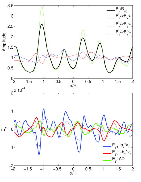
Figure 8.— Equivalence of the top right and bottom left panels of Figure 6, but for run AD-4-64.

AD is generally thought to be a diffusive process, which tends to reduce the magnetic field strength by smoothing out the field gradients. However, unlike Ohmic resistivity, AD is highly anisotropic. It also preserves magnetic field topology since it represents ion-neutral drift without breaking field lines. Brandenburg & Zweibel (1994) demonstrated that AD can in fact lead to the formation sharp magnetic structures, especially near magnetic nulls. This dramatic effect was attributed to two reasons. First, magnetic flux drifts downhill along magnetic pressure gradient, and second, reduction of diffusion in weak field regions. They also showed via a 2D example that even without magnetic nulls, sharp current structures can be formed. While the situation is different in our case, stronger concentration of magnetic flux with sharp vertical flux profiles can be considered as another manifestation on the effect of AD in forming sharp magnetic structures. Weaker net vertical field leads to weaker MRI turbulence, allowing the effect of AD to better stand out.

5. Discussions

Our simulation results demonstrate that magnetic flux concentration and enhanced zonal flows are robust outcome of the MRI in the presence of net vertical magnetic flux, at least in shearing-box simulations. We have also tested the results using an adiabatic equation of state with cooling, where we set the cooling time to satisfy $\Omega t_{\rm cool}=1$. We find exactly the same phenomenon as the isothermal case with strong zonal flows of similar amplitudes and strong flux concentration. Magnetic flux concentration in low density regions of the MRI turbulence was also observed in Zhu et al. (2013), where the low density region was carved by a planet. Concentration of magnetic flux enables the planet to open deeper gaps compared with the pure viscous case. Their results further strengthen the notion of magnetic flux concentration as a generic outcome of the MRI turbulence.

In broader contexts, the interaction of an external magnetic field with turbulence has been studied since the 1960s. Observations of the solar surface show that magnetic flux is concentrated into discrete and intermittent flux tubes with intricate topology, where the field is above equipartition strength to suppress convection. They are separated by convective cells with very little magnetic flux. It is well understood, both theoretically and numerically, that in a convective medium, magnetic flux is expelled from regions of closed streamlines, and concentrates into flux tubes in between the convective cells (e.g., Parker, 1963; Galloway & Weiss, 1981; Nordlund et al., 1992). In the interstellar medium, concentration of magnetic flux in MHD turbulence has also been suggested (Vishniac, 1995; Lazarian & Vishniac, 1996), via a process which they referred to as turbulent pumping. Our findings are in several aspects different from the formation of flux tubes. For example, the distribution of mean vertical magnetic field is quasi-axisymmetric rather than patchy. Also, the level of concentration is modest, with mean vertical field typically weaker than the turbulent field, and the overall distribution of magnetic energy is approximately uniform. Nevertheless, our findings add to the wealth of the flux concentration phenomena, and deserve more detailed studies in the future.

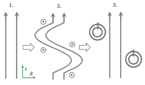
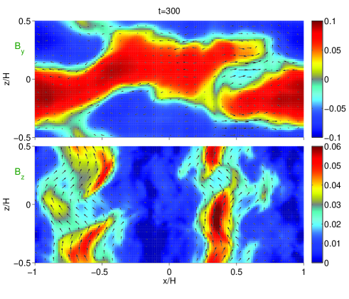
Figure 9.— Top: schematic illustration of a possible mechanism for magnetic flux concentration due to the MRI, where the bold lines represent magnetic field lines. See explanation in Section 5.1. Bottom: a snapshot at $t=300\Omega^{-1}$ from run AD-2-64 showing the azimuthally averaged toroidal (up) and vertical (down) magnetic fields. Arrows indicate the azimuthally averaged in-plane velocity field (up) and magnetic field (down).

5.1. A Possible Physical Picture

Here we describe a possible physical scenario for magnetic flux concentration in the MRI turbulence. It is schematically illustrated on the top panel of Figure 9, which is divided into three stages.

We consider the unstable axisymmetric linear MRI modes in the presence of net vertical magnetic field (stage 1), so-called the “channel flows”. The channel flows exhibit as two counter-moving planar streams, and are found to be exact even in the non-linear regime (Goodman & Xu, 1994). The vertical fields are advected by the streams to opposite radial directions, generating radial fields. The radial fields further generate toroidal fields due to the shear. As a result, oppositely directed radial and toroidal fields are produced and grow exponentially across each stream (stage 2). Eventually, the growth is disrupted by parasitic instabilities or turbulence (Pessah & Goodman, 2009; Latter et al., 2009), effectively leading to enhanced reconnection of such strongly amplified, oppositely directed horizontal fields around each stream. The outcome is represented by two field loops in stage 3. Eventually, these loops are dissipated, and we are back in stage 1.

In the picture above, the material in the loop (stage 3) is originally threaded by net vertical flux. However, due to reconnection, material is pinched off from the original vertical field lines. Therefore, the mass-to-flux ratio in these field lines decreases. In other words, magnetic flux is effectively concentrated into low-density regions. This mechanism resembles the idea of turbulent pumping (Vishniac, 1995; Lazarian & Vishniac, 1996), but relies on the specific properties of the MRI. In brief, the reconnection process following the development of the channel flows effectively pumps out the gas originally threaded by vertical field lines, which results in magnetic flux concentration.

As we have briefly discussed in Section 2.1, the evolution of the MRI shows recurrent bursty behaviors characteristic of discrete channel flows on large scales, followed by rapid dissipation. The overall behaviors are qualitatively similar to the cyclic picture outlined above. A more detailed study carried out by Sano & Inutsuka (2001) lends further support to this picture.

In the presence of strong AD, the above picture is more easily visualized since in the flux-concentrated shells, mean vertical field dominates turbulent field. In the bottom panels of Figure 9, we show a snapshot of azimuthally averaged field quantities from our run AD-2-64. We see that the flux-concentrated shells (at both $x\sim-0.7H$ and $x\sim 0.4H$) show clear signature of sinusoidal-like variations in $z$, indicating the development of channel flows. Given the mean vertical field strength with $\beta_{0}=6400$, the net vertical field in the flux-concentrated shells can be 2-4 times stronger, with $\beta_{z}\sim 400-1600$. The corresponding most unstable wavelength is about $0.5-1H$, consistent with observed features. In the upper panel, we see that toroidal fields are amplified to relatively strong levels ($\beta_{y}\sim 100$). Oppositely directed toroidal fields are separated by sharp current sheets, ready for reconnection to take place. Also, the location of the current sheets approximately coincides with the location where radial field in the channel mode changes sign, consistent with expectations.

Admittedly, the saturated state of the MRI turbulence, especially in the ideal MHD case, contains a hierarchy of scales where the processes described above may be taking place. The final result would be a superposition of loop formation and reconnection at all scales. The simple picture outlined here is only meant to be suggestive. More detailed studies are essential to better understand the physical reality of magnetic flux concentration in the MRI turbulence.

5.2. Implications for Magnetic Flux Transport

The properties of the MRI turbulence strongly depend on the amount of net vertical magnetic flux threading the disk (Hawley et al., 1995; Bai & Stone, 2013a). Therefore, one key question in understanding the physics of accretion disks is whether they possess (or how they acquire) net vertical magnetic flux, and how magnetic flux is transported in the disks.

Conventional studies on magnetic flux transport generally treat turbulent diffusivity as an isotropic resistivity. Balancing viscous accretion and isotropic turbulent diffusion, it is generally recognized that for magnetic Prandtl number of order unity (appropriate for the MRI turbulence e.g., Guan & Gammie, 2009; Lesur & Longaretti, 2009; Fromang & Stone, 2009), magnetic flux tends to diffuse outward for thin accretion disks (Lubow et al., 1994; Guilet & Ogilvie, 2012; Okuzumi et al., 2014).

Our results indicate, at least for thin disks (where the shearing-sheet approximation is valid), that the distribution of magnetic flux in accretion disks is likely non-uniform. Spruit & Uzdensky (2005) showed that if magnetic flux distribution is patchy, inward dragging of magnetic flux can be much more efficient because of reduced outward diffusion and enhanced angular momentum loss on discrete patches. While in our study, magnetic flux concentrates into quasi-axisymmetric shells rather than discrete bundles, we may expect similar effects to operate as a way to help accretion disks capture and retain magnetic flux.

Given the highly anisotropic nature of the MRI turbulence, our results also suggest that it is important to consider the full turbulent diffusivity/conductivity tensor in the study of magnetic flux transport. While the full behavior of this tensor is still poorly known, our results have already highlighted its potentially dramatic effect in magnetic flux evolution. Additionally, magnetic flux evolution can also be strongly affected by global effects, which requires careful treatment of disk vertical structure, as well as properly incorporating various radial gradients that are ignored in shearing-box (Beckwith et al., 2009; Guilet & Ogilvie, 2014).

5.3. Zonal Flow and Pressure Bumps

Our results suggest that magnetic flux concentration and zonal flows are intimately connected. In the context of global disks, radial variations of concentrated and diluted mean vertical field lead to variations of the Maxwell stress or effective viscosity $\nu$. Steady state accretion demands $\nu\Sigma={\rm const}$ (Pringle, 1981). Correspondingly, the radial profile of surface density (hence midplane gas density) is likely non-smooth. The density/pressure variations drive zonal flows as a result of geostrophic force balance. Therefore, the enhanced zonal flows reported in stratified shearing-box simulations with net vertical magnetic flux (Simon & Armitage, 2014; Bai, 2014) are likely a real feature in global disks.

In PPDs, the radial pressure profile is crucial for the growth and transport of dust grains (e.g., Birnstiel et al., 2010), the initial stage of planet formation. Planetesimal formation via the streaming instability favors regions with small radial pressure gradient (Johansen et al., 2007; Bai & Stone, 2010). Sufficiently strong pressure variations may even reverse the background pressure gradient in localized regions to create pressure bumps, which are expected to trap particles or even planets (e.g., Kretke & Lin, 2012). Numerical modelings indicate that such pressure bumps are needed in the outer region of PPDs to prevent rapid radial drift of millimeter sized grains (Pinilla et al., 2012).

Realistic stratified global disk simulations with net vertical magnetic flux is numerically difficult and the results can be affected by boundary conditions. Keeping the potential caveats in mind, radial variations of surface density and Maxwell stress are present in the recent global stratified simulations by Suzuki & Inutsuka (2014), and pressure bumps are also observed in some of their runs. Long-lived zonal flows as particle traps are also seen in the recent global unstratified simulations by Zhu et al. (2014). Therefore, we speculate that because of strong magnetic flux concentration, enhanced zonal flows have the potential to create pressure bumps in the outer regions of PPDs.

6. Conclusions

In this work, we have systematically studied the phenomenon of magnetic flux concentration using unstratified shearing-box simulations. In the presence of net vertical magnetic field, the non-linear evolution of the MRI generates enhanced level of zonal flows, which are banded quasi-axisymmetric radial density variations with geostrophic balance between radial pressure gradient and the Coriolis force. We find that vertical magnetic flux strongly concentrates toward the low density regions of the zonal flow, where the mean vertical field can be enhanced by a factor of $\sim 2$. High density regions of the zonal flow has much weaker or even zero mean vertical field.

In ideal MHD, we find that strong magnetic flux concentration and zonal flow occur when the radial domain size $L_{x}$ reaches $\sim 4H$. The typical length scale of magnetic flux concentration is $\sim 2H$, but the general behaviors of flux concentration do not show clear sign of convergence with increasing simulation box size up to $L_{x}=16H$. In non-ideal MHD with strong ambipolar diffusion (AD), magnetic flux concentrates into thin shells whose width is typically less than $\sim 0.5H$. AD facilitates flux concentration by sharpening the magnetic flux profiles, especially when net vertical flux is weak. The properties of the system converge when the radial domain size reaches or exceeds $\sim 2H$.

Concentration of magnetic flux is a consequence of anisotropic turbulent diffusivity of the MRI. At the saturated state, a turbulent resistivity tends to smear out concentrated magnetic flux. This is balanced by an anti-diffusion effect resulting from a correlation of $\overline{v_{z}B_{x}}$, which has the analogy to the microscopic Hall effect. In addition, a correlation of $\overline{v_{z}B_{y}}$ yields a radial electric field, mimicking the classical Hall effect. We provide a phenomenological description that reasonably fits the simulation results. The physical origin of magnetic flux concentration may be related to the recurrent development of channel flows followed by enhanced magnetic reconnection, a process which reduces the mass-to-flux ratio in localized regions.

Systematic studies of turbulent diffusivities in the presence of net vertical magnetic flux are crucial to better understand the onset of magnetic flux concentration, together with its saturation amplitude. They are also important for understanding magnetic flux transport in general accretion disks. Association of magnetic flux concentration with zonal flows also has important consequences on the structure and evolution of PPDs. This relates to many aspects of planet formation, especially on the trapping of dust grains and planetesimal formation. In the future, global stratified simulations are essential to provide a realistic picture on the distribution and transport of magnetic flux, as well as global evolution of accretion disks.

References

- Bai (2011a) Bai, X.-N. 2011a, ApJ, 739, 50
- Bai (2011b) —. 2011b, ApJ, 739, 51
- Bai (2013) —. 2013, ApJ, 772, 96
- Bai (2014) —. 2014, ApJ, submitted
- Bai & Stone (2010) Bai, X.-N. & Stone, J. M. 2010, ApJ, 722, L220
- Bai & Stone (2011) —. 2011, ApJ, 736, 144
- Bai & Stone (2013a) —. 2013a, ApJ, 767, 30
- Bai & Stone (2013b) —. 2013b, ApJ, 769, 76
- Balbus & Hawley (1991) Balbus, S. A. & Hawley, J. F. 1991, ApJ, 376, 214
- Beckwith et al. (2009) Beckwith, K., Hawley, J. F., & Krolik, J. H. 2009, ApJ, 707, 428
- Birnstiel et al. (2010) Birnstiel, T., Dullemond, C. P., & Brauer, F. 2010, A&A, 513, A79+
- Blackman et al. (2008) Blackman, E. G., Penna, R. F., & Varnière, P. 2008, New Astronomy, 13, 244
- Bodo et al. (2008) Bodo, G., Mignone, A., Cattaneo, F., Rossi, P., & Ferrari, A. 2008, A&A, 487, 1
- Brandenburg & Zweibel (1994) Brandenburg, A. & Zweibel, E. G. 1994, ApJ, 427, L91
- Chapman et al. (2013) Chapman, N. L., Davidson, J. A., Goldsmith, P. F., Houde, M., Kwon, W., Li, Z.-Y., Looney, L. W., Matthews, B., Matthews, T. G., Novak, G., Peng, R., Vaillancourt, J. E., & Volgenau, N. H. 2013, ApJ, 770, 151
- Chiang & Murray-Clay (2007) Chiang, E. & Murray-Clay, R. 2007, Nature Physics, 3, 604
- Davis et al. (2010) Davis, S. W., Stone, J. M., & Pessah, M. E. 2010, ApJ, 713, 52
- Dittrich et al. (2013) Dittrich, K., Klahr, H., & Johansen, A. 2013, ApJ, 763, 117
- Fleming et al. (2000) Fleming, T. P., Stone, J. M., & Hawley, J. F. 2000, ApJ, 530, 464
- Flock et al. (2012) Flock, M., Henning, T., & Klahr, H. 2012, ApJ, 761, 95
- Fromang & Stone (2009) Fromang, S. & Stone, J. M. 2009, A&A, 507, 19
- Galloway & Weiss (1981) Galloway, D. J. & Weiss, N. O. 1981, ApJ, 243, 945
- Goodman & Xu (1994) Goodman, J. & Xu, G. 1994, ApJ, 432, 213
- Guan & Gammie (2009) Guan, X. & Gammie, C. F. 2009, ApJ, 697, 1901
- Guilet & Ogilvie (2012) Guilet, J. & Ogilvie, G. I. 2012, MNRAS, 424, 2097
- Guilet & Ogilvie (2014) —. 2014, MNRAS, 441, 852
- Hawley (2001) Hawley, J. F. 2001, ApJ, 554, 534
- Hawley et al. (1995) Hawley, J. F., Gammie, C. F., & Balbus, S. A. 1995, ApJ, 440, 742
- Hawley et al. (2011) Hawley, J. F., Guan, X., & Krolik, J. H. 2011, ApJ, 738, 84
- Hull et al. (2014) Hull, C. L. H., Plambeck, R. L., Kwon, W., Bower, G. C., Carpenter, J. M., Crutcher, R. M., Fiege, J. D., Franzmann, E., Hakobian, N. S., Heiles, C., Houde, M., Hughes, A. M., Lamb, J. W., Looney, L. W., Marrone, D. P., Matthews, B. C., Pillai, T., Pound, M. W., Rahman, N., Sandell, G., Stephens, I. W., Tobin, J. J., Vaillancourt, J. E., Volgenau, N. H., & Wright, M. C. H. 2014, ApJS, 213, 13
- Johansen et al. (2007) Johansen, A., Oishi, J. S., Low, M.-M. M., Klahr, H., Henning, T., & Youdin, A. 2007, Nature, 448, 1022
- Johansen et al. (2009) Johansen, A., Youdin, A., & Klahr, H. 2009, ApJ, 697, 1269
- Johnson et al. (2008) Johnson, B. M., Guan, X., & Gammie, C. F. 2008, ApJS, 177, 373
- Kretke & Lin (2012) Kretke, K. A. & Lin, D. N. C. 2012, ApJ, 755, 74
- Kunz & Lesur (2013) Kunz, M. W. & Lesur, G. 2013, MNRAS, 434, 2295
- Latter et al. (2009) Latter, H. N., Lesaffre, P., & Balbus, S. A. 2009, MNRAS, 394, 715
- Lazarian & Vishniac (1996) Lazarian, A. & Vishniac, E. 1996, in Astronomical Society of the Pacific Conference Series, Vol. 97, Polarimetry of the Interstellar Medium, ed. W. G. Roberge & D. C. B. Whittet, 537
- Lesur & Longaretti (2007) Lesur, G. & Longaretti, P. 2007, MNRAS, 378, 1471
- Lesur & Longaretti (2009) Lesur, G. & Longaretti, P.-Y. 2009, A&A, 504, 309
- Longaretti & Lesur (2010) Longaretti, P. & Lesur, G. 2010, A&A, 516, A51+
- Lubow et al. (1994) Lubow, S. H., Papaloizou, J. C. B., & Pringle, J. E. 1994, MNRAS, 267, 235
- Masset (2000) Masset, F. 2000, A&AS, 141, 165
- Noble et al. (2010) Noble, S. C., Krolik, J. H., & Hawley, J. F. 2010, ApJ, 711, 959
- Nordlund et al. (1992) Nordlund, A., Brandenburg, A., Jennings, R. L., Rieutord, M., Ruokolainen, J., Stein, R. F., & Tuominen, I. 1992, ApJ, 392, 647
- Okuzumi et al. (2014) Okuzumi, S., Takeuchi, T., & Muto, T. 2014, ApJ, 785, 127
- Parker (1963) Parker, E. N. 1963, ApJ, 138, 552
- Pessah & Goodman (2009) Pessah, M. E. & Goodman, J. 2009, ApJ, 698, L72
- Pinilla et al. (2012) Pinilla, P., Birnstiel, T., Ricci, L., Dullemond, C. P., Uribe, A. L., Testi, L., & Natta, A. 2012, A&A, 538, A114
- Pringle (1981) Pringle, J. E. 1981, ARA&A, 19, 137
- Sano & Inutsuka (2001) Sano, T. & Inutsuka, S.-i. 2001, ApJ, 561, L179
- Shi et al. (2010) Shi, J., Krolik, J. H., & Hirose, S. 2010, ApJ, 708, 1716
- Simon & Armitage (2014) Simon, J. B. & Armitage, P. J. 2014, ApJ, 784, 15
- Simon et al. (2013) Simon, J. B., Bai, X.-N., Armitage, P. J., Stone, J. M., & Beckwith, K. 2013, ApJ, 775, 73
- Simon et al. (2012) Simon, J. B., Beckwith, K., & Armitage, P. J. 2012, MNRAS, 422, 2685
- Simon et al. (2009) Simon, J. B., Hawley, J. F., & Beckwith, K. 2009, ApJ, 690, 974
- Spruit & Uzdensky (2005) Spruit, H. C. & Uzdensky, D. A. 2005, ApJ, 629, 960
- Steinacker & Papaloizou (2002) Steinacker, A. & Papaloizou, J. C. B. 2002, ApJ, 571, 413
- Stone & Gardiner (2010) Stone, J. M. & Gardiner, T. A. 2010, ApJS, 189, 142
- Stone et al. (2008) Stone, J. M., Gardiner, T. A., Teuben, P., Hawley, J. F., & Simon, J. B. 2008, ApJS, 178, 137
- Stone et al. (1996) Stone, J. M., Hawley, J. F., Gammie, C. F., & Balbus, S. A. 1996, ApJ, 463, 656
- Suzuki & Inutsuka (2014) Suzuki, T. K. & Inutsuka, S.-i. 2014, ApJ, 784, 121
- Uribe et al. (2011) Uribe, A. L., Klahr, H., Flock, M., & Henning, T. 2011, ApJ, 736, 85
- Vishniac (1995) Vishniac, E. T. 1995, ApJ, 446, 724
- Zhu et al. (2014) Zhu, Z., Stone, J. M., & Bai, X.-N. 2014, ArXiv e-prints
- Zhu et al. (2013) Zhu, Z., Stone, J. M., & Rafikov, R. R. 2013, ApJ, 768, 143