The Structure, Dynamics and Star Formation Rate of the Orion Nebula Cluster

Abstract

The spatial morphology and dynamical status of a young, still-forming stellar cluster provide valuable clues on the conditions during the star formation event and the processes that regulated it. We analyze the Orion Nebula Cluster (ONC), utilizing the latest censuses of its stellar content and membership estimates over a large wavelength range. We determine the center of mass of the ONC, and study the radial dependence of angular substructure. The core appears rounder and smoother than the outskirts, consistent with a higher degree of dynamical processing. At larger distances the departure from circular symmetry is mostly driven by the elongation of the system, with very little additional substructure, indicating a somewhat evolved spatial morphology or an expanding halo. We determine the mass density profile of the cluster, which is well fitted by a power law that is slightly steeper than a singular isothermal sphere. Together with the ISM density, estimated from average stellar extinction, the mass content of the ONC is insufficient by a factor $\sim 1.8$ to reproduce the observed velocity dispersion from virialized motions, in agreement with previous assessments that the ONC is moderately supervirial. This may indicate recent gas dispersal. Based on the latest estimates for the age spread in the system and our density profiles, we find that, at the half-mass radius, 90% of the stellar population formed within $\sim 5$–$8$ free-fall times ($t_{\rm ff}$). This implies a star formation efficiency per $t_{\rm ff}$ of $\epsilon_{\rm ff}\sim 0.04$–$0.07$, i.e., relatively slow and inefficient star formation rates during star cluster formation.

1. Introduction

The majority of stars, perhaps including our Sun, have their origin in clusters (Lada & Lada, 2003; Gutermuth et al., 2009). Thus understanding the formation of star clusters is important both for their role as the basic building blocks of galactic stellar populations and for being the birth environments of most planetary systems.

In spite of this importance, some basic questions about star cluster formation are still debated, including whether it is dynamically fast (Elmegreen, 2000, 2007; Hartmann & Burkert, 2007) or slow (Tan et al. 2006 [TKM06]; Nakamura & Li 2007, 2014) process: in essence, is the duration of star cluster formation similar to a dynamical time (similar to the free-fall time) of the natal gas clump or is it much longer? The latter scenario would be consistent with some theoretical expectations of relatively low star formation efficiency per free-fall time in turbulent and/or magnetized gas (Krumholz & McKee, 2005; Padoan & Nordlund, 2011) and with turbulence being maintained by self-regulated protostellar outflow feedback (Nakamura & Li, 2007, 2014).

As discussed by TKM06, there are several ways to try and distinguish between these scenarios, including considering the morphologies of gas clumps, the morphologies of embedded stars, assessing the momentum flux of protostellar outflows, looking at the age spreads of pre-main sequence stars and the ages of dynamical ejection events. By considering these factors, especially in the context of the relatively nearby (414 pc, Menten et al. 2007) and massive ($\sim$ few thousand $M_{\odot}$, Hillenbrand & Hartmann 1998) Orion Nebula Cluster (ONC), TKM06 concluded the duration of star cluster formation, as defined by $t_{\rm form,90}$, the time to form 90% of a cluster’s stars, was $\geq 4\bar{t}_{\rm dyn}\simeq 8\bar{t}_{\rm ff}$, where $t_{\rm dyn}=R/\sigma$, $R$ being the local radius, $\sigma$ being the 1D velocity dispersion and the bar indicating this is the mass-weighted average of $t_{\rm dyn}$ over the region containing the stars that count towards $t_{\rm form,90}$. The free-fall time is defined via $t_{\rm ff}\equiv[3\pi/(32G\rho)]^{1/2}$, where $\rho$ is the volume density, and for a virialized cloud with $\alpha_{\rm vir}\equiv 5\sigma^{2}R/(GM)\sim 1$ (Bertoldi & McKee, 1992), we have $t_{\rm ff}\sim 0.5t_{\rm dyn}$. For the ONC, TKM06 adopted $M=4600\>M_{\odot}$, $\Sigma=M/(\pi R^{2})=0.12\>{\rm g\>cm^{-2}}$, $R=1.60$ pc, so that $t_{\rm dyn}=7\times 10^{5}$ yr and $t_{\rm ff}=3.5\times 10^{5}$ yr. They assumed star formation, which is still on-going, has a duration $t_{\rm form,90}\geq 3$ Myr.

The estimate of $t_{\rm form,90}$ in the ONC is measured most directly via age spreads of pre-main sequence stars, as revealed by spreads of luminosity in the HR diagram in comparison with stellar evolutionary models. However, other factors can also lead to this luminosity spread, including the difficulty in assigning stellar parameters to individual stars (Da Rio et al., 2010b; Reggiani et al., 2011) and, episodic protostellar accretion (Baraffe et al., 2009, 2012; Hosokawa et al., 2011). Da Rio et al. (2014) examined the problem of age spread in the Orion Nebula Cluster (ONC) and concluded, from independent constraints that there is an intrinsic age spread of $\sim 1.34$ Myr as defined by 1$\sigma$ dispersion in ages. Assuming a log-normal age distribution or a constant SFR in time, this leads to $t_{\rm form,90}\geq 4.1,4.2$ Myr, respectively.

In this paper we re-visit questions of the timescale of star cluster formation as exemplified by the ONC. First we consider the spatial structure of stars in the cluster to investigate the TKM06 assertion of progressively smoother stellar distributions (smaller amounts of substructure) as a cluster ages. We do this by examining angular substructure in annuli as a function of radius (adapting methods used by Gutermuth et al. 2005). The theoretical expectation is that center of the cluster, being dynamically older because of its shorter local dynamical time but similar age spread (Da Rio et al., 2012) has a smoother distribution of stars, since any initial substrucure has had more dynamical timescales to be erased. This analysis first requires a careful assessment of the location of the center of mass of the ONC; and then analysis of radial variation of angular substructure. This is presented in §3.

Then in §4, utilizing the latest mass and age estimates of the stars in the ONC and allowing for contributions of gas to the total mass, we examine the mass density profile of the ONC. Using literature measurements for the velocity dispersion we refine previous assessment concerning the ONC dynamical equilibrium. In §5 we compute the ratio of $t_{\rm form,90}$ with $t_{\rm ff}$ as a function of radius in the cluster. Together with the latest estimate of the age spread in the system, this allows us to measure the star formation efficiency per free-fall time, $\epsilon_{\rm ff}=0.9\epsilon_{*}t_{\rm ff}/t_{\rm form,90}$, where $\epsilon_{*}\equiv M_{*}/M_{\rm tot}=\rho_{*}/\rho_{\rm tot}$. We are able to measure $\epsilon_{\rm ff}$ both locally as a function of projected radius (making the simplifying approximation that projected radius is 3D radius) and as an average interior to a given radius.

2. The stellar catalogs

We assemble catalogs of stellar positions and properties in the ONC from the literature.

We first compiled a sample of all sources with available stellar parameters, including spectroscopically determined $T_{\rm eff}$ and $\log L$, as well as (model dependent) ages and masses. In this context, the H-R diagram of Da Rio et al. (2012) represents the latest update; it is obtained combining spectral types from either spectroscopy or narrow-band photometry with optical multi-band photometry to measure the reddening towards each source and calculate bolometric luminosities. This sample covers a field of view of about $\sim 40$^′$\times 40$^′ on the Orion Nebula centered south-west of the Trapezium, and is nearly complete for $A_{V}<5$ mag down to the H-burning limit, while also extending into the substellar regime. Sources flagged as probable non-member contaminants in Da Rio et al. (2012) have been excluded from the catalog. We further extended this catalog adding new spectral types from Hillenbrand et al. (2013); for these stars the extinction, $A_{V}$, and thus $\log L$, has been assigned using $BVI$ photometry from Da Rio et al. (2010a) and adopting the same analysis technique as in that work. Also, since Da Rio et al. (2012) was incomplete towards the massive end of the population, due to saturation of their photometry, we added all of such missing sources adopting the stellar parameters from the Hillenbrand (1997) catalog. Last, the masses of the Trapezium stars have been adjusted to account for their multiplicity, using estimates of masses for each multiple system from Grellmann et al. (2013). The final catalog of optically determined stellar parameters contains 1597 sources.

We also constructed a catalog of near-infrared (NIR) photometry. We based this on the $JHK$ catalog from Robberto et al. (2010), which covers an area slightly larger than that of our optical photometry, and has a very deep detection limit ($3\sigma$ detection at $J=19.5$ mag, $H=18$ mag), reaching down to planetary masses, and nearly complete for $A_{V}<20$ mag for stellar objects. We complement this sample for the saturated bright end using data from the Two Micron All Sky Survey (2MASS, Skrutskie et al. 2006). We also collected the mid-infrared Spitzer survey in Orion from Megeath et al. (2012). This catalog provides stellar fluxes from the $J$ band to 24 $\rm\mu m$, and includes the classification of sources showing infrared excess from dusty stellar surroundings (either disks or protostellar objects). This was based on the multi wavelength, near- and mid-infrared criteria described in Gutermuth et al. (2009). Last, we used the X-ray source catalog of Getman et al. (2005a) from the Chandra Orion Ultradeep Project (COUP), and rejected sources flagged by Getman et al. (2005b) as non members of the Orion population (nebular shocks, extragalactic sources, or unconfirmed members).

All these catalogs have been cross-matched, and the resulting dataset limited to the sky area covered by the optical data. The X-ray sample alone has a smaller coverage than the other datasets, complete up to $\sim 0.11$^∘ from the Trapezium; all the other catalogs extend to a radius of $\sim 0.2$^∘ at any position angle. This corresponds to a projected distance of $\sim 1.4$ pc from the center, assuming a distance for the ONC of 414 pc (Menten et al., 2007).

Despite the richness of this dataset, it is difficult to precisely isolate the ONC population, as all these samples alone suffer from some combination of incompleteness or contamination from non-members. The optical catalog of stellar parameters is naturally limited by dust extinction, which is also not spatially uniform. The NIR photometry is nearly complete at high extinctions, lacking only a minor fraction of young members in the heavily embedded OMC-1 cloud, as well as protostellar objects in the vicinity of the Kleinmann-Low (KL) nebula; however, this sample suffers significant contamination from Galactic field populations, which increases towards low stellar luminosities. The X-ray sample is not limited significantly by extinction, but suffers incompleteness at low stellar masses ($M<0.2$ M_⊙) and in the Trapezium cluster due confusion from the broad tails of the PSF of the bright objects. Last, the Spitzer survey also suffers from incompleteness in the detection at low masses, and confusion in the core due to the lower angular resolution compared to the other samples.

In the following sections, we will assume the combination of the optical parameter and the X-ray sample as representative of the spatial structure of the ONC. This joint sample, although somewhat incomplete, is virtually immune from field contamination and not biased by patchy extinction. The remaining sources in the IR samples will be considered when assessing the total stellar mass and its radial density profile.

3. The Structure of the ONC

3.1. The Center of the ONC

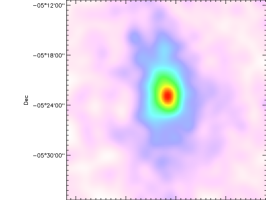
Figure 1.— Left panel: ONC stellar density map, limited to an angular box of 0.4^∘ (2.9 pc) centered on $\theta^{1}C$ for our sample of optical and X-ray members. Middle panel: The catalog of positions; symbols denote stellar mass if known, crosses indicate X-ray sources with unknown mass. The circle delimits the aperture of radius 0.11^∘ (0.9 pc) fully contained within the COUP X-ray field of view. The orange box delimits the area shown in the Right panel. Right panel: The Trapezium region; the red arrows indicate the moving center of mass of the population decreasing the considered aperture from the entire catalog (red diamond) to the COUP FOV aperture (red square) to the central radius 0.01^∘ (0.072 pc) (red star). Blue and green stars mark, respectively, the shift of the final result when excluding $\theta^{1}$C from the sample, or including it but as if it were located at the position of the ejection event proposed by Chatterjee & Tan (2012) (orange plus symbol).

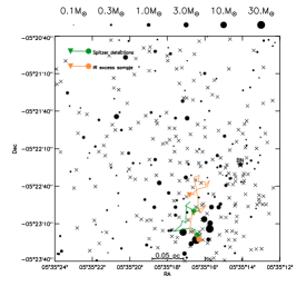
Figure 2.— Same as Figure 1, but tracing the displacement of ONC center of mass assuming different samples. Left panel: the COUP X-ray sample, and the same considering separately lightly and heavily embedded sources. Middle panel: the NIR photometry, considering all detections, detections above the CMD threshold dividing stellar members from BD and contaminants, and the latter divided in 2 extinction samples. Right panel: the Spitzer detections sample, and the same limited to sources showing infrared excess from their SED. In every panel the triangles denote the “starting” positions from the largest aperture, and the circles the final centers at small scales.

It is well established that the massive stars of the Trapezium cluster lie roughly at the center of the stellar population of the ONC; here we aim to better characterize the actual position of the center of mass of the population. Hillenbrand & Hartmann (1998), based on ellipse fitting on isophotes on an optical+NIR stellar density map found the center of the stellar positions to be located $\sim 25$^′′ north of $\theta^{1}$C and slightly to the west, just outside the Trapezium cluster. Feigelson et al. (2005), based on the COUP X-ray sample, noted that the heavily embedded sources ($\log N_{\rm H}>22$ cm^-2, corresponding to $A_{V}\gtrsim 6$ mag) are systematically offset to the north-west of the Trapezium compared to the lightly obscured members. This, however, may be in part due to the spatial variations of extinction, which are present in the ONC at all column densities.

We have considered the merged catalog of available optical stellar parameters with X-ray members to evaluate the position of the center of mass of the ONC. The collected census counts 2228 members in total, or 1901 sources within the square area of size 0.4^∘ centered on $\theta^{1}$C common to all catalogs, to which we restrict our analysis. About 2/3 of the stars in this sample have a mass estimate from optical studies; the remaining are X-ray members with no mass estimate. We assign to these sources a mass $M=0.5M_{\odot}$, i.e., the mean mass of the Kroupa (2001) initial mass function. In fact, as mentioned, the X-ray sample is incomplete below 0.2$M_{\odot}$, so its mean stellar mass should be higher; on the other hand all the massive stars in the ONC have optical parameters, so this lowers the mean mass of the X-ray sample with no available mass estimate. The stellar positions included in our final catalog of optical and X-ray sources are shown in Figure 1, left and center panels; the circle of radius 0.11^∘ in the center panel delimits the maximum aperture fully contained in the X-ray field of view.

The center of the ONC has been computed in an iterative way, from large to small scales: first we considered the largest circular aperture contained in the whole area shown in Figure 1 and determined its center of mass. This has been then used as a center of a slightly smaller circular aperture, where the sample has been limited to, in order to re-derive its center of mass. The procedure has been iterated to progressively smaller circles, down to $\sim$0.6^′, each time using as the aperture center the center of mass of the previous one. Figure 1, right panel shows the displacement of the center of mass from largest area, to the X-ray complete aperture and then to the smallest aperture. We find that at large apertures the center of mass is displaced $\sim 30$^′′ (0.05 pc) north of the $\theta^{1}$C and outside the Trapezium, in agreement with previous works. When we reduce the aperture to sample the center at smaller scales, this progressively moves inside the Trapezium, indicating some degree of asymmetry at different scales. We will consider the latter center, located at $\alpha_{\rm J2000}=05^{h}~{}35^{m}~{}16.26^{s}$; $\delta_{\rm J2000}=-05\hbox{${}^{\circ}$}~{}23$^′$~{}16.4$^′′  as our bona-fide center of the ONC.

We have tested how this result is sensitive to the assumed value of stellar mass for uncharacterized X-ray sources, and find no displacement (less than 1^′′) if this value is lowered to $M_{\rm X-ray}=0.3\>M_{\odot}$.

Finally, we note that the local ONC center of mass lies close to the point where, tracking proper motions in reverse, as proposed by Chatterjee & Tan (2012), $\theta^{1}$C and the Becklin-Neugebauer (BN) object were co-located $\sim 4500$ years ago. It is proposed that a strong gravitational slingshot interaction ejected BN into the molecular cloud at $\sim 30\>{\rm km\>s^{-1}}$ with $\theta^{1}$C recoiling in the opposite direction to its current location. Thus, we have recalculated the ONC center of mass both removing $\theta^{1}$C from the sample, or displacing its position to the point of the past interaction. In both cases, as shown in Figure 1, our calculated center of mass moves even closer to the interaction point. This qualitative argument could strengthen the hypothesis of Chatterjee & Tan (2012), as the system of $\theta^{1}$C, the most massive star in the cluster, would tend to settle in the very center of the cluster via gentle interactions with other ONC members. Its current displacement from the ONC center of mass is then explained as a result of its strong interaction with BN. If true, this scenario has the potential to place constraints on the formation time and radial displacement from cluster center of the formation site of $\theta^{1}$C.

3.2. Displacement of the ONC Center

We now study how the center of the ONC, and its variations upon aperture scale, depends on the sample of sources we have adopted. First we aim to test if the incompleteness of our optical and X-ray sample could bias our derived ONC center; second, we look for systematic displacements of the center of the population as a function of dust extinction, which provides some indication of the distribution of stars and gas along the line of sight. Hillenbrand & Hartmann (1998) found no significant variations of the spatial distribution of sources observed in the optical and in the near infrared. Using X-ray derived extinctions, which reach to higher column densities than near infrared photometry, Feigelson et al. (2005) however found the embedded population to be more concentrated to the east of the Trapezium cluster, with over-concentrations aroung the BN/KL region and the OMC-1S region. Feigelson et al. (2005), however, set the division between the lightly and heavily obscured samples at $\log N_{\rm H}=22$ cm^-2 which corresponds to $A_{V}\sim 6$ mag, a value low enough to be sensitive to the non uniformity of the average extinction of the ONC (see, e.g., the extinction maps from Scandariato et al. 2011), rather than a value separating highly embedded members which cannot be detected in the optical or NIR.

We first considered the X-ray sample alone, and converted the column densities $\log N_{\rm H}$ derived from the X-ray spectral analysis of Getman et al. (2005a) into dust extinction $A_{V}$ assuming the relation $N_{\rm H}/A_{V}=1.58\times 10^{21}$ cm^-2 (Vuong et al., 2003) . We then separated the sample in 2 sub samples with $A_{V}<20$ mag and $>20$ mag, and computed the center. This was performed as in §3.1. Figure 2 (left panel) shows that the center of the ONC remains confined inside the Trapezium when considering the sample with up to 20 mag of extinction, which corresponds to $\sim 85\%$ of the population. The remaining small fraction of heavily embedded sources remains spatially centered $\lesssim 0.1$ pc to the northwest of the Trapezium in the direction of the BN/KL region. This is not surprising as the KL region is associated to the densest molecular core within the OMC-1 filament (Johnstone & Bally, 1999; Grosso et al., 2005).

Next, we have computed the center of the ONC adopting the NIR photometric sample. We have separately considered either the entire sample, and that restricted to sources brighter than the reddening vector in the $J$ versus $J-H$ diagram corresponding to a mass of $0.075M_{\odot}$. Robberto et al. (2010) has shown that below this locus in the NIR CMD, roughly corresponding to the substellar mass range, the vast majority of sources are faint field contaminants rather than young brown dwarfs. Figure 2 (middle panel) shows removing or not this faint population of probable contaminants has little effect on the derived center of the ONC. As for the X-ray sample, we divide the NIR catalog according to extinction. This was roughly computed by deredding the $J$ vs $J-H$ CMD on a 2.5 Myr Siess et al. (2000) isochrone. Again, the center of the lightly embedded population is confined within the Trapezium cluster, but this moves north at higher $A_{V}$, at a higher declination than for the X-ray embedded population. This result has two origins: first, the NIR sample is severely limited by dust extinction in the densest BN-KL and OMC-1S regions, whose combined embedded populations (dominated by OMC-1S) would thus shift the center of the obscured population to the south-west; second, at high extinction the NIR catalog from Robberto et al. (2010) has a spatially variable completeness, and all sources with $A_{V}>15$ are located on a stripe around $\delta=-5$^∘18^′, which coincides with the overlapping area between adjacent exposures of the imaging mosaic, and thus has higher effective photometric depth. Such a feature in the spatial completeness therefore biases the center towards the north at high $A_{V}$.

Last, we considered the Spitzer sample; Figure 2 (right panel) shows that its center remains compatible with that of the other catalogs, and does not vary when limiting to sources showing infrared excess emission. This suggests that there are no significant spatial offsets between young members with disks and diskless sources, although their radial profile might not be identical.

3.3. Ellipticity

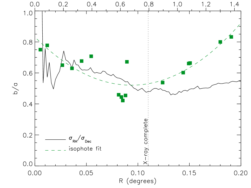
Figure 3.— Axes ratio, $b/a$, of ONC stars. The green squares are the best elliptical fits to isophotes on the ONC map, and trace the local ellipticity. The green dashed line line is a 2^nd order polynomial fit to these results. Black solid line: cumulative flattening of the population in the north-south direction as a function of maximum distance in declination from the center, estimated from the ratio of the positional dispersions in RA and Dec (see text).

The ONC population is known to be elongated in a direction close to north-south, which follows the local filamentary structure of the Orion A molecular cloud (Johnstone & Bally, 1999; Muench et al., 2008). Hillenbrand & Hartmann (1998) fitted ellipses to isophotes on a stellar spatial density map in the ONC, obtaining average ellipticity $e=1-b/a=0.30$, identical for their optical and NIR sample, with a tilt of the major axis at about 10^∘ counterclockwise from the north-south direction.

We remeasure the ellipticity of the ONC considering our catalog of optical parameters and X-ray members as representative of the structure of the cluster. We evaluate both a “local” and a scale dependent “overall” ellipticity. We compute the first in a similar way as in Hillenbrand & Hartmann (1998), we generate a stellar density map, and smooth it with a Gaussian kernel of 36^′′ ($\sim 0.08$ pc). We recompute the tilt of the major axis of the cluster, which from our catalog is only 7^∘, and choose to neglect it as negligible throughout our analysis. We also constrain the center of each fitted ellipse to be our reference ONC center, computed on the same catalog, derived in §3.1.

We also compute a overall ellipticity of the entire ONC population within varying distances from the center. To this end, we proceed in an iterative way: we consider square boxes centered on our ONC center, and compute the ratio between the standard deviations in RA and Dec of the sources contained. If the ratio departs from one, we change the size of the box in RA (generally diminishing it given the north-south elongation of the ONC), and recompute the ratio of the dispersions of the sample contained in this rectangular area. We iterate until the measured ratio of sample standard deviation converges to the ratio of the sides of the box.

The result, in terms of axis ratio $b/a=1-e$ as a function of distance in declination from the center is shown in Figure 3. Our isophote fits show that the core of the cluster is relatively round, and the distribution becomes more elliptical at increasing radii, reaching a value $b/a\sim 0.5$; this is compatible with Hillenbrand & Hartmann (1998)’s results, which were obtained up to a distance (semimajor axis) of 0.14^∘ from the center. At larger distances, however, the cluster becomes again rounder, with a semimajor axes ratio of $\sim 0.8$. The black line in Figure 3 shows the cumulative $b/a$ as a function of radius: its increase at distances from the center ($\gtrsim 0.12$^∘) is more modest since the enclosed stellar content remains dominated by stars in the more elliptical region.

3.4. Angular Substructure

3.4.1 The Angular Dispersion Parameter

Figure 4.— Example of the subdivision of the ONC population in sectors and annuli, assuming circular symmetry (left panel, blue lines), constant ellipticity (center panel, red lines), or radially variable ellipticity (right panel, green lines). The dashed lines show another possible orientation of the sector pattern.

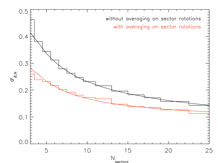
Figure 5.— The measured error, $\sigma_{\delta,N}$, in the angular dispersion parameter, $\delta_{\rm ADP,N}$, versus number of sectors, $N$, from our Monte Carlo simulation, assuming a fixed pattern of sectors for each simulated stellar distribution (black histogram) or averaging $\delta_{\rm ADP,N}$ for the $n_{\rm tot}$ possible rotations of the patters (red histogram). The black line is the analytic prediction for the first from Equation 2, the red line its scaling to match the red histogram.

.

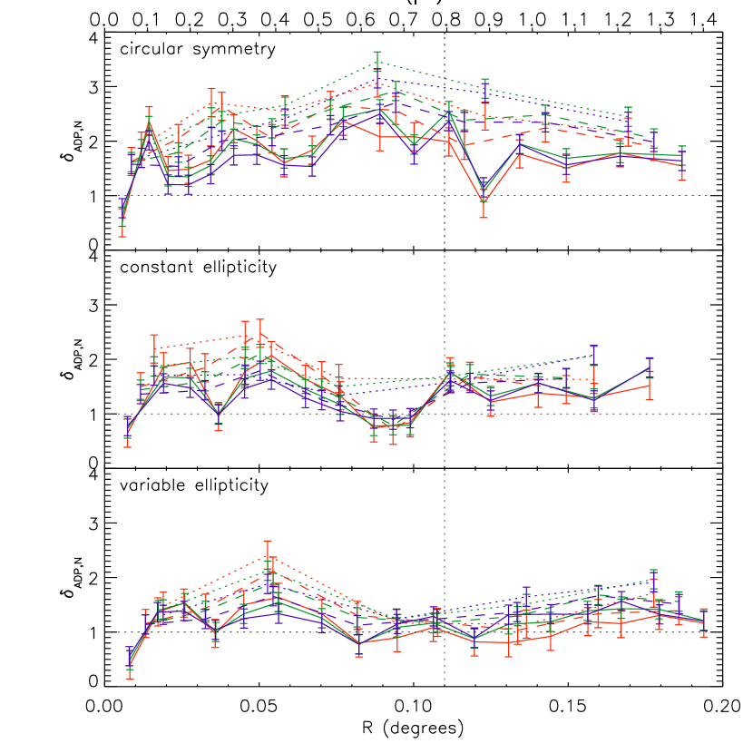
Figure 6.— Angular dispersion of stellar counts in sectors normalized on that expected for Poisson statistics, as measured by the ADP, as a function of radial distance from the center of the selected annuli. Lines corresponds to different numbers sectors and stars per annulus, and for the assumption of circular symmetry as opposed to elliptical symmetry. The vertical dotted line at delimits the X-ray complete sample at $r<0.11$^∘.

We estimate the degree of angular sub-structure in the ONC, or conversely, the smoothness of the stellar distribution, using a technique analogous to the “azimuthal asymmetry parameter” (AAP) defined by Gutermuth et al. (2005). This is based on dividing the spatial stellar distribution in equally sized circular sectors, and comparing the dispersion of the number counts among different sectors with the hypothesis of being drawn from a uniformly random distribution of position angles. Varying the width (or number) of the sectors allows one to probe positional substructure at different azimuthal multipole moments. The radial dependence of the degree of angular substructure can be investigated by further isolating the population within concentric annuli before counting sample numbers within azimuthal sectors.

In addition to radial variation, we will also generalize the AAP of Gutermuth et al. (2005) to account for cluster ellipticity. We thus define a new angular dispersion parameter (ADP), $\delta_{\rm ADP,N}(R)$. For each annulus, the number $n_{i}$ of stars in each $i$-th sector is counted over a total of $N$ sectors; the quantity $\delta_{\rm ADP,N}$ is then defined as follows:

$$\delta_{\rm ADP,N}=\sqrt{\frac{1}{(N-1)\overline{n}}\sum\limits_{i=1}^{N}\big{(}n_{i}-\overline{n})^{2}}=\sqrt{\frac{\sigma^{2}}{\sigma^{2}_{\rm Poisson}}}$$ (1)

where $\sigma$ is the standard deviation of the $n_{i}$ values, $\overline{n}$ is the average of the number of stars per sector in the considered annulus, and $\sigma_{\rm Poisson}$ is the expected standard deviation due to Poisson statistics. When the annuli follow the local or mean elliptical shape of the cluster, we indicate this via $\delta_{\rm ADP,e,N}$ and $\delta_{\rm ADP,\bar{e},N}$, respectively. The ADP simply corresponds to the measured sample standard deviation of counts in sectors normalized on that expected assuming Poisson statistics. Practically, an azimuthal random distribution of stars would produce a measured $\delta_{\rm ADP,N}\sim 1$; in presence of intrinsic cluster sub-structuring, the measured dispersion increases to values $>1$.

Strictly speaking, since the sample variance $\sigma^{2}$ follows a scaled $\chi^{2}$ distribution, as $(N-1)\sigma^{2}/\sigma_{\rm Poisson}^{2}$ follows a $\chi^{2}_{N-1}$ distribution with $N-1$ degrees of freedom, we have that the expected value of $\delta_{\rm ADP,N}^{2}$ is 1 if the stellar distribution is azimuthally random, but the non linearity of the square root in Equation 1 lowers the mean of $\delta_{\rm ADP,N}^{2}$ to $\sim 0.93$ for $N=4$, to $\sim 0.95$ for $N=6$ and to 1 for $N\rightarrow\infty$.

Since $\delta_{\rm ADP,N}$ is a random variable subject to a statistical error, deviations from 1 are expected even for a random distribution of stars. From the relations mentioned above, the standard error in $\delta_{\rm ADP,N}$ will be:

$$\sigma_{\delta,N}=\sqrt{{\rm Var}[\delta_{\rm ADP,N}]}=\sqrt{{\rm Var}\left[\frac{1}{N-1}\chi^{2}_{N-1}\right]},$$ (2)

which does not depend on the number of stars, but on the number of sectors. For a small number of sectors, this error is relatively large: for example $\sigma_{\delta,N}\simeq 0.25$ for 4 sectors and $\simeq 0.17$ for 10 sectors.

A way to lower this error is to decrease the probability of the measured $\delta_{\rm ADP,N}$ deviates from the expected value because of the particular orientation of the sector pattern (e.g., the edge between two contiguous sectors oriented in the north-south direction as shown in Figure 4). Instead, the value of $\delta_{\rm ADP,N}$ can be computed for multiple orientations of the sector pattern and the results averaged. The total number of unique redistributions of $n_{\rm tot}=N\bar{n}$ sources within an annulus among the different sectors obtained by rigid rotations of the sector patter is $n_{\rm tot}$; so we compute $\delta_{\rm ADP,N}$ for each of all these cases and average the $n_{\rm tot}$ results.

We characterize the decrease of $\sigma_{\delta,N}$ due to our averaging process through Monte Carlo simulations. We generate a large number of simulated stellar distributions with random positions within a circular aperture, and estimate the error $\sigma_{\delta,N}$ as the standard deviation of the dispersions measured for each realization. We repeat the experiment changing the the number of stars within the aperture (from 20 to 5000) and the number of sectors. Also, in each case we separately test the cases of measuring $\delta_{\rm ADP,N}$ assuming a fixed pattern of sectors, or performing an average over the $n_{\rm tot}$ possible orientations of the patterns for each simulated distribution. Results show that $\sigma_{\delta,N}$ is independent of $n_{\rm tot}$ also in the latter case. Instead (see Figure 5), the value of $\sigma_{\delta,N}$ when the rotational averaging is performed is lower than that for a fixed sector pattern by an amount that depends on the number of sectors, being from $\sim 30\%$ smaller for 4 sectors and $\sim 20\%$ for more than 20 sectors. In our analysis that follows, we will always adopt the value of $\delta_{\rm ADP,N}$ obtained by averaging over sectors rotations, and the error bar $\sigma_{\delta,N}$ on these derived from our Monte Carlo simulations (red line in Figure 4).

We have established that the statistical uncertainty in $\delta_{\rm ADP,N}$ does not depend on the number of stars, $n_{\rm tot}$, in an annulus or circular aperture. However, if a population of stars is not azimuthally uniform, a given degree of substructure will lead to different values $\delta_{\rm ADP,N}>1$ depending on $n_{\rm tot}$. This is because of the normalization of $\delta_{\rm ADP,N}$ over the expected dispersion for a Poisson distribution: increasing $n_{\rm tot}$ causes the relative expected standard deviation of the star counts in sectors (over the total counts) to decrease. Thus, for a given relative increase in the measured standard deviation of counts produced by substructure, the higher the number of stars, the higher the value of $\delta_{\rm ADP,N}$. Thus, when comparing the measured $\delta_{\rm ADP,N}$ between different star clusters, or different radial bins for the same cluster, or for different assumed samples for the same cluster, the number of sources within an aperture or annulus must be fixed.

Before we analyze the properties of the ADP, $\delta_{\rm ADP,N}$, in the ONC, we briefly characterize the typical ranges of the variation of this parameter between very smooth and highly substructured stellar populations, and in particular consider Globular Clusters (GCs) and the PMS stars in Taurus-Auriga. For the GCs, we adopt the catalogs from the ACS Survey of Galactic Globular Clusters (Sarajedini et al., 2007; Anderson et al., 2008), which includes HST photometry of about 50 GCs. For the Taurus association, we use the census of PMS stars from Kenyon et al. (2008) which includes 383 members. For each GC and for Taurus we derive the center of the cluster as in §3.1, divide the population in circular annuli and sectors, forcing a fixed number of sources within each annulus, and compute $\delta_{\rm ADP,N}$. Then we average the results for multiple annuli in Taurus and all annuli of all GCs. Table 1 shows the results, compared with that obtained in the ONC assuming the optical parameters + X-ray sample, and imposing either 50 or 100 stars per annulus. Such a low number, very small compared to the number of sources in the GCs and also in the ONC, is required to allow a meaningful comparison with the small sample of the Taurus region.

Table 1Average measured dispersion $\delta_{\rm ADP,N}$

50 stars per annulus
	4 sectors	6 sectors	9 sectors
Globular Clusters	0.92	0.95	0.96
ONC	1.39	1.40	1.31
Taurus	2.77	3.01	3.03
100 stars per annulus
	4 sectors	6 sectors	9 sectors
Globular Clusters	0.92	0.95	0.97
ONC	1.80	1.79	1.63
Taurus	2.98	3.52	3.54

Table 1 shows a trend clear in the ADP from the smooth, dynamically old, GCs, where the $\delta_{\rm ADP,N}\simeq 1$ indicates a near random azimuthal distribution of sources (indeed such low values are expected due to the regularization imposed by the global potential of the cluster, while increased values may result from a spread in stellar masses), to the ONC where departures from Poisson smoothness are detected ($d\simeq 1.4$ for 50 stars per annulus, $\delta_{\rm ADP,N}\simeq 1.8$ for 100 stars per annulus), to the substructured distribution in Taurus leading to an azimuthal dispersion up to twice as large as in the ONC. These results highlight the ability of the azimuthal dispersion parameter $\delta_{\rm ADP,N}$ to trace small departures from angular spatial smoothness: another technique such as the minimum spanning tree $Q$ parameter (Cartwright & Whitworth, 2004) is a powerful tracer of substructure for clumpy spatial distributions, but in the ONC ($Q\sim 0.8$) would merely indicate central concentration.

3.4.2 Radial Dependence of the Angular Dispersion Parameter in the ONC

We now look for radial variations in the ADP of the ONC, i.e. $\delta_{\rm ADP,N}(r)$. Also, we account for the ellipticity of the cluster and consider separately 3 assumptions

Circular symmetry

we simply divide the stellar sample in concentric circular annuli in RA and Dec to derive $\delta_{\rm ADP,N}(r)$.

Constant ellipticity

we assume elliptical annuli, with an axes ratio $b/a=0.55$ corresponding to the overall ellipticity we have determined within large apertures ($a>0.1$^∘) from the ONC center (see Figure 3) to derive $\delta_{\rm ADP,\bar{e},N}(r)$. The position angles of the segments separating neighboring sectors are corrected to maintain equal areas within each sector.

Variable ellipticity

we assume the polynomial fit to the best fit isophotes shown in Figure 3, allowing the flattening of subsequent annuli to vary with the distance from the center, to derive $\delta_{\rm ADP,e,N}(r)$. As in the previous case, the edge between neighboring sectors is defined to force the area of all sectors in each annulus to be constant, this produces curved lines separating sectors.

An example of the 3 configurations we explore is shown in Figure 4. As before, we assume the combined sample of optical and X-ray sources.

Figure 6 reports the radial dependence of $\delta_{\rm ADP,N}$ from our ONC stellar sample, for multiple configurations of number of sectors and stars per annulus, as reported in the legend. As anticipated, increasing the number of stars per annulus leads, on average, to a larger measured value of $\delta_{\rm ADP,N}$, whereas we do not detect significant differences in the results changing the number of sectors, i.e., the angular mode of substructure, from $N=4$ to 9. Assuming circular symmetry leads to the highest dispersion, with a broad peak at $\sim 0.9$^∘from the center. This corresponds to the distance of maximum ellipticity of the cluster (see Figure 3); such a feature in the dispersion profile disappears when accounting for ellipticity (lower panels of Figure 6). This shows that the radial increase in the angular dispersion assuming circular symmetry is not indicative of clumpy substructure, but is largely due to the elongation of the ONC. Allowing for elliptical sectors with varying ellipticity leads to the lowest dispersion, almost radially constant at an average value $\delta_{\rm ADP,N}\sim 1.2$–$1.6$.

Figure 7.— Dispersion versus distance from the center for different selections of the stellar samples, and method to account for ellipticity as indicated in the legend. Left panels denote values of $d$ for annuli centered on our ONC bona-fide center of mass, right panels assume the center of mass within an aperture of $r=0.11$^∘ (see Figure 1), to the north of the Trapezium. The value of $d$ is computed defining annuli to contain 200 stars and assuming 6 sectors

Since, as mentioned in §2, our representative sample of sources with optical parameters or X-ray membership remains somewhat incomplete at the very low-mass end of the IMF, and at projected distances from the center $>0.11$^∘ where part of the region has not been observed in X-rays, we have tested the radial behavior of $\delta_{\rm ADP,N}$ measured from different assumptions for the stellar catalog. In particular, we have compared the cases of assuming the sample with either optical parameters or X-ray membership separately; we have considered the entire $JHK$ photometry and that restricted to the stellar luminosity range, largely immune to contamination which is predominat at fainter luminosities. We have also considered the catalog of Spitzer detections from Megeath et al. (2012), and separately its subsample of IR excess sources. These results are shown in the left column of Figure 7, for the three assumptions regarding the cluster ellipticity. We find that the qualitative behavior of $\delta_{\rm ADP,N}$ is largely unaffected by the choice of the sample, with typical differences between the measurements comparable with the statistical errors affecting each value. This indicates that the degree of substructure we detect in the ONC is not being set by residual contamination, incompleteness of the adopted stellar sample, or patchy extinction.

Since in §3.1 we have shown that the center of mass of the ONC shifts when computed within apertures of different radii, and at large scales is $\sim 20$^′′ north of the Trapezium (Figure 1), we have also assessed if the radial trend of $\delta_{\rm ADP,N}$, and its absolute values are driven by this effect. Figure 7, right column, reports the radial dependence of $\delta_{\rm ADP,N}$ when computed centering the pattern of annuli to the center of mass of the ONC within an aperture of 0.11^∘ from the Trapezium (red square symbol in Figure 1). Also in this case, we find little or no change compared to the radial trend of $\delta_{\rm ADP,N}$ from our final selected center of the cluster.

The very center of the ONC appears to have a significantly smaller angular dispersion parameter, $<1$, with the values rising by factors of a few by $R=0.05$^∘. This behavior is independent of whether or not ellipticity is allowed for.

Moreover, as we have shown in §3.3, the inner part of the ONC is rounder than at larger distances. Such behavior is expected, considering that core has a shorter dynamical timescale than the halo, thus stellar interactions can smooth out the spatial distributions faster.

For the outer regions, once ellipticity is allowed for, then the level angular substructure is relatively constant with radius. This indicates that the peak in $\delta_{\rm ADP,N}$ measured at $R\simeq 0.6$ pc assuming circular symmetry is mainly driven by the elongation of the system, which is highest at this distance from the center (Figure 3). On close inspection to our catalogs, we also noted that at intermediate distances increase in $\delta_{\rm ADP,N}$ is also influenced by the relatively underabundance of sources to the east of the Trapezium compared to the west, an asymmetry already noted by Feigelson et al. (2005). The value of $\delta_{\rm ADP,N}$ after correcting for ellipticity, thus, is larger than the mean value in the dynamically old globular clusters, but smaller than in the more dispersed Taurus region. This may indicate there has been some dynamical processing if the stars in the ONC formed with the same initial substructuring as Taurus. Alternatively, if the stars in this extended region are part of an expanding halo of weakly bound or unbound cluster members, which formed in a more central location, then this could also explain the observed flattening of $\delta_{\rm ADP,N}$ beyond $\sim 0.4$ pc.

N-body simulations utilizing varying initial conditions have investigated the temporal evolution of the $Q$ parameter, the stellar surface density distribution and mass segregation (e.g., Allison et al., 2009, 2010; Parker et al., 2014). Analysis needs to be extended to the $\delta_{\rm ADP,N}$ parameter, which could further constrain the initial conditions and dynamical evolution of the ONC.

Further observational data is also needed. In a forthcoming paper, we will study $\delta_{\rm ADP,N}$ and its radial dependence in a large sample of young clusters, spanning a range of masses, densities and ages.

4. Dynamics of the ONC

In this section we utilize our collected datasets of the ONC to reevaluate its dynamical status. In particular, we constrain the overall mass profile, both due to stellar and gas potential, and compare it with kinematic studies from the literature to asses the virial equilibrium of the system.

4.1. Stellar density profile

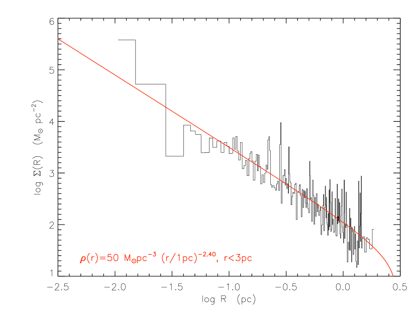
Figure 8.— Measured mass surface density profile of the ONC, adopting the sample of sources with available stellar parameters or X-ray membership (black line). The red line shows the best fit of a truncated 3D power law profile.

Following the work of Hillenbrand & Hartmann (1998), we study the radial density profile of the stellar population in ONC. For simplicity here we neglect the ellipticity of the cluster and derive an average radial profile, adopting circular symmetry in the plane of sky. We consider all the stellar catalogs described in §2; as anticipated, these have been restricted to a square area with a size of 0.4^∘ (2.9 pc) centered on our bona-fide ONC center of mass (§1), where we have full coverage for the optical, near infrared and Spitzer catalogs. The maximum distance from the center to the corners of this area is thus 0.28^∘ or $\sim$2 pc. We divided the samples in radial annuli, each containing 10 stars, up to the maximum distance from the center, and measured the projected stellar mass density summing the stellar masses in each annulus and dividing the result by the area of each annulus. As in §3.4, stars with no available mass estimate had been assigned a mass of 0.5 $M_{\odot}$. The results for the outer annuli, which are in part outside our square field of view, have been corrected to account for this incompleteness.

The mass surface density profile of the ONC has been computed for different combinations of the stellar samples. In particular, we considered the full photometric samples (optical, near infrared and Spitzer), the sub-samples of sources with optically derived parameters, the youth tracers (IR excess, X-ray emission), and several combinations of these selection criteria. An example of these surface stellar density profiles is shown in Figure 8, for the sample of sources with either optically derived parameters or X-ray membership.

Unlike in Hillenbrand & Hartmann (1998), our mass surface density profiles $\Sigma(R)$ tend not show a flattening in the core regions, but appear to follow roughly a straight line in logarithmic axes in the entire radial range. Thus, instead of adopting King models, we assume that the 3D stellar density $\rho(r)$ follows a power-law profile up to a maximum radius $r_{\rm max}$ which sets the boundary of the cluster:

$$\rho(r)=\begin{cases}\rho_{0}\ \bigg{(}\displaystyle\frac{r}{\rm 1pc}\bigg{)}^{-\alpha}&\text{if }r\leq r_{\rm max}\\ 0&\text{if }r>r_{\rm max}\end{cases}$$

We assume $r_{\rm max}=3$ pc, and varying $\alpha$ we project the 3D $\rho(r)$ in 2D for $\Sigma(R)$; these latter are then fit to the data using a $\chi^{2}$ minimization, thus determining the best fit $\alpha$ and $\rho_{0}$.

Table 2ONC population density profile parameters

Sample	$\rho_{0}$	$\alpha$	$N_{*}$ $(<2$ pc)	$M_{*}$ ($<2$ pc)
	$(M_{\odot}{\rm pc}^{-3})$			$(M_{\odot})$
a) all sources	105	2.05	4323	$2676$
b) $JHK$ photometry	95	1.98	4129	$2386$
c) $JHK_{\rm stellar}$	55	2.25	2745	$1539$
d) optical photometry	52	1.90	2969	1285
e) optical parameters	33	2.05	1927	846
string f) young	17	2.24	1009	465
string g) old	17	1.88	939	405
h) optical param + X-ray	50	2.40	2595	1591
i) optical param + X-ray + IR excess	55	2.35	2741	1667
j) optical param + IR excess	46	2.02	2238	1156
k) IR excess	23	2.01	1094	578
l) optical param + X-ray + $JHK_{\rm stellar}$
string$A_{V}<1$ mag	18	1.96	915	452
string$A_{V}<3$ mag	32	2.29	1621	916
string$A_{V}<10$ mag	50	2.26	2733	1421
string$A_{V}<30$ mag	66	2.24	3132	1850
string$A_{V}<100$ mag	66	2.27	3230	1886

Note. — Samples are defined as follows. $a)$: any individual source detected in the optical photometry of Da Rio et al. (2010a), the NIR photometry of Robberto et al. (2010) complemented with 2MASS, Spitzer and X-ray members from Getman et al. (2005b); $b)$: NIR photometry catalog; $c)$: as b) but excluding sources in the CMD zone populated by brown dwarfs and contaminants (see Robberto et al. 2010); $d)$: optical photometry from Da Rio et al. (2010a); $e)$: sample of optically derived stellar parameters from Da Rio et al. (2012); $f)$ and $g)$: sources with available age estimate from the HRD, divided as younger or older than the mean cluster age. $k)$: Spitzer detection showing evidence of IR excess from circumstellar material (Megeath et al., 2012). From $h)$ to $l)$: combination of the above criteria.

Table 2 reports the best-fit density profile parameters, as well as the extrapolated number of sources and total stellar mass within 2 pc from the center. Overall, the power law exponent $\alpha$ is found to be close to that of single isothermal sphere ($\alpha_{\rm SIS}=2$), and only weakly affected by the criteria for selecting the stellar sample, despite a factor of several difference in the number of stars. The values $\alpha\gtrsim 2.3$ obtained for samples that include the X-ray sources is in part biased towards steeper slopes by the incomplete X-ray coverage at large distances from the center. Conversely, the optical photometric catalog shows a flatter slope than other samples, possibly due to lower completeness in the central regions of the ONC because of the bright nebular background in the vicinity the Trapezium. Similarly, stars with isochronal ages older than the mean cluster age are more likely to be missed in the central regions, as they are fainter than younger sources for the same mass. Lastly, the exponent from the fit to the entire $JHK$ photometry, which include prominent background contamination at substellar luminosities, turns out to be flatter than that obtained restricting to the stellar mass range, where contamination is minimal. This is expected as the contamination from Galactic field sources is not as centrally concentrated as the ONC members. From all these comparisons, we estimate a bona fide value $\alpha\simeq 2.2$ for the ONC population. We emphasize that in principle a power law density profile is unphysical, in that it has infinite density at $r=0$. However, for $\alpha<3$ the mass contribution of the core does not diverge, and for the isothermal case each radial bin in linear units contributes the same amount of mass. Since our measurements find no deviation from a single power law down to $r\sim 10^{-2}$ pc, changing the model to remove the singularity at smaller radii would have no effect on our analysis.

The assessment of the real value of $\rho_{0}$ from the values listed in Table 2 is critical to constrain the actual stellar mass of the ONC, and requires some considerations. First the value $\rho_{0}\simeq 100\>M_{\odot}{\rm pc}^{-3}$ determined for entire sample of unique detections summed from each catalog, as well as the whole $JHK$ sample, is significantly overestimated due to the large contamination at faint luminosities. The normalization value, hence the total mass of the cluster nearly halves when restricting to near infrared sources above the stellar mass threshold of Robberto et al. (2010), below which nearly each source is not a member. Even this sample, however, suffers from some contamination and some incompleteness. For example, within the same field of view and luminosity range ($M\gtrsim 0.2\>M_{\odot}$), $\sim 15\%$ of NIR sources are not X-ray members; this increases to $\sim 25\%$ in the whole stellar luminosity range; this is both due to increasing incompleteness of the X-ray survey, and increasing contamination towards lower luminosities. However, the X-ray sample reaches deeper extinctions than our JHK photometry. Within an aperture of 0.11^∘ from the ONC center, we find 25% of X-ray sources with no counterpart in the $JHK$ stellar sample. Thus, incompleteness and contamination should roughly cancel out, in stellar number, in the stellar luminosity range of the $JHK$ sample. Yet, this sample will be affected by further incompleteness, at faint luminosities under the stellar threshold in the $JH$ CMD, and somewhat in the core of the region, where confusion limits the X-ray sample. This can be noted from Table 2 considering the sample of optically derived parameters (which extends somewhat in the substellar regime), X-rays and IR excess sources: this sample is virtually immune from contamination but likely incomplete, outside the FOV of the X-ray sample, and at low luminosities near the core. Its measured normalization constant $\rho_{0}=55~{}M_{\odot}\>{\rm pc}^{-3}$ is identical to that of the $JHK$ sample at stellar luminosities.

Based on the above data, it is not clear what the degree of residual incompleteness is in these samples that is caused by substellar objects, unresolved binaries, and confusion in the center. With some uncertainty, we thus assume an additional $25\%$ of total stellar mass. Thus we infer that the ONC stellar population is well represented by a density distribution:

$$\rho_{\rm stars}(r)\simeq\ 70~{}M_{\odot}~{}{\rm pc}^{-3}\bigg{(}\frac{r}{1{\rm pc}}\bigg{)}^{-2.2},\ r<3{\rm~{}pc}.$$ (3)

We emphasize that this simple model is intended to be representative of the overall dynamical contribution from stellar mass in the ONC; on smaller scales some degree of substructure, as well as elongation, remain present (see §3). Other studies (e.g., Rivilla et al., 2013; Kuhn et al., 2014) have also analyzed the spatial structure of the ONC population within the inner pc of the region, finding that the stellar distribution is well matched by a superposition of a denser core - basically coincident with the Trapezium - surrounded by a shallower halo.

Last, as we have shown in Section 3, the heavily embedded population, though it accounts for a small fraction of the population, appears slightly offset from the main cluster, following the densest cores in the region and the integral shape filament within the OMC-1. In this study we do not consider this part of the population as a separate population to be removed from the sample, as we infer it will eventually be one with the rest of the system during the upcoming early evolution of the ONC. However, we check if the spatial distribution of the heavily embedded population affects the surface density profiles we have derived. The last rows of Table 2 report the fitted profile parameters for the sample of sources with available $A_{V}$ (either optical spectroscopy, NIR CMD, or X rays), limited below varying upper limits in extinction. Except for the lowest extinctions, which appear slightly less centrally concentrated, most likely since they belong to the very external shell of the system toward our direction, the power law exponent remains largely unaffected by the chosen cut in extinction.

4.2. ISM density

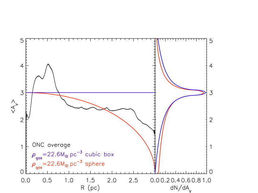
Figure 9.— Average extinction affecting the ONC members as a function of projected radius from the center, obtained from the average ONC members $A_{V}$ map from Scandariato et al. (2011).

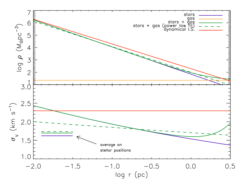
Figure 10.— Top panel: The estimated volume density profile of the ONC due to stars, gas, and total (stars + gas), together with the best power-law fit to the latter as reported in the Legend. The red line represents the density profile of a singular isothermal sphere needed under the assumption of dynamical equilibrium given the observed velocity dispersion in the system (§4.3). Bottom panel: the predicted 1D velocity dispersion, $\sigma_{v}$ as a function of radius for the these models. The horizontal lines on the left indicate the overall cluster $\sigma_{v}$, computed averaging the curves with a weighting proportional to the fractional stellar mass at each radius.

The distribution, density and total mass of the ISM in the ONC is not well constrained. Some of the densest regions of the OMC cloud (the KL region and the OMC-1 South cores) can reach column densities of up to $A_{V}\sim 100$ mag (Bergin et al., 1996; Scandariato et al., 2011; Lombardi et al., 2011), but the total mass estimates of these clumps and cores can be uncertain by at least a factor of two, given uncertainties in temperatures, dust emissivities and gas to dust mass ratios. In addition much of the gas in the region lies somewhat behind the ONC. This is demonstrated by the large difference between the total ISM column densities integrated along the line of sight and the relatively small extinction affecting ONC stellar members which peaks at $A_{V}=1$–$2$ mag and presents a tail extending to $A_{V}\gtrsim 5$–$10$ mag (Hillenbrand, 1997; Da Rio et al., 2010a). As anticipated, only a minor fraction of young stellar members appear highly obscured.

Scandariato et al. (2011) used near-infrared data, together with optical parameters where available, to derive both the total extinction map – from statistics of background stars – as well a map of the average $A_{V}$ affecting the ONC members. We have adopted the latter and computed its mean value as a function of angular distance from the center of the ONC. The result is shown in Figure 9. The mean stellar $A_{V}$ is nearly constant at all distances from the centers, at a value $\langle A_{V}\rangle\simeq 2.5$–$3$ mag. The peak extiction at $R\simeq 0.5$pc is due to the Dark Bay (O’dell, 2001), an obscuring cloud in slight foreground with respect to the ONC population and HII region, located north-east of the Trapezium.

If we assume that the ISM is uniformly distributed also along the line of sight, we can translate this column density of dust into a total volume density of ISM. Since the $A_{V}$ distribution is skewed, this is probably not the case, and the ISM density on average increases moving into the cluster along the line of sight, reaching high values for the few very embedded objects. However, this approximation is fair at the midplane of the system. If we thus assume that the ISM is uniformly distributed in either a cubic box or a sphere around the cluster center with the radius of 3 pc, the same truncation we have assumed in Figure 8 for the stellar distribution, this translates into an optical depth $A_{V}=1~{}{\rm mag\>pc}^{-1}$ along the line of sight. Assuming the dust to gas relation from Vuong et al. (2003) $N_{\rm H}/A_{V}=1.58\times 10^{21}~{}$cm^-2 and solar abundance of He, this corresponds to a constant gas density:

$$\rho_{\rm gas}\simeq 22~{}M_{\odot}~{}{\rm pc}^{-3}.$$ (4)

It could be argue that part of the extinction towards ONC sources may originate from foreground galactic ISM unrelated to the cluster. E.g., O’Dell et al. (2008) finds that the Orion Nebula HII region is obscured by $A_{V}\sim 2$ mag of neutral material. However, the vast majority of such veil remains located within the stellar system, meaning that part of the ONC population is well in front of the HII region. This is confirmed by the fact that spectroscopic measurements of extinctions towards individual ONC members (Hillenbrand, 1997; Da Rio et al., 2010a, 2012) measure $A_{V}$ values as low as $\sim 0$ with no evidence, within the uncertainties, of a positive minimum threshold value. Therefore the foreground extinction from Galactic ISM must be of negligible amount, up to no more than a few tenths of magnitude, negligible compared to the mean ONC extinction shown in Figure 9). Given the relatively large uncertainties already present in our mass estimates for both stars and gas, we thus do not attempt to constrain and remove the small foreground extinction.

Figure 9 also shows, together with the radial trend of the average $A_{V}$, the trend expected assuming this uniform amount of ISM either in a cubic or spherical geometry; in both cases the simple model is fairly adequate to reproduce the data.

The $A_{V}$ map from Scandariato et al. (2011) was derived from NIR data, thus lacking potentially heavily embedded sources that could, although they are a small fraction of the population, shift the mean stellar $A_{V}$ to higher values. We have thus also considered the extinctions derived from $\log N_{\rm H}$ from the COUP X-ray sample. Indeed, the X-ray mean $A_{V}$ is $\sim 15$ mag; this value however is strongly biased by the asymmetry of the distribution, with a few sources with derived values exceeding 100 mag, and large relative errors in the measurements. The median $A_{V}$ is 3.8 mag, in line with the mean from Scandariato et al. (2011). Also, the errors in $A_{V}$ from the X-ray analysis correlate with $A_{V}$, and the values of $N_{\rm H}$ appear nearly symmetric around a mean value of $10^{21.7}$ cm^-2, which corresponds to $A_{V}\simeq 3$. Thus we conclude that our estimate for the value $\rho_{\rm gas}\simeq 22\>M_{\odot}\>{\rm pc}^{-3}$ adequately represents the present average ISM content within the ONC.

The above ISM density, when compared to the stellar mass profile (Equation 3) is quite small: it is smaller than the stellar density for $r<1.37$ pc, radius containing $73\%$ of the stellar mass within 2 pc, or $53\%$ within 3pc, and negligible in the cluster core. If we approximate the contribution of stars and gas to the radial profile with a power law, the results depends on the considered range in radii. Limiting to the range of distances spanned by our stellar density profiles (e.g., Figure 8), the approximate total density follows

$$\rho_{\rm total}\sim 100\bigg{(}\frac{r}{1\>{\rm pc}}\bigg{)}^{-2.07}\>M_{\odot}\>{\rm pc}^{-3}.$$ (5)

We will utilize this as an estimate for the total observed mass, for comparison with the dynamical mass (§4.3). Figure 10 summarises the contribution to the density profile from equations 3 and 4, and the approximation to the total of equation 5.

4.3. Dynamical Equilibrium

It has been pointed out in several works (e.g., Hillenbrand & Hartmann, 1998; Scally et al., 2005) that the ONC may not be in dynamical equilibrium, as the dynamical mass determined from the kinematic properties of the cluster is twice or more the stellar mass. Here we follow up on these findings based on our updated estimates of stellar and gas content in the ONC (§4.1 & 4.2).

Proper motions surveys in the ONC date back to the work of (Jones & Walker, 1988); they measured a 1 dimensional velocity dispersion $\sigma_{v}\simeq 2.3$ km s^-1. Radial velocity surveys Sicilia-Aguilar et al. (2005); Fűrész et al. (2008); Tobin et al. (2009) derived a nearly identical velocity dispersion within the ONC region, except for evidence for lower velocities ($<1.8$ km s^-1) for bright members, and systematic variations with position at scales larger than that considered in this study, along the north-south filament.

If we consider a singular isothermal profile $\rho(r)=\rho_{0,{\rm SIS}}~{}r^{-2}$, which given the power law exponents 2.2 or 2.07 from Equations 3 and 5 is a fair approximation for the ONC, an average $\sigma_{v}=2.3$ km s^-1, under dynamical equilibrium would imply a normalization constant for the density at $r=1$ pc of

$$\rho_{0,{\rm SIS}}=\frac{\sigma_{v}^{2}}{2\pi G}=37\bigg{(}\frac{\sigma_{v}}{1~{}{\rm km~{}s}^{-1}}\bigg{)}^{2}~{}M_{\odot}~{}{\rm pc}^{-3}\rightarrow 195~{}M_{\odot}~{}{\rm pc}^{-3}.$$ (6)

This is about twice the overall value we have estimated from the contribution of stars and gas in the ONC (Equation 5). Alternatively, if we consider that the best power law fit of the estimated stellar plus gas density (Equation 5) has an exponent close to that of an isothermal sphere, its normalization $\rho_{0}=100~{}M_{\odot}~{}{\rm pc}^{-3}$ would lead to a velocity dispersion $\sigma_{v}\simeq 1.64\>{\rm km\>s^{-1}}$ if in virial equilibrium.

In §5, below, we find evidence for relatively prolonged star formation history and thus gradual build-up of the ONC, in which case one expects a virialized star cluster to be established before gas removal (e.g., Fellhauer et al., 2009). However, subvirial initial conditions for stellar motions are also a possibility as suggested by studies of dense gas cores (Kirk et al., 2007, e.g.,)), with subsequent dynamical evolution investigated by a number of works (e.g., Proszkow & Adams, 2009; Allison et al., 2009; Parker & Meyer, 2012). In this case, the initial density structure would have an even higher normalization than that implied by Equation 6 (but within the context of a static density structure that does not account for cluster expansion or contraction).

We better characterize the radial dependence of the predicted $\sigma_{v}$ from the actual measured density profile of stars alone and with gas from Equations 3, 4 and 5. For simplicity we assume isotropic velocities and thus $\sigma_{v}=v_{\rm rot}/\sqrt{2}$, which would strictly hold for a model in equilibrium, and where $v_{\rm rot}$ is the Keplerian rotational velocity for circular orbits in the potential described by our volume density profile. The result is shown in the bottom panel of Figure 10; we find that given the actual volume density of stars and gas in the ONC, virial equilibrium would require $\sigma_{v}\simeq 1.73$, which is $75\%$ of the measured velocity dispersion. This indicates that the ONC may be slightly super-virial, with a virial ratio (kinetic over potential energy) $q\simeq 0.9$;

In this case, the ONC cannot be in perfect dynamical equilibrium, and should be expanding. This result, however, is affected by some degree of uncertainty, since it relies on our estimate of total stellar and gas mass – which remains a challenging estimate (§4.1) – as well as velocity dispersion measurements from proper motions and/or radial velocity surveys, which in turn are very sensitive to membership estimates, measurement accuracy and binary properties of the ONC members.

A current supervirial state of the ONC would be consistent with general theoretical expectations of dynamical evolution, either quickly or slowly compared to the dynamical time, from an initially virialized state as gas is expelled by feedback during the star cluster formation process. Alternatively, dynamically fast star cluster formation scenarios can be imagined in which the natal, transient gas cloud was always in a supervirial state, e.g., if it was formed or affected by large-scale gas flows (Hartmann et al., 2012; Bonnell et al., 2006).

A supervirial state leading to cluster expansion and dissolution is also consistent with observed populations of young clusters that exhibit high “infant mortality” with most clusters of a given mass not surviving at that mass during their first 10 Myr of evolution, most likely because of their relatively low overall star formation efficiencies from their natal gas clumps (e.g., Lada & Lada 2003).

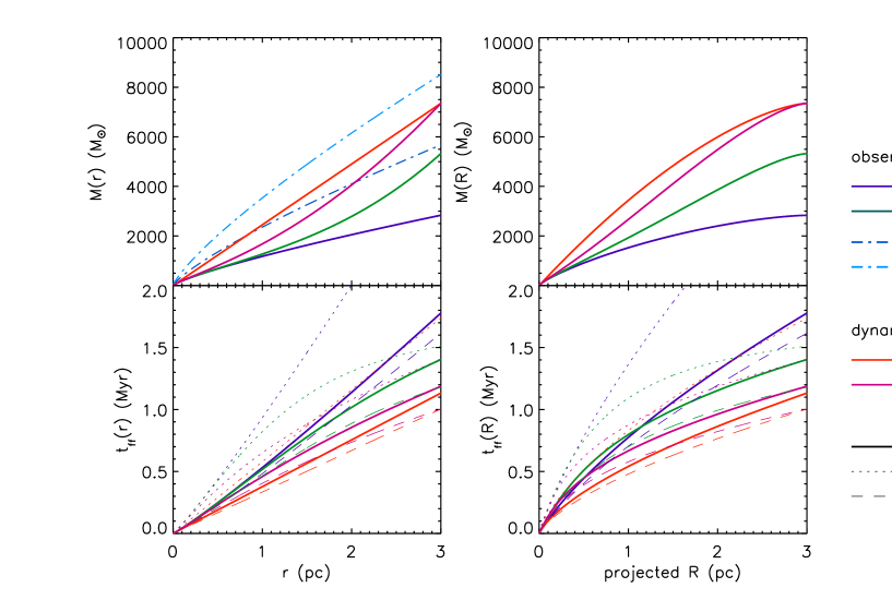
Figure 11.— Cumulative mass (upper panels) and free-fall time (bottom panels) as a function of 3D radius, $r$, (left panels) and projected 2D radius, $R$, (right panels) for four density distributions: only the stellar mass profile ($\rho_{\rm gas}=0$) (purple lines); the stellar plus gas density from Equations 3 and 4 (green); the isothermal profile that matches the observed $\sigma_{v}$ in dynamical equilibrium (red); the sum of the present-day density profile plus a $\rho\propto r^{-1}$ gas profile in order to have a total mass at $r<3$ pc identical to the previous isothermal model (magenta). Solid lines are the exact integration from every distance in the given potential, compared to the approximation $t_{\rm ff}=[3\pi/(32G\rho)]^{1/2}$ assuming the local $\rho$ (dotted line) or the mean $\langle\rho\rangle$ within each radius (dashed line).

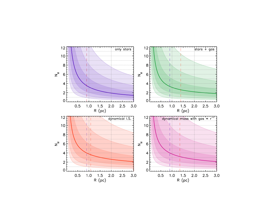
Figure 12.— Radial variation (in projected 2D radius, $R$) of the mean age of the ONC expressed in free-fall times for the four models shown in Figure 11 (thick line). The shaded contours delimit the $1\sigma$, $2\sigma$ and $3\sigma$ widths of the log-normal age spread as constrained in the literature (see text). The vertical dashed black line shows the half-mass radius of the observed stellar density profile, while the vertical dashed red lines the half-mass radius of the particular combination of total mass (gas + stars) for each model.

5. Star Formation Efficiency per Free-Fall Time

A long standing debate in the star formation community concerns the timescales over which a molecular clump sustains star formation, i.e., the duration of star cluster formation. “Fast” scenarios (Elmegreen, 2000; Hartmann et al., 2001; Elmegreen, 2007; Hartmann & Burkert, 2007) predict that star-forming clumps are relatively transient dynamical entities, with star cluster formation extending over just one or a few free-fall or dynamical times. The star formation efficiency per (local) free-fall time, $\epsilon_{\rm ff}$, would then be relatively high, $\gtrsim 0.1$, depending on the overall star formation efficiency that is achieved in the forming the cluster from the clump.

Alternatively, in the “slow” mode the process is sustained in quasi-equilibrium for at least several crossing times (e.g., Tan et al., 2006; Nakamura & Li, 2007), with star formation regulated by turbulence that is maintained by protostellar outflows or by support from relatively strong magnetic fields. In these models, $\epsilon_{\rm ff}$ is relatively low, $\lesssim 0.1$. There is also more time available for continued accretion of gas to the star-forming clump from its surroundings.

The extent of the age spread in the ONC (as well as in other clusters) has been recently constrained by a number of works. The luminosity spread of its PMS stars, if interpreted as a distribution in radii for a given mass from a true age spread leads to a large apparent width ($\sigma_{\log t}=0.4$ dex, Hillenbrand 1997; Da Rio et al. 2010a) around a (model dependent) mean age of $\sim 2.5$ Myr. Observational uncertainties, variability and unresolved binarity cause this age spread to be overestimated, however. Reggiani et al. (2011) showed that these have a small effect on the overall luminosity broadening. Jeffries et al. (2011) on the other hand posed an upper limit to the real $\sigma_{\log t}$ of 0.2 dex, from the lack of correlation between the abundance of circumstellar disks around members and isochronal ages, suggesting that the apparent luminosity spread is in large part – if not all – due to protostellar accretion induced changes in the stellar structure evolution (Baraffe et al., 2009, 2012). However, Hosokawa et al. (2011) found that reasonable levels of episodic accretion were insufficient to explain the observed luminosity spread, suggesting significant intrinsic age spreads are present. Lastly, Da Rio et al. (2014) excluded a very short age spread, from an analysis of the bias in the inferred temporal decay of mass accretion rates induced by uncertain ages of PMS stars, suggesting as a bona fide compromise of all these independent constraints that there is a real age spread $\sigma_{\log t}=0.2$ dex around a mean age $t=2.5$ Myr, corresponding to 95% of the ONC population with ages between 1 and 6.3 Myr assuming a Gaussian distribution in $\log t$. If instead a uniform distribution in $\log t$ is assumed, this 95% of the stars lie in the interval between 1.1 and 5.5 Myr, and for a gaussian distribution in linear age between 0.7 and 4.7 Myr. We stress that given the amplitude of the apparent age spread compared to the real one, the actual shape of the age distribution is largely unknown; this is also particularly true at very young ages, where the age of individual sources is largely uncertain. Hereafter we will assume a lognormal distribution.

Here we utilize our constrained estimate of the stellar and gas content of the ONC to translate the age and age distribution of the ONC in terms of free-fall timescales. We consider different models for the mass content of the region: first, the present-day estimates, separately for the radial distribution of mass volume density of stars alone (Equation 3) and the sum of stars and gas (Equation 4). Second, assuming that the supervirial state of the ONC we have found in §4.3 is due to recent gas expulsion, we consider two simple assumptions for the total mass profile before this event: the singular isothermal sphere that reproduces the observed velocity dispersion (Equation 6) and a model obtained adding to the measured present-day stellar density profile a gas profile $\rho_{\rm gas}\propto r^{-1}$ normalized so that the total mass contained within $r<3$ pc coincides with that of the latter isothermal sphere.

Figure 11 shows the radial dependence of both the cumulative mass, and the free-fall time $t_{\rm ff}$ for each model. The solid lines for $t_{\rm ff}$ represent the exact $t_{\rm ff}$ calculated by numerical integration of the motion of a test particle from rest within the modeled potential. For comparison, we also show the resulting $t_{\rm ff}$ derived adopting the common approximation valid for a uniform sphere, $t_{\rm ff}=[3\pi/(32G\rho)]^{1/2}$, where we assume for the volume density $\rho$ either the local one at any given $r$ (dotted lines in Figure 11) or the average density within the sphere of radius $r$ (dashed line). The first approximation leads to an overestimation of $t_{\rm ff}$, since in reality the density increases moving towards the center. On the other hand the second approximation leads to results closer to the exact solution, although in this case $t_{\rm ff}$ are slightly underestimated. In Figure 11 we also show the mass profile obtained by simply multiplying the stellar mass by two and three. This shows that the two models that reproduce the dynamical state in equilibrium are also compatible with a simple assumptions that the ONC initially had a similar a similar density profiles as the present-day stellar distribution, and stars have formed with an efficiency between $\sim 30$ and 50%. In this case most of the remaining gas has been expelled by the system during the star cluster formation process.

Using these four models, Figure 12 shows the mean age of the ONC, together with its age spreads in units of 1, 2 and 3$\sigma$ from the mean age, expressed in terms of the number of free-fall times, $N_{\rm ff}$, in the past at different distances from the cluster center. To this end we have assumed, as mentioned, a log-normal age distribution with a width of 0.2 dex around a mean age of 2.5 Myr. Of course the system becomes increasingly dynamically older towards the core, even under the assumption of constant average age and age spread, due to the shorter free fall time at higher densities.

Figure 12 also highlights that the age distribution of the ONC spans on average several $t_{\rm ff}$ depending on the model. This is clarified in Figure 13, left panel; this shows, again as a function of projected radius from the center, the number $N_{\rm ff,90}$ of free fall times needed form $90\%$ of the stellar population, in a symmetric interval with respect to the mean cluster age, for the four models. When considering the present-day mass distribution, either from stars alone or from stars and present gas (blue and green) at the half-mass radius, 90% of the stellar population has been forming within 5 to 6 free-fall times. Including the contribution to the missing mass needed for the ONC to be in dynamical equilibrium, (red and magenta) increases the number of $t_{\rm ff}$ from 6 to 8 at the same radii, due to the shorter $t_{\rm ff}$ for these models. In any case, we find these results to be compatible with a slow star formation scenario.

If star cluster formation takes place over a relatively extended period of time, a natural question to ask is whether the characteristics of star formation, such as the initial mass function, change systematically during this evolution. Or even more simply, do massive stars tend to form preferentially near the beginning or end of star cluster formation? If feedback from massive stars is the primary agent terminating star cluster formation, then one may expect they will tend to form near the end of the process. In the ONC, Da Rio et al. (2012) did not find any evidence for a stellar mass versus age correlation, although such analyses are subject to inherent systematic uncertainties arising from pre-main sequence stellar evolutionary models. On the other hand, Getman et al. (2014) found the ONC core, where most of the massive stars are located, to be younger than the outskirts. While massive stars are still forming today in the ONC, such as “source I” in the KL region (see Tan et al. 2014 for a review), (Hoogerwerf et al., 2001) have claimed that the four massive ($\sim 20\>M_{\odot}$) stars $\mu$ Col, AE Aur and the $\iota$ Ori binary formed in the ONC and were dynamically ejected about 2.5 Myr ago. This timescale is compatible with the age spread we have adopted from the analysis of Da Rio et al. (2012) and would indicate that massive star formation, at least in the case of the ONC, has occurred throughout the star cluster formation process. It also suggests that the destructive feedback from massive star formation can be mitigated by dynamical (self-)ejection of the massive stars—a process likely enhanced by their migration to the cluster center, as perhaps exemplified today by the case of $\theta^{1}$C and its recent interaction with BN (Tan, 2004; Chatterjee & Tan, 2012).

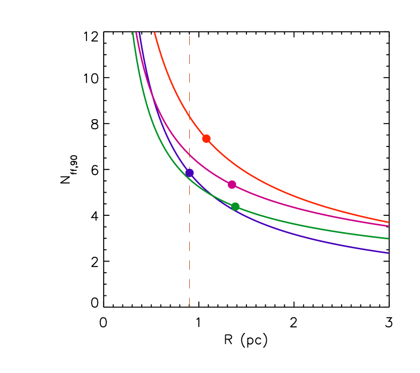
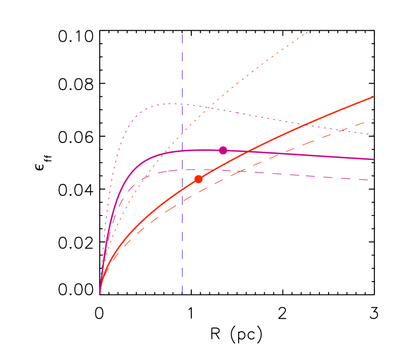
Figure 13.— Left panel: Number of free-fall times needed for the formation of 90% of the stellar population in the ONC, as a function of the projected 2D radius, $R$, from the center, for the four models shown in Figure 11. The filled circles denote the half-mass radius each model, and the dashed vertical line the present-day half mass radius of the stellar density profile. Right panel: Star formation efficiency per $t_{\rm ff}$ as a function a radius, for the two models representing possible initial conditions before gas removal.

The right panel of Figure 13 shows the star formation efficiency per free-fall time, $\epsilon_{\rm ff}$. This is simply estimated as $\epsilon_{\rm ff}=0.9\epsilon_{*}t_{\rm ff}/t_{\rm form,90}=0.9\epsilon_{*}/N_{\rm ff,90}$, where $\epsilon_{*}$ is the fraction of total mass converted into stars. Since in Figure 13 we adopt the projected 2D radius, here we assume $\epsilon_{*}=\Sigma_{*}/\Sigma_{\rm tot}$ instead of $\rho_{*}/\rho_{\rm tot}$, as well as the projected $t_{\rm ff}$ as shown in the bottom-right panel of Figure 11. As in the previous figures, the red and magenta lines are for the two models we adopt for the mass content before gas removal, respectively the isothermal sphere reproducing the observed $\sigma_{v}$ and the stellar profile with gas $\sim r^{-1}$. The value of $\epsilon_{\rm ff}$ decreases towards the core, as a consequence of the smaller $t_{\rm ff}$ compared to the age spread which we assumed radially constant (consistent with the results of Da Rio et al. 2012).

On the other hand, the slow decrease in $\epsilon_{\rm ff}$ at larger radii for the model with a shallower gas profile is due to the radial decrease of $\epsilon_{*}$ since the stellar profile falls more steeply than the gas in this model. The circles in this figure denote the value at the half-mass radius, where we find $\epsilon_{\rm ff}\simeq 0.05$. For comparison, in Figure 13 we also show the same quantity derived from the two approximations of $t_{\rm ff}$ as computed from the local density at each radius, or the mean density enclosed within each radius, as in Figure 11.

Our derived values of $\epsilon_{\rm ff}$ are very similar to the value adopted in the study of Krumholz & Tan (2007). It is comparable to the values seen in the simulations of Nakamura & Li (2007), in which star formation activity is regulated by protostellar outflow driven turbulence.

6. Conclusions

In this work we have reanalyzed the structural and dynamical properties of the ONC. We based our analysis on a collection of stellar catalogs, membership estimates and stellar properties from the latest studies: optically derived stellar parameters, near-infrared photometry, Spitzer photometry and X-ray data. We have used previous studies to assess the level of contamination from the Galactic field in order to constrain the actual stellar population of the system. Last, we use stellar $A_{V}$ properties to estimate the ISM density within the cluster as an additional component adding to the gravitational potential. Here we briefly summarize our findings.

1. We determine the center of mass of the ONC, from a subsample of sources of known membership. The center is located within the Trapezium region, and its position is only weakly sensitive on the assumptions for sources without available stellar parameters. We also note that the center roughly coincides with the location of the point where, according to Chatterjee & Tan (2012), the dynamical ejection of the BN object from $\theta^{1}$C took place. $\theta^{1}$C, being the most massive star in the cluster, is expected to migrate to this location via dynamical interactions with other cluster stars, which thus places a joint constraint on the age of the star and the distance of its formation site from the cluster center.

2. We analyze the degree of angular substructure of the spatial distribution of stars via the angular dispersion parameter, $\delta_{\rm ADP,N}$, including its radial dependence. A random azimuthal distribution leads to $\delta_{\rm ADP,N}\simeq 1$, whereas a degree of additional intrinsic substructure, perhaps imparted from initial turbulence in the star-forming gas, increases its value. The measured $\delta_{\rm ADP,N}$ in the ONC lies between that measured in Globular clusters – as dynamically old stellar systems with no azimuthal substructure – and Taurus, chosen as an example of a very young, dynamically unevolved, clumpy stellar system. The dispersion is found to be lower in the core of the ONC compared to the outskirts, indicating of higher dynamical processing that has erased any initial substructure. However, we also find that the elongation of the system along the north-south direction, higher at increasing distances from the center, is the major contributor to the measured increase of $\delta_{\rm ADP,N}$ with radius, if ellipticity is not accounted for. We test the dependence of the radial trend of the dispersion on the selection of stellar samples, finding no significant variations when different combinations of the stellar catalogs are used.

3. We derive the stellar mass surface density and volume density profiles of the ONC, for different combinations of the catalogs affected by varying degrees of incompleteness and contamination. This allows us to accurately extrapolate the bona fide profile of the ONC members, which is well reproduced by a power-law profile (Equation 3). We use measured stellar $A_{V}$ to derive the average gas density within the cluster, which appears to be nearly constant at $\rho_{\rm gas}\sim 22\>M_{\odot}\>{\rm pc}^{-3}$, i.e., relatively small compared to the stellar density except at large distances from the center.

4. We compare the total estimated mass density profile of the ONC with literature measurements of the velocity dispersion $\sigma_{v}$ in the region, confirming previous claims that the cluster is slightly supervirial, indicative that the ONC should be expanding. We expect that this supervirial state has most likely been caused by relatively recent gas expulsion, given that the duration of star formation appears to have been relatively long compared to the free-fall or dynamical time (below).

5. We derive the radial dependence of free-fall time, $t_{\rm ff}$, assuming either the present-day measured mass density and different simple models for that required by dynamical equilibrium, as descriptive of possible configurations before gas disperal. We compare $t_{\rm ff}$ with recent constraints on the age and intrinsic age spread in the ONC: the cluster appears to be at least several $t_{\rm ff}$ old, and $90\%$ of the population has been forming over 5 to 8 $t_{\rm ff}$ depending on the assumptions, consistent with slow star formation scenarios. From these results we infer a star formation efficiency per free-fall time for the cluster-forming gas of $\epsilon_{\rm ff}\simeq 0.05$.

References

- Allison et al. (2010) Allison, R. J., Goodwin, S. P., Parker, R. J., Portegies Zwart, S. F., & de Grijs, R. 2010, MNRAS, 407, 1098
- Allison et al. (2009) Allison, R. J., Goodwin, S. P., Parker, R. J., et al. 2009, ApJ, 700, L99
- Anderson et al. (2008) Anderson, J., Sarajedini, A., Bedin, L. R., et al. 2008, AJ, 135, 2055
- Baraffe et al. (2012) Baraffe, I., Vorobyov, E., & Chabrier, G. 2012, ApJ, 756, 118
- Baraffe et al. (2009) Baraffe, I., Chabrier, G., & Gallardo, J. 2009, ApJ, 702, L27
- Bergin et al. (1996) Bergin, E. A., Snell, R. L., & Goldsmith, P. F. 1996, ApJ, 460, 343
- Bertoldi & McKee (1992) Bertoldi, F., & McKee, C. F. 1992, ApJ, 395, 140
- Bonnell et al. (2006) Bonnell, I. A., Dobbs, C. L., Robitaille, T. P., & Pringle, J. E. 2006, MNRAS, 365, 37
- Cartwright & Whitworth (2004) Cartwright, A., & Whitworth, A. P. 2004, MNRAS, 348, 589
- Chatterjee & Tan (2012) Chatterjee, S., & Tan, J. C. 2012, ApJ, 754, 152
- Da Rio et al. (2014) Da Rio, N., Jeffries, R. D., Manara, C. F., & Robberto, M. 2014, MNRAS, 439, 3308
- Da Rio et al. (2012) Da Rio, N., Robberto, M., Hillenbrand, L. A., Henning, T., & Stassun, K. G. 2012, ApJ, 748, 14
- Da Rio et al. (2010a) Da Rio, N., Robberto, M., Soderblom, D. R., et al. 2010, ApJ, 722, 1092
- Da Rio et al. (2010b) Da Rio, N., Gouliermis, D. A., & Gennaro, M. 2010, ApJ, 723, 166
- Elmegreen (2007) Elmegreen, B. G. 2007, ApJ, 668, 1064
- Elmegreen (2000) Elmegreen, B. G. 2000, ApJ, 530, 277
- Feigelson et al. (2005) Feigelson, E. D., Getman, K., Townsley, L., et al. 2005, ApJS, 160, 379
- Fűrész et al. (2008) Fűrész, G., Hartmann, L. W., Megeath, S. T., Szentgyorgyi, A. H., & Hamden, E. T. 2008, ApJ, 676, 1109
- Fellhauer et al. (2009) Fellhauer, M., Wilkinson, M. I., & Kroupa, P. 2009, MNRAS, 397, 954
- Getman et al. (2014) Getman, K. V., Feigelson, E. D., & Kuhn, M. A. 2014, ApJ, 787, 109
- Getman et al. (2005a) Getman, K. V., Flaccomio, E., Broos, P. S., et al. 2005, ApJS, 160, 319
- Getman et al. (2005b) Getman, K. V., Feigelson, E. D., Grosso, N., et al. 2005, ApJS, 160, 353
- Grellmann et al. (2013) Grellmann, R., Preibisch, T., Ratzka, T., et al. 2013, A&A, 550, A82
- Grosso et al. (2005) Grosso, N., Feigelson, E. D., Getman, K. V., et al. 2005, ApJS, 160, 530
- Gutermuth et al. (2009) Gutermuth, R. A., Megeath, S. T., Myers, P. C., et al. 2009, ApJS, 184, 18
- Gutermuth et al. (2005) Gutermuth, R. A., Megeath, S. T., Pipher, J. L., et al. 2005, ApJ, 632, 397
- Hartmann et al. (2012) Hartmann, L., Ballesteros-Paredes, J., & Heitsch, F. 2012, MNRAS, 420, 1457
- Hartmann & Burkert (2007) Hartmann, L., & Burkert, A. 2007, ApJ, 654, 988
- Hartmann et al. (2001) Hartmann, L., Ballesteros-Paredes, J., & Bergin, E. A. 2001, ApJ, 562, 852
- Hillenbrand et al. (2013) Hillenbrand, L. A., Hoffer, A. S., & Herczeg, G. J. 2013, AJ, 146, 85
- Hillenbrand & Hartmann (1998) Hillenbrand, L. A., & Hartmann, L. W. 1998, ApJ, 492, 540
- Hillenbrand (1997) Hillenbrand, L. A. 1997, AJ, 113, 1733
- Hoogerwerf et al. (2001) Hoogerwerf, R., de Bruijne, J. H. J., & de Zeeuw, P. T. 2001, A&A, 365, 49
- Hosokawa et al. (2011) Hosokawa, T., Offner, S. S. R., & Krumholz, M. R. 2011, ApJ, 738, 140
- Huff & Stahler (2007) Huff, E. M., & Stahler, S. W. 2007, ApJ, 666, 281
- Jeffries et al. (2011) Jeffries, R. D., Littlefair, S. P., Naylor, T., & Mayne, N. J. 2011, MNRAS, 418, 1948
- Johnstone & Bally (1999) Johnstone, D., & Bally, J. 1999, ApJ, 510, L49
- Jones & Walker (1988) Jones, B. F., & Walker, M. F. 1988, AJ, 95, 1755
- Kenyon et al. (2008) Kenyon, S. J., Gómez, M., & Whitney, B. A. 2008, Handbook of Star Forming Regions, Volume I, 405
- Kirk et al. (2007) Kirk, H., Johnstone, D., & Tafalla, M. 2007, ApJ, 668, 1042
- Kroupa (2001) Kroupa, P. 2001, MNRAS, 322, 231
- Kroupa et al. (2001) Kroupa, P., Aarseth, S., & Hurley, J. 2001, MNRAS, 321, 699
- Krumholz & McKee (2005) Krumholz, M. R., & McKee, C. F. 2005, ApJ, 630, 250
- Kuhn et al. (2014) Kuhn, M. A., Feigelson, E. D., Getman, K. V., et al. 2014, ApJ, 787, 107
- Lada & Lada (2003) Lada, C. J., & Lada, E. A. 2003, ARA&A, 41, 57
- Lombardi et al. (2011) Lombardi, M., Alves, J., & Lada, C. J. 2011, A&A, 535, A16
- Megeath et al. (2012) Megeath, S. T., Gutermuth, R., Muzerolle, J., et al. 2012, AJ, 144, 192
- Menten et al. (2007) Menten, K. M., Reid, M. J., Forbrich, J., et al. 2007, A&A, 474, 515
- Muench et al. (2008) Muench, A., Getman, K., Hillenbrand, L., & Preibisch, T. 2008, Handbook of Star Forming Regions, Volume I, 483
- Nakamura & Li (2014) Nakamura, F., & Li, Z.-Y. 2014, ApJ, 783, 115
- Nakamura & Li (2007) Nakamura, F., & Li, Z.-Y. 2007, ApJ, 662, 395
- O’Dell et al. (2008) O’Dell, C. R., Muench, A., Smith, N., & Zapata, L. 2008, Handbook of Star Forming Regions, Volume I, 544
- O’dell (2001) O’dell, C. R. 2001, ARA&A, 39, 99
- Padoan & Nordlund (2011) Padoan, P., & Nordlund, Å. 2011, ApJ, 730, 40
- Parker et al. (2014) Parker, R. J., Wright, N. J., Goodwin, S. P., & Meyer, M. R. 2014, MNRAS, 438, 620
- Parker & Meyer (2012) Parker, R. J., & Meyer, M. R. 2012, MNRAS, 427, 637
- Proszkow & Adams (2009) Proszkow, E.-M., & Adams, F. C. 2009, ApJS, 185, 486
- Reggiani et al. (2011) Reggiani, M., Robberto, M., Da Rio, N., et al. 2011, A&A, 534, A83
- Rivilla et al. (2013) Rivilla, V. M., Martín-Pintado, J., Jiménez-Serra, I., & Rodríguez-Franco, A. 2013, A&A, 554, A48
- Robberto et al. (2010) Robberto, M., Soderblom, D. R., Scandariato, G., et al. 2010, AJ, 139, 950
- Sarajedini et al. (2007) Sarajedini, A., Bedin, L. R., Chaboyer, B., et al. 2007, AJ, 133, 1658
- Scally et al. (2005) Scally, A., Clarke, C., & McCaughrean, M. J. 2005, MNRAS, 358, 742
- Scandariato et al. (2011) Scandariato, G., Robberto, M., Pagano, I., & Hillenbrand, L. A. 2011, A&A, 533, A38
- Sicilia-Aguilar et al. (2005) Sicilia-Aguilar, A., Hartmann, L. W., Szentgyorgyi, A. H., et al. 2005, AJ, 129, 363
- Siess et al. (2000) Siess, L., Dufour, E., & Forestini, M. 2000, A&A, 358, 593
- Skrutskie et al. (2006) Skrutskie, M. F., Cutri, R. M., Stiening, R., et al. 2006, AJ, 131, 1163
- Tan et al. (2014) Tan, J. C., Beltran, M. T., Caselli, P., et al. 2014, arXiv:1402.0919
- Tan et al. (2006) Tan, J. C., Krumholz, M. R., & McKee, C. F. 2006, ApJ, 641, L121
- Tan (2004) Tan, J. C. 2004, ApJ, 607, L47
- Tobin et al. (2009) Tobin, J. J., Hartmann, L., Furesz, G., Mateo, M., & Megeath, S. T. 2009, ApJ, 697, 1103
- Vuong et al. (2003) Vuong, M. H., Montmerle, T., Grosso, N., et al. 2003, A&A, 408, 581