Hybrid basis scheme for computing electrostatic fields exterior to close-to-touching discs

Abstract.

This paper presents a simple and effective new numerical scheme for the computation of electrostatic fields exterior to a collection of close-to-touching discs. The method is presented in detail for the two-cylinder case. The key idea is to represent the required complex potential using a hybrid set of basis functions comprising the usual Fourier-Laurent expansion about each circle centre complemented by a subsidiary expansion in a variable associated with conformal mapping of the physical domain to a concentric annulus domain. We also rigorously prove that there is a representation of the solution in the hybrid basis with faster decay rate of coefficients than is obtained by using a non-hybrid basis, thereby providing a rationalization for the success of the method. The numerical scheme is easy to implement and adaptable to the case of multiple close-to-touching cylinders.

1. Introduction

This paper is concerned with a classical problem of great importance in the manufacture of composite materials (see [19] and references therein), as well as in many other applications. It is the determination of the electrical transport properties in two-dimensional media containing a set of embedded inclusions which may be close-to-touching. It is assumed that there is a uniform background field. Lord Rayleigh [22] was one of the first to consider such issues in the context of a regular periodic array of circular inclusions. In this paper we focus on the two-dimensional case, and in ways of calculating the field exterior to the inclusions.

This problem becomes very singular as the inclusions become close-to-touching and this circumstance presents formidable computational problems that have been the subject of much research. In cases there the geometry is sufficiently simple, asymptotic methods can be used to get quantitative insight into this case [16] [17] [18]. The most successful numerical schemes in two-dimensions are integral equation methods. These, nevertheless, also encounter difficulties when the inclusions (or discs) are close-to-touching. Greengard & Moura [13] employed fast multipole-accelerated integral equation methods whose cost grows linearly in the number of unknowns. Since their method does not make any special provision for the singular nature of the problem as the discs get close together, these methods quickly become expensive. Helsing [14] [15] has developed fast multipole-accelerated iterative schemes for inclusions of arbitrary shape. More recently, focussing on the case of arrays of close-to-touching discs, Cheng & Greengard [4] (see also [5]) have presented a method which marries ideas from the “method of images” to various integral equation techniques. Their scheme relies on including multipole expansions, of various orders, about successive generations of reflections (or “images”) of the centres of the discs. These additional reflected terms allow even very singular cases to be resolved to essentially arbitrary accuracy. While the number of multipole expansions involved can become very large, the actual number of unknowns associated with each inclusion is kept small by making use of known reflection operators which allow the coefficients of the expansions about the next-generation images to be inferred analytically from the parent coefficients.

The aim of this paper is to present an apparently new numerical scheme to address the challenge of close-to-touching inclusions. A key advantage of the method is that it is conceptually simple and very easy to implement. The central idea is to make use of a strategically chosen over-complete basis set which we refer to as a “hybrid basis”. The two cylinder problem is studied in detail. In §6 we prove, for the two cylinder problem, that there exists a representation of the solution in terms of a hybrid basis having faster decay rate properties than that obtained through a more traditional non-hybrid method. This provides a rationalization of the empirical observation of superior performance when the so-called “hybrid basis scheme”, to be explained in the next two sections, is used.

2. Problem formulation

Suppose we wish to solve the problem for the electrostatic field exterior to $M$ circular discs, in an $(x,y)$-plane, with the field strength in the far-field tends to the value $E$ at an angle $\chi$ to the $x$-axis. We will repose the problem using a complex variable formulation. The problem is mathematically equivalent to finding the function $w(z)$, analytic and single-valued outside a collection of circular discs, with

(1) $$w(z)\sim E_{0}z+{\mathcal{O}}(1),~{}~{}~{}{\rm as}~{}~{}z\to\infty,$$

where $E_{0}=Ee^{-{\rm i}\chi}\in\mathbb{C}$ and

(2) $${\rm Re}[w(z)]=\biggl{\{}\begin{array}[]{ll}0,&{\rm on~{}}C_{1},\\ \gamma_{j},&{\rm on}~{}C_{j},~{}~{}j=2,3,...,M.\end{array}$$

An identical problem arises in ideal fluid dynamics [3] [6]; it is the problem of finding the uniform flow past a collection of discs where the far-field flow has speed $U$ and angle $\chi$ to the positive real axis. This reduces to finding the function $w(z)$, analytic and single-valued outside a collection of circular discs, with

(3) $$w(z)\sim U_{0}z+{\mathcal{O}}(1),~{}~{}~{}{\rm as}~{}~{}z\to\infty,$$

where $U_{0}=Ue^{-{\rm i}\chi}\in\mathbb{C}$ and

(4) $${\rm Im}[w(z)]=\biggl{\{}\begin{array}[]{ll}0,&{\rm on~{}}C_{1},\\ \gamma_{j},&{\rm on}~{}C_{j},~{}~{}j=2,3,...,M.\end{array}$$

In either problem, the set $\{\gamma_{j}|j=2,...,M\}$ is determined as part of the solution. In what follows, we consider the two physical problems just stated as essentially the same; indeed, they are the same once the identification $w\mapsto{\rm i}w$ is made. We will solve the problem of uniform flow past the discs since convenient analytical solutions to this problem are known (see, for example, Crowdy [6]) and these will be used for bench-marking purposes.

3. Three numerical methods

To illustrate the ideas behind the new method, it is expedient to consider three different numerical schemes for the computation of $w(z)$. These will be referred to as the $z$-scheme, the $\zeta$-scheme and the hybrid scheme. It is the third hybrid scheme which constitutes the new contribution of this paper.

3.1. Fourier-Laurent method (the “$z$ scheme”)

The first scheme, which will be referred to as the “$z$ scheme”, is a standard scheme commonly used in the numerical computation of fields in multiply connected domains. Prosnak [21], for example, makes liberal use of it in the computation of fluid flows in multiply connected geometries.

We describe this method in the context of a two cylinder example. Consider two circular discs, each of radius $s$, centred at $\pm d$ where $d>s$. There is no loss in generality in setting $d=1$ and $|U_{0}|=1$ since all length and time scales can be non-dimensionalized with respect to $d$ and $d/|U_{0}|$ respectively.

A natural approach is to write the following Fourier-Laurent expansion about the centres of the discs:

(5) $$w(z)=U_{0}z+a_{0}+\sum_{k=1}^{\infty}{a_{k}s^{k}\over(z-d)^{k}}+\sum_{k=1}^{\infty}{b_{k}s^{k}\over(z+d)^{k}},$$

where the coefficients $a_{0},\{a_{k},b_{k}|k=1,2,...\}$ are to be determined and the first term clearly enforces the far-field condition. The representation (5) can be substituted into the boundary conditions (4) and evaluated at a set of collocation points which are most naturally chosen to be a set of equally spaced points around the boundary circles. The number of collocation points must be taken to be at least as large as the number of unknown coefficients retained in the truncation. Since the boundary conditions are linear in the unknown coefficients, the latter can be found by a straightforward least-squares solution of the over-determined system.

3.2. Conformal mapping method (the “$\zeta$ scheme”)

A second numerical scheme makes use of a conformal mapping. Consider the conformal mapping from an annulus $\rho<|\zeta|<1$ to the unbounded region exterior to the two discs in the $z$-plane. It is a simple Möbius map given by

(6) $$z(\zeta)=A\left({\zeta-\sqrt{\rho}\over\zeta+\sqrt{\rho}}\right),$$

where

(7) $$\rho={1-(1-(s/d)^{2})^{1/2}\over 1+(1-(s/d)^{2})^{1/2}}$$

and

(8) $$A=d\left({1-\rho\over 1+\rho}\right)=\sqrt{d^{2}-s^{2}}.$$

(There is an abuse of notation here – and throughout – in that $z$ is used both as a coordinate point and as a conformal mapping function.) The point $\zeta=-\sqrt{\rho}$ has been chosen to map to infinity in the $z$-plane. The inverse function to (6) is

(9) $$\zeta(z)=\sqrt{\rho}\left({A+z\over A-z}\right).$$

In this second method, referred to as the “$\zeta$ scheme”, we use the modified representation of $w(z)$ given by

(10) $$w(z)=U_{0}z+C+\sum_{k=1}^{\infty}c_{k}[\zeta(z)]^{k}+\sum_{k=1}^{\infty}{d_{k}\rho^{k}\over[\zeta(z)]^{k}},$$

where the coefficients $C,\{a_{k},b_{k},c_{k},d_{k}|k=1,2,...\}$ are now to be determined. The terms

(11) $$\sum_{k=1}^{\infty}c_{k}[\zeta(z)]^{k}+\sum_{k=1}^{\infty}{d_{k}\rho^{k}\over[\zeta(z)]^{k}}$$

can be recognized as a Laurent series capable of representing any function that is analytic and single-valued in the annulus $\rho<|\zeta|<1$ and hence, under the conformal mapping, in the region exterior to the two discs. As before, the easiest strategy to find the unknown coefficients is to solve an over-determined system by a least-squares method.

3.3. New method (the “hybrid basis scheme”)

The new numerical method will be called the “hybrid basis scheme”. The idea is to make use of the modified representation of $w(z)$ given by

(12) $$w(z)=U_{0}z+C+\sum_{k=1}^{\infty}{a_{k}s^{k}\over(z-d)^{k}}+\sum_{k=1}^{\infty}{b_{k}s^{k}\over(z+d)^{k}}+\sum_{k=1}^{\infty}c_{k}[\zeta(z)]^{k}+\sum_{k=1}^{\infty}{d_{k}\rho^{k}\over[\zeta(z)]^{k}},$$

where the coefficients $C,\{a_{k},b_{k},c_{k},d_{k}|k=1,2,...\}$ are now to be determined. (12) provides a representation of the required function $w(z)$ that is uniformly valid everywhere in this annulus and, hence, everywhere in the flow region.

In theory, the hybrid basis used in (12) is overcomplete; in practice, however, since all the infinite sums must be truncated at some level, it is possible that the hybrid representation (11) may offer numerical advantages over the $\zeta$-scheme or the $z$-scheme used separately. We will now show that this is indeed true and, moreover, that the concomitant advantages are dramatic.

We have found that the method of determination of the unknown coefficients in the hybrid representation requires care, otherwise the potential advantage is easily lost. To determine the unknown coefficients in (12), we truncate, at order $N$, each of the four infinite sums in (12) and solve, by a least squares procedure, an over-determined linear system. This system is found by substituting (12) into the boundary conditions (4) and evaluating them at ${\mathcal{N}}$ collocation points on the boundary of each of four discs: ${\mathcal{N}}$ points are taken to be equi-spaced on each of the two circles $|z\pm d|=s$ together with ${\mathcal{N}}$ points equi-spaced around each of the two circles $|\zeta|=1,\rho$. In order that the system is overdetermined we clearly need the number ${\mathcal{N}}$ of collocation points on each of the four circles to exceed $2N$ since the boundary conditions on each circle are real and $N$ complex coefficients associated with each circle are to be determined (as well as the single real constant $\gamma_{2}$); typically we take ${\mathcal{N}}=4N$, but the method is found to be insensitive to this choice. The chosen collocation points are illustrated on the left in Figure 1; to the right the images, under the map (6) and its inverse (9), of the collocation points in the “other” plane are shown. On the physical disc boundaries, the equi-spaced collocation points on the $\zeta$ circles naturally crowd around the area where they are most needed – in the region where the discs are closest together. On the other hand, the image of uniformly spaced out points on the $z$-circles crowd around the negative real axis in the $\zeta$-plane (recall that $\zeta=-\sqrt{\rho}$ is the preimage of the point at infinity in the physical plane). Intuitively, then, our choice of hybrid basis scheme has the boundaries of the discs “well covered”.

The above choice of collocation points was found to be crucial to the success of the method: the hybrid representation of the solution appears only to be effective provided the collocation points are chosen as described above.

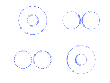
Figure 1. The images (shown right) under the forward and inverse conformal mappings of equi-spaced pre-image points on the circles on the $\zeta$ and the $z$ planes (shown left). The latter are used as collocation points for the hybrid basis scheme.

4. Exact solution

There is an exact solution, described in [6], for the two-disc problem which can be used to test the accuracy of the numerical scheme; it also forms the basis of our analysis in §6. This solution is given as follows. Define the two functions

(13) $$P(\zeta)\equiv(1-\zeta)\prod_{k=1}^{\infty}(1-\rho^{2k}\zeta)(1-\rho^{2k}\zeta^{-1}),\qquad K(\zeta)={\zeta P_{\zeta}(\zeta)\over P(\zeta)}.$$

Then the exact solution for $W(\zeta)\equiv w(z(\zeta))$, satisfying the (arbitrarily chosen) normalization that $W(-1)=0$, is

(14) $$W(\zeta)=-2AU_{0}\left(K(\sqrt{\rho}^{-1})-K(-\zeta\sqrt{\rho}^{-1})\right)+2A{\overline{U}_{0}}\left(K(\sqrt{\rho})-K(-\zeta\sqrt{\rho})\right).$$

This exact solution can be computed to arbitrary accuracy by truncating the infinite product (13) at the appropriate level. It can be shown, directly from its definition (13), that $P(\zeta,\rho)$ satisfies the functional relations

(15) $$P(\rho^{2}\zeta,\rho)=P(1/\zeta,\rho)=-\zeta^{-1}P(\zeta,\rho).$$

From these it is then easily deduced that

(16) $$K(\rho^{2}\zeta,\rho)=K(\zeta,\rho)-1,\qquad K(1/\zeta,\rho)=1-K(\zeta,\rho).$$

The identities (16) can be used to directly verify that (14) is the required solution.

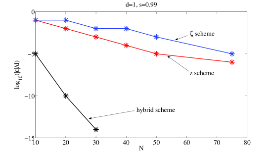
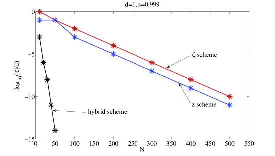
Figure 2. Comparison of the performance of the three schemes in the two-disc problem with $d=1,s=0.99$ (upper) and $d=1,s=0.999$ (lower). The logarithm of the maximum absolute error is plotted against the number of modes $N$ in the truncation.

5. Performance

To compare the performance of the three methods, the upper graph in Figure 2 shows the logarithm of the maximum absolute error in the numerical solutions compared with the exact solution plotted as a function of the truncation level $N$ for the case $d=1,s=0.99$ and $U_{0}=e^{{\rm i}\pi/4}$ so that the separation of the two discs is $0.02$. The errors were computed by calculating the difference between $w(z)$ as given by the exact solution (14) (evaluated on the boundaries of the two discs) to the values given by the numerical schemes. It is clear that, while both the $z$-scheme and $\zeta$-scheme give comparable accuracy at the same level of truncation, the hybrid scheme offers dramatic increases in accuracy at much smaller levels of truncation. This feature becomes even more pronounced at smaller separation distances: Figure 2 also shows results for $d=1,s=0.999$ and $U_{0}=e^{i\pi/4}$ so that the separation of the two discs is $0.002$, an order of magnitude smaller.

The advantages of the hybrid basis scheme are seen even more clearly in Figure 3. At each value of the disc separation (horizontal axis) the vertical axis shows the number of modes required to attain accuracy of $10^{-6}$ (as compared with the exact solution). While around $1000$ modes are needed for both the $z$-scheme and the $\zeta$-schemes in order to attain the required accuracy when the disc separation is of the order of $10^{-4}$, the hybrid scheme attains the same accuracy with only $140$ modes even when the separation is as small as $10^{-6}$. For such small separations, both the $z$-scheme and the $\zeta$-schemes become unfeasible (requiring extremely large numbers of modes, which is why the results for these methods have been omitted from Figure 3).

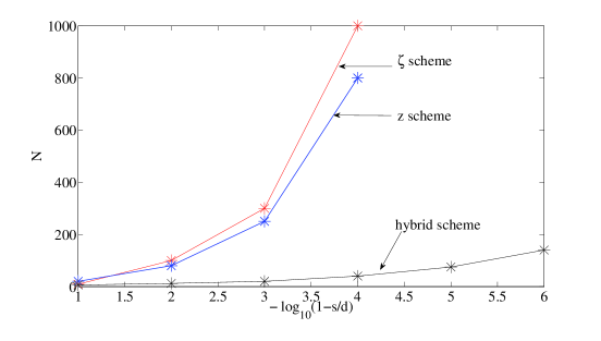
Figure 3. Comparison of the performance of the three schemes in the two-disc problem. At each value of the disc separation (horizontal axis), the vertical axis shows the number of modes required to attain accuracy of $10^{-6}$ (compared to the exact solution).

6. Two-scale analysis

The aim of this section is to demonstrate why a hybrid basis scheme involving series expansions in both the $\zeta$ and $z$ variables might be expected to perform better than separate expansions in either variable, as the foregoing numerical evidence has shown. We show the hybrid scheme has better decay properties of its coefficients than a power series in either the $\zeta$ or $z$ variables separately. We will prove the following theorem:

Theorem 1.

There exists a representation of complex potential $w$ in the following form:

(17) $$w=U_{0}z+a_{0}+\sum_{j=1}^{\infty}\left(a_{j}\zeta^{j}+b_{j}\rho^{j}\zeta^{-j}\right)+\sum_{j=1}^{\infty}\left[{c_{j}s^{j}\over(z-d)^{j}}+{d_{j}{s^{j}}\over(z+d)^{j}}\right],$$

where for any $k\geq 1$,

(18) $$j^{k}|a_{j}|\ ,j^{k}|b_{j}|\ ,j^{k}|c_{j}|\ ,j^{k}|d_{j}|\leq\frac{M_{k}}{T^{k/2+1}}\ ,$$

where $T=(1/\pi)\log\rho^{-1}$ scales as $\sqrt{1-s/d}$ and $M_{k}$ is independent of $T$. However, when either of the sets $\left\{a_{j},b_{j}\right\}$ or $\left\{c_{j},d_{j}\right\}$ is chosen to be zero, then the best possible bounds in the above scale as $1/T^{k+1}$.

Further, there exists a logarithmic decomposition in the form

(19) $$w(z)=U_{0}z+a_{0}+\sum_{j=1}^{\infty}\frac{c_{j}s^{j}}{(z-d)^{j}}+\frac{d_{j}s^{j}}{(z+d)^{j}}+\frac{A}{\pi T}\left(U_{0}-{\bar{U}}_{0}\right)\log\left[\frac{(z-d)(z+A)}{(z+d)(z-A)}\right]$$

with uniform rapid decay properties

(20) $$j^{k}|c_{j}|\ ,j^{k}|d_{j}|\leq\frac{M_{k}}{T}$$

for any $k\geq 1$.

The proof will make use of the exact solution (14) known for the two-cylinder case and the a few preliminary Lemmas and Propositions. The proof is completed in §6.6.

6.1. The function $K(\zeta,\rho)$

The exact solution (14) for the complex velocity potential is given in (14) in terms of the function $K(\zeta,\rho)$ which can be shown from its definition (13) to admit the infinite sum representation

(21) $$K(\zeta)=-\frac{\zeta}{1-\zeta}+\sum_{k=1}^{\infty}\left\{-\frac{\rho^{2k}\zeta}{1-\rho^{2k}\zeta}+\frac{\rho^{2k}\zeta^{-1}}{1-\rho^{2k}\zeta^{-1}}\right\}.$$

$K$ is single valued function of $\zeta$, implying that

(22) $$K(\zeta e^{2{\rm i}\pi})=K(\zeta),$$

while it also satisfies the “quasi-periodic” property $K(\rho^{2}\zeta,\rho)=K(\zeta,\rho)-1$ already given in (16). From these properties it should be clear that there is a connection between $K(e^{\pi\xi})$ and the quasi-periodic Weierstrass zeta function in the $\xi$ variable where

(23) $$\xi=\frac{1}{\pi}\log\zeta.$$

Moreover, its derivative is associated with the Weierstrass $\wp$ function with periods $2T:=(2/\pi)\log\rho^{-1}$ and $2{\rm i}$. Indeed on use of certain representations of the Weierstrass $\wp$ function, it is possible to show (see appendix) that

(24) $$K\left(e^{\pi\xi}\right)=\frac{\xi}{2T}+\left(\frac{1}{2}-\frac{{\rm i}}{2T}\right)+\frac{{\rm i}}{T}\left(\frac{\chi}{\chi-1}\right)+\frac{{\rm i}}{T}\sum_{m=1}^{\infty}\left(\frac{\mu^{m}\chi^{-1}}{1-\mu^{m}\chi^{-1}}-\frac{\mu^{m}\chi}{1-\mu^{m}\chi}\right),$$

where

(25) $$T=\frac{1}{\pi}\log\rho^{-1},\qquad\mu=e^{-2\pi/T},\qquad\chi=e^{{\rm i}\pi\xi/T}.$$

It follows that on the boundary $|\zeta|=1$, which corresponds to $|z-d|=s$, with parametrizations:

(26) $$\zeta=-e^{{\rm i}\nu},\qquad z=d+se^{-{\rm i}\theta},\qquad{\rm where}~{}~{}\nu,\theta\in[-\pi,\pi]\ ,$$

we obtain

(27) $$\begin{split}K\left(-\rho^{-1/2}\zeta\right)&=\frac{{\rm i}\nu}{2\pi T}+\left(\frac{3}{4}-\frac{{\rm i}}{2T}\right)+\frac{1}{T}\left(\frac{e^{-\nu/T}}{1-{\rm i}e^{-\nu/T}}\right)\\ &+\frac{1}{T}\sum_{m=1}^{\infty}\left(\frac{\mu^{m}e^{\nu/T}}{1+{\rm i}\mu^{m}e^{\nu/T}}+\frac{\mu^{m}e^{-\nu/T}}{1-{\rm i}\mu^{m}e^{-\nu/T}}\right),\\ K\left(-\rho^{1/2}\zeta\right)&=\frac{{\rm i}\nu}{2\pi T}+\left(\frac{1}{4}-\frac{{\rm i}}{2T}\right)-\frac{1}{T}\left(\frac{e^{-\nu/T}}{1+{\rm i}e^{-\nu/T}}\right)\\ &-\frac{1}{T}\sum_{m=1}^{\infty}\left(\frac{\mu^{m}e^{\nu/T}}{1-{\rm i}\mu^{m}e^{\nu/T}}+\frac{\mu^{m}e^{-\nu/T}}{1+{\rm i}\mu^{m}e^{-\nu/T}}\right).\end{split}$$

The relationship between angles $\nu$ and $\theta$ in the $z$ and $\zeta$ domains are given by

(28) $$\nu=2\arctan\left[\left(\frac{1-\sqrt{\rho}}{1+\sqrt{\rho}}\right)\tan\frac{\theta}{2}\right],\qquad\theta=2\arctan\left\{\left(\frac{1+\sqrt{\rho}}{1-\sqrt{\rho}}\right)\tan\frac{\nu}{2}\right\}.$$

Similarly, on $|\zeta|=\rho$, corresponding to $|z+d|=s$, with parameterization

(29) $$\zeta=-\rho e^{{\rm i}\nu},\qquad z=-d-se^{{\rm i}\theta},\qquad{\rm where}~{}\nu,\theta\in[-\pi,\pi],$$

we obtain the same relationship (28) between angles $\nu$ and $\theta$ as before, while

(30) $$\begin{split}K\left(-\rho^{-1/2}\zeta\right)&=\frac{{\rm i}\nu}{2\pi T}+\left(\frac{1}{4}-\frac{{\rm i}}{2T}\right)-\frac{1}{T}\left(\frac{e^{-\nu/T}}{1+{\rm i}e^{-\nu/T}}\right)\\ &-\frac{1}{T}\sum_{m=1}^{\infty}\left(\frac{\mu^{m}e^{\nu/T}}{1-{\rm i}\mu^{m}e^{\nu/T}}+\frac{\mu^{m}e^{-\nu/T}}{1+{\rm i}\mu^{m}e^{-\nu/T}}\right),\\ K\left(-\rho^{1/2}\zeta\right)&=\frac{{\rm i}\nu}{2\pi T}+\left(-\frac{1}{4}-\frac{{\rm i}}{2T}\right)+\frac{1}{T}\left(\frac{e^{-\nu/T}}{1-{\rm i}e^{-\nu/T}}\right)\\ &+\frac{1}{T}\sum_{m=1}^{\infty}\left(\frac{\mu^{m}e^{\nu/T}}{1+{\rm i}\mu^{m}e^{\nu/T}}+\frac{\mu^{m}e^{-\nu/T}}{1-{\rm i}\mu^{m}e^{-\nu/T}}\right).\end{split}$$

We note that in particular on each of the circles $|\zeta|=1$ and $|\zeta|=\rho$, we have ${\rm i}\zeta\partial_{\zeta}K\left(-\rho^{-1/2}\zeta\right)=\partial_{\nu}K\left(-\rho^{-1/2}\zeta\right)$ involves exponential terms in $\nu/T$ that tends to the same constant – namely, ${{\rm i}}/[{2\pi T}]$ – exponentially outside an $O(T)$ neighborhood of $\nu=0$. Because of the $\nu=O(T)$ scale, it is clear also that this a series representation in the form $W-U_{0}z=\sum_{k}\left(a_{j}\zeta^{j}+b_{j}\rho^{j}\zeta^{-j}\right)$ will have poor decay properties; indeed since bounds on each of $\partial_{\nu}^{k}\left(W(-e^{i\nu})-U_{0}Z(-e^{i\nu})\right)$ $\partial_{\nu}^{k}\left(W(-\rho e^{i\nu})-U_{0}Z(-\rho e^{i\nu})\right)$ scales as $T^{-k-1}$, from well-known properties of Fourier coefficients, it follows we will obtain poor estimates $j^{k}|a_{j}|\ ,j^{k}|b_{j}|\leq M_{k}/T^{k+1}$. We now seek to alleviate this through use of a hybrid representation.

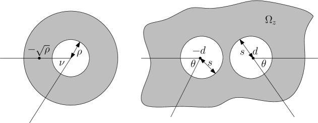
Figure 4. Definition sketch for the angles $\nu$ and $\theta$ in (26) and (29). The annulus $\rho<\zeta<1$ and the region exterior to the two discs centred at $z=\pm d$ are shown shaded.

6.2. The function $\omega(z)$ and rapidly decaying series

Definition 1.

Define

(31) $$\omega(z)=\frac{1}{\zeta z_{\zeta}}\left\{\zeta W_{\zeta}(\zeta(z))-U_{0}\zeta z_{\zeta}-\frac{A}{\pi T}(U_{0}-{\bar{U}}_{0})\right\}$$

Remark 1.

On use of (14) and (31) we find

(32) $$\omega(z)=\frac{dW}{dz}-U_{0}-\frac{A(U_{0}-{\bar{U}}_{0})}{\pi T\zeta z_{\zeta}}=\frac{dW}{dz}-U_{0}+\frac{2A^{2}(U_{0}-{\bar{U}}_{0})}{\pi T(z^{2}-A^{2})}.$$

It is important to note that the two points $z=\pm{A}$ lie outside the domain $\Omega_{z}:=\left\{z:|z+d|\geq s,|z-d|\geq s\right\}$. It follows that $\omega$ is analytic in $\Omega_{z}$ with $\omega\rightarrow 0$ as $z\rightarrow\infty$. Therefore,

(33) $$\omega(z)=\sum_{j=1}^{\infty}\frac{c_{j}s^{j}}{(z-d)^{j}}+\sum_{j=1}^{\infty}\frac{d_{j}s^{j}}{(z+d)^{j}}\ ,$$

where

(34) $$c_{j}=-\frac{1}{2\pi{\rm i}s^{j}}\oint_{|z^{\prime}-d|=s}\omega(z^{\prime})(z^{\prime}-d)^{j-1}dz^{\prime}=\frac{1}{2\pi}\int_{-\pi}^{\pi}\omega(d+se^{-{\rm i}\theta^{\prime}})e^{-{\rm i}j\theta^{\prime}}d\theta^{\prime}$$

(35) $$d_{j}=-\frac{1}{2\pi{\rm i}s^{j}}\oint_{|z^{\prime}+d|=s}\omega(z^{\prime})(z^{\prime}+d)^{j-1}dz^{\prime}=\frac{(-1)^{j}}{2\pi}\int_{-\pi}^{\pi}\omega(-d-se^{{\rm i}\theta^{\prime}})e^{{\rm i}j\theta^{\prime}}d\theta^{\prime}$$

and where contour integration in the $z^{\prime}$ plane is understood in a clockwise sense

On $z=d+se^{-{\rm i}\theta}$, corresponding to $\zeta=-e^{{\rm i}\nu}$, (32) implies

(36) $$\omega(z)=-U_{0}+\frac{2{\rm i}AU_{0}\nu_{\theta}}{(z-d)}\left[\partial_{\nu}K(-\rho^{-1/2}\zeta)-\frac{{\rm i}}{2\pi T}\right]\\ -\frac{2A{\rm i}{\bar{U}}_{0}\nu_{\theta}}{(z-d)}\left[\partial_{\nu}K(-\rho^{1/2}\zeta)-\frac{{\rm i}}{2\pi T}\right],$$

and on $z=-d-se^{{\rm i}\theta}$, corresponding to $\zeta=-\rho e^{{\rm i}\nu}$, (32) implies

(37) $$\omega(z)=-U_{0}-\frac{2{\rm i}AU_{0}\nu_{\theta}}{(z+d)}\left[\partial_{\nu}K(-\rho^{-1/2}\zeta)-\frac{{\rm i}}{2\pi T}\right]\\ +\frac{2{\rm i}A{\bar{U}}_{0}\nu_{\theta}}{(z+d)}\left[\partial_{\nu}K(-\rho^{1/2}\zeta)-\frac{{\rm i}}{2\pi T}\right].$$

In particular integration in (34)-(35) for $j=1$ is explicit resulting in

(38) $$sc_{1}=\frac{A}{\pi T}(U_{0}-{\bar{U}}_{0})=-sd_{1}.$$

Further, it is clear from (31) that

(39) $$W(z)=C\int^{z}\omega(z^{\prime})dz^{\prime}+\frac{A}{\pi T}(U_{0}-{\bar{U}}_{0})\log\left(\frac{z+A}{z-A}\right)$$

implying from (33) and (38) that for some constant $C$

(40) $$W=C-\sum_{k=2}^{\infty}\frac{s^{k}c_{k}}{(k-1)(z-d)^{k-1}}-\sum_{k=2}^{\infty}\frac{s^{k}d_{k}}{(k-1)(z+d)^{k-1}}+W_{2},$$

where

(41) $$W_{2}(z)=\frac{A}{\pi T}(U_{0}-{\bar{U}}_{0})\log\left(\frac{z-d}{z-A}\right)+\frac{A}{\pi T}(U_{0}-{\bar{U}}_{0})\log\left(\frac{z+A}{z+d}\right).$$

We will now prove that the Laurent series coefficients of $\omega(z)$, namely $\{c_{k}\}$, $\{d_{k}\}$, decay rapidly in $k$ uniformly for $T\in(0,T_{0}]$ in the following sense:

Proposition 2.

For any integer $k\geq 0$,

(42) $$\Big{|}j^{k}c_{j}\Big{|}\ ,\Big{|}j^{k}d_{j}\Big{|}\leq\frac{M_{k}}{T}$$

where $M_{k}$ is independent of $T\in(0,T_{0}]$.

Remark 2.

From (34), (35), (36) and (37), the proof of Proposition 2 will follow after we show that on each of the boundaries $\zeta=-e^{{\rm i}\nu(\theta)}$ and $\zeta=-\rho e^{{\rm i}\nu(\theta)}$, for any integer $k\geq 0$

(43) $$T\partial_{\theta}^{k+1}\left(K(-\rho^{-1/2}\zeta)-\frac{{\rm i}\nu}{2\pi T}\right),\qquad T\partial_{\theta}^{k+1}\left(K(-\rho^{1/2}\zeta)-\frac{{\rm i}\nu}{2\pi T}\right)$$

are each $2\pi$-periodic function of $\theta$ and have bounds $M_{k}$ independent of $T$. Periodicity is clear since, from (27) and (30), both

(44) $${\partial\over\partial\theta}\left[K(-\rho^{-1/2}\zeta)-\frac{{\rm i}\nu}{2\pi T}\right],\qquad{\rm and}\qquad{\partial\over\partial\theta}\left[K(-\rho^{1/2}\zeta)-\frac{{\rm i}\nu}{2\pi T}\right]$$

are obviously periodic in $\nu$ for $\zeta=-e^{{\rm i}\nu},-\rho e^{{\rm i}\nu}$, and therefore in $\theta$; derivatives of $\nu$ are also periodic in $\theta$ as is clear from (28). Hence, we only need to prove the bounds.

Remark 3.

We will find the following identity on derivativies of smooth composite functions useful:

(45) $$\partial_{\theta}^{l}F(\eta(\theta))=\sum_{j_{m}\geq 0\atop\sum_{m=1}^{l}mj_{m}=l}C_{j_{1},j_{2},\cdots,j_{l}}\left(\partial_{\eta}^{(\sum_{m=1}^{l}j_{m})}F\right)\left(\prod_{m=1}^{l}\left[\partial_{\theta}^{m}\eta\right]^{j_{m}}\right),$$

Lemma 3.

For $T\in(0,T_{0}]$, define

(46) $$\chi=\exp\left[-\frac{2}{T}\arctan\left(\frac{1-\sqrt{\rho}}{1+\sqrt{\rho}}\tan\frac{\theta}{2}\right)\right].$$

Then, for $\theta\in[0,\pi)$,

(47) $$\Big{|}\partial_{\theta}^{l}\chi\Big{|}\leq M_{l}$$

where constant $M_{l}$ is independent of $T$ and is only dependent on $l$.

Proof.

In the following proof, $C_{l}$ is a generic constant depending on $l$ that is allowed to vary from step to step. We introduce for convenience intermediate variables $x=\tan(\theta/2)$, $y=c_{0}Tx$ and $\nu_{1}=(1/T)\arctan y$; it follows from (46) that

(48) $$\chi=e^{-2\nu_{1}}.$$

First, consider the case when $xT^{2/3}\leq 1$, implying $y$ is small. Taylor expansion of $\arctan y$ gives

(49) $$\nu_{1}=c_{0}x+\sum_{j=3}^{\infty}(-1)^{j}jT^{j-1}c_{0}^{j}\frac{x^{j}}{j}$$

We note that for any $\theta\in[0,\pi)$, $|\partial_{\theta}^{j}x|\leq C(1+x)^{j+1}$. Identifying $\eta$ with $x$ and $F$ with $c_{0}^{j}T^{j-1}x^{j}$ in (45) to determine bounds on the sum in (49), it follows that for $xT^{2/3}\leq 1$,

(50) $$\Big{|}\partial_{\theta}^{l}\nu_{1}\Big{|}\leq C_{l}(1+x)^{l+1}\left(1+\sum_{j=3}^{\infty}T^{j-1}c_{0}^{j}x^{j}\right)\leq C_{l}(1+x)^{l+1}\leq C_{l}(1+\nu_{1})^{l+1}$$

Now identifying $\eta$ with $\nu_{1}$ and taking $F(\nu_{1})=e^{-2\nu_{1}}$ in (45) and using (50), it follows that

(51) $$\Big{|}\partial_{\theta}^{l}e^{-2\nu_{1}}\Big{|}\leq C_{l}e^{-2\nu_{1}}(1+\nu_{1})^{2l}\leq C_{l}$$

Now consider, $T^{-2/3}\leq x\leq\frac{4}{c_{0}T}$, i.e. $c_{0}T^{1/3}\leq y\leq 4$. We note that

(52) $$\left|{\partial^{l}y\over\partial\theta^{l}}\right|=c_{0}T\left|{\partial^{l}x\over\partial\theta^{l}}\right|\leq C_{l}T(1+x)^{l+1}$$

Identifying $\eta$ with $y$, and taking $F(y)=\arctan(y)$ in (45), it follows from (52) that for $y\leq 4$,

(53) $$\Big{|}\partial_{\theta}^{l}\nu_{1}\Big{|}\leq\frac{C_{l}}{T}(1+x)^{l}$$

Now, identifying $\nu_{1}$ with $\eta$ and taking $F(\nu_{1})=e^{-2\nu_{1}}$ in (45), and noting $y\geq c_{0}T^{1/3}$ implies $\nu_{1}\geq\frac{1}{T}\arctan[c_{0}T^{1/3}]$, it follows from (53):

(54) $$\Big{|}\partial_{\theta}^{l}e^{-2\nu_{1}}\Big{|}\leq\frac{C_{l}}{T^{l}}(1+x)^{l}e^{-2\nu_{1}}\leq C_{l}$$

since $y\leq 4$ implies $x^{l}\leq\frac{4^{l}}{(c_{0}T)^{l}}$. For $y\geq 4$, note the the convergent series representation in powers of $\frac{1}{y}$

(55) $$\nu_{1}=\frac{1}{T}\left(\frac{\pi}{2}-\sum_{j=0}^{\infty}\frac{(-1)^{j}}{(2j+1)y^{2j+1}}\right)=:\frac{1}{T}f\left(\frac{1}{y}\right)$$

We also note that

(56) $$\frac{1}{y}=\frac{1}{c_{0}T}\cot\frac{\theta}{2}$$

and the mapping $\theta\rightarrow Ty^{-1}$ is smooth for $y\geq 4$. Identifying $\frac{1}{y}$ with $\eta$ and $F$ with $\frac{1}{T}f$ in (45), it follows from (56) that

(57) $$\Big{|}\partial_{\theta}^{l}\nu_{1}\Big{|}\leq\frac{C_{l}}{T^{l+1}}$$

On the otherhand if $y\geq 4$, then $e^{-2\nu_{1}}\leq e^{-\frac{2}{T}\arctan 4}$ and therefore, using (45) again

(58) $$\Big{|}\partial_{\theta}^{l}e^{-2\nu_{1}}\Big{|}\leq\frac{C_{l}e^{-\frac{2}{T}\arctan 4}}{T^{2l}}\leq C_{l}$$

Hence the lemma follows for all cases.     

Lemma 4.

For $T\in(0,T_{0}]$, define

$$F_{0}(\nu)=\frac{e^{-\nu/T}}{1\pm{{\rm i}}e^{-\nu/T}},\qquad F_{1}(\nu)=\frac{\mu e^{\pm{\nu}/T}}{1+{\rm i}\mu^{m}e^{\pm{\nu}/T}},\qquad F_{2}(\nu)=\frac{\mu e^{\pm{\nu}/T}}{1-{\rm i}\mu^{m}e^{\pm{\nu}/T}}.$$

For $j=0,1,2$, for any integer $l\geq 1$, there exists constant $M_{l}$ independent of $T$ so that for $\nu\in\left(-\pi,\pi\right)$,

(59) $$\Big{|}\partial_{\theta}^{l}F_{j}(\nu)\Big{|}\leq M_{l}.$$

Proof.

Consider first $F_{0}$. Since use of the transformation $\nu\rightarrow-\nu$ in the alternate form

(60) $$F_{0}=\mp{{\rm i}}-\frac{e^{\nu/T}}{1\mp{{\rm i}}e^{\nu/T}}$$

makes the arguments for $\nu\in\left(-\pi,0\right]$ equivalent to those for $\nu\in\left[0,\pi\right)$ then we restrict to the latter case. Since $F_{0}$ is a rational function of $\chi=e^{-\nu/T}$ with singularity location in the complex plane at $O(1)$ distance, and with all derivatives with respect to $\chi$ bounded for $\chi\in[0,\infty)$, it suffices to show that $\Big{|}\partial_{\theta}^{l}\chi\Big{|}\leq C_{l}$, with $C_{l}$ independent of $T$. But this has been proved in Lemma 3. The argument for each of $F_{1}$ and $F_{2}$ is similar, except that we need to use

$$\Big{|}\mu e^{\nu_{1}}\partial^{k}_{\theta}\nu_{1}\Big{|}\leq C_{0}e^{-2\pi/T}\nu_{1}^{k+1}e^{\nu_{1}}\leq M_{k},$$

independent of $T$.     

Proof of Proposition 2: From Remark 2, it is enough to obtain bounds independent of $T$ for terms appearing in 43 on each circle $\zeta=-e^{{\rm i}\nu(\theta)}$ and $\zeta=-\rho e^{{\rm i}\nu(\theta)}$. However, from (27) and (30), it is clear from applying Lemma 4 on each term that this is true and the proof of Proposition 2 follows after use of dominated convergence theorem to justify the commutation of infinite sum with derivatives in $\theta$.

Remark 4.

Note that the second part of Theorem 1 on the logarithmic decomposition is now obvious from Proposition 2 and on use of (40) and (41).

6.3. Series representation of $W_{2}$

Note from (41) that

(61) $$W_{2}(z)=-\frac{A}{\pi T}\left(U_{0}-{\bar{U}}_{0}\right)W_{2,1}(z)+\frac{A}{\pi T}\left(U_{0}-{\bar{U}}_{0}\right)W_{2,2}(z)$$

where

(62) $$W_{2,1}(z)=\log\left(\frac{z-A}{z-d}\right)=\log\left(1+\frac{\sqrt{\rho}s}{z-d}\right)$$

(63) $$W_{2,2}(z)=\log\left(\frac{z+A}{z+d}\right)=\log\left(1-\frac{\sqrt{\rho}s}{z+d}\right)$$

We note that $W_{2,1}$ is an analytic function outside the circle $|z-d|=s$, whose Laurent series in powers of ${s}/({z-d})$ has a radius of convergence $\rho^{-1/2}$, while $W_{2,2}$ is an analytic function outside $|z+d|=s$, whose Laurent series in powers of ${s}/({z+d})$ also has a radius of convergence $\rho^{-1/2}$. If we use (7)-(8), then it is clear that

(64) $$W_{2,1}(Z(\zeta))=-\log\left(\frac{d+A}{2A}\right)-\log\left(1+\rho^{1/2}\zeta\right)$$

The radius of convergence in powers of $\zeta$ for the analytic function $W_{2,1}(Z(\zeta))$ inside the unit circle is again $\rho^{-1/2}$ and there is no advantage using the $\zeta$ scheme versus the $z$ scheme. Also,

(65) $$W_{2,2}(Z(\zeta))=-\log\left(\frac{d+A}{2A}\right)-\log\left(1+\rho^{3/2}\zeta^{-1}\right)$$

and, again, the radius of convergence of a series in $\rho/\zeta$ of this analytic function in $|\zeta|>\rho$ is $\rho^{-1/2}$ and there is no advantage using the $\zeta$ scheme over the $z$ scheme. When $\rho$ is very close to 1, the geometric decay factor is poor and one needs a large number of terms in the series represention for each of $W_{2,1}$ and $W_{2,2}$. Indeed, note that on the circle $\zeta=-e^{i\nu}$,

(66) $$\Big{|}\partial_{\nu}^{k}W_{2,1}\left(Z(-e^{-i\nu})\right)\Big{|}\leq C_{0}T^{-k}\ ,$$

which is reflected in the Taylor series coefficient of $W_{2,1}(\zeta)=\sum_{j=0}^{\infty}w_{j}\zeta^{j}$ in the observation

(67) $$j^{k}|w_{j}|=\frac{j^{k}}{j}\rho^{1/2j}=j^{k-1}e^{-\pi Tj/2}\leq C_{0}T^{-(k-1)}.$$

From the logarithmic expansion in (62) in powers of $s/(z-d)$, i.e., $W_{2,1}=\sum_{k=1}^{\infty}\frac{W_{j}s^{j}}{(z-d)^{j}}$, we also have

(68) $$j^{k}|W_{j}|\leq C_{0}T^{-(k-1)}.$$

Similar statements hold for series expansions of $W_{2,2}$ in powers of $\rho/\zeta$ or $s/(z+d)$.

We now seek to prove that the hybrid basis scheme does better than (67) or (68). We demonstrate this only for $W_{2,1}$ since an analogous construction is possible for $W_{2,2}$, with $s/(z-d)$ replaced by $s/(z+d)$ and $\zeta$ replaced by $\rho/\zeta$ in the series representation.

6.4. Hybrid decomposition of $W_{2,1}$

To be more precise, we prove the following theorem:

Proposition 5.

There exists decomposition of

(69) $$W_{2,1}=\omega_{1}(\zeta)+\omega_{2}\left(\frac{s}{z-d}\right)~{}\ ,~{}W_{2,2}=\omega_{3}(\rho\zeta^{-1})+\omega_{4}\left(\frac{s}{z+d}\right)\ ,$$

where each of $\omega_{1}$, $\omega_{2}$, $\omega_{3}$ and $\omega_{4}$ are analytic when its argument is inside the unit circle and for any $m=1,2,3,4$,

(70) $$\omega_{m}(\eta)=\sum_{j=0}^{\infty}a_{j,m}\eta^{j}$$

such that for any integer $k\geq 1$,

(71) $$\Big{|}j^{k}a_{j,m}\Big{|}\ \leq\frac{M_{k}}{T^{k/2}},$$

where $M_{k}$ is independent of $j$ and $T$, (i.e. of $\rho$)).

The proof of Proposition 5 will await preliminary Lemmas that pertain to construction of the decomposition of $W_{2,1}$ into $\omega_{1}$ and $\omega_{2}$ and smoothness properties of each the $\nu$ and $\theta$ representations on the circular boundaries and uniform control of all derivatives as $T\rightarrow 0^{+}$ ($\rho\rightarrow 1^{-}$). The arguments are nearly identical for $W_{2,2}$.

6.5. Construction of $\omega_{1}$, $\omega_{2}$, Proof of Proposition 5 and Theorem 1

Definition 6.

We choose $\delta$ that shrinks with $T$ as $T\rightarrow 0$ so as to satisfy $1>>\delta>>T^{1-\epsilon_{1}}$ for some $1>\epsilon_{1}>0$ independent of $T$. A more precise choice will be made later to optimize the decay rate of power series. We define an even, smooth, cut-off function $\Phi\in{\bf C}^{\infty}[-\pi,\pi]$ so that

(72) $$\Phi(\nu)=1~{}~{}{\rm for}~{}|\nu|\leq\delta\ ,\Phi(\nu)=0~{}~{}{\rm for}~{}|\nu|\in[2\delta,\pi]$$

and with property $\Big{|}\partial_{\nu}^{l}\Phi(\nu)\Big{|}\lesssim\delta^{-l}$. There are standard choices for such functions (see Evans PDE book for instance). Corresponding to such a choice of $\Phi$, we define a single valued analytic function $\omega_{1}(\zeta)$ analytic in $|\zeta|<1$ such that on the boundary $|\zeta|=1$ with representation $\zeta=-e^{{\rm i}\nu}$, $\nu\in[-\pi,\pi]$

(73) $$\mathrm{Re}~{}\omega_{1}(-e^{{\rm i}\nu})=\left(1-\Phi(\nu)\right)\mathrm{Re}~{}W_{2,1}\left(Z(-e^{{\rm i}\nu})\right)$$

We define an analytic function $\omega_{2}(\zeta)$ analytic in $|\zeta|<1$ so that on $\zeta=-e^{{\rm i}\nu}$

(74) $$\mathrm{Re}~{}\omega_{2}(-e^{{\rm i}\nu})=\Phi(\nu)~{}\mathrm{Re}~{}W_{2,1}\left(Z(-e^{{\rm i}\nu})\right)$$

Lemma 7.

Define $H(\nu)=\left(1-\Phi(\nu)\right)\mathrm{Re}~{}W_{2,1}\left(Z(-e^{{\rm i}\nu})\right)$. $H$ may be extended to be a smooth $2\pi$-periodic function of $\nu$ satisfying

(75) $$\Big{|}\partial_{\nu}^{k}H(\nu)\Big{|}\leq\frac{M_{k}}{\delta^{k}},$$

where $M_{k}$ may be chosen independent of $\delta$ and $T$ ($\rho$).

Proof.

Since $1-\Phi$ is a smooth cut-off function with support in $\pi\geq|\nu|\geq\delta$ and $1-\Phi=1$ for $\pi\geq|\nu|\geq 2\delta$, the $2\pi$ periodicity and smoothness of $\log(1-\rho^{-1/2}e^{i\nu})$ translates into smoothness of $H$ with $\partial_{\nu}^{k}H(\pi)=\partial_{\nu}^{k}H(-\pi)$ for any integer $k\geq 0$. We only need to show the bounds. We note that $\Big{|}\delta^{j}\partial_{\nu}^{j}\Phi\Big{|}\leq c_{0}$, independent of $T$ and $\delta$, and for $|\nu|\in[\delta,\pi]$, for $k\geq 1$,

(76) $$\delta^{k}\Big{|}\partial_{\nu}^{k}\log\left(1-\rho^{-1/2}e^{i\nu}\right)\Big{|}\leq C_{0}$$

Therefore, from a Leibnitz representation of the derivatives of a product, the Lemma follows immediately.     

Proposition 8.

$\omega_{1}$ defined in Definition 6 with representation

(77) $$\omega_{1}(\zeta)=\sum_{j=0}^{\infty}a_{j}\zeta^{j}$$

satisfies

(78) $$j^{k}|a_{j}|\leq M_{k}/\delta^{k}$$

for any $k\geq 1$, where $M_{k}$ is independent of $\delta$ and $T$.

Proof.

We simply note that on the boundary $\zeta=-e^{{\rm i}\nu}$, from the Fourier representation and noting that $H$ is even we have

(79) $$\mathrm{Re}~{}\omega_{1}\left(-e^{{\rm i}\nu}\right)=H(\nu)=\sum_{j=0}^{\infty}(-1)^{j}a_{j}\cos(j\nu),$$

where previous Lemma implies

(80) $$j^{k}|a_{j}|\leq M_{k}/\delta^{k}.$$

Hence the Lemma follows since (79) implies (77) because $\mathrm{Im}[\omega_{1}(0)]=0$.     

We now consider the problem of representing $\omega_{2}$. Note that on $\zeta=-e^{{\rm i}\nu}$

(81) $$\mathrm{Re}~{}\omega_{2}\left(\boldsymbol{\zeta}(d+se^{-{\rm i}\theta})\right)=\Phi(\nu(\theta))\log\left(1+\rho^{-1/2}e^{{\rm i}\theta}\right).$$

Define

(82) $$\theta_{m}=2\arctan\left\{\left(\frac{1+\sqrt{\rho}}{1-\sqrt{\rho}}\right)\tan\delta\right\}.$$

From relation (28) between $\nu$ and $\theta$, $\Phi(\nu(\theta))=0$ for $|\theta|>\theta_{m}$. Also, $1\gg\delta\gg T$ implies that

(83) $$\theta_{m}=\pi-\frac{2}{\tan\delta}\left(\frac{1-\sqrt{\rho}}{1+\sqrt{\rho}}\right)+O(T^{3}/\delta^{3}).$$

Lemma 9.

Consider the change of variable $\nu=\nu(\theta)$ defined by (28). For $\nu\in[-2\delta,2\delta]$, i.e. $\theta\in[-\theta_{m},\theta_{m}]$, where there exists constant $C_{0}$ independent of $T$ and $\delta$ so that

(84) $$\Big{|}\partial_{\theta}^{k}\nu\Big{|}\leq C_{0}\frac{\delta^{k+1}}{T^{k}}.$$

Proof.

It is convenient to introduce the intermediate variables

(85) $$x=\tan\left(\frac{\theta}{2}\right),\qquad y=\left(\frac{1+\sqrt{\rho}}{1-\sqrt{\rho}}\right)x.$$

Then $\nu=2\arctan y$. Since $\delta$ is small, it follows that $y$, which is at most $O(\delta)$ is also small for $\theta\in[-\theta_{m},\theta_{m}]$. It immediately follows that all derivatives of $\nu$ with respect to $y$ are bounded independent of any parameter. Now consider $x=x(\theta))$. Clearly derivatives of $x(\theta)$ can only be large for $|\theta|$ near $\pi$, where there is a simple pole. It follows that $\Big{|}\partial_{\theta}^{l}x\Big{|}\leq c_{0}x^{l+1}$. Therefore, $\Big{|}\partial_{\theta}^{k}y\Big{|}\leq c_{0}Tx^{k+1}\leq c_{0}y^{k+1}/T^{k}$. Since $y=O(\delta)$, the Lemma immediately follows.     

Lemma 10.

For the cut-off function $\Phi$ as defined earlier, with $\theta\in[-\theta_{m},\theta_{m}]$, for any integer $k$, there exists constant $c_{0}$ independent of $\delta$ and $T$ so that

(86) $$\Big{|}\partial_{\theta}^{k}\Phi(\nu(\theta))\Big{|}\leq c_{0}\frac{\delta^{k}}{T^{k}}.$$

Proof.

We simply make use of (45) and invoke the previous Lemma and the bounds $\Big{|}\partial_{\nu}^{l}\Phi\Big{|}\leq C\delta^{-l}$.     

Lemma 11.

(87) $$H_{2}(\theta)=\mathrm{Re}~{}\omega_{2}\left(-e^{i\nu(\theta)}\right)=\Phi(\nu(\theta))\mathrm{Re}~{}\log\left(1+\rho^{1/2}e^{i\theta}\right)$$

Then for any $k\geq 1$, for $\theta\in[-\pi,\pi]$,

(88) $$\Big{|}\partial_{\theta}^{k}H_{2}(\theta)\Big{|}\leq c_{0}\frac{\delta^{k}}{T^{k}}$$

Proof.

We note that since the support of $\Phi(\nu(\theta))$ is $|\theta|\leq\theta_{m}$ and $\pi-\theta_{m}=O\left(\frac{T}{\delta}\right)$, and the observation that for $\theta\in[-\theta_{m},\theta_{m}]$,

$$\Big{|}\partial_{\theta}^{k}\log\left(1+\rho^{1/2}e^{i\theta}\right)\Big{|}\leq M_{k}\frac{\delta^{k}}{T^{k}}$$

for $M_{k}$ independent of $T$ and $\delta$. Using the Leibnitz rule, and Lemma 10, the present Lemma follows.     

Proposition 12.

The analytic function $\omega_{2}$ in $|\zeta|<1$, i.e. $|z-d|>s$ has the representation

(89) $$\omega_{2}\left(\boldsymbol{\zeta}(z)\right)=\sum_{j=0}^{\infty}\frac{b_{j}s^{j}}{(z-d)^{j}}\ ,$$

where for any $k\geq 1$,

(90) $$j^{k}|b_{j}|\leq\frac{M_{0}\delta^{k}}{T^{k}}.$$

Proof.

We use the fact that $\mathrm{Re}~{}\omega\left(\boldsymbol{\zeta}(z)\right)=H_{2}(\theta)$ and from the previous Lemma

(91) $$H_{2}(\theta)=\sum_{j=0}^{\infty}b_{j}\cos(j\theta)$$

where $b_{j}$ satisfies (90). Therefore, the proposition immediately follows.     

6.6. Proofs of Proposition 5 and Theorem 1

The proof of Proposition 5 follows from Propositions 8 and 12 if we choose $\delta=T^{1/2}$ and note that from the definition of $\omega_{1}$ and $\omega_{2}$, on $|\zeta|=1$, $\mathrm{Re}~{}W_{2,1}=\mathrm{Re}~{}\omega_{1}+\mathrm{Re}~{}\omega_{2}$ and therefore for $W_{2,1}=\omega_{1}+\omega_{2}$ since the ambiguity in the imaginary constant is resolved by the condition $\mathrm{Im}W_{2,1}(0)=0$.

The argument for $W_{2,2}$ similar except for replacing $\zeta$ by $\rho/\zeta$ and $s/(z-d)$ by $s/(z+d)$ in the arguments given already in the decomposition of $W_{2,1}$.

Proof of Theorem 1 follows by using Proposition 5 and the prior observation on the series decay for $W_{2,1}$ when a series just in $\zeta$ (or $s/(z-d)$) is used (see (67)-(68)). Similar statement hold for $W_{2,2}$ in powers either in $\rho/\zeta$ or (or $s/(z+d)$).

7. Connections with other methods

It is natural to enquire as to the connection of this method with the rather different scheme proposed by Cheng and Greengard [4]. For the two disc problem, in order to attain accuracy of ${\mathcal{O}}(10^{-6})$, Cheng and Greengard [4] use a representation of the potential fields that involves a sum of multipole expansions about 14,000 reflection points – or “images” – inside the discs. Despite this large number of multipole contributions, the total number of unknowns associated with each disc is kept small because (analytically) known reflection operators are used to generate successive generations of multipole expansions given only the parent coefficients. These reflection operators are, however, highly specific to the particular problem being solved there and are not generally applicable to other problems. We discuss this again later. In principle, successive reflections between the two discs produces an infinite number of possible image singularities about which, following Cheng & Greengard [4], one could introduce multipole expansions to improve accuracy. These image points tend to definite limit points. Explicit formulae for these limit points are given in equation (17) of [4]: if $z_{1}$ and $z_{2}$ denote the complex positions of the disc centres then the two limit points are

(92) $$z_{1}(\infty)={z_{1}+z_{2}\over 2}-\sqrt{s\hat{d}+\hat{d}^{2}/4}\left({z_{2}-z_{1}\over|z_{2}-z_{1}|}\right),$$

where $s$ is the disc radius and $\hat{d}=|z_{2}-z_{1}|-2s$ is the distance between the two discs. Careful inspection of (9) and (12) reveals that the method we have introduced here is essentially equivalent to the sum of just four multipole expansions – two about the centres of the discs and two more about the points $\pm A$. Use of (92) then reveals that our hybrid method corresponds to using multipole expansions about the two centres of the discs and their limit points after infinitely many reflections. Figure 5 illustrates the connection between the two methods schematically in the case of the two-disc problem.

The evidence here suggests that, from a numerical standpoint, it is satisfactory to use multipole expansions only about the disc centres and the limiting image points of these centres rather than using increasingly many multipole expansions about successive images.

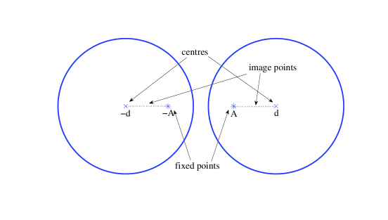
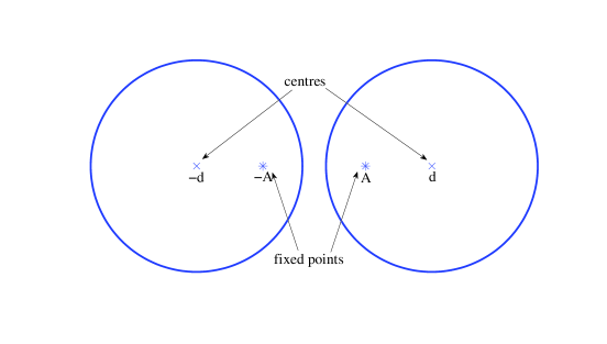
Figure 5. Schematic illustrating that the method of Cheng & Greengard [4] (upper figure) incorporates multipole expansions about successive reflections (“images”) of the circle centres in the circle boundaries. The new method (lower figure) effectively includes only multipole expansions about the circle centres and the limit points of the reflections.

8. Extension to any number of discs

Our essential idea is readily extendible to the multi-disc case. Suppose that discs $D_{i}$ and $D_{j}$ are separated by less than some threshold value $\delta$. Based on the two-disc problem just analyzed, and depending on the required accuracy and speed, an appropriate $\delta$ might be of the order ${\mathcal{O}}(10^{-2})$, for example. The conformal mapping from a concentric annulus $\rho_{ij}<|\zeta|<1$ (for some real parameter $0<\rho_{ij}<1$) to the exterior of these two discs is then found analytically. This is a Möbius transformation, as is its inverse mapping, which we will denote by $\zeta_{ij}(z)$. Then, in addition to Fourier-Laurent expansions about the disc centres, terms of the form

(93) $$\sum_{k=1}^{\mathcal{N}}c_{k}^{(ij)}[\zeta_{ij}(z)]^{k}+\sum_{k=1}^{\mathcal{N}}{d_{k}^{(ij)}\rho_{ij}^{k}\over[\zeta_{ij}(z)]^{k}}$$

are also included (additively) in the representation of the complex potential function $w(z)$. Equations for the additional coefficients $\{c_{k}^{(ij)},d_{k}^{(ij)}|k=1,...,{\mathcal{N}}\}$ are obtained, as before, by substituting the expression for $w(z)$ into the boundary conditions and evaluating at equi-spaced collocation points on the two circles $|\zeta|=1,\rho_{ij}$.

As a benchmark test of our method in the multi-disc case, we revisit an example considered by Cheng & Greengard [4] involving a square array of nine equal discs. Actually, the latter authors solve a two-phase problem including a computation of the electrostatic fields inside the discs as well as outside but the conductivity ratio involved is $10^{8}$ which is so large that we expect to be able to retrieve their results using our method (the boundary value problem we solve corresponds to the case of infinite conductivity ratio). We have found that the hybrid basis scheme compares favourably with that of [4]. It is capable of retrieving (with good accuracy and efficiency) the same results in the most singular cases they analyze, including disc separations as small as $10^{-7}$.

separation	magnitude of dipole moment	modes ${\mathcal{N}}$
$10^{-2}$	0.39194	5
$10^{-3}$	0.43722	8
$10^{-4}$	0.44964	15
$10^{-5}$	0.45337	20
$10^{-6}$	0.45453	25
$10^{-7}$	0.45490	35

Table 6: Performance of hybrid basis scheme: the number of modes required to retrieve the dipole moments, correct to ${\mathcal{O}}(10^{-4})$, found in [4] are recorded.

In the nine-disc problem, the representation of the solution within the hybrid basis scheme takes the form

(94) $$w(z)=U_{0}z+C+\sum_{j=1}^{9}\sum_{k=1}^{\mathcal{N}}{a_{k}^{(j)}s^{k}\over(z-c_{j})^{k}}+\sum_{j=1}^{12}\sum_{k=1}^{\mathcal{N}}b_{k}^{(j)}[\zeta_{j}(z)]^{k}+c_{k}^{(j)}[\zeta_{j}(z)]^{-k}$$

where the coefficients $\{a_{k}^{(j)},b_{k}^{(j)},c_{k}^{(j)}\}$ are to be found. The set of disc centres is denoted $\{c_{j}|j=1,...,9\}$. We centred the central disc at the origin, with four discs centred at $\pm d$ and $\pm{\rm i}d$ and four at $\pm d\pm{\rm i}d$. Figure 6 shows a schematic. The radius of each disc is $s=d-\epsilon/2$ where $\epsilon$ gives a measure of the disc separation. To retrieve the results of Cheng & Greengard we have taken $d=0.2$. The first double sum on the right hand side is the sum of the multipole expansions about the 9 disc centres; the second sum represents the additional terms arising from the 12 pairs of close-to-touching discs. Only discs separated by exactly $\epsilon$ are included and, by inspection of the geometry, it is easy to see that there are 12 of these. In Figure 6 we have indicated these interactions with double arrows.

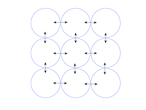
Figure 6. The 9-disc example. The 12 close-to-touching disc interactions are indicated by double arrows. For each such interaction, an additional series term in powers of $\zeta_{j}$ is included in the representation (94) for $w(z)$.

Table 6 shows our results as a function of disc separation $\epsilon$. We truncated the infinite sums at ${\mathcal{N}}$ modes and took $2{\mathcal{N}}+10$ collocation points on each circle in order to yield an over-determined linear system. Note that it is a simple matter to establish an expression for the required dipole moment from the representation (94).

As a comparison of performance, Figure 7 shows a graph of the logarithm of the disc separation against the number of modes needed to attain the correct dipole moment correct to ${\mathcal{O}}(10^{-4})$. Results are shown both for the new method given here as well as that of Cheng & Greengard [4]. The key feature is that both graphs are close to linear (albeit with different slopes). This means that both methods require just a linear increase in the degree of truncation as the order of magnitude of the separation is decreased. This is a major improvement on previous methods (e.g., the original Fourier-Laurent method) where the required number of modes appears to increase by an order of magnitude as the separation decreases by an order of magnitude and, therefore, rapidly become unviable for very small separations.

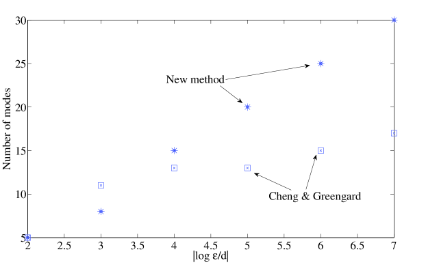
Figure 7. Graph showing the number of modes needed (for accuracy ${\mathcal{O}}(10^{-4})$ in the 9-disc example) against the logarithm of the disc separation $\log_{10}(\epsilon)$. Both methods require only a linear increase in the number of modes as the separation decreases by an order of magnitude.

9. Discussion

A new “hybrid basis scheme” has been presented to compute analytic functions exterior to a collection of close-to-touching discs and satisfying certain boundary conditions of the boundaries of those discs. The method is conceptually simple and it is easy to implement. It affords similar advantages to the method of Cheng & Greengard [4] in that it requires just a linear increase in the truncation as the disc separation decreases by an order of magnitude. The new method, however, has the advantage of not requiring analytical knowledge of any “reflection operators” to produce the coefficients of multipole expansions about higher generations of reflections. This will be important for problems involving the computation of functions analytic outside a collection of close-to-touching discs when the boundary value problems determining these functions are such that analogous reflection operators are not known analytically. It should also be clear that close-to-touching discs having unequal radii are also amenable to the same method.

One motivation for seeking a simple and effective numerical scheme for this problem is our desire to optimize a numerical scheme presented in [7] for the computation of a special transcendental function known as the Schottky-Klein prime function [1]. This function is very useful [10, 11, 12] for finding analytical solutions to problems involving multiply connected domains (indeed the function $P(\zeta,\rho)$ used to find the exact solution (14) is closely related to a special case of a Schottky-Klein prime function). This function is defined in a multiply connected circular region – one whose boundaries consist purely of circles – and, in certain applications, those circles draw close together. The hybrid basis scheme is expected to provide a viable means of accurately computing the Schottky-Klein prime function in such cases. Work on this is currently in progress.

Acknowledgments: DGC acknowledges support from an EPSRC Established Career Fellowship. ST acknowledges support from an EPSRC Platform Grant held at Imperial College London and support from the NSF DMS-110894. DGC acknowledges many useful discussions with J. S. Marshall.

10. Appendix: Alternative Representation of $K(\zeta)$

Unfortunately (21) is not in a suitable form to study its asymptotics as $\rho\rightarrow 1^{-}$. To find an alternative form it is useful to choose

(95) $$\xi=\frac{1}{\pi}\log\zeta.$$

Then it is clear from the representation (21) that

(96) $$Q(\xi)=\frac{1}{\pi}\frac{d}{d\xi}K\left(e^{\pi\xi}\right)=\frac{\zeta(\xi)}{\pi}K^{\prime}(\zeta(\xi))$$

is a doubly periodic function with periods periods $2{\rm i}$ and $2T$, where $T=(1/\pi)\log\rho^{-1}$, with double pole at $\xi=0$ and all points congruent to it, i.e., at the set of points $2{\rm i}m+2nT$ for $(m,n)\in\mathbb{Z}^{2}$. Further, from (21) it follows that

(97) $$\lim_{\xi\rightarrow 0}\xi^{2}Q(\xi)=\frac{1}{\pi^{2}}\lim_{\zeta\rightarrow 1}\left(\log\zeta\right)^{2}\zeta K^{\prime}(\zeta)=-\frac{1}{\pi^{2}}.$$

On applying Liouville’s theorem we deduce

(98) $$Q(\xi)=C_{0}-\frac{1}{\pi^{2}}\wp\left(\xi;T,{\rm i}\right)\ ,$$

for some constant $C_{0}$ that will be determined shortly, and where we have introduced the Weierstrass $\wp$ function represented by

(99) $$\wp(\xi;\omega_{1},\omega_{2})=\frac{1}{\xi^{2}}+\sum_{(m,n)\in\mathbb{Z}^{2}\setminus\{(0,0)\}}\left[\frac{1}{(\xi-2n\omega_{1}-2m\omega_{2})^{2}}-\frac{1}{(2n\omega_{1}+2m\omega_{2})^{2}}\right].$$

This representation is absolutely convergent for any $\xi$ different from $0$ and points congruent to it, and so the order of summation in $m$ and $n$ is irrelevant. To sum first in $m$, it is convenient to introduce

(100) $$\xi_{n}=\xi-2nT~{}~{}\ ,~{}~{}\xi_{0,n}=-2nT.$$

It follows that

(101) $$\wp(\xi;T,{\rm i})=\sum_{n\in\mathbb{Z}}\sum_{m=1}^{\infty}\left[\frac{1}{(\xi_{n}-2{\rm i}m)^{2}}-\frac{1}{(\xi_{0,n}-2{\rm i}m)^{2}}+\frac{1}{(\xi_{n}+2{\rm i}m)^{2}}-\frac{1}{(\xi_{0,n}+2{\rm i}m)^{2}}\right]\\ +\frac{1}{\xi^{2}}+\sum_{n\neq 0}\left(\frac{1}{\xi_{n}^{2}}-\frac{1}{4n^{2}T^{2}}\right)$$

On use of the meromorphic representation of $1/{\sinh^{2}({\pi\xi/2})}$, it follows that

(102) $$\wp(\xi;T,{\rm i})=\frac{\pi^{2}}{4\sinh^{2}\frac{\pi\xi}{2}}+\frac{\pi^{2}}{12}+\sum_{n\neq 0}\left(\frac{\pi^{2}}{4\sinh^{2}\frac{\pi\xi_{n}}{2}}-\frac{\pi^{2}}{4\sinh^{2}(\pi nT)}\right)\ ,$$

which implies

(103) $$Q(\xi)=-\frac{1}{4\sinh^{2}\frac{\pi\xi}{2}}-\frac{1}{12}-\sum_{n\neq 0}\left(\frac{1}{4\sinh^{2}\frac{\pi\xi_{n}}{2}}-\frac{1}{4\sinh^{2}(\pi nT)}\right)+C_{0}\ ,$$

where $C_{0}$ will shortly be determined. From (21) and (96), it follows that $K(e^{\pi\xi})$ from $Q(\xi)$ may be related through the following integration:

(104) $$\begin{split}K\left(e^{\pi\xi}\right)=\frac{1}{2}\coth\frac{\pi\xi}{2}&+\sum_{n\neq 0}\left\{\frac{1}{2}\coth\left(\frac{\pi}{2}(\xi-2nT)\right)+\frac{\pi\xi}{4\sinh^{2}(n\pi T)}\right\}\\ &+\left(C_{0}-\frac{1}{12}\right)\pi\xi+c.\end{split}$$

Using

(105) $$\coth z=\frac{e^{2z}+1}{e^{2z}-1}=\frac{2e^{2z}}{e^{2z}-1}-1$$

it follows that an alternative representation is

(106) $$K\left(e^{\pi\xi}\right)=\frac{e^{\pi\xi}}{e^{\pi\xi}-1}+\sum_{n=1}^{\infty}\left\{\frac{e^{\pi\xi}e^{-2nT\pi}}{e^{\pi\xi}e^{-2nT\pi}-1}+\frac{e^{-\pi\xi}e^{-2nT\pi}}{1-e^{-\pi\xi}e^{-2nT\pi}}\right\}\\ +\left(c-\frac{1}{2}\right)+\left(\sum_{n\neq 0}\frac{1}{4\sinh^{2}(n\pi T)}+C_{0}-\frac{1}{12}\right)\pi\xi$$

This reproduces the representation (21) provided,

(107) $$c=\frac{1}{2}~{}~{}\ ,~{}~{}C_{0}=\frac{1}{12}-\sum_{n\neq 0}\frac{1}{4\sinh^{2}(n\pi T)}$$

Thus, with the determination of $C_{0}$, the connection between $Q(\xi)$ and the Weierstrass $\wp$ function has been made, and with the integration constant $c$ as determined, it follows that

(108) $$\frac{1}{\pi}K\left(e^{\pi\xi}\right)=+\frac{1}{\pi^{2}\xi}+\frac{1}{2}+\int_{0}^{\xi}\left(Q(\xi^{\prime})+\frac{1}{\pi^{2}{\xi^{\prime}}^{2}}\right)d\xi\ ,$$

and hence $K$ can be determined in terms of the Weierstrass $\wp$ function through an integration. To find the uniform asymptotics for small $T$, it is better to sum over $n$ first in the meromorphic representation (101) for $\wp$. Then, using the meromorphic representation of ${\rm cosec}^{2}$, it follows that

(109) $$\wp(\xi;T,{\rm i})=\frac{\pi^{2}}{4T^{2}\sin^{2}\frac{\pi\xi}{2T}}-\frac{\pi^{2}}{12T^{2}}+\sum_{m\neq 0}\left\{\frac{\pi^{2}}{4T^{2}\sin^{2}\frac{\pi(\xi-2{\rm i}m)}{2T}}+\frac{\pi^{2}}{4T^{2}\sinh^{2}\frac{\pi m}{T}}\right\}$$

On using the relation between $K$, $Q$ and $\wp$, we find

(110) $$K\left(e^{\pi\xi}\right)=\frac{1}{2T}\cot\frac{\pi\xi}{2T}+\frac{1}{2T}\sum_{m\neq 0}\left\{\cot\left(\frac{\pi(\xi-2{\rm i}m)}{2T}\right)-\cot\left(\frac{-{\rm i}m\pi}{T}\right)\right\}\\ +\frac{1}{2}+\left(\frac{1}{2\pi T}+C_{1}\right)\pi\xi\ ,$$

where

(111) $$C_{1}=\frac{1}{12}-\frac{1}{2}\sum_{n=1}^{\infty}\frac{1}{\sinh^{2}(n\pi T)}+\frac{1}{12T^{2}}-\frac{1}{2T^{2}}\sum_{m=1}^{\infty}\frac{1}{\sinh^{2}\frac{m\pi}{T}}-\frac{1}{2\pi T}$$

$C_{1}=0$ as it must in order that $K(e^{\pi(\xi+2T)})=1+K(e^{\pi\xi})$. This follows indirectly since (21) implies that property and representation (110) has been derived in a series of steps from (21).

It is interesting to note that independently we may arrive at the same conclusion by $C_{1}$ as meromorphic function of $T$ where the residues vanish at all possible poles and the asymptotics as $T\rightarrow 0$ gives zero, implying from Liouville’s theorem that $C_{1}=0$. The single valuedness of $K$ as a function of $\zeta$ is obvious in (21). To directly check this property, i.e. that $K\left(e^{\pi(\xi+2{\rm i})}\right)=K\left(e^{\pi\xi}\right)$, is not so obvious in (110) since there is a linear term $\xi=(1/\pi)\log\zeta$. Nonetheless, this is true, as we now argue. It is useful to introduce notation

(112) $$\chi=e^{i\pi\xi/T}~{}~{}\ ,~{}~{}~{}\mu=e^{-2\pi/T}$$

Then using the exponential representation of $\cot$ function, (110) implies that

(113) $$K\left(e^{\pi\xi}\right)=\frac{\xi}{2T}+\left(\frac{1}{2}-\frac{{\rm i}}{2T}\right)+\frac{{\rm i}}{T}\left(\frac{\chi}{\chi-1}\right)+\frac{{\rm i}}{T}\sum_{m=1}^{\infty}\left(\frac{\mu^{m}\chi^{-1}}{1-\mu^{m}\chi^{-1}}-\frac{\mu^{m}\chi}{1-\mu^{m}\chi}\right).$$

We notice that the transformation $\xi\mapsto\xi+2{\rm i}$ implies that $\chi\mapsto\mu\chi$ and it is then readily checked by shifting the summation index that $K\left(e^{\pi(\xi+2{\rm i})}\right)=K\left(e^{\pi\xi}\right)$, as it must to be consistent with the single valuedness of $K(\zeta)$ in the representation (21).

References

- [1] H. Baker, Abelian functions and the allied theory of theta functions, Cambridge University Press, (1995).
- [2] C. Bender & S.A. Orszag, Advanced Mathematical Methods for Scientists and Engineers: asymptotic methods and perturbation theory, Springer, New York, (1999).
- [3] W. Burnside, On functions determined from their discontinuities and a certain form of boundary condition, Proc. Math. Soc. Lond., 22, 346–358, (1891).
- [4] H. Cheng & L. Greengard, A method of images for the evaluation of electrostatic fields in systems of closely spaced conducting cylinders, SIAM J. Appl. Math., 58(1) 122–141, (1998).
- [5] H. Cheng & L. Greengard, On the numerical evaluation of electrostatic fields in dense random dispersions of cylinders, J. Comput. Phys., 136, 629–639, (1997).
- [6] D.G. Crowdy Analytical solutions for uniform potential flow past multiple cylinders, Eur. J. Mech. B/Fluids ,25(4), 459-470, (2006).
- [7] D.G. Crowdy & J.S. Marshall, Computing the Schottky-Klein prime function on the Schottky double of planar domains, Comput. Methods Funct. Theory, 7(1), 293–308, (2007).
- [8] D.G. Crowdy and J.S. Marshall Green’s functions for Laplace’s equation in multiply connected domains, IMA. J. Appl. Math, 72, 278–301, (2007).
- [9] D.G. Crowdy, The Schwarz-Christoffel mapping to bounded multiply connected polygonal domains, Proc. Roy. Soc. A., 461, 2653–2678, (2005).
- [10] D. G. Crowdy, Conformal slit maps in applied mathematics, ANZIAM J., 53(3), 171-189, (2012).
- [11] D. G. Crowdy, The Schottky-Klein prime function on the Schottky double of planar domains, Comp. Meth. Funct. Theory, 10(2), 501-517, (2010).
- [12] D. G. Crowdy, Geometric function theory: a modern view of a classical subject, Nonlinearity, 21(10), T205-T219, (2008).
- [13] L. Greengard & M. Moura, On the numerical evaluation of electrostatic fields in composite materials, Acta Numerica, Cambridge University Press, (1994).
- [14] J. Helsing, An integral equation method for electrostatics of anisotropic composites, Proc. Roy. Soc. A, 450, 343, (1995).
- [15] J. Helsing, Thin bridges in isotropic electrostatics, J. Comput. Phys., 127, 142, (1996).
- [16] R. McPhedran, Transport properties of cylinder pairs and of the square array of cylinders, Proc. Roy. Soc. A, 408, 31–43, (1986).
- [17] R. McPhedran & G. W. Milton, Transport properties of touching cylinder pairs and of the square array of touching cylinders, Proc. Roy. Soc. A, 411, 313–326, (1987).
- [18] R. McPhedran, L. Poladian & G.W. Milton, Asymptotic studies of closely spaced, highly conducting cylinders, Proc. Roy. Soc. A, 415, 185–196, (1988).
- [19] G. Milton, The Theory of Composites, Cambridge University Press, Cambridge, (2002).
- [20] Z. Nehari, Conformal mapping, McGraw-Hill, New York, (1952).
- [21] W.J. Prosnak, Computation of fluid motions in multiply connected domains, Wissenschaft + Technik, Karlsruhe: Braun, (1987).
- [22] Lord Rayleigh, On the influence of obstacles arranged in rectangular order upon the properties of the medium, Phil. Mag., 34, 481–502, (1892).