Intermittent Map Matching with the Discrete Fréchet Distance

Abstract

In this paper we focus on the map matching problem where the goal is to find a path through a planar graph such that the path through the vertices closely matches a given polygonal curve. The map matching problem is usually approached with the Fréchet distance matching the edges of the path as well. Here, we formally define the discrete map matching problem based on the discrete Fréchet distance. We then look at the complexities of some variations of the problem which allow for vertices in the graph to be unique or reused, and whether there is a bound on the length of the path or the number of vertices from the graph used in the path. We prove several of these problems to be NP-complete, and then conclude the paper with some open questions.

1 Introduction

The map matching problem arose naturally out of sophisticated GIS (Geographic Information System) software and algorithms. With the rise of excellent satellite data and the common use of GPS (Global Positioning System) in cellphones and vehicles for navigation, an important task is map routing. There are several problems dealing with map routing, but our focus will be on the reconstruction tasks. Assume that we know the road network and can treat it as a planar embedded graph, and that we also have the GPS data from a car traveling. Often, this data is not accurate and may be noisy or approximate to the exact location of the vehicle. Thus, the data may not align with the roads properly.

The standard map matching problem is trying to find the most likely route of the vehicle on the road network given a planar metric graph to represent the road network and a polygonal curve representing the GPS data. We extend this analogy for modern instances where the data may be intermittent due to coverage or power constraints. A common issue with cellphones or hand-held GPS devices is limited battery life. A feasible situation is one where a user may only power on the device when near a city or when they need something immediately (such as making a call for directions), and afterwards they turn the device back off. Similarly, in remote areas, a user may only have reception near certain towns. Thus, tracking their phone is only possible when a signal is available. In these instances our data has discrete points of the lossy data. We still have a polygonal curve, but we can not depend on all edges of the line to be accurate location data. We know the node ordering, but the edges may not represent the actual path taken. So the problem is to find the most probable simple path of a vehicle between the recorded points on the road network.

With respect to map matching, the problem of finding a path in a graph given a polygonal curve with respect to the Fréchet distance was first posed by Alt et al. [2] as follows: Let $G=(V,E)$ be an undirected connected planar graph with a given straight-line embedding in $\mathbb{R}^{2}$ and a polygonal line $P$. Find a path $\pi$ in $G$ which minimizes the Fréchet distance between $P$ and $\pi$. They give an efficient algorithm which runs in $\mathcal{O}(pq\log q)$ time and $\mathcal{O}(pq)$ space where $p$ is the number of line segments of $P$ and $q$ is the complexity of $G$. Their version allows for vertices and edges to be visited multiple times, and is similar to the discrete version we cover in Section 4.

The recent work by Maheshwari et al. improved the running time for the map matching problem for complete graphs [15]. The original algorithm would decide it in $\mathcal{O}(pk^{2}\log k)$ where $k$ is the number of vertices in the graph, and their new algorithm solves it in $\mathcal{O}(pk^{2})$. We refer to this as the set-chain matching problem as in [21].

Map matching is an active area of research with many approaches. The two main methodologies are those based on geometric methods and ones based on Global Weight Optimization. However, the methodologies can also be classified based on the problem definition where we have local/incremental methods, global methods, and statistical methods. These can all be extended to include topological and geological conditions, current weather and traffic conditions, speed limits, and other variables that can produce more optimal routes [14, 18]. However, the work presented here is fully based on global geometric methods. We assume that we have all of the data and want to use a geometric method (the discrete Fréchet distance) to find the best fit for the input.

There has been recent work which allowed for better performance with certain types of curves, with dual simplification for an approximate result, with bounded simplification of one of the chains, and in graphs with certain properties, [4, 5, 6, 8]. With map matching, for the weak Fréchet distance, the bounds have been lowered further to $\mathcal{O}(pq)$ [7], and the problems can be better defined with a smaller error bound [19].

In reality, all GPS data is discrete, and these approaches smooth the data. There are some methods optimized for low-sampling-rate data [14], but even these assume some maximum time between samples (less than five minutes). Our purpose is to analyze data where samples may be hours apart and can not be reasonably ‘smoothed’.

This paper is organized as follows. In Section 2 we cover some necessary preliminary concepts. Section 3 formally defines the problem and scope of our investigation. Then Sections 4, 5, and 6 cover the complexities of the three variations we are considering. Finally, we conclude the paper in 7 with some future research directions and open questions.

2 Preliminaries

The discrete Fréchet distance was originally defined by Eiter and Mannila [9] in 1994, and was further expanded on theoretically by Mosig et al. in 2005 [17].

Given two polygonal curves, we define the discrete Fréchet distance as follows. We use $\mathit{d}(a,b)$ to represent the euclidean distance between two points $a$ and $b$, but it could be replaced with other distance measures depending on the application.

Definition 1.

The discrete Fréchet distance, $d_{F}$, between two polygonal curves $f:[0,m]\rightarrow\mathbb{R}^{k}$ and $g:[0,n]\rightarrow\mathbb{R}^{k}$ is defined as:

$$d_{F}(f,g)=\min_{\sigma:[1:m+n]\rightarrow[0:m],\beta:[1:m+n]\rightarrow[0:n]}\max_{s\in[1:m+n]}\Bigg{\{}d\Big{(}f(\sigma(s)),\,g(\beta(s))\Big{)}\Bigg{\}}$$

where $\sigma$ and $\beta$ range over all discrete non-decreasing onto mappings of the form $\sigma:[1:m+n]\rightarrow[0:m],\beta:[1:m+n]\rightarrow[0:n]$.

The continuous Fréchet distance is typically explained as the relationship between a person and a dog connected by a leash walking along the two curves and trying to keep the leash as short as possible. However, for the discrete case, we only consider the nodes of these curves, and thus the man and dog must “hop” along the nodes. With a dynamic programming solution for finding the discrete Fréchet distance between two polygonal curves, Eiter and Mannila proved:

Since the moves taken along the chains are discrete, finding the best walk between the two chains is relatively straightforward. By giving a dynamic programming solution for finding the discrete Fréchet distance between two polygonal curves, in [9] Eiter and Mannila proved that it could be easily solved in $\mathcal{O}(mn)$ time. Recently, Agarwal et al. provided the first subquadratic algorithm for the discrete Fréchet distance giving the following theorem.

Theorem 1.

The discrete Fréchet distance between two polygonal curves, with $m$ and $n$ vertices respectively, can be computed in $\mathcal{O}(\frac{mn\log\log n}{\log n})$ time [1].

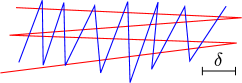
Figure 1: Figures (a) and (b) show the relationship between the discrete and continuous Fréchet distance where $o$ is the continuous and the dotted line represents the discrete distance. (a) the curves have fewer nodes and a larger discrete Fréchet distance, while (b) is the same paths with more nodes, and thus provides a better approximation of the Fréchet distance. (c) Two polygonal curves that highlight the difference between the Fréchet distance and the Hausdorff distance. Here $d_{H}\leq\delta$, but $d_{F}>2\delta$.

Figure 1 shows the relationship between the discrete and continuous Fréchet distances. In Figure 1, we have two polygonal curves (or chains) $\langle a_{1},a_{2},a_{3}\rangle$ and $\langle b_{1},b_{2}\rangle$, the continuous Fréchet distance between the two is the distance from $a_{2}$ to segment $\overline{b_{1}b_{2}}$, i.e., $\mathit{d}(a_{2},o)$. The discrete Fréchet distance is $\mathit{d}(a_{2},b_{2})$. The discrete Fréchet distance could be quite larger than the continuous distance. However, with enough evenly sample points on the two curves, the resulting discrete Fréchet distance, i.e., $\mathit{d}(a_{2},b)$ in Figure 1, closely approximates $\mathit{d}(a_{2},o)$.

The Hausdorff distance was first defined by Felix Hausdorff in 1914 [11]. Since its introduction, the Hausdorff distance has become one of the most widely used similarity measures across many disciplines.

Definition 2.

Let $X$ and $Y$ be two non-empty subsets of a metric space $(M,d)$ where $M$ is the space and $d$ the distance measure. We define their Hausdorff distance $d_{H}(X,Y)$ by

$$d_{H}(X,Y)=\max\{\sup_{x\in X}\inf_{y\in Y}d(x,y),\sup_{y\in Y}\inf_{x\in X}\mathit{d}(x,y)\},$$

where $\sup$ represents the supremum and $\inf$ the infimum.

Figure 1 shows a classic example used to demonstrate this difference. There are two polygonal curves which intersect repeatedly. Due to this crossing the Hausdorff distance is less than or equal to $\delta$, however, because the curves zigzag in different directions the Fréchet distance is greater than $2\delta$ [3].

Recently, we worked on some similar variations for the discrete set-chain matching problem. The difference is that the objective of set-chain matching is to find a path through a set of points rather than a graph. We reduce from one of these problems so we briefly give the definition and the results.

Definition 3 (The Discrete Set-Chain Matching Problem).

Instance: Given a point set $S$, a polygonal curve $P$ in $\mathbb{R}^{d}$ $(d\geq 2)$, an integer $K\in\mathbb{Z}^{+}$, and an $\varepsilon>0$.
Problem: Does there exist a polygonal curve $Q$ with vertices chosen from $S^{\prime}$ where $S^{\prime}\subseteq S$, such that $T\leq K$ and $d_{F}(P,Q)\leq\varepsilon$?

$T$ is defined in two ways. When limiting the number of nodes in the curve, $T=|Q|$, and if restricting the number of points used then $T=|S^{\prime}|$. They vary whether there is a uniqueness constraint on $s\in S$ being used as a node in $Q$ (if points may be used more than once), and whether our goal is to limit the size of the curve $Q$ or the set $S^{\prime}$. We distinguish the problems as Unique/Non-unique(U/N) Set-Chain(S) Matching(M) with a $K$ Subset/Curve(S/C). The variants are thus NSMS, NSMC, and USM.

Theorem 2.

The discrete non-unique set-chain matching problem where $T=|Q|$ is polynomial, i.e., NSMC $\in$ P [21].

Theorem 3.

The discrete non-unique set-chain matching (NSMS) problem where $T=|S^{\prime}|$ is NP-complete [21].

Theorem 4.

The discrete unique set-chain matching (USM) problem is NP-complete [21].

3 Discrete Map Matching

The definition of discrete map matching is similar to the set-chain matching definition in [21], and has three variants that we will consider.

Definition 4 (The Discrete Map Matching Problem).

Instance: Given a simple connected planar graph $G=(V,E)$ embedded in $\mathbb{R}^{2}$, a polygonal curve $P$ in $\mathbb{R}^{d}$ $(d\geq 2)$, an integer $K\in\mathbb{Z}^{+}$, and an $\varepsilon>0$.
Problem: Does there exist a path $Q$ in $G$ with the polygonal curve using vertices chosen from $V^{\prime}$ where $V^{\prime}\subseteq V$, such that $T\leq K$ and $d_{F}(P,Q)\leq\varepsilon$?

$T$ is defined in two ways. When we are minimizing the size of the chain, $T=|Q|$. If we are minimizing the vertices in the graph used then $T=|V^{\prime}|$. We look at the analogous versions of the set-chain matching problems for each of these: NMMC and NMMS. We then consider the version where the vertices in the path must be unique and only used once, which we label UMM. Note that when the vertices are unique the two minimization problems ($|Q|$,$|V^{\prime}|$) are equivalent. For reference, the naming convention is Unique/Non-unique(U/N) Map(M) Matching(M) with a $K$ Subset/Chain(S/C).

4 Map Matching with $T=|Q|$ (NMMC)

When focused solely on the length of $Q$, the problem is similar to the set-chain version (NSMC) [21]. The problem has an almost identical optimal substructure, so we forgo the proof here. The recurrence to find the minimum size of $Q$ (in number of vertices) is given in Equation 1. The actual dynamic programming algorithm is also omitted, but is straightforward. The recurrence uses a 2D array $M$ of size $|V|\times|P|$ where the first row and column are initialized to one if $\mathit{d}(v_{1},p_{k})\leq\varepsilon$ where $1\leq k\leq|P|$ and $\mathit{d}(v_{k},p_{1})\leq\varepsilon$ where $1\leq k\leq|V|$. The values are set to $K+1$ otherwise. This is polynomial with the worst case being in a complete graph, which is equivalent to the discrete set-chain matching version. If the graph is not complete, the complexity will be lower since each vertex $v$ only looks at its neighbor set, $N(v)$.

$$M[i,j]=\min\begin{cases}M[i,j\mbox{-}1],&\mbox{if }\mathit{d}(v_{i},p_{j})\leq\varepsilon,v_{i}\in N(v_{i\mbox{-}1}),M[i,j\mbox{-}1]\neq K\mbox{+}1\\ \underset{k\in N(v_{i})}{\min}M[k,j\mbox{-}1]+1,&\mbox{if }\mathit{d}(v_{i},p_{j})\leq\varepsilon,v_{i}\in N(v_{i\mbox{-}1}),M[i,j\mbox{-}1]=K\mbox{+}1\\ K+1,&\mbox{if }\mathit{d}(v_{i},p_{j})>\varepsilon\mbox{ or }v_{i}\notin N(v_{i\mbox{-}1})\end{cases}$$ (1)

Theorem 5.

The discrete Non-unique Map Matching (NMMC) problem where $T=|Q|$ is in P.

Proof.

This problem is similar to NSMC ([21]) with the restriction of which vertices are viable given the previous choice. Rather than looking at all values for the last vertex, it is restricted to only those vertices which have an edge between them. Thus, the problem has a similar solution and is polynomial. $\square$ ∎

5 Map Matching with $T=|V^{\prime}|$ (NMMS)

This problem has proven more difficult to analyze than the other versions of the discrete map matching problem. With the discrete Fréchet distance we show that it is NP-complete for general graphs (Theorem 1), and we show that with planar graphs the problem is NP-complete under the Hausdorff distance (Theorem 6). Even though we show these results, we did not prove the complexity for the planar version under the discrete Fréchet distance. We believe this problem to also be NP-complete, however, we leave this problem for future work.

Corollary 1.

Discrete non-unique map matching where $T=|V^{\prime}|$ in general graphs is NP-complete.

Proof.

By a simple reduction from NSMS (Theorem 3) we show this is true. Given a set of points $S$, a polygonal curve $P$, $\varepsilon>0$, and a $K\in\mathbb{Z}^{+}$, we build a complete graph $G=\{V,E\}$ with the vertices being the points in $S$, i.e. $V=S$ and the number of edges $|E|={|S|\choose 2}$.

This embedding allows all possible paths to be explored for $Q$, and the path it returns will be the same for both NMMS and NSMS. Thus, there exists a polygonal curve $Q$ with nodes taken from $S^{\prime}\subset S$, such that $|S^{\prime}|\leq K$ and $d_{F}(P,Q)\leq\varepsilon$ if and only if there exists a path $Q^{\prime}$ in $G$ such that the vertices in $Q^{\prime}$ are taken from $V^{\prime}\subset V$, such that $|V^{\prime}|\leq K$ and $d_{F}(P,Q^{\prime})\leq\varepsilon$. $\square$ ∎

Theorem 6.

Discrete non-unique map matching with $T=|V^{\prime}|$ in planar graphs under the Hausdorff distance is NP-complete.

Proof.

This is a straight-forward reduction from the Hamiltonian circuit problem in grid graphs [12]. Let $G_{k}$ be a grid graph with $k$ vertices such that any vertex $v\in G_{k}$ is located at $v_{x},v_{y}\in\mathbb{Z}^{+}$ and $G_{k}$ is an induced subgraph of the infinite unit grid graph $G_{\infty}$. For our construction we let $G=G_{k}$ and we let $P$ be the vertices $V$ of $G$ ordered in any way as a polygonal chain.

There exists a Hamiltonian circuit in $G_{k}$ if and only if there exists a path $Q$ in $G$ such that $|Q|=|V|$ and $d_{H}(P,Q)=0$.

If there is a Hamiltonian circuit $Q^{\prime}$ on the graph, then by definition, this path (with the start/end vertex arbitrarily chosen) has $d_{H}(G,Q^{\prime})=0$ since it covers every edge and vertex. Also, since $|Q^{\prime}|=|V|$, $|Q|=|V|$.

Given a path $Q$ in $G=G_{k}$ where $|Q|=|V|$ and $d_{H}(P,Q)=0$. Note that this path must visit every edge and vertex since $d_{H}(P,Q)=0$. If $|Q|=|V|$, it must only visit each vertex once, and thus the path must be a Hamiltonian circuit. $\square$ ∎

6 Unique Map Matching (UMM)

Map matching with unique vertices is an interesting and relevant problem. In most applications related to map matching where the graph is planar, rarely would a vertex be visited multiple times. In the GPS application of a vehicle on a road network, this would be equivalent to a car visiting the same intersection multiple times. This may occur, but when trying to find the likely path of a vehicle from the origin to the destination we can disregard self-intersecting data as unimportant overall.

We address discrete unique map matching where any vertex in the graph can be used at most once in the path, and show that this problem is NP-complete via a reduction from planar 3-SAT [13]. Planar 3-SAT is a 3-SAT formula that can be drawn as a planar graph with vertices representing clauses and variables, and the edges representing inclusion of a variable in a clause. This is a convenient form of 3-SAT for geometric reductions since a crossover gadget is unnecessary.

By standard convention, we first introduce several planar “gadgets” that we then arrange in our reduction. We will build up the gadgets in a piecewise manner, and then show how they are connected to form a single polygonal curve and a planar graph. Due to the length of this section, we cover the gadgets and then formally do the reduction with the assumption of their correctness.

Let $\varphi$ be the 3-SAT formula represented by the input instance of planar 3-SAT with $N$ variables and $M$ clauses. Given an $\varepsilon>0$, we construct a planar graph $G$ and a polygonal curve $P$. We show that $\varphi$ is satisfiable if and only if with our construction there exists a path $Q$ with unique nodes from the vertices in $G$ such that $d_{F}(P,Q)\leq\varepsilon$.

6.1 The Chain Gadget

In order to retain a true or false selection, we first show a ‘chain’ gadget used to transfer information from the variables to the clauses. Figures 2(a) and 2(b) show a polygonal curve with a ladder graph structure that constitute a chain with true and false paths shown, respectively. Since the nodes used in $G$ may only be used once, a path through this graph that maintains $d_{F}(P,Q)\leq\varepsilon$ only has two possibilities. Starting at the top left vertex a path going down is a true setting and going to the right is false.

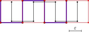
(a) True Chain

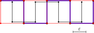
(b) False Chain

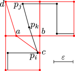
(c) Elbow

Figure 2: (a) A chain with a true path. (b) A chain with a false path. (c) An elbow in order for the chain to make turns.

Figure 2(c) shows how the chain can make a right angled turn while maintaining the true or false path. This allows the chains to be configured in a natural way with a clean layout. Note the extra edges of the graph ($e_{ac}$ and $e_{ad}$) in the corner which allows the true path to go around the vertex $b$. Since a false path must pass through $a$ and $b$ to cover $p_{i}$ and then $p_{k}$, it must continue up from $b$ in order to cover $p_{j}$. The true path goes through $c$ and has already covered $p_{i}$ so it can then go through $a$ via $e_{ac}$ and cover $p_{k}$, and then via $e_{ad}$ it goes around the outside of the corner to cover $p_{j}$ and then comes down to $b$.

6.2 The Variable Gadget

A chain is the basis of the variable gadget, but we also attach an additional diamond structure along with another polygonal curve for the diamond graph components. Figure 3 shows the planar graph and the two pieces of $P$ necessary for each variable gadget. The additional diamond shapes are needed in order to force the alternation between true and false states.

Setting a variable true or false works identically to the chain gadgets. For a variable $x_{i}$, to set the variable true, the path begins at $c_{i_{1}}$ and visits vertex $d_{i_{1}}$ next (Figure 3(a)), and to set $x_{i}$ false, the path begins at $c_{i_{1}}$ and goes through vertex $v_{i_{1}}$ and $c_{i_{2}}$. The chains will connect onto the $a_{i}$ nodes with odd subscripts being $x_{i}$ ($a_{i_{1}},a_{i_{3}},\dots$), and even subscripts representing connections for $\lnot x_{i}$ ($a_{i_{2}},a_{i_{4}},\dots$). The $a_{i}$ vertices connect by being shared on one edge of a chain as shown in the example of Figure 5. Thus, a true path in the variable does not use the $a_{i}$ vertex where the chain attaches and the chain can use that edge (for a true path), but a false variable path does require the vertex $a_{i}$ which means the chain will not be able to use the edge that attaches and will also have a false path setting. We also note that the nodes $p^{\prime}_{i_{3}}$, $p^{\prime}_{i_{6}}$, $p^{\prime}_{i_{9}}$, etc. are within $\varepsilon$ of only the $a_{i}$ and $v_{i}$ vertices.

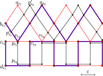
(a) True Variable Gadget

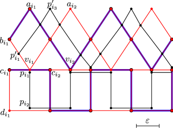
(b) False Variable Gadget

Figure 3: Variable gadgets with path settings for (a) true (b) false. A path begins at $c_{i_{1}}$ and passes through $d_{i_{1}}$ for true and through $v_{i_{1}}$ and $c_{i_{2}}$ for false.

6.3 The Clause Gadget

For the clause gadget, we assume that three ‘chains’ are attached to variable gadgets and then meet at the junction shown in Figure 4. The clause gadget is planar, but our path along the edges of the graph will no longer be a polygonal curve. The discrete Fréchet distance is valid since the distances are based on the nodes and not the edges of the curve, but this would drastically alter the continuous Fréchet distance.

The vertices in the center are important since many of the edges curve (or turn) in the space without a vertex. This is necessary for our reduction, and thus is true for distance in the space, but does not hold for the discrete Fréchet distance based on network distance [10]. We can attach chains at one vertex to the top vertex in the variable gadgets. These chains then lead to the clause gadget. See Figure 5 for an example.

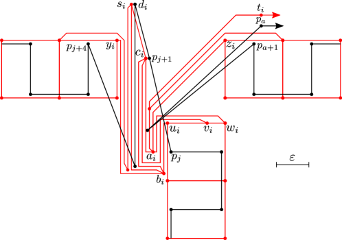
Figure 4: A clause gadget with three chains meeting.

At a high level, if a path is true in the chain it will not need to use the last edge. We will refer to the three variables in our clause as $x_{l}$, $x_{c}$, and $x_{r}$ for left, center, and right, respectively. For $x_{l}$, if the path is true, then it can use the edge to $s_{i}$. If the path is false it will end at $y_{i}$ and there is only one possible edge. Similarly, if $x_{r}$ is true, it uses the edge to go to $t_{i}$, but a false path ends at $z_{i}$. In understanding the clause gadget of clause $C_{i}$, we need focus on the two vertices $a_{i}$ and $b_{i}$. These two act as the Boolean ‘or’ operators which allow only two of the variables to be false, and thus requiring at least one to be true. Since vertices can only be used once in a path, each one (of $a_{i}$ and $b_{i}$) allow only one edge coming from a variable to be used.

When $x_{l}$ is false, the path ending at $y_{i}$, it must follow onto $b_{i}$ and then go to $s_{i}$. Similarly, if $x_{r}$ has a false path ending at $z_{i}$, it must follow onto $a_{i}$ and then go to $t_{i}$. Notice that $a_{i}$ and $b_{i}$ are within $\varepsilon$ of $p_{j}$. If $x_{c}$ has a false path, then it can go from $w_{i}$ to $a_{i}$ or go to $u_{i}$ and then $b_{i}$. This means that if it is false, it can go to either of the center vertices attached to $x_{l}$ ($b_{i}$) or $x_{r}$ ($a_{i}$). Thus, only two of them can be false. If $x_{c}$ is true, it still needs an edge to get to $c_{i}$ without crossing the edges attached to $a_{i}$ and $b_{i}$. If $x_{c}$ is true, then a path can go through $u_{i}$ and then through $v_{i}$ to $c_{i}$. Thus, our clause works as a Boolean ‘or’ of the three variables where at least one variable must be true.

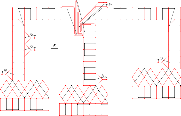
Figure 5: Example UMM clause with three variables $c_{i}=(\lnot x_{1}\lor x_{2}\lor\lnot x_{3})$ with assignments $x_{1}=0,$ $x_{2}=0,$ $x_{3}=1$.

6.4 Connecting the Gadgets

Now we discuss how everything is connected so that $G$ is planar and connected, and that $P$ is a single continuous polygonal curve. Referring to our clause, $c_{i}$ and $s_{i}$ meet via $d_{i}$ which allows a path to connect the two variables without changing their path settings. Looking at our example (Figure 5) we see that this leaves six polygonal curve endings (or three segments) in the clause gadget and connecting chains. The two exiting nodes ($p_{i},p_{j}$) from $x_{c}$ and $x_{r}$ can simply be connected (or attached to the outside of another nested clause). Similarly, $p_{y}$ and $p_{z}$ can simply be connected if there are no nested clauses under the left leg. This now means each clause uses a single polygonal curve and has two nodes ($p_{a},p_{b}$) to attach to other clauses or the variables along with the associated graph edges.

We can see in the example clause in Figure 5 that the graph and polygonal curve leave on the outside of the clause. By design, the middle and right leg connect on the interior. Thus, in a planar 3-SAT instance, if there is a nested clause, these lines ($p_{i},p_{j}$) connect to the outside of the nested clause. Similarly, the points ($p_{y},p_{z}$) connect to the outside of any clause under the left side. In both cases, if there is no other clause, the pair of points connect to each other. If there are multiple clauses under one side, then they are chained together, i.e., $p_{a}$ from one clause connects to $p_{b}$ from the other.

For some planar 3-SAT instances, it is necessary to attach chains above and below the variable gadget. We can attach another diamond structure on the other side of our variable gadget and have clauses on both sides of the variables. The only difference is that it begins with $\lnot x$ in the alternating connections.

We can then define a simple process to connect them. When saying we are connecting we mean to put an edge between the two nodes of the polygonal curves and to put an edge between the vertices of the graph. We only refer to one of the connections for simplicity. The order the polygonal chain segments are connected is unimportant as long as the two ends are not within $\varepsilon$ of each other, and the two graph components can be connected without intersection.

First, connect the variables together. Attach the ending vertex and polygonal node to the start of the next variable. Connect the chain sections and then the diamond structures. Following, connect the last variable to the closest outside clause variable ($p_{a}$). The clauses are then chained together by outside vertices and the nested clauses link to the inside edges. As mentioned, if there are no nested clauses, then connect the pairs ($p_{i},p_{j}$) and ($p_{y},p_{z}$).

6.5 The Reduction

Theorem 7.

The discrete unique map matching (UMM) problem is NP-complete for planar graphs.

Proof.

Given a planar 3-SAT instance $G_{\varphi}=\{V,E\}$ with vertices $V=X\cup C$ such that the vertices represent variables $X=\{x_{1},x_{2},\dots,x_{N}\}$ and clauses $C=\{C_{1},C_{2},...,C_{M}\}$, and the edges $E=\{e_{1},e_{2},\dots,e_{Z}\}$ connect variables to clauses with the degree of each $C_{i}\in C$ being three. Given the planar 3-SAT instance $G_{\varphi}$, we construct a polygonal curve $P$ and a planar graph $H$ using an $\varepsilon>0$ based on the method described. This construction takes $\mathcal{O}(|C|+|X|+|E|)$ and is polynomial. The sizes of $P$ and $H$ are dependent on $\varepsilon$ and the metric space. In general, for any edge $e_{i}\in E$ in the space, where $\lVert e_{i}\rVert$ is the length of the edge, there are $\lceil 2\lVert e_{i}\rVert/\varepsilon\rceil$ vertices and edges in $H$, and nodes of $P$ used to transfer information along that edge.

The planar 3-SAT formula $\varphi$ is satisfiable if and only if there exists a path $Q$ with nodes from the vertices in $H$ such that $d_{F}(P,Q)\leq\varepsilon$ and each vertex represents a unique node in $Q$.

Given $\varphi$ is satisfiable, then for every clause, there is at least one variable which has a true value. In our construction this means at least one chain does not need a path through the two points ($a_{i},b_{i}$ for clause $C_{i}$), and thus we can easily find a $Q$ such that $d_{F}(P,Q)\leq\varepsilon$.

In the other direction, assume there exists a path $Q$ through $V^{\prime}\subset V$ of $H$ such that $d_{F}(P,Q)\leq\varepsilon$. There must be at least one true path in a chain at each clause, and since the three chains keep this setting back to the variable we know it had this setting at the variable. Since we also know that the variables alternate between a true and false setting, the attached chain has the correct Boolean value associated with the path. Thus, for every variable attached to a clause, it has the correct true or false path setting. Therefore, if $d_{F}(P,Q)\leq\varepsilon$, then the current setting of each variable satisfies $\varphi$.

Last, we know the problem is in NP. Given an instance $I$ we can check whether $d_{F}(P,I)\leq\varepsilon$ in $\mathcal{O}(|P||I|)$ time via Theorem 1. $\square$ ∎

Although our focus is on the discrete Fréchet distance, our reduction actually works to show that the UMM problem is still NP-complete when based on the continuous Fréchet distance. This was simultaneously and independently proven in [16], but has not been formally published. Since this result is available, we do not rigorously show that our construction works for the continuous Fréchet distance here.

7 Conclusion

In this paper we looked at discrete map matching based on the discrete Fréchet distance for the first time, and further defined some variations based on restricting the problem to unique nodes, the number of nodes allowed in the curve, or the number of vertices to choose from. We proved that the unique nodes version is NP-complete. If the number of vertices is restricted, we proved that the problem is NP-complete for regular graphs, and for planar graphs under the Hausdorff distance. We proved that finding any path while only limiting the length of the path is polynomial, and gave the recurrences for a dynamic programming implementation. We conclude with a few open questions.

(1) What is the complexity of NMMS based on the discrete and continuous Fréchet distance?

(2) Are there good approximation algorithms for the optimization versions?

(4) Are there any special cases that are tractable for real-world applications?

References

- [1] P. K. Agarwal, R. B. Avraham, H. Kaplan, and M. Sharir. Computing the discrete fréchet distance in subquadratic time. In Proc. of the 24th Annual ACM-SIAM Sym. on Discrete Algorithms, SODA’13, pages 156–167. SIAM, 2013.
- [2] H. Alt, A. Efrat, G. Rote, and C. Wenk. Matching planar maps. Journal of Algorithms, 49(2):262–283, Nov 2003.
- [3] H. Alt and M. Godau. Computing the Fréchet distance between two polygonal curves. Int. Journal of Computational Geometry and Applications, 5:75–91, 1995.
- [4] S. Brakatsoulas, D. Pfoser, R. Salas, and C. Wenk. On map-matching vehicle tracking data. In Proc. of the 31st Int. Conf. on Very Large Data Bases, VLDB’05, pages 853–864. VLDB Endowment, 2005.
- [5] K. Buchin, M. Buchin, and Y. Wang. Exact algorithms for partial curve matching via the Fréchet distance. In Proc. of the 20th Annual ACM-SIAM Sym. on Discrete Algorithms, SODA’09, pages 645–654, 2009.
- [6] D. Chen, A. Driemel, L. J. Guibas, A. Nguyen, and C. Wenk. Approximate map matching with respect to the Fréchet distance. In Proc. of the 13th Workshop on Algorithm Engineering and Experiments, ALENEX’11, pages 75–83. SIAM, 2011.
- [7] D. Chen, L. J. Guibas, Q. Huang, and J. Sun. A faster algorithm for matching planar maps under the weak Fréchet distance. Unpublished, December 2008.
- [8] A. Driemel, S. Har-Peled, and C. Wenk. Approximating the Fréchet distance for realistic curves in near linear time. Discrete & Comp. Geom., 48(1):94–127, 2012.
- [9] T. Eiter and H. Mannila. Computing discrete Fréchet distance. Technical Report CD-TR 94/64, Information Systems Dept., Technical University of Vienna, 1994.
- [10] C. Fan, J. Luo, and B. Zhu. Fréchet-distance on road networks. In Proc. of the 9th Int. Conf. on Comp. Geometry, Graphs and Appl., CGGA’10, pages 61–72, 2011.
- [11] F. Hausdorff. Grundzüge der mengenlehre. Von Veit, Leipzig, 1914.
- [12] A. Itai, C. H. Papadimitriou, and J. L. Szwarcfiter. Hamilton paths in grid graphs. SIAM Journal on Computing, 11(4):676–686, 1982.
- [13] D. Lichtenstein. Planar Formulae and Their Uses. SIAM Journal on Computing, 11(2):329–343, 1982.
- [14] Y. Lou, C. Zhang, Y. Zheng, X. Xie, W. Wang, and Y. Huang. Map-matching for low-sampling-rate gps trajectories. In Proc. of the 17th ACM SIGSPATIAL Int. Conf. on Advances in G.I.S., GIS’09, pages 352–361, New York, NY, 2009. ACM.
- [15] A. Maheshwari, J.-R. Sack, K. Shahbaz, and H. Zarrabi-Zadeh. Staying close to a curve. In Proc. of the 23rd Annual Canadian Conf. on Computational Geometry, CCCG’11, 2011. August 10-12, 2011.
- [16] W. Meulemans. Map matching with simplicity constraints. CoRR, abs/1306.2827, 2013.
- [17] A. Mosig and M. Clausen. Approximately matching polygonal curves with respect to the Fréchet distance. Comp. Geom.: Theory and Appl., 30(2):113–127, Feb 2005.
- [18] H. Wei, Y. Wang, G. Forman, and Y. Zhu. Map matching by Fréchet distance and global weight optimization. Technical Report SJTU_CS_TR_201302001, Department of Computer Science, Shanghai Jiao Tong University, 2013.
- [19] C. Wenk, R. Salas, and D. Pfoser. Addressing the need for map-matching speed: Localizing global curve-matching algorithms. In 18th Int. Conf. on Scientific and Statistical Database Management, SSDBM’06, pages 379–388, 2006.
- [20] T. Wylie. The Discrete Fréchet Distance with Applications. PhD thesis, Montana State University, 2013.
- [21] T. Wylie and B. Zhu. Following a curve with the discrete Fréchet distance. Theoretical Computer Science, 2014. doi:http://dx.doi.org/10.1016/j.tcs.2014.06.026.