Do debit cards increase household spending? Evidence from a semiparametric causal analysis of a survey

Abstract

Motivated by recent findings in the field of consumer science, this paper evaluates the causal effect of debit cards on household consumption using population-based data from the Italy Survey on Household Income and Wealth (SHIW). Within the Rubin Causal Model, we focus on the estimand of population average treatment effect for the treated (PATT). We consider three existing estimators, based on regression, mixed matching and regression, propensity score weighting, and propose a new doubly-robust estimator. Semiparametric specification based on power series for the potential outcomes and the propensity score is adopted. Cross-validation is used to select the order of the power series. We conduct a simulation study to compare the performance of the estimators. The key assumptions, overlap and unconfoundedness, are systematically assessed and validated in the application. Our empirical results suggest statistically significant positive effects of debit cards on the monthly household spending in Italy.

FLA

and

M1Supported in part by the U.S. National Science Foundation (NSF) under Grant DMS-11-27914 to the Statistical and Applied Mathematical Sciences Institute (SAMSI). M2Supported in part by NSF Grant SES-1155697.

1 Introduction

The past few decades have seen a steadily increasing global trend in the use of noncash payment instruments such as credit, debit, charge and prepaid cards as well as electronic money. Research on the psychology of consumer behavior provides a theoretical basis for supporting the thesis that payment instruments can play a significant role in consumer decisions. Possibly the most important concept coming out of this field of research is mental accounting, that is, the set of cognitive operations used by individuals and households to organize, evaluate, and keep track of financial activities [Thaler (1985, 1999)]. Starting from this concept, recent research has proposed theories on prospective accounting, coupling, retrospective evaluations, and financial resources accessibility [Prelec and Loewenstein (1998), Soman (2001), Morewedge, Hotzman and Epley (2007)], which have stimulated deeper investigation on the effects of noncash payment instruments on consumption. Indeed, there has been substantial evidence that consumers who have cards overspend compared to those who do not [e.g., Burman (1974), Hirschman (1979), Tokunaga (1993), Cole (1998), Mann (2006)]. However, the observed association between the level of spending and the possession of cards does not necessarily indicate the existence of causal links; the association could be due to differences between the characteristics of card owners and nonowners, or to differences in the situations in which cash and cards are the preferred methods of payment. Despite the practical importance of the problem and the large literature on causal inference in statistics and economics, to our knowledge, there is essentially no analysis on the causal effects of payment instruments on consumer spending.

The main objective of this paper is to investigate the causal effects of debit cards possession on spending, using data from the Italy Survey on Household Income and Wealth (SHIW) within the Rubin Causal Model [RCM; Rubin (1974, 1978), Holland (1986)]. Debit cards are defined as cards enabling the holder to have purchases directly charged to funds on his account at a deposit-banking institution [C.P.S.S. (2001)], and in Italy they are usually called “carte Bancomat.” Our focus on debit cards is principally motivated by the fact this payment instrument does not allow consumers to incorporate additional long-term sources of funds, as in the case of credit cards. By considering debit cards, it is therefore possible to eliminate the confounding intertemporal reallocations of wealth from the psychological effects on spending [Soman (2001)]. Alternatively, prepaid cards could be relevant to the current study’s objectives, because they do not allow the consumer to be granted a line of credit. However, their diffusion in Italy is at the moment low.

Under the RCM, each unit has a potential outcome corresponding to each treatment level, and the causal effect is defined as a comparison between the potential outcomes of a common set of units. Ideally we would conduct an analysis with units being individuals possessing debit cards, because debit cards are typically issued to individuals. However, SHIW collects information only on the household level. To mitigate this problem, in our study, we set household as the unit, but limit the sample of treated units to the households possessing one and only one debit card. Such a choice ensures that a possible effect on household spending will be due only to the individual possessing the card, which is usually the head of the household. Formally, the unit-level causal effect of holding debit card is defined as the difference between the potential spending corresponding to with one and only one debit card and without debit cards. In particular, we are interested in the “population average treatment effect for the treated” (PATT), that is, the average causal effect for the households holding one debit card. The PATT identifies the change in the average consumption for the households holding one debit card and due only to the debit card, and thus provides a scientifically sound answer to the question of whether debit cards encourage spending.

Because at most one potential outcome is observed for each unit, unit-level causal effects are generally not identifiable. Nevertheless, population average causal effects can be identified under some assumptions. The most important and widely adopted identifying assumption is unconfoundedness [Rosenbaum and Rubin (1983)], which rules out self-selection into the treatment. Another key assumption is overlap, which ensures overlap in covariate distributions between groups. We maintain both assumptions throughout the paper. An integral component of our application is to systematically assess, directly or indirectly, the plausibility of these assumptions.

We estimate the PATT from the SHIW data using three existing estimators, based on regression, propensity score weighting, mixed matching and regression, as well as a new doubly-robust (mixed weighting and regression) estimator. To flexibly model the large number of covariates, we choose to proceed from a semiparametric perspective based on power series specifications. Over the last decade, non- and semi-parametric methods have been revealed to be successful in attaining desirable properties where standard parametric models fail. In fact, under a semiparametric power series approach, the efficiency bound for a causal effect estimator under unconfoundedness [Hahn (1998)] is attained by a regression-based method [Imbens, Newey and Ridder (2005)] or by weighting on the estimated propensity scores [Hirano, Imbens and Ridder (2003)]. Other advantages include the following: first, a correction based on power series regressions allows for a matching method to be unbiased and consistent [Abadie and Imbens (2006)]; second, the overlap assumption can be easily assessed by relying on undersmoothed specification for the propensity score [Imbens (2004)]; and, finally, the assessment of unconfoundedness can be performed by testing equality restrictions on the coefficients of power series regressions for the treated and untreated units [Crump et al. (2008)]. Despite these advantages, power series-based semiparametric approaches have not been widely used in practice.

The rest of the paper is organized as follows: Section 2 presents the theories and some empirical findings, mainly from the consumer psychology literature, that motivate the current research problem. Section 3 sets up the causal approach, introduces the new doubly-robust estimator and three existing estimators, and describes the semiparametric specification. A small simulation study is carried out in Section 4 to compare the estimators. In Section 5, we first present some preliminary results of the real data, then assess the key assumptions, and finally apply the semiparametric methods to estimate the causal effects of possessing debit cards on household spending. Section 6 concludes.

2 Motivating background

Research in psychology and consumer science shows that consumers are highly sensitive to contextual information that may induce perceptual contrasts when making evaluations [Helson (1964), Hsee et al. (1999), Kahneman and Miller (1986), Morewedge, Hotzman and Epley (2007), Parducci (1995)]. This field of research provides arguments for supporting that a consumer’s evaluation of the amount of disposable financial resources can be heavily influenced by the size of the financial resources cognitively, or temporarily, accessible at the time of purchasing [Heat and Soll (1996), Soman and Cheema (2002), Thaler (1985)]. Based on results from one small experiment, Morewedge, Hotzman and Epley (2007) suggested that consumers perceive a unit of consumption to be cheaper when large, as opposed to, small financial resources are made cognitively accessible. As a result, large financial accounts, such as the money in one’s savings account, are likely to increase the likelihood of consumption as compared to small financial resources, such as the amount of money in one’s wallet. But Morewedge et al. did not explain when consumers are likely to think in terms of small versus large disposable resources. It is reasonable to postulate that the method of payment can activate thoughts about different financial resources. Therefore, it would be useful to investigate the effects of payment instruments that provide direct access to larger financial resources, such as debit or credit cards, on consumption.

A second motivation stems from the findings of Soman (2001), who showed that payment instruments influence the memory for and the impact of past expenses on spending behavior. Two features of payment mechanisms—rehearsal of the price paid and the immediacy of wealth depletion—were manipulated using a controlled experiment in which recall and retrospective evaluation of payments were measured simultaneously with the purchase intention. The experiment involved four different payment instruments: checks, debit cards, charge cards, and charge checks. Debit cards are here characterized by no rehearsal (like charge cards) in that consumers do not need to write down the total amount; rather, they involve immediate wealth depletion (like checks). Soman’s study shows that past payments significantly reduce future spending intentions when the payment instrument requires consumers to write down the amount paid as well as when the consumer’s wealth is depleted immediately rather than with a delay.

Some attempts to quantify the effects of payment instruments, especially credit cards, on spending were conducted by small-scale randomized experiments [Feinberg (1986), Prelec and Simester (2001), Soman (2001)]. All of these studies were performed on a small sample of volunteers, raising the concern of external validity, as there may be significant difference between the volunteers and the targeted population. Moreover, all but one of the experiments involve only simulated series of payments rather than real monetary transactions. Also, the experiment in Feinberg (1986) that is based on real monetary transactions only manipulates exposure to credit card stimuli, not the payment method itself.

Population-based observational studies generally do not match the internal validity of randomized experiments, but they usually offer better external validity. Therefore, a careful causal analysis on a large population-based observational data with information on real monetary transactions, which was absent in the literature to our knowledge, would provide a good complement to these randomized studies. This motivates our analysis of the SHIW data, a biennial, nationally representative survey run by Bank of Italy aiming to collect information on several aspects of Italian households’ economic and financial behavior. SHIW contains rich information related to household characteristics, spending, and payment instruments, and thus provides a great opportunity to evaluate the causal effect of debit card possession on spending in Italian households.

3 Causal inference

3.1 Setup, estimand, and assumptions

Consider a large population of units, each of which can potentially be assigned a treatment indicated by $z$, with $z=1$ for active treatment and $z=0$ for control. A random sample of $N$ units from this population is drawn to evaluate the treatment effect on some outcome. For each unit $i$ $(i=1,\ldots,N)$, let $Z_{i}$ be the observed treatment status, and $\mathbf{X}_{i}=\{X_{i1},\ldots,X_{ir}\}$ be a set of $r$ pre-treatment variables (i.e., covariates) and the $N\times r$ matrix $\mathbf{X}$ has $i$th row equal to $\mathbf{X}_{i}$. We assume the Stable Unit Treatment Value Assumption [SUTVA; Rubin (1980)], that is, no interference between the units and no different versions of a treatment. Then each unit $i$ has two potential outcomes $Y_{i}(0)$ and $Y_{i}(1)$, corresponding to the potential treatment levels $z=0$ and $z=1$, respectively. Between the two potential outcomes, only the one corresponding to the observed treatment status, $Y_{i}=Y_{i}(Z_{i})$, is observed. In our study, the unit is the household; the treatment status equals one if the household possesses one and only one debit card and zero if the household does not possess debit cards; and the outcome is the monthly household spending on all consumer goods. SUTVA is deemed reasonable in this setting, as the holding of debit cards in one household does not seem to affect the potential spending of other households.

Our primary interest lies in the causal effect of having debit card on spending for the households who possess one and only one debit card. Therefore, the target causal estimand is the population average treatment effect for the treated (PATT):

$$\tau^{\mathrm{PATT}}\equiv\mathbb{E}\bigl{\{}Y_{i}(1)-Y_{i}(0)|Z_{i}=1\bigr{\}}.$$ (1)

To identify the PATT, we maintain the standard assumption of unconfoundedness.

Assumption 1 ((Unconfoundedness)).

The treatment assignment is independent of the potential outcomes given a vector of pre-treatment covariates $\mathbf{X}_{i}$:

$$\bigl{\{}Y_{i}(0),Y_{i}(1)\bigr{\}}\perp Z_{i}|\mathbf{X}_{i}.$$

Unconfoundedness assumes that the treatment assignment is randomized conditional on a set of pre-treatment covariates, and thus rules out self-selection into the treatment. It is also referred to as the assumption of “no unmeasured confounders.” Under unconfoundedness, we have $\Pr(Y_{i}(z)|\mathbf{X}_{i})=\Pr(Y_{i}|Z_{i}=z,\mathbf{X}_{i})$, and thus causal effects can be estimated by the average difference in the observed outcome between the groups that have balanced covariate distributions. However, unconfoundedness, sometimes questionable in observational studies, is generally untestable. Nevertheless, there are indirect ways to assess its plausibility. In particular, we will adopt the proposal of Crump et al. (2008) to assess unconfoundedness by a test on a pseudo-outcome, namely, the lagged outcome in this application.

The second assumption ensures overlap in the covariate distributions between the treatment and control groups.

Assumption 2 ((Overlap)).

Each unit in the population has a nonzero probability of receiving each treatment:

$$0<e(\mathbf{x})\equiv\Pr(Z_{i}=1|\mathbf{X}_{i}=\mathbf{x})<1\qquad\forall\mathbf{x},$$

where $e(\mathbf{x})$ is called the propensity score [Rosenbaum and Rubin (1983)]. Violation to the overlap assumption generally leads to operational difficulties, such as large variances in weighting estimators, as well as conceptual difficulties because the potential outcome under one treatment level for certain values of covariates would never be observed and the causal effect would be a priori counterfactual. The overlap assumption is directly testable, for example, by visually inspecting the distributions of the estimated propensity scores between groups. The combination of Assumptions 1 and 2 is referred to as “strong ignorability” [Rosenbaum and Rubin (1983)].

When the interest is in estimating the PATT, the outcome distribution for the treated is directly estimable so that the two assumptions can be slightly weakened [Heckman, Ichimura and Todd (19978)] and replaced by unconfoundedness only for the untreated units, $Y_{i}(0)\perp Z_{i}|\mathbf{X}_{i}$, and with the weak overlap, $\Pr(Z_{i}=1|\mathbf{X}_{i}=\mathbf{x})<1$ for any $\mathbf{x}$.

3.2 Estimators

We first introduce three existing estimators for thePATT. Let $\mu_{z}(\mathbf{x})=\mathbb{E}\{Y_{i}(z)|\mathbf{X}_{i}=\mathbf{x}\}$ be the regression function for the potential outcome $Y(z)$, for $z=0,1$. The first estimator is based on the estimation of the regression function for the untreated units $\mu_{0}(\mathbf{x})$, from which the counterfactual outcome for the treated unit $i$ can be predicted as $\hat{\mu}_{0}(\mathbf{X}_{i})$. The estimated PATT is obtained from averaging the observed and the predicted outcomes of the treated, as dated back from the parametric version of this estimator [Rubin (1977)]:

$$\hat{\tau}_{\mathrm{reg}}=\sum_{i=1}^{N}Z_{i}\bigl{\{}Y_{i}-\hat{\mu}_{0}(\mathbf{X}_{i})\bigr{\}}\bigg{/}{\sum_{i=1}^{N}Z_{i}}.$$ (2)

A parametric prediction of $\hat{\mu}_{0}(\mathbf{x})$, however, would be sensitive to differences in the distributions of the pre-treatment variables between the treatment groups, which would make the estimation procedure rely heavily on the functional specification [Imbens (2004)]. Alternatively, Imbens, Newey and Ridder (2005) showed that the estimator with a nonparametric estimation of $\hat{\mu}_{0}(\mathbf{x}_{i})$ based on power series can achieve the nonparametric efficiency bound for the PATT [Hahn (1998)].

The second estimator is based on propensity score weighting, originated from the inverse probability weighting technique in survey sampling [Horvitz and Thompson (1952)]. It is easy to show that

$$\mathbb{E}\biggl{\{}Y_{i}Z_{i}-\frac{Y_{i}(1-Z_{i})e(\mathbf{X}_{i})}{1-e(\mathbf{X}_{i})}\biggr{\}}=\tau^{\mathrm{PATT}}.$$

Therefore, one can define the ATT weights for each unit: $w_{i}=1$ for the treated units ($Z_{i}=1)$ and $w_{i}=\hat{e}(\mathbf{X}_{i})/(1-\hat{e}(\mathbf{X}_{i}))$ for the control units ($Z_{i}=0)$, where $\hat{e}(\mathbf{X}_{i})$ is the estimated propensity score for unit $i$. The weighting estimator for the PATT with the sum of the weights in each group being normalized to one [Hirano and Imbens (2001)] is

$$\hat{\tau}_{\mathrm{wt}}=\frac{\sum_{i=1}^{N}Y_{i}Z_{i}w_{i}}{\sum_{i=1}^{N}Z_{i}w_{i}}-\frac{\sum_{i=1}^{N}Y_{i}(1-Z_{i})w_{i}}{\sum_{i=1}^{N}(1-Z_{i})w_{i}}.$$ (3)

Here the (estimated) propensity scores are used to create a weighted sample of untreated units that has the same covariate distribution as that in the treated group [Li, Morgan and Zaslavsky (2014)]. Hirano, Imbens and Ridder (2003) showed that the efficiency bound for PATT estimators can be achieved by weighting on the power series logit estimates of the propensity scores.

The third estimator is a mixed matching and regression approach. A standard matching estimator for PATT is obtained as follows: first, for each treated unit $i$, find $m$ closest matched untreated units according to a metric defined in the space of the covariates; second, take the average of the observed outcome of the $m$ matches as the estimated counterfactual outcome $\hat{Y}_{i}(0)$; and finally estimate the PATT by the average of the estimated individual effects of the treated units. Matching estimators ensure good balance in covariates between groups and are generally robust [see, e.g., Ichino, Mealli and Nannicini (2008)]. However, if the number of matches is fixed and matching is done with replacement, Abadie and Imbens (2006) showed the bias of this estimator is $O(N^{-{1}/{p}})$, where $p$ is the number of continuous covariates, while the variance of the estimator is $O(N^{-1})$. In our study, $p=6$ so that, asymptotically, the bias will not disappear and the standard confidence interval will not be necessarily valid. To improve the asymptotic properties of matching estimators, Abadie and Imbens (2011) proposed a mixed method where for each treated unit, matching is followed by local regression adjustments, which adjust for the residual differences in the covariates between the treated unit and its matches:

$$\hat{\tau}_{\mathrm{mix}}={\sum_{i=1}^{N}Z_{i}\biggl{[}Y_{i}-\sum_{j\in\mathcal{M}_{i}}\bigl{\{}Y_{j}+\hat{\mu}_{0}(\mathbf{X}_{i})-\hat{\mu}_{0}(\mathbf{X}_{j})\bigr{\}}\Big{/}m\biggr{]}}\bigg{/}{\sum_{i=1}^{N}Z_{i}},$$ (4)

where $\mathcal{M}_{i}$ is the set of the indices of the $m$ closest matches of unit $i$, and $\hat{\mu}_{0}(\mathbf{x})$ is the predicted outcome from a regression estimated using only the matched sample. If $\hat{\mu}_{0}(\mathbf{x})$ is estimated from a power series regression, the resulting PATT estimator can be proven to be consistent and asymptotically normal, with its bias dominated by the variance.

Finally, we propose a new mixed estimator for the PATT that combines weighting and regression:

$$\quad\hat{\tau}_{\mathrm{dr}}=\frac{\sum_{i=1}^{N}Y_{i}Z_{i}}{\sum_{i=1}^{N}Z_{i}}-\frac{1}{\sum_{i=1}^{N}Z_{i}}\sum_{i=1}^{N}\frac{Y_{i}(1-Z_{i})\hat{e}(\mathbf{X}_{i})+\hat{\mu}_{0}(\mathbf{X}_{i})(Z_{i}-\hat{e}(\mathbf{X}_{i}))}{1-\hat{e}(\mathbf{X}_{i})}.$$ (5)

This estimator requires specifying models for both potential outcomes and propensity score. We can prove $\hat{\tau}_{\mathrm{dr}}$ is “doubly-robust” (DR) (see theAppendix), that is, it has the large sample property that the estimator is consistent if either the propensity score model or the potential outcome model is correctly specified, but not necessarily both [Robins, Rotnitzky and Zhao (1995)]. The existing literature on DR estimators has exclusively focused on the average treatment effect (ATE) estimand. To our knowledge, estimator (5) provides the first explicit DR estimator for the PATT. Like the DR estimator of the PATE, (5) is a member of the class of consistent, efficient, semiparametric estimators of Robins, Rotnitzky and Zhao, where the numerator of the second term has the form of that in a weighting estimator but augmented by an expression involving the regression for the outcomes.

Besides the main theoretical advantage of robustness compared to the weighting or the regression estimator, the DR estimator can also serve as a diagnostic tool in practice: if the DR estimate differs much from the regression estimate, but is similar to the weighting estimate, it would suggest a potential misspecification of the regression model (e.g., an incorrect choice of the order term of the power series or lack of interaction term) or a lack of overlap. Alternatively, if the DR estimate differs from the weighting estimate, but is similar to the regression estimate, it would suggest a potential misspecification of the propensity score model, which is possible even if the visual check of the estimated propensity scores suggests sufficient overlap.

Both $\hat{\tau}_{\mathrm{mix}}$ and $\hat{\tau}_{\mathrm{dr}}$ are mixed approaches: combining regression with matching or weighting. Weighting and matching have distinct operating characteristics: weighting is a “top-down” approach in the sense that it applies weights to the entire sample and is designed to create global balance for the target population, whereas matching is a “bottom-up” approach in the sense that it limits the analysis to the matched subsample and is designed to create local balance for this subsample [Li, Morgan and Zaslavsky (2014)]. Both methods have pros and cons, and there is no universal rule for choosing between them, which highly depends on the goal and practical constraints of a specific study. As shown in the simulations, the mixed-matching estimator is more robust than the DR estimator, but is less efficient when there is no misspecification.

Different ways to calculate the standard errors have been adopted for these PATT estimators. The delta method and the bootstrap lead to valid standard errors when the estimators are based on series estimates of the regressions and/or the propensity scores. Here we adopt bootstrap for $\hat{\tau}_{\mathrm{reg}}$, $\hat{\tau}_{\mathrm{wt}}$, and $\hat{\tau}_{\mathrm{dr}}$. Bootstrap is not valid for matching methods with a fixed number of matches, and the standard errors for $\hat{\tau}_{\mathrm{mix}}$ have been obtained using the estimator proposed by Abadie and Imbens (2006).

3.3 Semiparametric specification

All of the four estimators require specifying regression functions for either potential outcome $\mu_{z}(\mathbf{x})$ or propensity score $e(\mathbf{x})$ or both. Parametric specification is the standard approach in the literature. However, parametric methods are usually sensitive to imbalance between groups and misspecification, a serious concern in observational studies with a large number of covariates. Nonparametric specification is flexible and less prone to misspecification, but is often difficult to estimate due to the potentially large number of parameters. Therefore, in this paper we choose the semiparametric specification based on power series [Hausman and Newey (1995), Das, Newey and Vella (2003)] for both potential outcome and propensity score, which combine the virtues and mitigate the problems of parametric and nonparametric approaches.

The main idea is to divide the covariates $\mathbf{X}$ into two groups $\mathbf{X}_{(1)}$ and $\mathbf{X}_{(2)}$, and specify a semiparametric, partially linear model for the mean function:

$$\mu(\mathbf{X};\bolds{\beta})=\mathbf{X}_{(1)}\bolds{\beta}+g(\mathbf{X}_{(2)}),$$ (6)

where $\mathbf{X}_{(1)}$, with dimension $h$, enters the model in a simple linear fashion (as main effects), and $\mathbf{X}_{(2)}$, with dimension $s$, enters the nonparametric part of the model, $g(\bolds{\cdot})$. We now give the general (and somewhat complex) form of power series specification of $\mu(\bolds{\cdot})$, followed by a simple example used in our application. Let $r=h+s$ be the dimension of the argument of $\mu(\bolds{\cdot})$, and $\bolds{\lambda}=(\lambda_{1},\ldots,\lambda_{r})$ be a multi-index of nonnegative integers with norm $|\bolds{\lambda}|=\sum_{j=1}^{r}\lambda_{j}$. Let $\mathbf{X}_{i}^{\bolds{\lambda}}=X_{i1}^{\lambda_{1}}\cdots X_{ir}^{\lambda_{r}}$ be the product of the powers of the components of $\mathbf{X}_{i}$, and $\{\lambda(k)\}_{k=1}^{\infty}$ a series of distinct multi-index such that $|\lambda(k)|$ is nondecreasing. Let $p_{k}(\mathbf{X}_{i})=\mathbf{X}_{i}^{\lambda(k)}$, $\mathbf{p}_{k}(\mathbf{X}_{i})=(p_{1}(\mathbf{X}_{i}),\ldots,p_{k}(\mathbf{X}_{i}))^{\prime}$, and finally $\mathbf{P}_{k}(\mathbf{X})=(\mathbf{p}_{k}(\mathbf{X}_{1}),\ldots,\mathbf{p}_{k}(\mathbf{X}_{N}))^{\prime}$. Given the particular order term $k$, the series estimator of the regression function $\mu(\mathbf{X};\bolds{\beta})$ under the treatment $z$ ($z=0,1$) is

$$\hat{\mu}_{z}(\mathbf{X};\bolds{\beta})=\mathbf{D}_{k,z}\bigl{(}\mathbf{D}_{k,z}^{\prime}\mathbf{D}_{k,z}\bigr{)}^{-1}\mathbf{D}_{k,z}^{\prime}\tilde{\mathbf{Y}}_{z},$$ (7)

where the design matrix is $\mathbf{D}_{k,z}=\mathbf{P}_{k}(\tilde{\mathbf{X}}_{z})$, with $\tilde{\mathbf{X}}_{z},\tilde{\mathbf{Y}}_{z}$ being the matrices and the vector of all the observed values of $\mathbf{X},\mathbf{Y}$ in group $z$.

In our application, we choose $\mathbf{X}_{(1)}$ to contain all the dummy variables of discrete covariates, $\mathbf{X}_{(2)}$ to contain all the continuous covariates, and $g(\bolds{\cdot})$ to be a polynomial for each variable in $\mathbf{X}_{(2)}$ with the same maximum power term $l$ excluding interactions. Here $k=1+h+s\times l$. A simple example is when there is only one discrete variable, $\mathbf{X}_{i(1)}=\{X_{i1}\}$, and one continuous variable, $\mathbf{X}_{i(2)}=\{X_{i2}\}$. Let $\bolds{\lambda}=(\lambda_{1},\lambda_{2})$, $\mathbf{X}_{i}^{\lambda}=X_{i1}^{\lambda_{1}}\cdot X_{i2}^{\lambda_{2}}$, and the sequence of $\lambda(k)$ with nondecreasing norm be

$$\lambda(1) = (0,0),\qquad\lambda(2)=(1,0),\qquad\lambda(3)=(0,1),$$

$$\lambda(4) = (0,2),\qquad\ldots,\qquad\lambda(k)=(0,l).$$

Then the generic term $\mathbf{p}_{k}(\mathbf{X}_{i})=(1,X_{i1},X_{i2},X_{i2}^{2},\ldots,X_{i2}^{l})^{\prime}$. If $l=3$, then $k=5$ and the mean model is

$$\mu(\mathbf{X}_{i};\bolds{\beta})=\beta_{0}+X_{i1}\beta_{1}+X_{i2}\beta_{21}+X_{i2}^{2}\beta_{22}+X_{i2}^{3}\beta_{23}.$$

A key component in the implementation is the choice of the order term $k$. We will adopt the standard “leaves-one-out” cross-validation (CV) approach, which selects the $k$ that minimizes the mean squared errors (MSE) when predicting the outcome of each unit from all other units.

For the propensity score, we assume

$$\log\biggl{\{}\frac{e(\mathbf{X})}{1-e(\mathbf{X})}\biggr{\}}=\mu_{e}(\mathbf{X};\bolds{\beta}_{e}),$$ (8)

where $\mu_{e}(\mathbf{X};\bolds{\beta}_{e})$ is specified as in model (6). The closed-form least square estimator for $\mu_{e}$ is generally unavailable and the parameters are estimated via numerical methods. The order term of the power series is also chosen from CV based on minimizing a MSE criterion, where the predicted error for each unit is the difference between the observed $Z_{i}$ and the estimated propensity score $\hat{e}(\mathbf{X}_{i})$. Such a choice is driven by the balance between the bias and the variance of $\hat{e}(\mathbf{X})$. In estimating propensity scores, we are mainly interested in reducing the bias rather than the variance; particularly we want to obtain propensity score estimates that balance the covariates between the groups. For this reason, Imbens (2004) recommends to adopt higher order power series than the one chosen by CV, that is, undersmooth the estimation of the propensity score, and thus reduce the risk of failure in detecting a lack of overlap in covariate distributions.

4 Simulations

To compare the performance of the four estimators, we conduct a small simulation study. The hypothetical population is set to be two groups of units with different distributions of pre-treatment covariates; each unit has a continuous outcome $Y$ and two covariates, a binary $X_{1}$ and a continuous $X_{2}$. This is to mimic a real situation where, for example, the population consists of two groups with the minority being a group of people with higher social-economic status; $Y$ is the consumption, $Z$ is a payment instrument, for example, debit card, and $Z=1$ means possessing a card, and $X_{1}$ and $X_{2}$ are education and income, respectively. The variables $X_{1}$ and $X_{2}$ are drawn from the following distributions:

$$X_{1} \sim \mbox{Bernoulli}(0.25),$$

$$X_{2}|X_{1} \sim \mathbf{1}\{X_{1}=1\}\cdot N(80,20)+\mathbf{1}\{X_{1}=0\}\cdot N(20,20).$$

Both the true propensity score and the potential outcomes models are set to be nonlinear (quadratic) functions of $X_{2}$, and the parameters are chosen based on the estimated coefficients of education and income in the corresponding model from the real data. Specifically, the true propensity score model, shown in Figure 1, left panel (with $X_{1}=0$), is

$$\operatorname{logit}\bigl{\{}e(\mathbf{X})\bigr{\}}=-2+X_{1}+0.0004X_{2}^{2},$$

so that the propensity score is equal to $0.14$ if $X_{1}=0$ and $X_{2}=20$, to $0.83$ if $X_{1}=1$ and $X_{2}=80$. The true potential outcomes models, shown in Figure 1, right panel (with $X_{1}=0$), are

$$Y(0) = -0.1+0.1X_{1}+0.043X_{2}-0.00022X_{2}^{2}+\varepsilon,$$

$$Y(1) = 0.1X_{1}+0.043X_{2}-0.00012X_{2}^{2}+\varepsilon,$$

where $\varepsilon\sim N(0,0.15)$. The figures show that the first derivative of the propensity score increases with $X_{2}$ while the first derivative of the potential outcomes decreases with $X_{2}$. These models lead to a true PATT of $0.5778$ (evaluated on large samples).

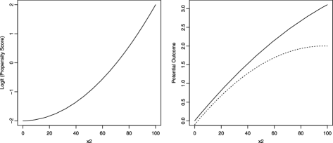
Figure 1: Logit of the propensity score (left) and the potential outcomes [right, solid line $\mathbb{E}\{Y(1)\}$, dashed line $\mathbb{E}\{Y(0)\}$] as a function of $X_{2}$ with $X_{1}=0$ in the simulations.

We generate 500 simulated samples, each consisting of 1000 units. For each unit, we first generate $X_{1}$ and $X_{2}$, and then generate two potential outcomes, and the propensity score, based on which treatment status $Z$ is drawn. For each simulated sample, we apply the semiparametric model selected by CV in comparison to the simple linear specification models $\beta_{0}+\beta_{1}X_{1}+\beta_{2}X_{2}$, for each estimator. The DR estimator has been evaluated also for the two cases where the potential outcomes models or the propensity score model are set to be linear (misspecified). The number of matches in the mixed-matching estimator is set to 6.

Table 1: Average absolute bias (bias), root mean square error (RMSE), and coverage of the 95% confidence interval (coverage) of different estimators in the simulation. The estimators $\hat{\tau}_{\mathrm{dr}}$ (p.s.) and $\hat{\tau}_{\mathrm{dr}}$ (p.o.) represent the (partially misspecified) DR estimator with the propensity score model and the potential outcome model misspecified, respectively. Note that these two estimators, though presented under the “semiparametric” category, are in fact mixed-semiparametric–linear ones

	Semiparametric			Linear
	Bias	RMSE	Coverage	Bias	RMSE	Coverage
$\hat{\tau}_{\mathrm{reg}}$	0.022	0.035	0.889	0.200	0.202	00000
$\hat{\tau}_{\mathrm{wt}}$	0.001	0.058	0.920	0.067	0.077	0.879
$\hat{\tau}_{\mathrm{mix}}$	0.009	0.035	0.939	0.062	0.072	0.697
$\hat{\tau}_{\mathrm{dr}}$	0.003	0.034	0.924	0.144	0.150	0.159
$\hat{\tau}_{\mathrm{dr}}$ (p.s.)	0.016	0.033	0.897	–	–	–
$\hat{\tau}_{\mathrm{dr}}$ (p.o.)	0.008	0.138	0.740	–	–	–

Table 1 reports the absolute bias, root of mean squared error (RMSE), and coverage of the 95% confidence interval of each estimator. Unsurprisingly, the semiparametric specification dominates its linear counterpart for each estimator. Within the semiparametric specification, the weighting and the DR estimator have the smallest biases (0.001 and 0.003, resp.), with DR having a lower RMSE $(0.034)$. Coverage of the 95% confidence intervals are similar between these two estimators (0.920 for $\hat{\tau}_{\mathrm{wt}}$ and 0.924 for $\hat{\tau}_{\mathrm{dr}}$). The mixed-matching estimator gives a larger bias (0.009) but similar RMSE and coverage to those of the DR estimator. The regression estimator gives the biggest bias (0.022) and the lowest coverage (0.889). When only the propensity score model is misspecified, the DR estimator still outperforms both the weighting and the regression estimator. But when both the models are misspecified DR leads to much higher bias and RMSE than the misspecified weighting estimator. The mixed-matching estimator appears to be the least sensitive to misspecifications among the four estimators, especially when there is significant covariate imbalance between treatment groups, as in this simulation. More simulations (omitted here) show this advantage diminishes with increasing covariate balance or decreasing sample size. Finally, the results demonstrate the aforementioned diagnostic potential of the DR estimator: when only the propensity score model is misspecified, the bias from the DR estimator is closer to that obtained from a correctly-specified regression estimator, while when only the potential outcomes model is misspecified, the bias from the DR estimator is closer to that obtained from a correctly-specified weighting estimator.

5 Application to the Italy SHIW data

5.1 Data and preliminary analysis

The SHIW has been run every two years since 1965 with the only exception being that the 1997 survey was delayed to 1998. We denote by $t$ the generic survey year, and by $(t+1)$ the subsequent survey year. We define the target population as the set of households having at least one bank current account but no debit cards at $t$. The treatment $Z$ is posed equal to 1 if, at $t+1$, the household (all members combined) possesses one and only one debit card, equal to 0 if, at $t+1$, the household do not possess debit cards. The households with more than one debit cards are excluded from the sample; therefore, a household for which $Z=1$ is characterized by having acquired their first (and only) debit card during the span $t\rightarrow(t+1)$. Though we do not have exact information of the ownership of the debit cards, it is reasonable to assume that it is the head of the household who possesses the card in most cases. The outcome on which to evaluate the treatment effect is the monthly average spending of the household on all consumer goods and is observed at $t+1$. The pre-treatment variables include the following: the lagged outcome, some background demographic and social variables referred either to the household or to the head householder, the number of banks, and the yearly based average interest rate in the province where the household lives. The subset of pre-treatment variables referred to the household includes the following: the number of earners (four categories), average age of the household (five categories), family size (five categories), the overall household income and wealth, the Italian geographical macro-area where the household lives (three categories), the number of inhabitants of the town where the household lives (four categories), and the monthly average cash inventory held by the household. Those related to the head householder include age (five categories) and education (six categories). All the information is drawn from responses to the SHIW questionnaires with the exception of the number of banks and the average interest rate that are available since 1993 from the Bank of Italy Monetary Statistics. These two variables have been suggested by Attanasio, Guiso and Jappelli (2002), who showed, in a noncausal context and to different purposes, that interest rate and the number of banks in the area where the household lives have a significant contribution to the probability of acquiring a debit card in Italy.

Table 2: Sample sizes and relative frequency of treated and untreated units for each span

	Treated		Untreated
$\bolds{{t\rightarrow(t+1)}}$	Size	Rel. freq.	Size	Rel. freq.	Total
1993–1995	223	0.217	805	0.783	1028
1995–1998	188	0.322	396	0.678	0584
1998–2000	160	0.230	534	0.770	0694

The PATT is estimated by comparing the observed outcomes for the treated units with their predicted counterfactual outcomes. As a consequence, reliable inferences need sufficiently large samples of untreated units where to predict the counterfactual outcomes. SHIW is a repeated cross-section with a panel component, namely, only a part of the sample comprises households that were interviewed in previous surveys. Our analysis will focus on the households observed for two consecutive surveys. Table 2 reports the samples sizes for each span, $t\rightarrow(t+1)$, where $t=1993,95,98$, distinctly by treated and untreated units. The relative frequency of untreated units (the households not possessing debit cards) alongside the total sample size has a considerable drop after 2000. Accordingly, the analysis will be limited to the span until 1998–2000, the latest presenting considerable share of both untreated units and total sample size.

As a preliminary step, we conduct a simple descriptive cross-sectional analysis on the subsample of households observed in a single sweep of the survey. The sample size, shown in the first row of Table 3, is considerably larger than that of the corresponding year in Table 2. The average difference in monthly average spending between households possessing one debit card and households without a debit card is 324.9, 307.8, and 437.3 thousands of Italian Liras (the Italian currency until 2002) in year 1995, 1998, and 2000, respectively. Though not sufficient to establish causal effects of debit cards on spending, this shows that consumers in Italy who possess debit cards spend more compared to those who do not. To explore the characteristics of the households possessing debit cards, we fit a logistic model to this subsample, where the log odds ratio of having one debit card at a certain year is linearly regressed on a set of background demographic and social variables observed at the same year. The variables and their estimated coefficients are shown in Table 3. We observe significant contributions for many of the explanatory variables for each year. In particular, the probability of observing a household that has one debit card increases with income, the town size, education of the head householder, from the South to North of Italy, while it decreases with the average age of the household.

Table 3: MLE of the coefficients ($p$-values in parenthesis) of the logistic model with response variable being the indicator of a household having one debit card

	1995	1998	2000
Sample size	4636	4010	4528
Intercept	$-1.80\ (0.00)$	$-0.02\ (0.96)$	$0.30\ (0.46)$
Income	$1.3\times 10^{-5}$ (0.00)	$3.9\times 10^{-6}$ (0.00)	$7.9\times 10^{-6}$ (0.00)
Wealth	$-4.8\times 10^{-7}$ (0.00)	$-9.0\times 10^{-8}$ (0.19)	$-2.3\times 10^{-7}$ (0.00)
Geographical area (baseline: North):
Center	$-0.46\ (0.00)$	$0.01\ (0.92)$	$-0.15\ (0.18)$
South and Islands	$-0.77\ (0.00)$	$-0.36\ (0.00)$	$-0.60\ (0.00)$
Town size (baseline: $<$20,000):
20,000–40,000	$0.21\ (0.02)$	$-0.04\ (0.64)$	$-0.11\ (0.25)$
40,000–500,000	$0.40\ (0.00)$	$0.13\ (0.12)$	$-0.02\ (0.75)$
$>$500,000	$0.60\ (0.00)$	$0.28\ (0.10)$	$-0.11\ (0.48)$
Family size (baseline: 1):
2	$0.03\ (0.80)$	$0.03\ (0.79)$	$-0.01\ (0.88)$
3	$0.08\ (0.59)$	$0.18\ (0.24)$	$-0.17\ (0.23)$
4	$-0.00\ (0.98)$	$0.03\ (0.84)$	$-0.09\ (0.58)$
$>$4	$-0.14\ (0.46)$	$-0.03\ (0.86)$	$-0.37\ (0.06)$
No. of earners (baseline: 1):
2	$-0.09\ (0.25)$	$-0.04\ (0.62)$	$0.11\ (0.18)$
3	$-0.05\ (0.69)$	$0.12\ (0.41)$	$0.09\ (0.50)$
$>$3	$-0.00\ (0.96)$	$-0.36\ (0.14)$	$-0.05\ (0.81)$
Average age of the household (baseline: $<$31):
31–40	$-0.12\ (0.28)$	$-0.22\ (0.06)$	$-0.25\ (0.04)$
41–50	$-0.23\ (0.11)$	$-0.12\ (0.46)$	$-0.31\ (0.05)$
51–65	$-0.38\ (0.03)$	$-0.31\ (0.11)$	$-0.40\ (0.03)$
$>$65	$-1.09\ (0.00)$	$-0.90\ (0.00)$	$-1.31\ (0.00)$
Education of the head of the household (baseline: none):
Elementary school	$0.31\ (0.12)$	$0.14\ (0.52)$	$0.70\ (0.00)$
Middle school	$0.94\ (0.00)$	$0.68\ (0.00)$	$1.06\ (0.00)$
Prof. 2nd school	$0.98\ (0.00)$	$0.76\ (0.00)$	$1.38\ (0.00)$
High school	$1.32\ (0.00)$	$1.09\ (0.00)$	$1.64\ (0.00)$
University	$1.36\ (0.00)$	$1.19\ (0.00)$	$1.76\ (0.00)$
Age of the head of the household (baseline: $<$31):
31–40	$-0.05\ (0.73)$	$-0.07\ (0.70)$	$0.22\ (0.24)$
41–50	$-0.25\ (0.15)$	$-0.33\ (0.11)$	$-0.10\ (0.60)$
51–65	$-0.40\ (0.04)$	$-0.41\ (0.07)$	$-0.23\ (0.28)$
$>$65	$-0.62\ (0.00)$	$-0.86\ (0.00)$	$-0.48\ (0.04)$
Average interest rate	$0.21\ (0.05)$	$0.07\ (0.68)$	$-0.30\ (0.15)$
Number of banks	$-0.00\ (0.16)$	$0.00\ (0.13)$	$0.00\ (0.31)$

5.2 Model specification

We estimate the propensity score and the potential outcomes according to the semiparametric specification in Section 3.3, where the order term is selected from leave-one-out CV. For both models, the covariates include those listed in Table 3, the cash inventory held by the household, and the lagged outcome from the previous survey. Tables 4 and 5 report the mean squared predicted errors (MSE) for the propensity score, $e(\mathbf{x})$, and the outcome regression, $\mu_{z=0}(\mathbf{x})$, respectively, where $l$ denotes the maximum power term in the power series expansion of the nonparametric part $g(\bolds{\cdot})$ in model (6). The MSE for estimating the propensity score is minimized, for each span, when the continuous pre-treatment variables are posed at the simplest linear specification, $l=1$. We then undersmooth the propensity score specification by expanding $g(\bolds{\cdot})$ to $l=5$. For the outcome model, according to Table 5, we set $l=1$ for the spans 1993–1995 and 1998–2000, and $l=3$ for the span 1995–1998.

=200pt ${\bolds{l}}$ 1993–1995 1995–1998 1998–2000 1 $0.4076^{\ast}$ $0.4748^{\ast}$ $0.4082^{\ast}$ 2 $0.4099$ $0.4771$ $0.4114$ 3 $0.4097$ $0.4808$ $0.4201$ 4 $0.4120$ $0.4862$ $0.4204$ 5 $0.4126$ $0.4886$ $0.4265$

Table 4: MSEs for predicting propensity score $e(\mathbf{x})$, obtained from leave-one-out cross-validation, and ^∗ denotes the minimized MSE

=200pt ${\bolds{l}}$ 1993–1995 1995–1998 1998–2000 1 $544.8^{\ast}$ $597.1$ $1141.8^{\ast}$ 2 $569.8$ $597.9$ $2040.8$ 3 $634.7$ $590.5^{\ast}$ $2.9\cdot e^{5}$ 4 $1230.2$ $592.0$ $7.9\cdot e^{6}$ 5 $2224.7$ $1352.6$ $4.1\cdot e^{7}$

Table 5: MSEs for predicting ${\mu}_{z=0}(\mathbf{x})$, obtained from leave-one-out cross-validation, and ^∗ denotes the minimized MSE

5.3 Assessment of overlap, balance, and unconfoundedness

We assess the overlap assumption by plotting the distribution of the estimated propensity scores in the treatment and control groups and visually inspecting the overlap. Figure 2 presents the histograms of the propensity scores estimated from the semiparametric model (8) for the treated and control groups, which shows a satisfactory overlap in all three spans. Nevertheless, for the purpose of further improving the overlap, we discard the very few units with extreme values of the estimated propensity score: one unit for the span 1993–1995, and four units for the span 1995–1998.

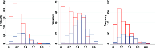
Figure 2: Histograms of the estimated propensity score for the treated (blue) and the untreated (red). The first is for the span 1993 to 1995, the second is for the span 1995 to 1998, and the third is for the span 1998 to 2000.

We further check the balance of covariates based on the estimated propensity score under each estimating method. In particular, we measure covariate balance by the absolute standardized difference (ASD), that is, the absolute difference in the means of the weighted covariate between the treatment and control groups divided by the square root of the sum of within group variances:

$$\operatorname{ASD}={\biggl{|}\frac{\sum_{i=1}^{N}X_{i}Z_{i}w_{i}}{\sum_{i=1}^{N}Z_{i}w_{i}}-\frac{\sum_{i=1}^{N}X_{i}(1-Z_{i})w_{i}}{\sum_{i=1}^{N}(1-Z_{i})w_{i}}\biggr{|}}\Big{/}{\sqrt{s_{1}^{2}/N_{1}+s_{0}^{2}/N_{0}}},$$ (9)

where $N_{z}$ is the number of units and $s_{z}^{2}$ is the standard deviation of the unweighted covariate in group $Z=z$ for $z=0,1$. For the original data (used in the regression estimator $\hat{\tau}_{\mathrm{reg}}$), $w_{i}=1$ for each unit and ASD is the standard two-sample $t$-statistic; for the weighting-based estimators ($\hat{\tau}_{\mathrm{wt}}$ and $\hat{\tau}_{\mathrm{dr}}$), $w_{i}$ are the ATT weights defined before; for the matching-based estimator ($\hat{\tau}_{\mathrm{mix}}$), for each treated unit $w_{i}$ equals 1 and for each control units $w_{i}$ equals the number of that unit being sampled (can be larger than 1 in the case of matching with replacement). The boxplots of the ASD for all covariates from different methods are shown in Figure 3. Weighting leads to substantial improvement in the overall balance of all covariates, with the largest ASD smaller than 1 (1.96 can be viewed as a threshold of significant difference). This can be viewed as evidence that the propensity score is well estimated.

For the mixed matching-regression estimator $\hat{\tau}_{\mathrm{mix}}$, the number of matched units $m$ was set at 6, and the distance metric, $\|\mathbf{x}\|=(\mathbf{x}^{\prime}\mathbf{Sx})^{1/2}$ where $\mathbf{S}$ is the diagonal matrix of the inverses of the covariates variances, is adopted. From the boxplot we can see matching ($m=6$) also improves balance, but significant residual imbalance presents in several variables. Comparing covariate balances and estimated effects obtained from matched samples with different values of $m$ (2 to 6), we noticed a bias-variance trade-off in $\hat{\tau}_{\mathrm{mix}}$: a larger number of matches ($m$) increases residual imbalance in covariates, but at the same time decreases the standard errors of the estimate. Because the regression step in $\hat{\tau}_{\mathrm{mix}}$ can adjust for the residual imbalance, we choose $m=6$ in the SHIW to reduce the standard errors.

Figure 3: Boxplots of the absolute standardized difference of all covariates in the original, weighted, and matched data.

The unconfoundedness assumption is generally untestable, and here we adopt the approach of Crump et al. (2008) to indirectly assess its plausibility via a test based on quantifying the treatment effect on the lagged outcome. The idea is that the lagged outcome, $Y_{\mathrm{lag}}$, can be considered a proxy for $Y(0)$ and, given it is observed before the treatment, it is unaffected by the treatment. Consequently, if the average treatment effect on the lagged outcome is estimated to be zero for all subpopulations defined by the rest of the pre-treatment covariates, $\mathbf{V}=(\mathbf{X}\setminus Y_{\mathrm{lag}})$, then the unconfoundedness assumption is plausible. The hypotheses are formalized as

$$H_{0}\dvtx\mathbb{E}(Y_{\mathrm{lag},z=1}-Y_{\mathrm{lag},z=0}|\mathbf{V}=\mathbf{v})=0\qquad\forall\mathbf{v}\quad\mbox{vs.}$$

$$H_{1}\dvtx\exists\mathbf{v}\mbox{ s.t. }\mathbb{E}(Y_{\mathrm{lag},z=1}-Y_{\mathrm{lag},z=0}|\mathbf{V}=\mathbf{v})\neq 0,$$

and can be tested using the aforementioned power series regression approach to estimation for average treatment effects. In particular, given the order term $k$, the series estimator of the regression function $\mu_{z}(\mathbf{v})$ of the lagged outcome $Y_{\mathrm{lag}}$ under the treatment $z$ ($z=0,1$) is

$$\hat{\mu}_{z}(\mathbf{V})=\mathbf{D}_{k,z}\bigl{(}\mathbf{D}_{k,z}^{\prime}\mathbf{D}_{k,z}\bigr{)}^{-1}\mathbf{D}_{k,z}^{\prime}\tilde{\mathbf{Y}}_{\mathrm{lag},z}=\mathbf{D}_{k,z}\hat{\bolds{\xi}}_{k,z},$$

where $\mathbf{D}_{k,z}=\mathbf{P}_{k}(\tilde{\mathbf{V}}_{z})$, with $\tilde{\mathbf{V}}_{z},\tilde{\mathbf{Y}}_{\mathrm{lag},z}$ being the matrices and the vector of all the observed values of $\mathbf{V},\mathbf{Y}_{\mathrm{lag}}$ in group $z$ and $\mathbf{P}_{k}(\cdot)$ defined as in Section 3.3. Chen (2007) shows that if $k$ increases with the sample size $N$ (even if at a lower rate), the test statistic $Q$ is the quadratic form and converges to a chi-square distribution with $k$ degrees of freedom under the null hypothesis:

$$Q=(\hat{\bolds{\xi}}_{k,1}-\hat{\bolds{\xi}}_{k,0})^{\prime}\hat{\mathbf{S}}_{k}^{-1}(\hat{\bolds{\xi}}_{k,1}-\hat{\bolds{\xi}}_{k,0})\rightarrow\chi^{2}(k),$$

where $\hat{\mathbf{S}}_{k}=\sum_{z}\mathbf{S}_{z}$ with $\mathbf{S}_{z}$ being the estimated limiting variance of $\sqrt{N_{z}}\hat{\bolds{\xi}}_{z,k}$. Therefore, implementation of the test is identical to that of a parametric test for the equality restrictions $\bolds{\xi}_{k,1}=\bolds{\xi}_{k,0}$ in the parametric setting.

Table 6: Results from the tests to assess unconfoundedness

	1993–1995	1995–1998	1998–2000
${l}_{\min\ \mathrm{CV}}$	$3$	$5$	$2$
${k}$	$42$	$52$	$38$
${Q}$	$52.7$	$43.9$	$36.9$
$p$-value	$0.124$	$0.780$	$0.522$

Table 6 shows the values for $Q$ (along with their respective $p$-values) under the null of unconfoundedness, where $l$ is set to $l_{\min\ \mathrm{CV}}$, namely, the maximum power term in the power series expansion of the nonparametric part $g(\bolds{\cdot})$ for which the MSE is minimized. For 1995–1998 and 1998–2000, $l_{\min\ \mathrm{CV}}$ do not coincide for the untreated, $l_{\min\ \mathrm{CV}}=5,1$, respectively, and the treated units, $l_{\min\ \mathrm{CV}}=4,2$. For these two spans, $l_{\min\ \mathrm{CV}}$ has been posed at 5 and 2, respectively, for the regressions $\mu_{z}(\mathbf{v})$ in order to undersmooth the nonparametric specification. The $p$-values for the three periods (0.124, 0.780, 0.522 for period 1993–1995, 1995–1998, 1998–2000, resp.) suggest that there is no difference in the lagged outcome between groups and, consequently, the unconfoundedness assumption is deemed plausible.

Table 7: Estimated PATT in thousands of Italian Lira (standard errors in parenthesis)

		$\bolds{\hat{\tau}_{\mathrm{reg}}}$		$\bolds{\hat{\tau}_{\mathrm{wt}}}$		$\bolds{\hat{\tau}_{\mathrm{mix}}}$		$\bolds{\hat{\tau}_{\mathrm{dr}}}$
Span	AOT	PATT	$\frac{\mbox{{PATT}}}{\mbox{{AOT}}}$	PATT	$\frac{\mbox{{PATT}}}{\mbox{{AOT}}}$	PATT	$\frac{\mbox{{PATT}}}{\mbox{{AOT}}}$	PATT	$\frac{\mbox{{PATT}}}{\mbox{{AOT}}}$
1993–1995	2092.9	90.2	0.043	102.3	0.049	100.6	0.048	97.2	0.046
		(41.8)		(47.1)		(50.4)		(42.7)
1995–1998	2027.6	199.1	0.098	160.7	0.079	208.7	0.103	202.2	0.100
		(87.6)		(73.4)		(69.8)		(93.2)
1998–2000	2116.4	148.1	0.069	137.7	0.065	122.8	0.058	142.1	0.067
		(68.5)		(73.1)		(60.7)		(70.5)

5.4 Results

We obtain results from the regression estimator $\hat{\tau}_{\mathrm{reg}}$, the propensity score weighting estimator $\hat{\tau}_{\mathrm{wt}}$, and the DR estimator $\hat{\tau}_{\mathrm{dr}}$ by using common routines for linear and logistic regressions in STATA and GAUSS. Point estimates and standard errors from the mixed matching-regression estimator $\hat{\tau}_{\mathrm{mix}}$ have been obtained by the STATA program by Abadie et al. (2003).

Table 7 reports the effects of debit cards on household monthly consumption estimated from the four estimators. The ratios between each estimated PATT and the Average Outcome for the Treated (AOT) are also reported. Positive and statistically significant estimates of the PATT are consistently obtained across all estimators and all spans. For the span of 1993–1995, the increase in the monthly consumption for the household with one debit card ranges from 4.3% to 4.9% (90.2 to 100.6 thousands Italian Liras) across the four estimators; for the span of 1998–2000, the increase ranges from 5.8% to 6.9% (122.8 to 148.1 thousands Liras). The period 1995–1998 emerges with particular high estimated PATT, ranging from 7.9% (160.7 thousands Liras) to 10.3% (208.7 thousands Liras) of the household monthly consumption. This can be explained by the fact that the period was observed one year longer (the planned survey for 1997 was delayed one year and shifted to 1998); therefore, the use of debit cards could have benefited from the longer span to more strongly affect consumers’ behavior. Note that in the span of 1995–1998, the weighting estimate is significantly different from both the regression and the DR estimates, suggesting a potential misspecification of the propensity score.

Overall, these results support current psychological theories about the effects of debit cards on spending. As debit cards do not allow the consumer to incorporate an additional long-term source of funds, our analysis largely eliminates the potential confounded effect of an intertemporal reallocation of wealth [Soman and Cheema (2002)]. Therefore, the significant estimated effects on spending can be ascribed only to psychological reasons, in particular, those pertaining to the aforementioned theories regarding the rehearsal of the price paid [Soman (2001)] and regarding the accessibility of financial resources [Morewedge, Hotzman and Epley (2007)]. Both theories state that payments by debit cards enlarge the perceived amount of financial resources available for consumption compared to pay cash. This is due, in one case, to an impact on the memory of past expenses and, in the other case, to the cognitive accessibility to a larger financial resource like the savings account. Our findings can be explained by the microeconomic theory of consumer choice in that the perception of larger disposable financial resources implies less budget constraints. This enlarges the set of affordable bundles and increases the ordinary demand because the most preferred affordable bundle, that is, the rational consumer’s choice, will be composed by a larger quantity of goods for rational utility functions. This is essentially an income effect; however, if the occasions to pay by debit cards differ by categories of goods, also a substitution effect will be in act. The latter could be studied by evaluating the effect on spending for different categories of goods, for example, for food versus nonfood consumption.

6 Conclusion

Motivated by recent findings in the field of consumer science, we conduct a population-based study based on the Italy SHIW data to evaluate the causal effect of debit cards on household consumption. Within the RCM, we adopt several power series-based semiparametric approaches to estimate the PATT. The key assumptions, overlap and unconfoundedness, are systematically assessed and validated. Our analysis suggests that possessing debit cards significantly increases monthly household spending in Italy, consistent with and complementary to the findings from several small randomized experiments in psychology and consumer science.

One limitation of the study is that only short-time effects of the considered payment instrument have been here evaluated. In fact, the SHIW data do not provide information about the moment a treated household has acquired its debit cards. We only know it has happened during the two, or three, years of the considered span, so that we have likely estimated one to one-and-a-half years long effects. A desirable extension of this work may be to apply the same causal methods to suitable data sets that allow for enlarging the extent of the temporal effects of debit cards. Another limitation is that, due to data availability, this study focuses on household rather than individual spending. This problem is partially mitigated by restricting the analysis to households with one and only one debit card. Nevertheless, an analysis on singleton households or households formed only by a couple or population-based data with individual information would provide more information.

We have focused on the PATT estimand; other estimands may be of interest depending on the study goal. For example, if the goal were to plan a marketing policy aimed to increase spending by stimulating the use of noncash payment instruments, then the relevant causal effect should be on untreated units. Consequently, the estimators considered here need to be modified accordingly.

Appendix: Proof of the “double robustness” property of the estimator $\hat{\tau}_{\mathrm{dr}}$

It is trivial to prove the first term of (5), $\sum_{i=1}^{N}Y_{i}Z_{i}/\sum_{i=1}^{N}Z_{i}$, converges to $\mathbb{E}\{Y(1)|Z=1\}$.

For the second term, first suppose the outcome model $\mu_{0}(\mathbf{X})$ is correctly specified but the propensity score $e(\mathbf{X})$ is misspecified, so that $\hat{\mu}_{0}(\mathbf{X})\rightarrow\mathbb{E}(Y(0)|\mathbf{X})$, $\hat{e}(\mathbf{X})\nrightarrow\Pr(Z=1|\mathbf{X})$. Then we have

$$\frac{1}{\sum_{i=1}^{N}Z_{i}}\sum_{i=1}^{N}\frac{Y_{i}(1-Z_{i})\hat{e}(\mathbf{X}_{i})+\hat{\mu}_{0}(\mathbf{X}_{i})(Z_{i}-\hat{e}(\mathbf{X}_{i}))}{1-\hat{e}(\mathbf{X}_{i})}$$

$$\qquad=\frac{1}{\sum_{i=1}^{N}Z_{i}}\biggl{\{}\sum_{i:Z_{i}=1}\hat{\mu}_{0}(\mathbf{X}_{i})+\sum_{i:Z_{i}=0}\frac{Y_{i}\hat{e}(\mathbf{X}_{i})-\hat{\mu}_{0}(\mathbf{X}_{i})\hat{e}(\mathbf{X}_{i})}{1-\hat{e}(\mathbf{X}_{i})}\biggr{\}}$$

(10)

$$\qquad=\frac{1}{\sum_{i=1}^{N}Z_{i}}\sum_{i:Z_{i}=1}\hat{\mu}_{0}(\mathbf{X}_{i})$$

$$\qquad\quad{}+\frac{\sum_{i=1}^{N}(1-Z_{i})}{\sum_{i=1}^{N}Z_{i}}\frac{1}{\sum_{i=1}^{N}(1-Z_{i})}\sum_{i:Z_{i}=0}\biggl{\{}\frac{Y_{i}\hat{e}(\mathbf{X}_{i})}{1-\hat{e}(\mathbf{X}_{i})}-\frac{\hat{\mu}_{0}(\mathbf{X}_{i})\hat{e}(\mathbf{X}_{i})}{1-\hat{e}(\mathbf{X}_{i})}\biggr{\}}.$$

It is straightforward to prove, given the law of large numbers and the consistency of $\hat{\mu}_{0}(\mathbf{X})$, that $\sum_{i:Z_{i}=1}\hat{\mu}_{0}(\mathbf{X}_{i})/\sum_{i=1}^{N}Z_{i}$ converges to $\mathbb{E}_{\mathbf{X}}\{\mathbb{E}(Y(0)|\mathbf{X})|\break Z=1\}$, and $\sum_{i:Z_{i}=0}\frac{Y_{i}\hat{e}(\mathbf{X}_{i})}{1-\hat{e}(\mathbf{X}_{i})}/{\sum_{i=1}^{N}(1-Z_{i})}$ and $\sum_{i:Z_{i}=0}\frac{\hat{\mu}_{0}(\mathbf{X}_{i})\hat{e}(\mathbf{X}_{i})}{1-\hat{e}(\mathbf{X}_{i})}/\break{\sum_{i=1}^{N}(1-Z_{i})}$ converge to the same quantity $\mathbb{E}_{\mathbf{X}}\{\mathbb{E}(Y(0)|\mathbf{X})\frac{\hat{e}(\mathbf{X})}{1-\hat{e}(\mathbf{X})}|Z=0\}$. Consequently, equation (Appendix: Proof of the “double robustness” property of the estimator $\hat{\tau}_{\mathrm{dr}}$) converges to (the subscript $i$ is dropped to simplify the notation)

$$\mathbb{E}_{\mathbf{X}}\bigl{\{}\mathbb{E}\bigl{(}Y(0)|\mathbf{X}\bigr{)}|Z=1\bigr{\}} = \int_{\mathbf{x}}f(\mathbf{x}|Z=1)\mathbb{E}\bigl{\{}Y(0)|\mathbf{X}=\mathbf{x}\bigr{\}}$$

$$= \int_{\mathbf{x}}f(\mathbf{x}|Z=1)\mathbb{E}\bigl{\{}Y(0)|\mathbf{X}=\mathbf{x},Z=1\bigr{\}}$$

$$= \int_{\mathbf{x}}f(\mathbf{x}|Z=1)\int_{y(0)}y(0)f\bigl{(}y(0)|\mathbf{X}=\mathbf{x},Z=1\bigr{)}$$

$$= \int_{y(0)}y(0)f\bigl{(}y(0)|Z=1\bigr{)}$$

$$= \mathbb{E}\bigl{\{}Y(0)|Z=1\bigr{\}}.$$

Above, the second equation is due to the unconfoundedness assumption.

Alternatively, suppose $e(\mathbf{X})$ is correctly specified while $\mu_{0}(\mathbf{X})$ is misspecified, so that $\hat{e}(\mathbf{X})\rightarrow\Pr(Z=1|\mathbf{X})$, $\hat{\mu}_{0}(\mathbf{X})\nrightarrow\mathbb{E}(Y(0)|\mathbf{X})$. Again, it is easy to prove, given the law of large numbers and the consistency of $\hat{e}(\mathbf{X}_{i})$, that the quantities $\sum_{i:Z_{i}=1}\hat{\mu}_{0}(\mathbf{X}_{i})/{\sum_{i=1}^{N}Z_{i}}$ and $\frac{\sum_{i=1}^{N}(1-Z_{i})}{\sum_{i=1}^{N}Z_{i}}\frac{1}{\sum_{i=1}^{N}(1-Z_{i})}\times\break\sum_{i:Z_{i}=0}\{\frac{\hat{\mu}_{0}(\mathbf{X}_{i})\hat{e}(\mathbf{X}_{i})}{1-\hat{e}(\mathbf{X}_{i})}\}$ converge to the same quantity $\mathbb{E}_{\mathbf{X}}\{\hat{\mu}_{0}(\mathbf{X})|Z=0\}$, and $\frac{\sum_{i=1}^{N}(1-Z_{i})}{\sum_{i=1}^{N}Z_{i}}\frac{1}{\sum_{i=1}^{N}(1-Z_{i})}\sum_{i:Z_{i}=0}\{\frac{Y_{i}\hat{e}(\mathbf{X}_{i})}{1-\hat{e}(\mathbf{X}_{i})}\}$ converges to $\frac{\Pr(Z=0)}{\Pr(Z=1)}\mathbb{E}_{\mathbf{X}}\{\frac{\Pr(Z=1|\mathbf{X})}{\Pr(Z=0|\mathbf{X})}\times\break\mathbb{E}(Y(0)|\mathbf{X})|Z=0\}$. Consequently, equation (Appendix: Proof of the “double robustness” property of the estimator $\hat{\tau}_{\mathrm{dr}}$) converges to

$$\frac{\Pr(Z=0)}{\Pr(Z=1)}\mathbb{E}_{\mathbf{X}}\biggl{\{}\frac{\Pr(Z=1|\mathbf{X}=\mathbf{x})}{\Pr(Z=0|\mathbf{X}=\mathbf{x})}\mathbb{E}\bigl{(}Y(0)|\mathbf{X}\bigr{)}|Z=0\biggr{\}}$$

$$\qquad=\frac{\Pr(Z=0)}{\Pr(Z=1)}\int_{\mathbf{x}}f(\mathbf{x}|Z=0)\frac{\Pr(Z=1|\mathbf{X}=\mathbf{x})}{\Pr(Z=0|\mathbf{X}=\mathbf{x})}\int_{y(0)}y(0)f\bigl{(}y(0)|\mathbf{X}=\mathbf{x}\bigr{)}$$

$$\qquad=\int_{\mathbf{x}}f(\mathbf{x}|Z=0)\frac{f(\mathbf{x}|Z=1)}{f(\mathbf{x}|Z=0)}\int_{y(0)}y(0)f\bigl{(}y(0)|\mathbf{X}=\mathbf{x},Z=1\bigr{)}$$

$$\qquad=\int_{y(0)}y(0)\int_{\mathbf{x}}f(\mathbf{x}|Z=1)f\bigl{(}y(0)|\mathbf{X}=\mathbf{x},Z=1\bigr{)}$$

$$\qquad=\int_{y(0)}y(0)f\bigl{(}y(0)|Z=1\bigr{)}=\mathbb{E}\bigl{\{}Y(0)|Z=1\bigr{\}}.$$

The same arguments apply to the case of both $\mu_{0}(\mathbf{X})$ and $e(\mathbf{X})$ correctly specified. Then, $\hat{\tau}_{\mathrm{dr}}$ converges to $\mathbb{E}\{Y(1)|Z=1\}-\mathbb{E}\{Y(0)|Z=1\}=\tau^{\mathrm{PATT}}$ when the outcome model $\mu_{0}(\mathbf{X})$ and/or the propensity score model $e(\mathbf{X})$ are correctly specified. ∎

References

- Abadie and Imbens (2006) {barticle}[mr] \bauthor\bsnmAbadie, \bfnmAlberto\binitsA. and \bauthor\bsnmImbens, \bfnmGuido W.\binitsG. W. (\byear2006). \btitleLarge sample properties of matching estimators for average treatment effects. \bjournalEconometrica \bvolume74 \bpages235–267. \biddoi=10.1111/j.1468-0262.2006.00655.x, issn=0012-9682, mr=2194325 \bptokimsref\endbibitem
- Abadie and Imbens (2011) {barticle}[mr] \bauthor\bsnmAbadie, \bfnmAlberto\binitsA. and \bauthor\bsnmImbens, \bfnmGuido W.\binitsG. W. (\byear2011). \btitleBias-corrected matching estimators for average treatment effects. \bjournalJ. Bus. Econom. Statist. \bvolume29 \bpages1–11. \biddoi=10.1198/jbes.2009.07333, issn=0735-0015, mr=2789386 \bptokimsref\endbibitem
- Abadie et al. (2003) {barticle}[auto:parserefs-M02] \bauthor\bsnmAbadie, \bfnmA.\binitsA., \bauthor\bsnmDrukker, \bfnmD.\binitsD., \bauthor\bsnmHerr, \bfnmJ. L.\binitsJ. L. and \bauthor\bsnmImbens, \bfnmG. W.\binitsG. W. (\byear2003). \btitleImplementing matching estimators for average treatment effects in Stata. \bjournalThe Stata Journal \bvolume4 \bpages290–311. \bptokimsref\endbibitem
- Attanasio, Guiso and Jappelli (2002) {barticle}[auto:parserefs-M02] \bauthor\bsnmAttanasio, \bfnmO.\binitsO., \bauthor\bsnmGuiso, \bfnmL.\binitsL. and \bauthor\bsnmJappelli, \bfnmT.\binitsT. (\byear2002). \btitleThe demand for money, financial innovation and the welfare cost of inflation: An analysis with household data. \bjournalJournal of Political Economy \bvolume110 \bpages318–351. \bptokimsref\endbibitem
- Burman (1974) {barticle}[auto:parserefs-M02] \bauthor\bsnmBurman, \bfnmD.\binitsD. (\byear1974). \btitleDo people overspend with credit cards? \bjournalThe Journal of Consumer Credit Management \bvolume5 \bpages98–103. \bptokimsref\endbibitem
- Chen (2007) {bincollection}[auto:parserefs-M02] \bauthor\bsnmChen, \bfnmX.\binitsX. (\byear2007). \btitleLarge sample sieve estimation of semi-nonparametric models. In \bbooktitleHandbook of Econometrics 6 (\beditor\bfnmJ.\binitsJ. \bsnmHeckman and \beditor\bfnmE.\binitsE. \bsnmLeamer, eds.) \bpages5549–5632. \bpublisherElsevier Science, \blocationNew York. \bptokimsref\endbibitem
- Cole (1998) {binproceedings}[auto:parserefs-M02] \bauthor\bsnmCole, \bfnmC.\binitsC. (\byear1998). \btitleIdentifying intervetions to reduce credit card misuse through consumer behavior research. In \bbooktitleProc. of the Marketing and Public Policy Conference \bpages11–13. \bpublisherGeorgetown Univ. Press, \blocationWashington, DC. \bptokimsref\endbibitem
- Committee on Payment and Settlement System (2001) {bmisc}[auto:parserefs-M02] \borganizationCommittee on Payment and Settlement System (\byear2001). \bhowpublishedA Glossary of Terms Used in Payments and Settlement Systems. Bank for International Settlements, Basel, Switzerland. \bptokimsref\endbibitem
- Crump et al. (2008) {barticle}[auto:parserefs-M02] \bauthor\bsnmCrump, \bfnmR. K.\binitsR. K., \bauthor\bsnmHotz, \bfnmV. J.\binitsV. J., \bauthor\bsnmImbens, \bfnmG. W.\binitsG. W. and \bauthor\bsnmMitnik, \bfnmO. A.\binitsO. A. (\byear2008). \btitleNonparametric tests for treatment effect heterogeneity. \bjournalThe Review of Economics and Statistics \bvolume90 \bpages389–405. \bptokimsref\endbibitem
- Das, Newey and Vella (2003) {barticle}[mr] \bauthor\bsnmDas, \bfnmMitali\binitsM., \bauthor\bsnmNewey, \bfnmWhitney K.\binitsW. K. and \bauthor\bsnmVella, \bfnmFrancis\binitsF. (\byear2003). \btitleNonparametric estimation of sample selection models. \bjournalRev. Econom. Stud. \bvolume70 \bpages33–58. \biddoi=10.1111/1467-937X.00236, issn=0034-6527, mr=1952565 \bptokimsref\endbibitem
- Feinberg (1986) {barticle}[auto:parserefs-M02] \bauthor\bsnmFeinberg, \bfnmR. A.\binitsR. A. (\byear1986). \btitleCredits cards as spending facilitating stimuli: A conditioning interpretation. \bjournalJournal of Consumer Research \bvolume13 \bpages348–356. \bptokimsref\endbibitem
- Hahn (1998) {barticle}[mr] \bauthor\bsnmHahn, \bfnmJinyong\binitsJ. (\byear1998). \btitleOn the role of the propensity score in efficient semiparametric estimation of average treatment effects. \bjournalEconometrica \bvolume66 \bpages315–331. \biddoi=10.2307/2998560, issn=0012-9682, mr=1612242 \bptokimsref\endbibitem
- Hausman and Newey (1995) {barticle}[auto:parserefs-M02] \bauthor\bsnmHausman, \bfnmJ. A.\binitsJ. A. and \bauthor\bsnmNewey, \bfnmW. K.\binitsW. K. (\byear1995). \btitleNonparametric estimation of exact consumers surplus and deadweight loss. \bjournalEconometrica \bvolume63 \bpages1445–1476. \bptokimsref\endbibitem
- Heat and Soll (1996) {barticle}[auto:parserefs-M02] \bauthor\bsnmHeat, \bfnmC.\binitsC. and \bauthor\bsnmSoll, \bfnmJ. B.\binitsJ. B. (\byear1996). \btitleMental budgeting and consumer decisions. \bjournalJournal of Consumer Research \bvolume23 \bpages40–52. \bptokimsref\endbibitem
- Heckman, Ichimura and Todd (19978) {barticle}[mr] \bauthor\bsnmHeckman, \bfnmJames J.\binitsJ. J., \bauthor\bsnmIchimura, \bfnmHidehiko\binitsH. and \bauthor\bsnmTodd, \bfnmPetra\binitsP. (\byear1997). \btitleMatching as an econometric evaluation estimator: Evidence from a job training program. \bjournalRev. Econom. Stud. \bvolume64 \bpages605–654. \bptokimsref\endbibitem
- Helson (1964) {bbook}[auto:parserefs-M02] \bauthor\bsnmHelson, \bfnmH.\binitsH. (\byear1964). \btitleAdaptation-Level Theory. \bpublisherHarper & Row, \blocationNew York. \bptokimsref\endbibitem
- Hirano and Imbens (2001) {barticle}[auto:parserefs-M02] \bauthor\bsnmHirano, \bfnmK.\binitsK. and \bauthor\bsnmImbens, \bfnmG. W.\binitsG. W. (\byear2001). \btitleEstimation of causal effects using propensity score weighting: An application to data on right heart catheterization. \bjournalHealth Services and Outcomes Research Methodology \bvolume2 \bpages259–278. \bptokimsref\endbibitem
- Hirano, Imbens and Ridder (2003) {barticle}[mr] \bauthor\bsnmHirano, \bfnmKeisuke\binitsK., \bauthor\bsnmImbens, \bfnmGuido W.\binitsG. W. and \bauthor\bsnmRidder, \bfnmGeert\binitsG. (\byear2003). \btitleEfficient estimation of average treatment effects using the estimated propensity score. \bjournalEconometrica \bvolume71 \bpages1161–1189. \biddoi=10.1111/1468-0262.00442, issn=0012-9682, mr=1995826 \bptokimsref\endbibitem
- Hirschman (1979) {barticle}[auto:parserefs-M02] \bauthor\bsnmHirschman, \bfnmE.\binitsE. (\byear1979). \btitleDifferences in consumer purchase behavior by credit card payment system. \bjournalJournal of Consumer Research \bvolume6 \bpages58–66. \bptokimsref\endbibitem
- Holland (1986) {barticle}[mr] \bauthor\bsnmHolland, \bfnmPaul W.\binitsP. W. (\byear1986). \btitleStatistics and causal inference. \bjournalJ. Amer. Statist. Assoc. \bvolume81 \bpages945–970. \bidissn=0162-1459, mr=0867618 \bptnotecheck related \bptokimsref\endbibitem
- Horvitz and Thompson (1952) {barticle}[mr] \bauthor\bsnmHorvitz, \bfnmD. G.\binitsD. G. and \bauthor\bsnmThompson, \bfnmD. J.\binitsD. J. (\byear1952). \btitleA generalization of sampling without replacement from a finite universe. \bjournalJ. Amer. Statist. Assoc. \bvolume47 \bpages663–685. \bidissn=0162-1459, mr=0053460 \bptokimsref\endbibitem
- Hsee et al. (1999) {barticle}[auto:parserefs-M02] \bauthor\bsnmHsee, \bfnmC. K.\binitsC. K., \bauthor\bsnmLoewenstein, \bfnmG. F.\binitsG. F., \bauthor\bsnmBlount, \bfnmS.\binitsS. and \bauthor\bsnmBazerman, \bfnmM. H.\binitsM. H. (\byear1999). \btitlePreference reversals between joint and separate evaluation of options: A review and theoretical analysis. \bjournalPsychological Bullettin \bvolume125 \bpages576–590. \bptokimsref\endbibitem
- Ichino, Mealli and Nannicini (2008) {barticle}[mr] \bauthor\bsnmIchino, \bfnmAndrea\binitsA., \bauthor\bsnmMealli, \bfnmFabrizia\binitsF. and \bauthor\bsnmNannicini, \bfnmTommaso\binitsT. (\byear2008). \btitleFrom temporary help jobs to permanent employment: What can we learn from matching estimators and their sensitivity? \bjournalJ. Appl. Econometrics \bvolume23 \bpages305–327. \biddoi=10.1002/jae.998, issn=0883-7252, mr=2420362 \bptokimsref\endbibitem
- Imbens (2004) {barticle}[auto:parserefs-M02] \bauthor\bsnmImbens, \bfnmG. W.\binitsG. W. (\byear2004). \btitleNonparametric estimation of average treatment effects under exogeneity: A review. \bjournalReview of Economics and Statistics \bvolume86 \bpages4–29. \bptokimsref\endbibitem
- Imbens, Newey and Ridder (2005) {bmisc}[auto:parserefs-M02] \bauthor\bsnmImbens, \bfnmG. W.\binitsG. W., \bauthor\bsnmNewey, \bfnmW.\binitsW. and \bauthor\bsnmRidder, \bfnmG.\binitsG. (\byear2005). \bhowpublishedMean-square-error calculations for average treatment effects. Working Paper 05-34, IEPR. \bptokimsref\endbibitem
- Kahneman and Miller (1986) {barticle}[auto:parserefs-M02] \bauthor\bsnmKahneman, \bfnmD.\binitsD. and \bauthor\bsnmMiller, \bfnmD. T.\binitsD. T. (\byear1986). \btitleNorm theory: Comparing reality to its alternatives. \bjournalPsychological Review \bvolume93 \bpages136–153. \bptokimsref\endbibitem
- Li, Morgan and Zaslavsky (2014) {bmisc}[auto:parserefs-M02] \bauthor\bsnmLi, \bfnmF.\binitsF., \bauthor\bsnmMorgan, \bfnmL. K.\binitsL. K. and \bauthor\bsnmZaslavsky, \bfnmA. M.\binitsA. M. (\byear2014). \bhowpublishedBalancing covariates via propensity score weighting. Available at \arxivurlarXiv:1404.1785. \bptokimsref\endbibitem
- Mann (2006) {bbook}[auto:parserefs-M02] \bauthor\bsnmMann, \bfnmR. J.\binitsR. J. (\byear2006). \btitleCharging Ahead: The Growth and Regulation of Payment Card Markets Around the World. \bpublisherCambridge Univ. Press, \blocationCambridge. \bptokimsref\endbibitem
- Morewedge, Hotzman and Epley (2007) {barticle}[auto:parserefs-M02] \bauthor\bsnmMorewedge, \bfnmC. K.\binitsC. K., \bauthor\bsnmHotzman, \bfnmL.\binitsL. and \bauthor\bsnmEpley, \bfnmN.\binitsN. (\byear2007). \btitleUnfixed resources: Perceived costs, consumption, and the accessible account effect. \bjournalJournal of Consumer Research \bvolume34 \bpages459–467. \bptokimsref\endbibitem
- Parducci (1995) {bbook}[auto:parserefs-M02] \bauthor\bsnmParducci, \bfnmA.\binitsA. (\byear1995). \btitleHappiness, Pleasure and Judgment: The Contextual Theory and Its Application. \bpublisherLawrence Erlbaum Associates, \blocationMahwah, NJ. \bptokimsref\endbibitem
- Prelec and Loewenstein (1998) {barticle}[auto:parserefs-M02] \bauthor\bsnmPrelec, \bfnmD.\binitsD. and \bauthor\bsnmLoewenstein, \bfnmG. F.\binitsG. F. (\byear1998). \btitleThe red and the black: Mental accounting of savings and debt. \bjournalMarketing Science \bvolume17 \bpages4–28. \bptokimsref\endbibitem
- Prelec and Simester (2001) {barticle}[auto:parserefs-M02] \bauthor\bsnmPrelec, \bfnmD.\binitsD. and \bauthor\bsnmSimester, \bfnmD.\binitsD. (\byear2001). \btitleAlways leave home without it: A further investigation of the credit-card effect on willingness to pay. \bjournalMarketing Letters \bvolume12 \bpages5–12. \bptokimsref\endbibitem
- Robins, Rotnitzky and Zhao (1995) {barticle}[mr] \bauthor\bsnmRobins, \bfnmJames M.\binitsJ. M., \bauthor\bsnmRotnitzky, \bfnmAndrea\binitsA. and \bauthor\bsnmZhao, \bfnmLue Ping\binitsL. P. (\byear1995). \btitleAnalysis of semiparametric regression models for repeated outcomes in the presence of missing data. \bjournalJ. Amer. Statist. Assoc. \bvolume90 \bpages106–121. \bidissn=0162-1459, mr=1325118 \bptokimsref\endbibitem
- Rosenbaum and Rubin (1983) {barticle}[mr] \bauthor\bsnmRosenbaum, \bfnmPaul R.\binitsP. R. and \bauthor\bsnmRubin, \bfnmDonald B.\binitsD. B. (\byear1983). \btitleThe central role of the propensity score in observational studies for causal effects. \bjournalBiometrika \bvolume70 \bpages41–55. \biddoi=10.1093/biomet/70.1.41, issn=0006-3444, mr=0742974 \bptokimsref\endbibitem
- Rubin (1974) {barticle}[auto:parserefs-M02] \bauthor\bsnmRubin, \bfnmD. B.\binitsD. B. (\byear1974). \btitleEstimating causal effects of treatments in randomized and nonrandomized studies. \bjournalJournal of Educational Psycology \bvolume66 \bpages688–701. \bptokimsref\endbibitem
- Rubin (1977) {barticle}[auto:parserefs-M02] \bauthor\bsnmRubin, \bfnmD. B.\binitsD. B. (\byear1977). \btitleAssignment to treatment group on the basis of a covariate. \bjournalJournal of Educational Statistics \bvolume2 \bpages1–26. \bptokimsref\endbibitem
- Rubin (1978) {barticle}[mr] \bauthor\bsnmRubin, \bfnmDonald B.\binitsD. B. (\byear1978). \btitleBayesian inference for causal effects: The role of randomization. \bjournalAnn. Statist. \bvolume6 \bpages34–58. \bidissn=0090-5364, mr=0472152 \bptokimsref\endbibitem
- Rubin (1980) {barticle}[mr] \bauthor\bsnmRubin, \bfnmD. B.\binitsD. B. (\byear1980). \btitleDiscussion of “Randomization analysis of experimental data: The Fisher randomization test” by D. Basu. \bjournalJ. Amer. Statist. Assoc. \bvolume75 \bpages591–593. \bptnotecheck related \bptokimsref\endbibitem
- Soman (2001) {barticle}[auto:parserefs-M02] \bauthor\bsnmSoman, \bfnmD.\binitsD. (\byear2001). \btitleEffects of payment mechanism on spending behavior: The role of rehearsal and immediacy of payments. \bjournalJournal of Consumer Research \bvolume27 \bpages460–474. \bptokimsref\endbibitem
- Soman and Cheema (2002) {barticle}[auto:parserefs-M02] \bauthor\bsnmSoman, \bfnmD.\binitsD. and \bauthor\bsnmCheema, \bfnmA.\binitsA. (\byear2002). \btitleThe effects of credit on spending decisions: The role of credit limt and credibility. \bjournalMarketing Science \bvolume21 \bpages32–53. \bptokimsref\endbibitem
- Thaler (1985) {barticle}[auto:parserefs-M02] \bauthor\bsnmThaler, \bfnmR. H.\binitsR. H. (\byear1985). \btitleMental accounting and consumer choice. \bjournalMarketing Science \bvolume4 \bpages199–214. \bptokimsref\endbibitem
- Thaler (1999) {barticle}[auto:parserefs-M02] \bauthor\bsnmThaler, \bfnmR. H.\binitsR. H. (\byear1999). \btitleMental accounting matter. \bjournalJournal of Behavioral Decision Making \bvolume12 \bpages183–206. \bptokimsref\endbibitem
- Tokunaga (1993) {barticle}[auto:parserefs-M02] \bauthor\bsnmTokunaga, \bfnmH.\binitsH. (\byear1993). \btitleThe use and abuse of consumer credit: Applications of psychological theory and research. \bjournalJournal of Economic Psychology \bvolume14 \bpages285–316. \bptokimsref\endbibitem