Screening of quark-monopole in $\mathcal{N}=4$ plasma

Abstract

We study a quark-monopole bound system moving in $\mathcal{N}=4$ SYM plasma with a constant velocity by the AdS/CFT correspondence. The screening length of this system is calculated, and is smaller than that of the quark-antiquark bound state.

September 2014

1 Introduction

The gauge/gravity duality [1] is a useful tool to study the physics of quark gluon plasma (QGP). There are many successful research results along this line. In [2]-[9] etc., the shear viscosity is calculated by this technique. The jet quenching parameter, originally defined in the phenomenological study of energy loss of a heavy quark passing through QGP, can be described and computed nonperturbatively [10] in the AdS/CFT context. Another interesting issue related to energy loss is the drag force experienced by a heavy quark moving in the $\mathcal{N}=4$ supersymmetric Yang-Mills (SYM) plasma, which was first calculated in [11] for a test string dangling from the boundary of AdS-Schwarzchild background to the black hole horizon.

Apart from the remarkable jet quenching phenomenon occurred in hadronization of a single quark, experimentally one also observed that the production of $J/\psi$ mesons in QGP, when compared to that in proton-proton or proton-nucleus collisions, is suppressed [12]. Such suppression could be predicted from phenomenological considerations, since the attractive force between a quark $q$ and an anti-quark $\bar{q}$ should be screened in a deconfined QGP, and the screened interaction would not bind that $q\bar{q}$ bound state. In lattice QCD, however, it is difficult to carry out computations for the screening length $L_{s}$ of a $q\bar{q}$ pair produced in QGP with a high velocity. The AdS/CFT proposal [13] (see also [14] ) now provides a calculable way of determining $L_{s}$ (and the binding energy of the moving $q\bar{q}$ system as well), in $\mathcal{N}=4$ SYM plasma. This study was generalized to other spacetime dimensions in the ultra-relativistic limit [15]. For more related references one can see the review [16].

To get a better understanding of the screening effect in SYM plasma, it would be worthwhile to consider the screening lengths of some bound systems other than the $q\bar{q}$ system. In the $q\bar{q}$ case one finds $L_{s}\propto f(v)(1-v^{2})^{1/4}$, where $f(v)$ is a function depending mildly on the velocity of the plasma wind [13]. A qualitative explanation of why $L_{s}$ contains the factor $(1-v^{2})^{1/4}$ is that the screening length should scale as (energy density)^-1/4, and the energy density will go like $(1-v^{2})^{-1}$ when the wind velocity gets boosted [13]. As argued in [15], this scaling behavior is closely related to the conformal symmetry of $\mathcal{N}=4$ SYM. Thus, one expects that $(1-v^{2})^{1/4}$ is a kind of ”kinetic” factor, which should be seen in any bound systems in the hot $\mathcal{N}=4$ SYM plasma, and the remaining $v$-dependent factor $f(v)$ should depends on the dynamical details of the system.

In this paper, we present a concrete test of the above prediction, by studying screening of a quark-monopole bound system moving with a constant velocity $v$ in a thermal $\mathcal{N}=4$ SYM plasma. At zero temperature a quark of mass $M_{q}$ can bind with a monopole of mass $M_{m}=M_{q}/g$ to form a dyon, which has the mass $M=M_{q}\sqrt{1+1/g^{2}}$ and is smaller than the total mass $M_{q}+M_{m}=M_{q}(1+1/g)$ of a free quark and a free monopole (here $g=g_{\rm YM}^{2}/{4\pi}$ is the string coupling constant). Such a bound system is not too heavy compared to the quark mass provided we live in a strong coupling regime ($g\sim 1$). The binding energy of static dyon at zero temperature and finite temperature was previously studied in [17] and [18] respectively. It was found that the force between the quark $q$ and the monopole $m$ is indeed attractive, albeit weaker than the binding force within a $q\bar{q}$ bound state. Of course one cannot directly see any screening effects in that calculation, since the temperature was set to be zero there. In this work, we will consider the $qm$ bound state in a hot plasma wind, try to find its screening length $L_{s}$ and compare the result with that derived in the $q\bar{q}$ system.

2 Quark-monopole in SYM plasma

We begin with the near horizon geometry $AdS_{5}\times S^{5}$ of $N$ coincident D3 branes

$$ds^{2}=f^{-\frac{1}{2}}(-hdt^{2}+d\vec{x}^{2})+f^{\frac{1}{2}}h^{-1}dr^{2}+R^{2}d\Omega_{5}^{2}$$ (2.1)

where $R$ is the AdS radius determined by $R^{4}=4\pi gN\alpha^{\prime 2}$, $f=\frac{R^{4}}{r^{4}}$ and $h=1-\frac{r_{0}^{4}}{r^{4}}$. The horizon of black hole located at $r=r_{0}$ and its temperature is $T=r_{0}/\pi R^{2}$. According to AdS/CFT, string theory in this background is dual to $\mathcal{N}=4$ SYM theory at finite temperature.

Let us consider a dyon moving in the hot $\mathcal{N}=4$ SYM plasma. It is a bound system of a quark and a monopole, both transforming under the $SU(N)$ fundamental representation. On the gravity side, this system is described by a fundamental string with charge $(1,0)$, together with a D-string of charge $(0,1)$. Each string has two ends, one of which moves on the AdS boundary, giving rise to a quark for F-string or a monopole for D-string in the dual gauge theory, and the other of which lives inside the AdS spacetime. The ends of F-string and D-string inside the AdS spacetime can be attached to each other at some junction point to form a bound system. To make the charge conserved, we have to add a third string of charge $(1,1)$ to the system, with one end attached on the junction point of the F- and D-string and another attached on the horizon of the black hole. The configuration is therefore described by a Y-junction of three strings with different charges, as illustrated in the left part of Figure 1. To be different from the zero temperature case [17], this configuration doesn’t preserve supersymmetries at finite temperature. In order to be the existence of the configuration of Y-junction, the radial coordinate of junction point should be larger than the horizon radius $r_{0}$. Otherwise, the $(1,1)$-string in the Y-junction configuration will fall into the horizon of black hole. Then the $(1,0)$-string and $(0,1)$-string in the Y-junction configuration will be separated. It means the quark-monopole bound state in the dual gauge theory will be dissolved. This configuration is stable through the stability analysis [18].

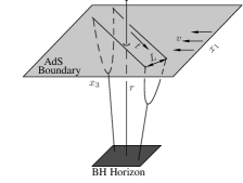
Figure 1: Left: dual configuration of the $qm$ bound state in a hot plasma wind; the dyon is described by a Y-junction of three strings of charged $(1,0)$, $(0,1)$ and $(1,1)$ with two end points attached on the AdS boundary and one end point attach on the black horizon. Right: dual configuration of the $q\bar{q}$ system in the same plasma wind; the dipole is described by a single fundamental string with both ends attached on the AdS boundary.

For comparisons, we shall also consider a $q\bar{q}$ system moving in the same plasma [13], which is simply described by a fundamental string with both ends attached on the boundary of the AdS spacetime, see the right part of Figure 1.

One may choose a frame in which the $qm$ or $q\bar{q}$ bound system is at rest. This amounts to introduce a plasma wind [13]. A hot wind in the $x^{3}$-direction can be generated by boosting the effective 5-dimensional metric (2.1) in the $(t,x^{3})$-plane

$$ds^{2}=-Adt^{2}+2Bdtdx^{3}+Cd{x^{3}}d{x^{3}}$$

$$\hskip 14.22636pt+f^{-\frac{1}{2}}(dx^{1}dx^{1}+dx^{2}dx^{2})+f^{\frac{1}{2}}h^{-1}dr^{2}$$ (2.2)

$$A=f^{-\frac{1}{2}}\gamma^{2}(h-\beta^{2}),~{}B=f^{-\frac{1}{2}}\gamma^{2}(\beta-\beta h),$$ (2.3)

$$C=f^{-\frac{1}{2}}\gamma^{2}(1-\beta^{2}h),~{}~{}\beta\equiv v,~{}\gamma\equiv 1/\sqrt{1-v^{2}}.$$

We now consider a rest dyon in the velocity-dependent background (2.2). If the separation between quark and monopole in this dyon is not along the $x^{3}$-direction, then the worldsheets of F- and D-string can be parameterized by

$$t=\tau,~{}~{}x^{1}=\sigma,~{}~{}x^{2}=\textrm{const.},~{}~{}x^{3}=x(\sigma),~{}~{}r=r(\sigma).$$ (2.4)

Accordingly, the Nambu-Goto action for F-string takes the form

$$S=-\frac{1}{2\pi\alpha^{\prime}}\int d\tau d\sigma\sqrt{-\det g_{\alpha\beta}}=-\frac{\mathcal{T}}{2\pi\alpha^{\prime}}\int d\sigma\mathcal{L}$$ (2.5)

where $\mathcal{T}$ is a large time interval and

$$\mathcal{L}=\sqrt{\gamma^{2}(h-\beta^{2})f^{-1}+hf^{-1}x^{\prime 2}+\gamma^{2}(1-\frac{\beta^{2}}{h})r^{\prime 2}}.$$ (2.6)

The action for D-string can be obtained from (2.5) by multiplying a factor of $1/g=4\pi/g_{\rm YM}^{2}$. The equation of motion derived from the lagrangian (2.6) can be integrated once with the results

$$x^{\prime 2}=\frac{p^{2}}{q^{2}}\gamma^{2}(1-\frac{\beta^{2}}{h}),~{}r^{\prime 2}=\frac{h}{f}\left[\frac{\gamma^{2}}{q^{2}}{(1-\frac{\beta^{2}}{h})(\frac{h}{f}-p^{2})-1}\right]$$ (2.7)

where $p$ and $q$ are integration constants. When $p=0$, we have $x^{\prime}(\sigma)=0$ and thus $x^{3}={\rm const.}$, this particular case describes a plasma wind blowing perpendicular to the dyon.

If the separation between quark and monopole in the dyon is along the $x^{3}$ direction, we may parameterize the F- and D-string as

$$t=\tau,~{}~{}x^{1,2}={\rm const.},~{}~{}x^{3}=\sigma,~{}~{}r=r(\sigma).$$ (2.8)

Such case corresponds to the wind blowing parallel to the dyon. With this parameterization, the lagrangian and the equation of motion read

$$\mathcal{L}=\sqrt{\frac{h}{f}+\gamma^{2}(1-\frac{\beta^{2}}{h})r^{\prime 2}},~{}~{}~{}r^{\prime 2}=\frac{h}{\gamma^{2}(h-\beta^{2})}\left[\frac{h^{2}}{q^{2}f^{2}}-\frac{h}{f}\right]$$ (2.9)

where $q$ again is an integral constant.

The $(1,1)$-string is parameterized in a somewhat different way from that of the F- and D-string.

$$t=\tau,~{}~{}~{}r=\sigma,~{}~{}~{}x^{1,2,3}=\textrm{const.}$$ (2.10)

which leads to the following Nambu-Goto action

$$\mathcal{S}=-\frac{\mathcal{T}\sqrt{1+g^{-2}}}{2\pi\alpha^{\prime}}\int_{r_{0}}^{r_{j}}dr\sqrt{\gamma^{2}(1-\beta^{2}h^{-1})},$$ (2.11)

with $r_{0}$ is the horizon of black hole and $r_{j}$ is the location of the junction point of strings.

For a $q\bar{q}$ bound state in the background (2.2) the results are similar. When the dipole is not parallel to the wind direction, the F-string connecting the quark and anti-quark can be parameterized by (2.4), so we get a lagrangian and a set of equations of motion identical to those given in (2.6) and (2.7). In the parallel case we can use the parameterization (2.8) instead, and the corresponding results are precisely the same as in (2.9).

Let us consider the plasma wind blowing perpendicular to the dyon (hence $p=0$). In such case, the first equation in (2.7) simply gives $x(\sigma)={\rm const.}$, while the second reduces to

$$r^{\prime 2}=\frac{\rho^{8}}{q^{2}}\left(\frac{r^{4}}{r_{0}^{4}}-1\right)\left(\frac{r^{4}}{r_{0}^{4}}-\gamma^{2}-\frac{q^{2}}{\rho^{4}}\right),~{}~{}~{}\rho\equiv\frac{r_{0}}{R}.$$ (2.12)

We will write $r^{\prime 2}=r^{\prime 2}[r,q]$ to emphasize the dependence of $r^{\prime 2}$ on $r$ and $q$. Now the quark and monopole in this dyon span a distance $L=L_{F}+L_{D}$ with

$$L_{F}\equiv\int_{r_{j}}^{\infty}dr\frac{1}{\sqrt{r^{\prime 2}[r,q_{F}]}},~{}~{}~{}L_{D}\equiv\int_{r_{j}}^{\infty}dr\frac{1}{\sqrt{r^{\prime 2}[r,q_{D}]}}$$ (2.13)

where $L_{F}$ and $L_{D}$ are the length of F- and D-string projected on the AdS boundary. More explicitly, one may insert (2.12) into (2.13) to write

$$L_{F,D}=\frac{r_{0}q_{F,D}}{\rho^{4}}\int_{y_{j}}^{\infty}\frac{dy}{\sqrt{(y^{4}-1)(y^{4}-\gamma^{2}-q_{F,D}^{2}/\rho^{4})}}$$ (2.14)

where $y_{j}\equiv\frac{r_{j}}{r_{0}}$ and $q_{F,D}\geq 0$. Note that the junction-point is located at outside the black hole horizon $y_{j}>1$. Thus, we must choose $y_{j}^{2}\geq\gamma^{2}+{{\rm max}\{q_{F}^{2},q_{D}^{2}\}}/\rho^{4}$ in order to make both $L_{F}$ and $L_{D}$ be real.

The integrals in (2.14) can be expressed in terms of the Appell hypergeometric $F_{1}$-function. This function, defined through the double series

$$F_{1}(a,b,b^{\prime};c;\xi,\zeta)=\sum_{m,n=0}^{\infty}\frac{(a,m+n)(b,m)(b^{\prime},n)}{(c,m+n)}\frac{\xi^{m}}{m!}\frac{\zeta^{n}}{n!},~{}~{}~{}|\xi|<1,~{}~{}|\zeta|<1$$ (2.15)

is the two-variable analogue of the ordinary Gaussian hypergeometric function $F(a,b;c;\xi)$. In some special cases we will have $F_{1}\rightarrow F$. Actually, as $\zeta\rightarrow 0$, only those terms with $n=0$ will contribute to (2.15), so in this limit $F_{1}(a,b,b^{\prime};c;\xi,0)=F(a,b;c;\xi)$. There exists a simple integral representation for (2.15)

$$F_{1}(a,b,b^{\prime};c;\xi,\zeta)=\frac{\Gamma(c)}{\Gamma(a)\Gamma(c-a)}\int_{1}^{\infty}duu^{b+b^{\prime}-c}(u-1)^{c-a-1}(u-\xi)^{-b}(u-\zeta)^{-b^{\prime}}.$$ (2.16)

clearly, for $b=b^{\prime}$ this is a symmetric function with respect to $\xi$ and $\zeta$. Another immediate consequence of (2.16) is

$$F_{1}(a,b,b^{\prime};c;\xi,1)=\frac{\Gamma(c)\Gamma(c-a-b^{\prime})}{\Gamma(c-a)\Gamma(c-b^{\prime})}F(a,b;c-b^{\prime};\xi).$$ (2.17)

To find the relation between (2.14) and (2.16), we may change the integration variable $y=y_{j}u^{1/4}$ in (2.14) and express $L_{F,D}$ as

$$L_{F,D}=\frac{r_{0}q_{F,D}}{4\rho^{4}y_{j}^{3}}\int_{1}^{\infty}duu^{-3/4}(u-1)^{0}\left(u-\frac{1}{y_{j}^{4}}\right)^{-1/2}\left(u-\frac{\gamma^{2}+q_{F,D}^{2}/\rho^{4}}{y_{j}^{4}}\right)^{-1/2}.$$ (2.18)

Comparing this with (2.16), we get $a=3/4$, $b=b^{\prime}=1/2$ and $c=7/4$. One thus obtains

$$L_{F} = \frac{r_{0}q_{F}}{3\rho^{4}y_{j}^{3}}F_{1}\left(\frac{3}{4},\frac{1}{2},\frac{1}{2};\frac{7}{4};\frac{1}{y_{j}^{4}},\frac{\gamma^{2}+q_{F}^{2}/\rho^{4}}{y_{j}^{4}}\right),$$ (2.19)

$$L_{D} = \frac{r_{0}q_{D}}{3\rho^{4}y_{j}^{3}}F_{1}\left(\frac{3}{4},\frac{1}{2},\frac{1}{2};\frac{7}{4};\frac{1}{y_{j}^{4}},\frac{\gamma^{2}+q_{D}^{2}/\rho^{4}}{y_{j}^{4}}\right).$$ (2.21)

This together with $L=L_{F}+L_{D}$ allows us to determine the distance between the quark and monopole, in terms of the location $y_{j}=r_{j}/r_{0}$ of the junction point as well as the integral constants $q_{F}$ and $q_{D}$.

Before we proceed to analyze the $qm$ system, let us pause a moment to take a look at how the Appell function behaves in the $q\bar{q}$ system. If the plasma wind blows perpendicular to the dipole, the distance $L$ between $q$ and $\bar{q}$ can be similarly expressed by

$$L=2\int_{r_{j}}^{\infty}dr\frac{1}{\sqrt{r^{\prime 2}[r,q]}}$$ (2.22)

(2.23)

$$\hskip 14.22636pt=\frac{2r_{0}q}{3\rho^{4}y_{j}^{3}}F_{1}\left(\frac{3}{4},\frac{1}{2},\frac{1}{2};\frac{7}{4};\frac{1}{y_{j}^{4}},\frac{\gamma^{2}+q^{2}/\rho^{4}}{y_{j}^{4}}\right).$$ (2.24)

One simplicity in the $q\bar{q}$ system is the location of junction point $r_{j}$ is actually the middle point of a single smooth string. When it passed through this point along the string, the value of $r^{\prime}$ changes a sign $r^{\prime}\rightarrow-r^{\prime}$ but does not jump, which implying $r^{\prime}[r_{j},q]=0$. Combining this smoothness condition with (2.12) and the fact that $r_{j}>r_{0}$, we see that the location of the junction point is completely determined, given by $y_{j}^{4}=\gamma^{2}+q^{2}/\rho^{4}$. Thus, the equation (2.24) reduces to

$$L=\frac{(2\pi)^{3/2}}{\Gamma(1/4)^{2}}\frac{r_{0}}{\rho^{2}}\frac{q/\rho^{2}}{(\gamma^{2}+q^{2}/\rho^{4})^{3/4}}F\left(\frac{3}{4},\frac{1}{2};\frac{5}{4};\frac{1}{\gamma^{2}+q^{2}/\rho^{4}}\right),$$ (2.25)

here we have applied the formula (2.17). Now for a fixed boost factor $\gamma$ and considering the asymptotic behavior of $L$ at $q\approx 0$ and $q\approx\infty$, the result can be directly read off from (2.25). For a small $q$, we have $L\propto q\sim 0$, while for a large $q$, $L\propto 1/\sqrt{q}\sim 0$. So $L$ must have a maximal value $L_{\rm max}$ at some $q=q_{m}$, and this gives the screen length $L_{s}=L_{\rm max}$. To see the velocity dependence of $L_{s}$ analytically, we have to take the ultra-relativistic limit $\gamma\rightarrow\infty$, under which the hypergeometric function in (2.25) behaves as $F=1+\mathcal{O}((\gamma^{2}+q^{2}/\rho^{4})^{-1})$. So at the leading order we have $L\propto q(\gamma^{2}+q^{2}/\rho^{4})^{-3/4}$, which implying $q_{m}=\sqrt{2}\gamma\rho^{2}$ and therefore we get

$$L_{s}=\frac{r_{0}}{\rho^{2}}f_{q\bar{q}}(1-v^{2})^{1/4},~{}~{}~{}~{}f_{q\bar{q}}\approx\frac{4\pi^{3/2}}{3^{3/4}\Gamma(1/4)^{2}}.$$ (2.26)

The numerical result of [13] shows that (2.26) holds even beyond the ultra-relativistic limit, with $f_{q\bar{q}}=f_{q\bar{q}}(v)$ being now a function mildly depending on $v$.

Returning to the quark-monopole system, we notice that in general it is not possible to impose the smoothness condition at the Y-junction point $r_{j}$, and in particular $r^{\prime}$ may have a jump when going from F-string to D-string. The correct condition to determine $y_{j}$ is that the net force at the string junction should vanish [17] (otherwise the junction point would move away to lower the energy). Recall that the force exerted by a string at some point is described by $F^{I}=\hat{T}E^{I}_{A}dx^{A}/ds$, where $\hat{T}$ denotes the effective string tension at that point, and $E^{I}_{A}$ is a set of vierbeins associated to the spacetime metric $ds^{2}=G_{AB}dx^{A}dx^{B}$. The tension $\hat{T}$ measures energy per unit length along the string, hence $\hat{T}ds=(2\pi\alpha^{\prime})^{-1}\mathcal{L}d\sigma$. We will now evaluate $F^{I}$ at the Y-junction point exerted by each string. So we set $T_{(1,0)}$, $T_{(0,1)}$ and $T_{(1,1)}$ to be the tensions of the F-, D- and $(1,1)$-string, respectively, at $r=r_{j}$. For the F-string we have $x_{1}=\sigma$ and $r=r(\sigma)$, where $r$ is the solution of (2.12) with $q=q_{F}$. The infinitesimal length along this string is given by

$$ds^{2}=(f^{-1/2}+f^{1/2}h^{-1}r^{\prime 2})d\sigma^{2}=\frac{\rho^{6}y_{j}^{2}(y_{j}^{4}-\gamma^{2})}{q_{F}^{2}}d\sigma^{2}.$$ (2.27)

On the other hand, the Lagrangian (2.6) with $x_{3}^{\prime}=0$ can be evaluated as

$$\mathcal{L}=\gamma f^{-1/4}(h-\beta^{2})^{1/2}(f^{-1/2}+f^{1/2}h^{-1}r^{\prime 2})^{1/2}$$ (2.28)

$$=\gamma f^{-1/4}(h-\beta^{2})^{1/2}\frac{ds}{d\sigma},$$ (2.29)

from which one immediately get

$$T_{(1,0)}=\frac{\gamma f^{-1/4}}{2\pi\alpha^{\prime}}\sqrt{h-\beta^{2}}=\frac{\rho}{2\pi\alpha^{\prime}y_{j}}\sqrt{y_{j}^{4}-\gamma^{2}}.$$ (2.30)

Thus, the force $\vec{F}_{(1,0)}$ exerted by the F-string at $r=r_{j}$ has two non-vanishing components, which are determined by

$$F^{1}_{(1,0)}=T_{(1,0)}f^{-1/4}\frac{dx^{1}}{ds}=-\frac{q_{F}}{2\pi\alpha^{\prime}\rho y_{j}},$$ (2.31)

(2.32)

$$F^{r}_{(1,0)}=T_{(1,0)}f^{1/4}h^{-1/2}\frac{dr}{ds}=\frac{\rho}{2\pi\alpha^{\prime}y_{j}}\sqrt{y_{j}^{4}-\gamma^{2}-q_{F}^{2}/\rho^{4}}.$$ (2.33)

A similar computation applies to the D- and $(1,1)$-string. It is easy to derive, for example, $T_{(0,1)}=T_{(1,0)}/g$, $T_{(1,1)}=T_{(1,0)}\sqrt{1+g^{-2}}$. The final result of $\vec{F}_{(0,1)}$ and $\vec{F}_{(1,1)}$ reads

$$F^{1}_{(0,1)}=\frac{q_{D}}{2\pi\alpha^{\prime}\rho y_{j}g},~{}~{}~{}F^{r}_{(0,1)}=\frac{\rho}{2\pi\alpha^{\prime}y_{j}g}\sqrt{y_{j}^{4}-\gamma^{2}-q_{D}^{2}/\rho^{4}},$$ (2.34)

(2.35)

$$F^{1}_{(1,1)}=0,~{}~{}~{}~{}~{}F^{r}_{(1,1)}=-\frac{\rho\sqrt{1+g^{-2}}}{2\pi\alpha^{\prime}y_{j}}\sqrt{y_{j}^{4}-\gamma^{2}}.$$ (2.36)

Having found these forces, we are now ready to impose the condition $\vec{F}_{(1,0)}+\vec{F}_{(0,1)}+\vec{F}_{(1,1)}=0$. The $x^{1}$-component of this condition gives a simple relation between $q_{F}$ and $q_{D}$, while the $r$-component can be used to determine $y_{j}$ in terms of $q_{F}$ and $q_{D}$. Explicitly, we have

$$q_{D}=gq_{F},~{}~{}~{}y_{j}^{4}=\gamma^{2}+(1+g^{2})\frac{q_{F}^{2}}{\rho^{4}}=\gamma^{2}+\frac{q_{F}^{2}+q_{D}^{2}}{\rho^{4}}.$$ (2.37)

Thus, the expression for $y_{j}^{4}$ looks quite similar to that in the $q\bar{q}$ system. It is interesting to note that the location of the junction point does not change under the S-duality transformation $g\leftrightarrow 1/g$ and $q_{F}\leftrightarrow q_{D}$.

One can use the equation (2.37) to eliminate the dependence of $L$ on $y_{j}$ and $q_{D}$, and express this distance as a single-variable function in $q_{F}\equiv q$. The screening effect can be analyzed by looking at the maximal value of $L=L(q)$ at some $q=q_{m}$, in analog to the $q\bar{q}$ case [13]. After substituting (2.37) into (2.21), we obtain

$$L=\frac{r_{0}}{3\rho^{2}}\frac{q/\rho^{2}}{[\gamma^{2}+(1+g^{2})q^{2}/\rho^{4}]^{3/4}}\cdot$$ (2.38)

(2.39)

$$\left[F_{1}\left(\frac{3}{4},\frac{1}{2},\frac{1}{2};\frac{7}{4};\frac{1}{\gamma^{2}+(1+g^{2})q^{2}/\rho^{4}},\frac{\gamma^{2}+q^{2}/\rho^{4}}{\gamma^{2}+(1+g^{2})q^{2}/\rho^{4}}\right)\right.$$ (2.40)

(2.41)

$$+\left.gF_{1}\left(\frac{3}{4},\frac{1}{2},\frac{1}{2};\frac{7}{4};\frac{1}{\gamma^{2}+(1+g^{2})q^{2}/\rho^{4}},\frac{\gamma^{2}+g^{2}q^{2}/\rho^{4}}{\gamma^{2}+(1+g^{2})q^{2}/\rho^{4}}\right)\right].$$

One may fix the boost factor $\gamma$ and examine the asymptotic behavior of $L$ in the small and large $q$ regions, as in the $q\bar{q}$ case. When $q\rightarrow 0$, the two $F_{1}$ functions in (2.40) behave smoothly, both approaching to the $\gamma$-dependent constant

$$F_{1}\left(\frac{3}{4},\frac{1}{2},\frac{1}{2};\frac{7}{4};\frac{1}{\gamma^{2}},1\right)=\frac{3(2\pi)^{3/2}}{2\Gamma(1/4)^{2}}F\left(\frac{3}{4},\frac{1}{2};\frac{5}{4};\frac{1}{\gamma^{2}}\right)$$ (2.42)

where we have used the formula (2.17). So we find $L\propto q\rightarrow 0$ in this limit. Similarly we see that in the limit $q\rightarrow\infty$, then $L\propto 1/\sqrt{q}\rightarrow 0$. Thus, $L=L(q)$ is a function positive everywhere, it must have a maximal value $L_{\rm max}$ at some extremal point $q=q_{m}$. For convenience, we define a dimensionless quantity $\pi TL$. Then, through some numerical calculations, we show $\pi TL$ (at fixed temperature) to depend on the parameter $q/\rho^{2}$ at fixed coupling constant $g$ and velocity $v$ in Fig. 2 and Fig. 3.

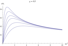
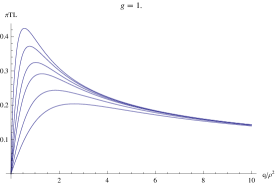
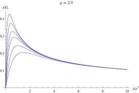
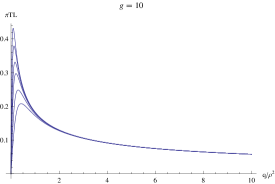
Figure 2: Plots of $l\equiv\rho^{2}L/r_{0}=\pi TL$ as a function of $q/\rho^{2}$ at $g=0.5,~{}1.0,~{}2.5$ and $10$, respectively, for $v=0,~{}0.5,~{}0.7,~{}0.8,~{}0.9,~{}0.95$ (top to bottom).

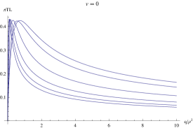
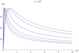
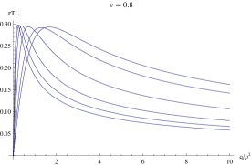
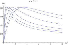
Figure 3: Plots of $l\equiv\rho^{2}L/r_{0}=\pi TL$ as a function of $q/\rho^{2}$ at $v=0,~{}0.5,~{}0.8$ and $0.95$, respectively, for $g=0.5,~{}1.0,~{}2.5,~{}5.0,~{}7.5,~{}10$ (right to left).

These two figures indicate that the quark-monopole system indeed has a screening length $L_{s}=L_{max}$. In addition, we find that (i) the screening length $L_{s}$ of the $qm$ system is smaller than that of the $q\bar{q}$ pair, and (ii) in the $qm$ case, the dependence of $L_{s}$ on the coupling constant $g$ is rather mild. In order to show the dependence of $L_{s}$ on $(1-v^{2})^{1/4}$, we define $f(v,g)\equiv(1-v^{2})^{-1/4}\pi TL_{s}$. Then, the dependence of $f(v,g)$ on the parameters $v$ and $g$ is plotted in Fig. 4.

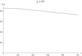
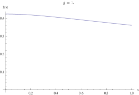
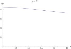
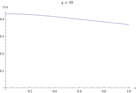
Figure 4: The dependence of $f(v,g)$ on $v$ for $g=0.5,~{}1.0,~{}2.5,~{}10$ is respectively plotted.

It shows that this dependence on the parameter $g$ is mild, and its dependence on $v$ is similar to the $q\bar{q}$ case. This provides an explicit test of the prediction mentioned in the introduction: $(1-v^{2})^{1/4}$ is a kind of ”kinetic” factor that can be seen in any bound systems in the $\mathcal{N}=4$ hot plasma.

It is possible to derive the ultra-relativistic behavior of the screening length analytically. Let us take the large $\gamma$ limit and approximate the equation (2.40) by

$$L=\frac{r_{0}}{3\rho^{2}}\frac{q/\rho^{2}}{[\gamma^{2}+(1+g^{2})q^{2}/\rho^{4}]^{3/4}}\cdot$$ (2.43)

(2.44)

$$\left[F\left(\frac{3}{4},\frac{1}{2};\frac{7}{4};\frac{\gamma^{2}+q^{2}/\rho^{4}}{\gamma^{2}+(1+g^{2})q^{2}/\rho^{4}}\right)\right.$$ (2.45)

(2.46)

$$+\left.gF\left(\frac{3}{4},\frac{1}{2};\frac{7}{4};\frac{\gamma^{2}+g^{2}q^{2}/\rho^{4}}{\gamma^{2}+(1+g^{2})q^{2}/\rho^{4}}\right)\right].$$

One may consider a range of $q$ behaves as $q\sim\gamma^{\alpha}u$ with some fixed number $\alpha$ and a rescaled variable $u\sim\mathcal{O}(\gamma^{0})$. It is not difficult to see that such a range does not contain the extremal point $q_{m}$ of $L$, unless $\alpha=1$. In fact, if $\alpha\neq 1$, each hypergeometric function in (2.45) will tend to a constant be independent of $u$ in the limit $\gamma\rightarrow\infty$, so that $L$ can be further approximated by

$$L(q)\propto\frac{q/\rho^{2}}{[\gamma^{2}+(1+g^{2})q^{2}/\rho^{4}]^{3/4}}$$ (2.47)

(2.48)

$$\hskip 14.22636pt\Longrightarrow L^{\prime}(q)\propto\frac{2\gamma^{2}-(1+g^{2})q^{2}/\rho^{4}}{[\gamma^{2}+(1+g^{2})q^{2}/\rho^{4}]^{7/4}}.$$ (2.49)

It follows that $L^{\prime}(q)$ never vanishes in that range. Thus, the extremal point $q_{m}$ has to scale as $q_{m}=\gamma u_{m}$ with $u_{m}\sim{\mathcal{O}}(\gamma^{0})$. Substituting this into (2.45) we obtain the scaling behavior of the screening length $L_{s}=L(q_{m})\sim(1-v^{2})^{1/4}$ in the large $\gamma$ regime.

3 Summaries

We consider a quark-monopole system through using its gravity dual description. In the gravity side, this configuration includes F-string, D-string and $(1,1)$-string, which are connected at a junction point. We calculate the screening length of quark-monopole bound state moving in a hot $\mathcal{N}=4$ SYM plasma. We find the screening length $L_{s}$ is smaller than that of the quark-antiquark bound state. And its dominant dependence of $L_{s}$ on the wind velocity $v$ is proportional to $(1-v^{2})^{1/4}$. Finally, the dependence of screening length $L_{s}$ on the string coupling constant $g$ is very mild. Thus, it is not very easy to distinguish the quark-antiquark pair from the quark-monopole bound state through calculating the screening length in a hot plasma.

Acknowledgments

We are very glad to thank Prof. Yi-hong Gao for the collaboration in the early stage of this project. The work of W.-s. Xu is partly supported by K. C. Wong Magna Fund in Ningbo University, National Science Foundation of China under Grant No. 11205093 and 11347020. The work of D.-f. Zeng is surpported by BJNSF under Grant No. 1102007.

Appendix A Quark-monopole potential

In this appendix, we should investigate the quark-monopole potential in the $AdS_{5}\times S^{5}$ black hole background (2.1). Similar computation of this binding potential also is performed in [18]. We assume the worldsheets of F- and D-string are parameterized by $\tau=t$ and $\sigma=x^{1}$, then the action for F-string is

$$S=\frac{1}{2\pi\alpha^{\prime}}\int d\tau d\sigma\sqrt{r^{\prime 2}+\frac{h}{f}},$$ (A.1)

which can be derived from the equation (2.6) by setting the velocity of plasma wind $v=0$. The action for D-string is got by multiplying the factor $1/g$ on the action of F-string. Then the equation of motion reads

$$r^{\prime 2}=\frac{h^{2}}{q_{F,D}^{2}f^{2}}-\frac{h}{f}$$ (A.2)

with the integral constants $q_{F}$ and $q_{D}$ for F- and D-string respectively. From the equation (2.14), the lengths of F- and D-string are

$$L_{F,D}=\int_{r_{j}}^{\infty}\frac{dr}{\sqrt{\frac{h^{2}}{q_{F,D}^{2}f^{2}}-\frac{h}{f}}}=\frac{r_{0}q_{F,D}}{\rho^{4}}\int_{y_{j}}^{\infty}\frac{dy}{\sqrt{(y^{4}-1)(y^{4}-1-q_{F,D}^{2}/\rho^{4})}},$$ (A.3)

where $y_{j}=r_{j}/r_{0}$, and $r_{j}$ is the junction point of F-, D- and $(1,1)$-string. Thus, the distance between quark and monopole in the dyon is

$$L=\frac{r_{0}}{3\rho^{2}}\frac{q_{F}/\rho^{2}}{[1+(q_{F}^{2}+q_{D}^{2})/\rho^{4}]^{3/4}}\cdot$$ (A.4)

(A.5)

$$\left[F_{1}\left(\frac{3}{4},\frac{1}{2},\frac{1}{2};\frac{7}{4};\frac{1}{1+(q_{F}^{2}+q_{D}^{2})/\rho^{4}},\frac{1+q_{F}^{2}/\rho^{4}}{1+(q_{F}^{2}+q_{D}^{2})/\rho^{4}}\right)\right.$$ (A.6)

(A.7)

$$+\left.gF_{1}\left(\frac{3}{4},\frac{1}{2},\frac{1}{2};\frac{7}{4};\frac{1}{1+(q_{F}^{2}+q_{D}^{2})/\rho^{4}},\frac{1+q_{D}^{2}/\rho^{4}}{1+(q_{F}^{2}+q_{D}^{2})q^{2}/\rho^{4}}\right)\right].$$

By using the equation (A.1) and subtracting the divergence, the potential of quark-monopole is expressed as

$$E_{QM}=\frac{r_{0}}{2\pi\alpha^{\prime}}\left[\int_{y_{j}}^{\infty}dy\left(\frac{1}{\sqrt{1-q_{F}^{2}\frac{f}{h}}}-1\right)-(y_{j}-1)\right.$$ (A.8)

$$\left.+\frac{1}{g}\int_{y_{j}}^{\infty}dy\left(\frac{1}{\sqrt{1-q_{D}^{2}\frac{f}{h}}}-1\right)-(y_{j}-1)/g+\sqrt{1+g^{-2}}~{}(y_{j}-1)\right].$$ (A.9)

If $r_{0}=0$, then the distance $L$ and potential $E_{QM}$ will reduce to the corresponding cases [17]. By using the equations (A.6) and (A.9), and the vanishing condition of net force

$$q_{D}=gq_{F},~{}~{}y_{j}^{4}=1+\frac{q_{F}^{2}+q_{D}^{2}}{\rho^{4}}$$ (A.10)

at junction point of F-, D- and (1, 1)-string, the quark-monopole potential at finite temperature reads

$$E_{QM}=\frac{\sqrt{4\pi N}}{6\pi L}\,\sqrt{g}\,\frac{q_{F}/\rho^{2}}{[1+(q_{F}^{2}+q_{D}^{2})/\rho^{4}]^{3/4}}\cdot$$ (A.11)

(A.12)

$$\left[F_{1}\left(\frac{3}{4},\frac{1}{2},\frac{1}{2};\frac{7}{4};\frac{1}{1+(q_{F}^{2}+q_{D}^{2})/\rho^{4}},\frac{1+q_{F}^{2}/\rho^{4}}{1+(q_{F}^{2}+q_{D}^{2})/\rho^{4}}\right)\right.$$ (A.13)

(A.14)

$$\hskip 11.38109pt+\left.gF_{1}\left(\frac{3}{4},\frac{1}{2},\frac{1}{2};\frac{7}{4};\frac{1}{1+(q_{F}^{2}+q_{D}^{2})/\rho^{4}},\frac{1+q_{D}^{2}/\rho^{4}}{1+(q_{F}^{2}+q_{D}^{2})/\rho^{4}}\right)\right]\cdot$$ (A.15)

$$\left[\int_{y_{j}}^{\infty}dy\left(\frac{1}{\sqrt{1-q_{F}^{2}\frac{f}{h}}}-1\right)-(y_{j}-1)\right.$$ (A.16)

$$\left.\hskip 8.53581pt+\frac{1}{g}\int_{y_{j}}^{\infty}dy\left(\frac{1}{\sqrt{1-q_{D}^{2}\frac{f}{h}}}-1\right)-(y_{j}-1)/g+\sqrt{1+g^{-2}}~{}(y_{j}-1)\right].$$ (A.17)

This potential is negative for all coupling constant $g$, which is shown by the left figure of Fig. 5. We also plot the dependence of this binding energy on the temperature in the right figure of Fig. 5.

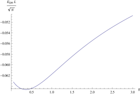
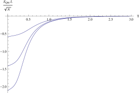
Figure 5: The dependence of $\frac{E_{QM}L}{\sqrt{N}}$ on $g$ is plotted with $R=1$, $q_{F}=1$ and $\rho=10$ on the left. For the right figure, it shows $\frac{E_{QM}L}{\sqrt{N}}$ depends on the temperature $T$ at $g=0.5,~{}1,~{}2.5$ from bottom to up with setting $R=1$ and $q_{F}=1$.

As expected, the binding energy of quark-monopole will approach to zero as the junction point $r_{j}$ goes to the horizon of black hole. The reason is now the junction point will pass through the horizon, and the F- and D-sting will be not connected. From the equation (2.37), we know the junction point $y_{j}$ is invariant under the S-duality transformation $g\leftrightarrow 1/g$ and $q_{F}\leftrightarrow q_{D}$. Thus, the quark-monopole potential at finite temperature is still invariant under the S-duality. Similar to the cases of $q\bar{q}$ and $qm$ at zero temperature, the potential is still proportional to $1/L$ even if the conformal symmetry is broken by the temperature of black hole.

References

• [1] J. M. Maldacena, “The large N limit of superconformal field theories and supergravity,” Adv. Theor. Math. Phys.  2, 231 (1998) [Int. J. Theor. Phys.  38, 1113 (1999)]; S. S. Gubser, I. R. Klebanov and A. M. Polyakov, “Gauge theory correlators from non-critical string theory,” Phys. Lett.  B 428, 105 (1998) [arXiv:hep-th/9802109]; E. Witten, “Anti-de Sitter space and holography,” Adv. Theor. Math. Phys.  2, 253 (1998) [arXiv:hep-th/9802150]; E. Witten, “Anti-de Sitter space, thermal phase transition, and confinement in gauge theories,” Adv. Theor. Math. Phys.  2, 505 (1998) [arXiv:hep-th/9803131].
• [2] G. Policastro, D. T. Son and A. O. Starinets, “The Shear viscosity of strongly coupled N=4 supersymmetric Yang-Mills plasma,” Phys. Rev. Lett.  87, 081601 (2001) [hep-th/0104066].
• [3] P. Kovtun, D. T. Son and A. O. Starinets, “Holography and hydrodynamics: Diffusion on stretched horizons,” JHEP 0310 (2003) 064 [arXiv:hep-th/0309213].
• [4] A. Buchel and J. T. Liu, “Universality of the shear viscosity in supergravity,” Phys. Rev. Lett.  93, 090602 (2004) [arXiv:hep-th/0311175].
• [5] P. Kovtun, D. T. Son and A. O. Starinets, “Viscosity in strongly interacting quantum field theories from black hole physics,” Phys. Rev. Lett.  94, 111601 (2005) [arXiv:hep-th/0405231].
• [6] J. Mas, “Shear viscosity from R-charged AdS black holes,” JHEP 0603, 016 (2006) [hep-th/0601144].
• [7] M. Brigante, H. Liu, R. C. Myers, S. Shenker and S. Yaida, “Viscosity Bound Violation in Higher Derivative Gravity,” Phys. Rev. D 77, 126006 (2008) [arXiv:0712.0805 [hep-th]].
• [8] M. Brigante, H. Liu, R. C. Myers, S. Shenker and S. Yaida, “The Viscosity Bound and Causality Violation,” Phys. Rev. Lett.  100, 191601 (2008) [arXiv:0802.3318 [hep-th]].
• [9] A. Rebhan and D. Steineder, “Violation of the Holographic Viscosity Bound in a Strongly Coupled Anisotropic Plasma,” Phys. Rev. Lett.  108, 021601 (2012) [arXiv:1110.6825 [hep-th]].
• [10] H. Liu, K. Rajagopal and U. A. Wiedemann, “Calculating the jet quenching parameter from AdS/CFT,” Phys. Rev. Lett.  97, 182301 (2006) [hep-ph/0605178].
• [11] C. P. Herzog, A. Karch, P. Kovtun, C. Kozcaz and L. G. Yaffe, “Energy loss of a heavy quark moving through N=4 supersymmetric Yang-Mills plasma,” JHEP 0607, 013 (2006) [hep-th/0605158]; S. S. Gubser, “Drag force in AdS/CFT,” Phys. Rev. D 74, 126005 (2006); [hep-th/0605182]; J. Casalderrey-Solana and D. Teaney, “Heavy quark diffusion in strongly coupled N = 4 Yang Mills,” Phys. Rev.  D 74, 085012 (2006) [arXiv:hep-ph/0605199].
• [12] B. Alessandro et al. [NA50 Collaboration], “A New measurement of J/psi suppression in Pb-Pb collisions at 158-GeV per nucleon,” Eur. Phys. J. C 39, 335 (2005) [hep-ex/0412036].
• [13] H. Liu, K. Rajagopal and U. A. Wiedemann, “An AdS/CFT Calculation of Screening in a Hot Wind,” Phys. Rev. Lett.  98, 182301 (2007) [hep-ph/0607062].
• [14] M. Chernicoff, J. A. Garcia and A. Guijosa, “The Energy of a Moving Quark-Antiquark Pair in an N=4 SYM Plasma,” JHEP 0609, 068 (2006) [hep-th/0607089].
• [15] E. Caceres, M. Natsuume and T. Okamura, “Screening length in plasma winds,” JHEP 0610, 011 (2006) [hep-th/0607233].
• [16] J. Casalderrey-Solana, H. Liu, D. Mateos, K. Rajagopal and U. A. Wiedemann, “Gauge/String Duality, Hot QCD and Heavy Ion Collisions,” arXiv:1101.0618 [hep-th].
• [17] J. A. Minahan, “Quark - monopole potentials in large N superYang-Mills,” Adv. Theor. Math. Phys.  2, 559 (1998) [hep-th/9803111].
• [18] K. Sfetsos and K. Siampos, “String junctions in curved backgrounds, their stability and dyon interactions in SYM,” Nucl. Phys. B 797, 268 (2008) [arXiv:0710.3162 [hep-th]].