On the accretion properties of young stellar objects in the L1615/L1616 cometary cloud

We present the results of FLAMES/UVES and FLAMES/GIRAFFE spectroscopic observations of 23 low-mass stars in the L1615/L1616 cometary cloud, complemented with FORS2 and VIMOS spectroscopy of 31 additional stars in the same cloud. L1615/L1616 is a cometary cloud where the star formation was triggered by the impact of the massive stars in the Orion OB association. From the measurements of the lithium abundance and radial velocity, we confirm the membership of our sample to the cloud. We use the equivalent widths of the H$\alpha$, H$\beta$, and the He i $\lambda$5876, $\lambda$6678, $\lambda$7065 Å emission lines to calculate the accretion luminosities, $L_{\rm acc}$, and the mass accretion rates, $\dot{M}_{\rm acc}$. We find in L1615/L1616 a fraction of accreting objects ($\sim 30\%$), which is consistent with the typical fraction of accretors in T associations of similar age ($\sim 3$ Myr). The mass accretion rate for these stars shows a trend with the mass of the central object similar to that found for other star-forming regions, with a spread at a given mass which depends on the evolutionary model used to derive the stellar mass. Moreover, the behavior of the $2MASS/WISE$ colors with $\dot{M}_{\rm acc}$ indicates that strong accretors with $\log\dot{M}_{\rm acc}\raisebox{-2.15277pt}{$\>\stackrel{{\scriptstyle\textstyle>}}{{\sim}}\>$}-8.5$ dex show large excesses in the $JHK{\rm s}$ bands, as in previous studies. We also conclude that the accretion properties of the L1615/L1616 members are similar to those of young stellar objects in T associations, like Lupus.

1 Introduction

The Lynds 1616 cloud (hereafter L1616; Lynds 1962), at a distance of about 450 pc, forms, together with Lynds 1615 (hereafter L1615), a cometary-shaped cloud west of the Orion OB association ($\alpha\sim 5^{\rm h}7^{\rm m}$, $\delta\sim-3{\degr}20^{\prime}$; see review by Alcalá et al. 2008, and references therein). It extends about $40^{\prime}$ in the sky and shows evidence of ongoing star formation activity that might have been triggered by the ultraviolet (UV) radiation coming from the massive stars in the Orion OB association (see Stanke et al. 2002, and references therein). In particular, recent studies led by Lee & Chen (2007) support the validity of the radiation-driven implosion mechanism, where the UV photons from luminous massive stars create expanding ionization fronts to evaporate and compress nearby clouds into bright-rimmed or comet-shaped clouds, like L1615/L1616. Implosive pressure then causes dense clumps to collapse, prompting the formation of stars. Young stars in comet-shaped clouds are therefore likely to have been formed by a triggering mechanism.

Alcalá et al. (2004) reported a sample of 33 young stellar objects (YSOs) associated with L1615/L1616, while Gandolfi et al. (2008) performed a comprehensive census of the pre-main sequence (PMS) population in L1615/L1616, which consists of 56 YSOs. These two works were focused on the investigation of the star formation history, the relevance of the triggered scenario, and the initial mass function, but no study on accretion properties was addressed. As a continuation of these works, here we use further spectroscopic observations to derive the accretion luminosity, $L_{\rm acc}$, and the mass accretion rate, $\dot{M}_{\rm acc}$, of a sample of low-mass YSOs in L1615/L1616. We also investigate whether the accretion properties of young stellar objects in a cometary cloud like L1615/L1616 are similar to those of PMS stars in T associations, like Lupus, Taurus or Chamaeleon.

The outline of the paper is as follows. In Sect. 2, we describe the spectroscopic observations, the data reduction, and the sample investigated. In Sect. 3, several accretion diagnostics are used to derive the mass accretion rates. The main results on the accretion and infrared (IR) properties are discussed in Sect. 4, while our conclusions are presented in Sect. 5.

2 Observations, data reduction, and the sample

2.1 FLAMES observations and data reduction

The observations were conducted in February-March 2006 in visitor mode using FLAMES (UVES+GIRAFFE) at the VLT. The CD#3 cross-disperser and the LR6 grating were used for the UVES and GIRAFFE spectrographs, respectively. A brief summary of the observations is given in Table 1, while the complete journal of the observations is given in Table On the accretion properties of young stellar objects in the L1615/L1616 cometary cloud. We observed 23 low-mass ($0.1\raisebox{-2.15277pt}{$\>\stackrel{{\scriptstyle\textstyle<}}{{\sim}}\>$}M_{\star}\raisebox{-2.15277pt}{$\>\stackrel{{\scriptstyle\textstyle<}}{{\sim}}\>$}2.3M_{\odot}$) objects with GIRAFFE in the MEDUSA mode; one target (the classical T Tauri star - CTTs - LkH$\alpha$ 333) was observed with both spectrographs. Nineteen objects were observed several (2–7) times within 2 days (see Table On the accretion properties of young stellar objects in the L1615/L1616 cometary cloud).

The reduction of the UVES spectra was performed using the pipeline developed by Modigliani et al. (2004), which includes the following steps: subtraction of a master bias, échelle order definition, extraction of thorium-argon spectra, normalization of a master flat-field, frame extraction, wavelength calibration, and correction of the science frame for the normalized master flat-field. Sky subtraction was performed with the IRAF task sarith using the fibers allocated to the sky.

The GIRAFFE data were reduced using the GIRAFFE Base-Line Data Reduction Software 1.13.1 (girBLDRS; Blecha et al. 2000): bias and flat-field subtraction, correction for the fiber transmission coefficient, wavelength calibration, and science frame extraction were performed. Then, a sky correction was applied to each stellar spectrum using the task sarith in the IRAF echelle package and by subtracting the average of several sky spectra obtained simultaneously during a given night.

Table 1: Summary of the observations.

Instrument	Range	Resolution	# stars	# spectra
	(Å)	($\lambda/\Delta\lambda$)
UVES	4764–6820	47 000	1	6
GIRAFFE	6438–7184	8 600	23	53

2.2 The sample

Since our goal is to investigate the accretion and the IR properties of the YSOs in the cometary cloud, we need a well characterized sample of YSOs both in terms of their physical parameters and their association with the cloud, as well as in terms of their accretion diagnostics and IR colors.

The stellar parameters (spectral types, effective temperatures, luminosities, and masses) were derived by Gandolfi et al. (2008). We adopt those determinations here. We note that one object, namely TTS 050730.9$-$031846, has a significantly lower luminosity compared to the other objects in the sample (see Fig. 3 in Gandolfi et al. 2008). This most-probable sub-luminous object is further discussed in Appendix C.

Regarding the association with the cloud, we investigated the kinematics by means of radial velocity (RV) determinations, $V_{\rm rad}$, and lithium abundance, $\log n{\rm(Li)}$, following the same methods as in Biazzo et al. (2012). The details of such determinations can be found in Appendix A.1. The radial velocity distribution of the YSOs in L1615/L1616 has an average of $\langle V_{\rm rad}\rangle=23.2\pm 3.1$ km s^-1 (see Fig. 9), which is consistent with that reported by Alcalá et al. (2004) (i.e. $\langle V_{\rm rad}\rangle=22.3\pm 4.6$ km s^-1), and in general with that of the Orion complex (see, e.g., Briceño 2008; Biazzo et al. 2009; Sergison et al. 2013). Likewise, the average lithium abundance is $\log n{\rm(Li)}$ $\sim 3.3$ dex with a dispersion of $\pm 0.3$ dex (see Table On the accretion properties of young stellar objects in the L1615/L1616 cometary cloud and Appendix A.2). Both radial velocities and lithium abundances confirm that all targets studied in this work are associated with the cometary cloud.

In order to have a more complete sample, we included in our analysis the YSOs lacking FLAMES spectroscopy, but for which Gandolfi et al. (2008) have provided measurements of the H$\alpha$ equivalent width from FORS2@VLT and VIMOS@VLT low-resolution spectra acquired in February-March 2003. Figure 1 shows the comparison between our H$\alpha$ equivalent widths ($EW_{\rm H\alpha}$) and the measurements reported by Gandolfi et al. (2008) for the stars in common. Although there is a general agreement, the Gandolfi et al. (2008) $EW_{\rm H\alpha}$ are systematically higher than ours in average by about 4 Å (excluding the three most deviating stars). We believe that this systematic difference is due to the lower spectral resolution used by Gandolfi et al. (2008) with respect to the resolution of our FLAMES spectra, whereas for the three YSOs that deviate significantly from the 1:1 relationship in Fig. 1 the differences are most likely related to variability. Two of these objects will result to be accretors (see later on) and their variability will be discussed in Sections C.1 and C.3, while the other is a weak lined T Tauri star (WTTs) and the difference of $\sim 10$ Å between our $EW_{\rm H\alpha}$ and the values by Gandolfi et al. (2008) could be related to stellar activity phenomena. This comparison justifies in the following analysis the use of the Gandolfi et al. (2008) $EW_{\rm H\alpha}$ values for the stars not observed by us. Therefore, our analysis is based on 23 objects observed by us with FLAMES, and 31 targets previously observed by Gandolfi et al. (2008) at low resolution. All these objects are listed in Tables On the accretion properties of young stellar objects in the L1615/L1616 cometary cloud and On the accretion properties of young stellar objects in the L1615/L1616 cometary cloud.

We used the criteria of White & Basri (2003) based on spectral types and $EW_{\rm H\alpha}$ to distinguish between accretors and non-accretors. In this way, a total of 15 YSOs in L1615/L1616 can be classified as accretors, 7 within our sample and 8 within the Gandolfi et al. (2008) sample. Note that TTS 050649.8$-$031933, originally classified as a WTTs by Gandolfi et al. (2008) is tagged here as accretor because its spectrum shows helium and forbidden oxygen lines in emission (see Sect. C.2), typical of accreting objects (see their Table 4).

In addition, we considered ancillary IR data both from the Two-Micron All Sky Survey ($2MASS$; Cutri et al. 2003) and from the Wide-field Infrared Survey Explorer ($WISE$; Cutri et al. 2012) catalogues (see Table On the accretion properties of young stellar objects in the L1615/L1616 cometary cloud) to investigate the IR properties of the sample and their possible correlation with accretion diagnostics.

The position in the $2MASS$ color-color diagram of all YSOs classified here as accretors and non-accretors is shown in Fig. 2 (filled and opened symbols, respectively). All YSOs classified by us as accretors show near-IR excess. The anomalous colors of TTS 050730.9$-$031846 are consistent with its sub-luminous nature (see Section C.1). The three non-accretors with apparently infrared excess represent stars with high values of $A_{V}$, as reported by Gandolfi et al. (2008). Their $WISE$ colors are typical of Class III objects, confirming their WTTs nature (see Fig. 3). Moreover, note that all YSOs classified here as accretors have $WISE$ colors typical of Class II YSOs.

Summarizing, we find a fraction of accretors in L1615/L1616 ($\sim$30%) consistent within the errors with the fraction of disks recently reported by Ribas et al. (2014) for an average age of 3 Myr (see their Fig. 2).

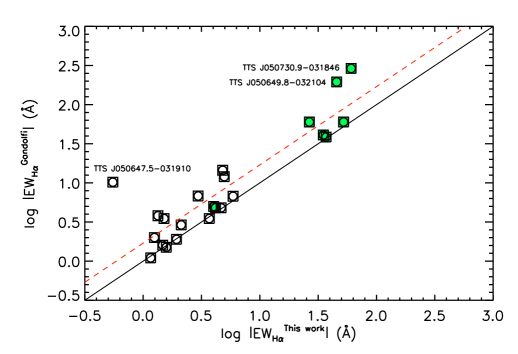
Figure 1: Comparison between our $EW_{\rm H\alpha}$ values and those obtained by Gandolfi et al. (2008). The solid line represents the 1:1 relation, while the dashed one is shifted by the r.m.s. difference between the $\log EW_{\rm H\alpha}$ values (excluding the three most deviating objects labeled in the figure). Filled symbols refer to most-probable accreting stars (see text and Fig. 2).

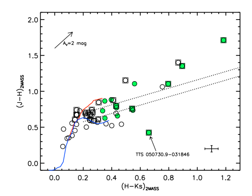
Figure 2: 2MASS color-color diagram of the L1615/L1616 targets. Open circles represent low-mass stars analyzed by Gandolfi et al. (2008), while squares mark the targets observed for this work with the FLAMES spectrograph. Filled symbols are the most probable accretors as defined in Section 2.2. The dwarf (lower branch; Bessell & Brett 1988) and the giant (upper branch; Kenyon & Hartmann 1995) sequences are marked by solid lines. The arrow at the top upper-left corner indicates the reddening vector for $A_{V}=2$ mag. The CTTs locus (Meyer et al. 1997) is delimited by the dotted lines. The position of the sub-luminous candidate TTS 050730.9$-$031846 is also displayed. The mean 2MASS photometric errors are overplotted on the lower-right corner of the panel.

3 Accretion diagnostics and mass accretion rates

According to the magnetospheric accretion model (Uchida & Shibata 1985; Königl 1991; Shu et al. 1994), matter is accreted from the disk onto the star and shocks the stellar surface producing high temperature ($\sim 10^{4}$ K) gas, giving rise to emission in the blue continuum and in many lines, which can be observed as photometric and spectroscopic diagnostics. Primary accretion diagnostics, such as the UV excess emission, the Paschen/Balmer continua, and the Balmer jump (see, e.g., Herczeg & Hillenbrand 2008; Alcalá et al. 2014), and secondary tracers, like hydrogen recombination lines and the He i, Ca ii, Na i lines (see, e.g., Muzerolle et al. 1998; Antoniucci et al. 2011; Biazzo et al. 2012) are therefore useful tools to detect accretion signatures and to derive the energy losses due to accretion, i.e. the accretion luminosity (e.g., Gullbring et al. 1998; Herczeg & Hillenbrand 2008; Rigliaco et al. 2011b; Ingleby et al. 2013; Alcalá et al. 2014).

In the context of the magnetospheric accreting model, the accretion luminosity can be converted into mass accretion rate, $\dot{M}_{\rm acc}$, using the following relationship (Hartmann 1998):

$$\dot{M}_{\rm acc}=\left(1-\frac{R_{\star}}{R_{\rm in}}\right)^{-1}\frac{L_{\rm acc}R_{\star}}{GM_{\star}}\,\approx 1.25\frac{L_{\rm acc}R_{\star}}{GM_{\star}}\,,$$ (1)

where $M_{\star}$ and $R_{\star}$ are the stellar mass and radius, respectively, $R_{\rm in}$ is the YSO inner-disk radius, and $G$ is the universal gravitational constant. $R_{\rm in}$ corresponds to the distance at which the disk is truncated – due to the stellar magnetosphere – and from which the disk gas is accreted, channeled by the magnetic field lines. In previous works, it has been assumed that $R_{\rm in}$ is $\sim 5\,R_{\star}$ (see, e.g., Alcalá et al. 2011).

The accretion luminosity can be estimated from empirical linear relationships between the observed line luminosity, $L^{\lambda}$, and $L_{\rm acc}$ derived through primary diagnostics (see, e.g., Gullbring et al. 1998; Herczeg & Hillenbrand 2008; Alcalá et al. 2014). Such relationships have been established by the simultaneous observations of many accretion indicators and by modeling the continuum excess emission.

For the accretors in our sample, we used the luminosity of several emission lines (H$\alpha$ $\lambda$6563 Å, H$\beta$ $\lambda$4861 Å, He i $\lambda$5876 Å, He i $\lambda$6678 Å, and He i $\lambda$7065 Å) within the wavelength range covered by the FLAMES spectra, while for the objects in Gandolfi et al. (2008) we used the H$\alpha$ line. We then considered the recent $L^{\lambda}-L_{\rm acc}$ relations by Alcalá et al. (2014) to derive the accretion luminosity from each line. These relationships consider a combination of all accretion indicators calibrated on sources for which the UV excess emission and the Paschen/Balmer continua were measured simultaneously.

Unfortunately, we do not have simultaneous or quasi-simultaneous photometry in hand and our fiber-fed spectra cannot be calibrated in flux. Therefore, the best approach to calculate line luminosities from our data is by deriving line surface fluxes using the equivalent widths and assuming continuum fluxes from model atmospheres. Thus, the line luminosity $L^{\lambda}$ was calculated using the same approach as in Biazzo et al. (2012). In particular, $L^{\lambda}=4\pi R_{\star}^{2}F^{\lambda}$, where the stellar radius was taken from Gandolfi et al. (2008) and the surface flux, $F^{\lambda}$, was derived by multiplying the EW of each line ($EW_{\lambda}$) by the continuum flux at wavelengths adjacent to the line ($F_{\rm cont}^{\lambda\pm\Delta\lambda}$). The latter was gathered from the NextGen Model Atmospheres (Hauschildt et al. 1999), assuming the corresponding YSO effective temperature and surface gravity. The gravity was estimated for every YSO from the mass and stellar radius reported in Gandolfi et al. (2008). In particular, we considered the three different $M_{\star}$ values provided by the authors for three different sets of PMS evolutionary tracks (namely, Baraffe et al. 1998 and Chabrier et al. 2000, D’Antona & Mazzitelli 1997, Palla & Stahler 1999; hereafter Ba98+Ch00, DM97, PS99, respectively, as used in Gandolfi et al. 2008). We stress that the mean difference in $\log g$ coming from the use of the three evolutionary tracks varies from $\sim$0.0 to 0.4 dex. Such a kind of differences in $\log g$ may lead to an uncertainty in the continuum flux of less than $\sim 10\%$, mainly depending on the effective temperature, the surface gravity itself, and the line considered. This represents the typical error in the continuum flux we considered for the estimation of the uncertainty in $\dot{M}_{\rm acc}$ (see text later on).

In the end, the different line diagnostics considered by us yielded consistent values of $L_{\rm acc}$, which justified the use of all of them to compute an average $\langle L_{\rm acc}\rangle$ for each YSO (see Table 3). In this way, the error on the average $L_{\rm acc}$ derived from several diagnostics, measured simultaneously, is minimized, as found by Rigliaco et al. (2012) and Alcalá et al. (2014). The mass accretion rate ($\dot{M}_{\rm acc}$) was then calculated using $\langle L_{\rm acc}\rangle$ and the Eq. 1, and adopting the $M_{\star}$ and $R_{\star}$ values reported in Gandolfi et al. (2008). For every accretor, we thus derived three values of $\dot{M}_{\rm acc}$ using the three values of $M_{\star}$ (Table 3).

Contributions to the error budget on $\dot{M}_{\rm acc}$ include uncertainties on stellar mass, stellar radius, inner-disk radius, and $L_{\rm acc}$. Assuming mean errors of $\sim 0.1M_{\odot}$ in $M_{\star}$ and $\sim 0.1R_{\odot}$ in $R_{\star}$ (Gandolfi et al. 2008), $1-13\%$ as relative error in $EW_{\lambda}$, 10% in $F_{\rm cont}^{\lambda\pm\Delta\lambda}$, and the uncertainties in the relationships by Alcalá et al. (2014), we estimate a typical error in $\log\dot{M}_{\rm acc}$ of $\sim 0.5$ dex.

Note that the equivalent width values are not corrected for veiling, which alters the continuum of the spectra. In case of strong accretors, the continuum excess emission becomes important, but we quantify this effect on our sample in the next section.

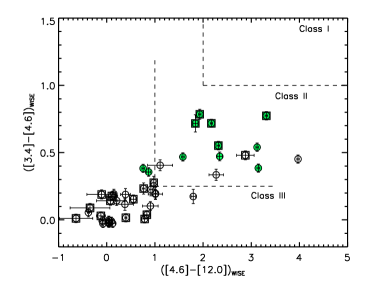
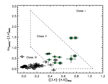
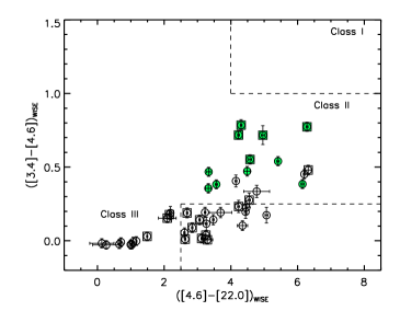
Figure 3: WISE/2MASS color-color diagrams of the L1615/L1616 targets. Dashed lines indicate the boundaries of Class I, Class II, and disk-less stars (Class III objects) as defined in Koenig et al. (2012). The non-accretors falling within the Class II region will be discussed in Appendix C. Symbols are as in Fig. 2.

3.1 Impact of veiling on the $\dot{M}_{\rm acc}$ estimates

We estimate how the amount of veiling affects the $\dot{M}_{\rm acc}$ estimates by running the ROTFIT code (Frasca et al. 2003, 2006) on the spectra of our accretors. This code compares the target spectrum with a grid of slowly-rotating and low-activity templates, aligned with the target spectrum, re-sampled on its spectral points, and artificially broadened with a rotational profile until the minimum of the residuals is reached (see details in Frasca et al. 2014, submitted). In order to find the best template reproducing the veiled accretors, we included the veiling as an additional parameter. This was done by adding a featureless veiling to each template, whose continuum-normalized spectrum becomes:

$$\Biggl{(}\frac{F_{\lambda}}{F_{\rm cont}}\Biggr{)}^{veil}=\frac{\Bigl{(}\frac{F_{\lambda}}{F_{\rm cont}}\Bigr{)}+veil}{1+veil}\,.$$ (2)

This procedure could be applied only to 5 accretors in our sample. Unfortunately, the low resolution of the spectra acquired by Gandolfi et al. (2008) and the very low $S/N$ ratio of some FLAMES spectra were not sufficient to apply our method.

In Fig. 4 we show an example of an accreting star observed with UVES (LkH$\alpha$ 333), with $veil=0.5$, as found by ROTFIT. In Table 2, we list the mean veiling derived from the FLAMES spectra. Using these values, we could estimate the new $\dot{M}_{\rm acc}$ correcting the measured EWs of the lines by the factor $(1+veil)$. We can conclude that the correction for the veiling leads to a difference of $\sim$ 0.25 dex in $\log\dot{M}_{\rm acc}$ at most, i.e. within the errors of our estimates and not affecting our conclusions. Similar results were also found by Costigan et al. (2012). Hereafter, as we could not evaluate the veiling for all our targets, we will adopt the $\dot{M}_{\rm acc}$ without any correction for the veiling.

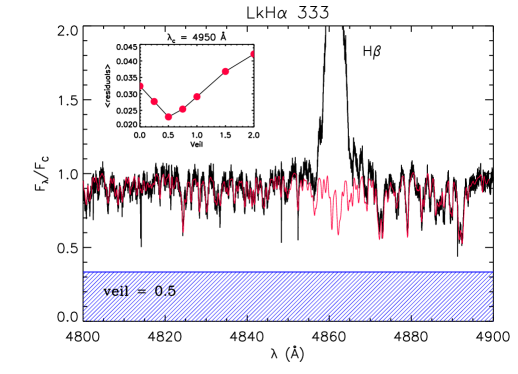
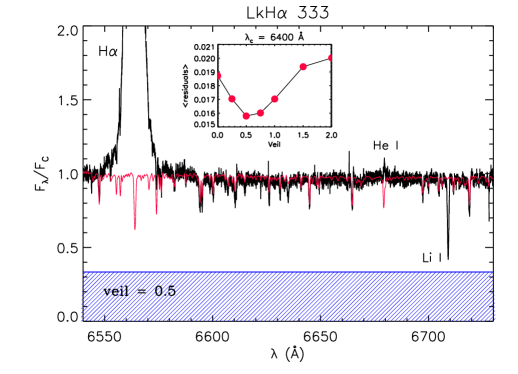
Figure 4: Example of UVES spectrum of the accreting star LkH$\alpha$ 333 both in the H$\beta$ (left panel) and in the H$\alpha$ (right panel) region. In both panels, the black solid line represents the spectrum of the target, while the red solid line is the spectrum of the best template reproducing the target at $veil=0.5$. The residuals as a function of the $veil$ parameter are plotted in the inset. The hatched area is the level of the veiling at 0.5.

Table 2: Mean veiling and difference in $\log\dot{M}_{\rm acc}$ for the targets for which we could run the ROTFIT code.

ID Name	$veil$	$\Delta\log\dot{M}_{\rm acc}$
		(dex)
TTS J050646.1$-$031922	0.50	0.25
RX J0506.9$-$0319 SE	0.25	0.10
LkH$\alpha$ 333	0.50	0.20
L1616 MIR 4	0.50	0.20
RX J0507.1$-$0321	0.50	0.20

3.2 Variability

Being based on single “epoch” measurements of line equivalent widths and continuum fluxes estimates, our calculations of line luminosity and accretion luminosity represent only an instantaneous snapshot of $L_{\rm acc}$ and $\dot{M}_{\rm acc}$. As in previous investigations in other star forming regions (SFRs; see, e.g., Nguyen et al. 2009; Biazzo et al. 2012; Costigan et al. 2012; Fang et al. 2013; Costigan et al. 2014), and based on multi-epoch observations of several of our targets, we estimate that short-time scale ($\sim$48 hours) variations may induce a scatter on $\log\dot{M}_{\rm acc}$ of $<0.3$ dex, while at a longer time scale (a few years) it may be up to $\sim 0.6$ dex (see Appendix C.3). Therefore, as claimed in those studies, here we also conclude that YSOs variability may account for variations in $\log\dot{M}_{\rm acc}$ in the range of $\sim 0.2-0.6$ dex.

4 Results and discussion

In the following, we discuss the accretion properties of the sample and their link with the stellar parameters and the IR colors.

4.1 Accretion luminosity versus stellar parameters

At low levels of accretion, the chromospheric emission may have an important impact on the estimates of $L_{\rm acc}$ (see Manara et al. 2013, and references therein). This contribution should be therefore considered when accretion properties are studied. As shown in Fig. 5, the accretion luminosity of the YSOs in L1615/L1516 decreases monotonically with the effective temperature. The dashed line in this figure shows the chromospheric level as determined by Manara et al. (2013), and represents the locus below which the contribution of chromospheric emission starts to be important in comparison with energy losses due to accretion. All accreting YSOs in L1615/L1616 fall well above the “systematic noise” due to chromospheric emission and show $L_{\rm acc}/L_{\odot}$ very similar to the values recently derived for members of the Lupus SFR by Alcalá et al. (2014) and estimated through primary diagnostics.

Figure 6 shows the mean accretion luminosity as a function of the stellar luminosity. As already observed by previous investigations in other SFRs, like $\rho$ Ophiucus, Taurus, and Lupus (Muzerolle et al. 1998; Natta et al. 2006; Alcalá et al. 2014), the accretion luminosity increases with the stellar luminosity. In our sample of accreting stars, $L_{\rm acc}$ follows a trend which is similar to the recent power-law found by Alcalá et al. (2014) in the Lupus star-forming region. Moreover, the dispersion of our data points in $L_{\rm acc}$ is similar. As in other star forming regions, the accretion luminosity of the YSOs in L1615/L1616 is a fraction of the stellar luminosity, and falls in the range between 0.1$L_{\star}$ to 0.01$L_{\star}$ (see, e.g., Muzerolle et al. 1998; White & Hillenbrand 2004; Antoniucci et al. 2011; Caratti o Garatti et al. 2012; Alcalá et al. 2014).

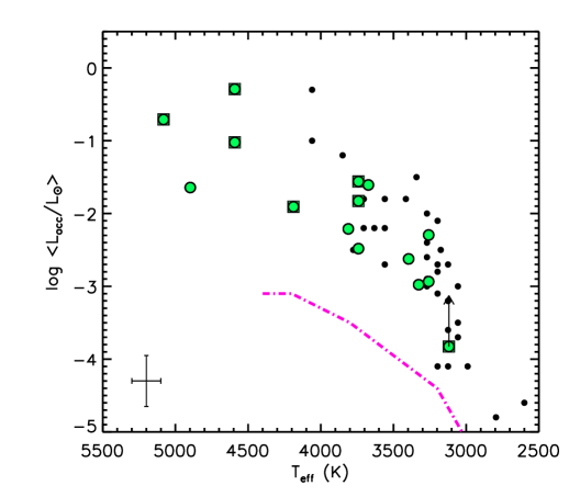
Figure 5: Mean accretion luminosity versus effective temperature. The dash-dotted line marks the locus below which chromospheric emission is important in comparison with $L_{\rm acc}$ (Manara et al. 2013). The vertical arrow represents the position of the sub-luminous object after applying the correction factor described in Appendix C.1. Small filled dots represent the Alcalá et al. (2014) sample of low-mass stars in the Lupus SFR. Mean error bars are overplotted on the lower-left corner of the panel. Symbols are as in Fig. 2.

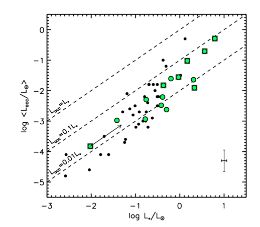
Figure 6: Mean accretion luminosity versus stellar luminosity. The dashed lines represent the loci of the three $L_{\rm acc}-L_{\star}$ relations, as labeled. The arrow represents the position of the sub-luminous object after applying the correction factor described in Appendix C.1. The Lupus YSOs by Alcalá et al. (2014) are overlaid as small filled dots. Mean error bars are overplotted on the lower-right corner of the panel. Symbols are as in Fig. 2.

4.2 Mass accretion rate versus stellar mass

The distribution of YSOs in the $\dot{M}_{\rm acc}$ versus $M_{\star}$ plane provides an important diagnostic for the studies of the evolution of mass accretion (see Hartmann et al. 2006). The $\dot{M}_{\rm acc}$ versus $M_{\star}$ relationship has been obtained for a number of different star-forming regions (e.g., Taurus, Ophiuchus, $\sigma$ Orionis, Orion Nebula Cluster, Trumpler 37). In all regions studied so far it has been found that, although there is a rough correlation of $\dot{M}_{\rm acc}$ with the square of $M_{\star}$, the scatter of $\dot{M}_{\rm acc}$ for a given mass is very large (e.g., Muzerolle et al. 2005; Natta et al. 2006).

The physical origin of the $\dot{M}_{\rm acc}\propto M_{\star}^{\alpha}$ relationship, with $\alpha\approx 2$, is still unclear. Alexander & Armitage (2006) have suggested that the correlation reflects the initial conditions established when the disk formed, followed by subsequent viscous disk evolution of the disk. The natural decline of the mass accretion rate with age in viscous disk evolution and effects due to evolutionary differences within a sample have been ruled out as possible cause for the large spread of the relationship within individual star forming regions (Mohanty et al. 2005; Natta et al. 2006). Moreover, short-term (see, e.g., Nguyen et al. 2009; Biazzo et al. 2012) and long-term variability may contribute to, but cannot explain the large vertical spread of the $\dot{M}_{\rm acc}-M_{\star}$ relationship (Biazzo et al. 2012; Costigan et al. 2012, 2014). It appears more likely related to a spread in the properties of the parental cores, their angular momentum in particular (e.g., Hartmann et al. 2006; Dullemond et al. 2006), in stellar properties, such as X-ray emission (Muzerolle et al. 2003), or on the competition between different accretion mechanisms, such as viscosity and gravitational instabilities (Vorobyov & Basu 2008). As opposed to Dullemond et al. (2006), Ercolano et al. (2014) argued that the $\dot{M}_{\rm acc}$ versus $M_{\star}$ relation for a population of disks dispersing via X-ray photo-evaporation is completely determined by the shape of the X-ray luminosity function, hence requires no spread in initial conditions other than the dependence on stellar mass. On the other hand, Alcalá et al. (2014) have concluded that mixing mass-accretion rates calculated with different techniques may increase the scatter in the $\dot{M}_{\rm acc}$ versus $M_{\star}$ relationship. They also have claimed that the different methodologies used to derive accretion luminosity and line luminosity, as well as the different evolutionary models used to estimate masses may lead to significantly different results on the slope of the relationship.

The results in the $\dot{M}_{\rm acc}-M_{\star}$ plane for our sample of accretors in L1615/L1616 are shown in Fig. 7. The three panels in this figure correspond to the values of $\dot{M}_{\rm acc}$ calculated from the three estimates of $M_{\star}$ drawn from the three evolutionary models, as labeled in the figure. Since our number statistics is low, we do not attempt a linear fit to the $\dot{M}_{\rm acc}-M_{\star}$ relationships, but for comparison, we overplot the $\dot{M}_{\rm acc}-M_{\star}$ linear fit with a slope of $1.8\pm 0.2$ recently calculated for Lupus YSOs (Alcalá et al. 2014), for which the accretion luminosity was directly derived by modeling the excess emission from the UV to the near-infrared as the continuum emission of a slab of hydrogen. Similar findings were also obtained in other T associations, like Taurus or Chamaeleon (see, e.g., Herczeg & Hillenbrand 2008; Antoniucci et al. 2011; Biazzo et al. 2012).

The accretors in L1615/L1616 follow closely the $\dot{M}_{\rm acc}-M_{\star}$ relationship seen for the YSOs in Lupus by Alcalá et al. (2014), but interestingly the scatter changes depending on the evolutionary tracks used to derive the stellar masses. As concluded in Appendix B, the different evolutionary tracks have negligible effects on the computation of $\log\dot{M}_{\rm acc}$, meaning that the scatter in the $\log\dot{M}_{\rm acc}-\log M_{\star}$ diagram is mainly induced by the uncertainty on the mass, which is model-dependent. The DM97 tracks seem to produce the largest scatter.

We stress, however, that some scatter in the $\dot{M}_{\rm acc}-M_{\star}$ relationship (up to around $\pm 0.5-0.6$ dex in $\log\dot{M}_{\rm acc}$; see, e.g., Costigan et al. 2014, and references therein) may come from intrinsic variability, as our line luminosity determinations were obtained from single “epoch” measurements of line equivalent widths and assuming continuum flux coming from model atmospheres (see Section 3.2).

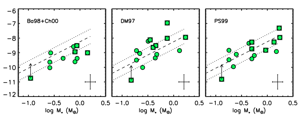
Figure 7: Mass accretion rate versus stellar mass drawn from the Ba98+Ch00, DM97, and PS99 evolutionary tracks, respectively from the left to the right panel. The dashed and dotted lines represent the $\dot{M}_{\rm acc}-M_{\star}$ relationship and the $1\sigma$ deviation from the fit obtained with X-Shooter@VLT observations by Alcalá et al. (2014) for YSOs in Lupus. The vertical arrow represents the position of the sub-luminous object after applying the correction factor described in Appendix C.1. Mean error bars are overplotted on the lower-right corner of each panel. Symbols are as in Fig. 2.

4.3 Accretion versus infrared properties

Near- and mid-IR colors can be used to probe the inner disk region. Hartigan et al. (1995), studying a sample of 42 T-Tauri stars and using the $K-L$ color excesses, pointed out that disk dissipation is mainly due to the formation of micron-sized dust particles, which merge together to create planetesimals and protoplanets at the end of the CTTs phase. Protoplanets may clear the innermost part of the disk where the gas and dust have temperature of the order of $\sim$ 1000 K and emit mainly at near-IR and mid-IR wavelengths. This causes the disk to decrease or loose its near-IR color excess and at the same time the opening of a gap in the disk (see, e.g., Lin & Papaloizou 1993), thereby possibly terminating accretion from the disk onto the star.

With the aim of investigating possible relationships between IR colors and accretion properties, we plotted in Fig. 8 the $J-H$, $H-K{\rm s}$, $J-K{\rm s}$ $2MASS$ colors and the [3.4]$-$[4.6], [4.6]$-$[12.0], [4.6]$-$[22.0] $WISE$ colors as a function of the mass accretion rates derived using the PS99 tracks, from which masses could be estimated for all the accretors we studied in this work. Despite the poor statistics, the behavior of the $2MASS$ and $WISE$ colors with accretion is different. While the $2MASS$ colors tend to rise at $\dot{M}_{\rm acc}\raisebox{-2.15277pt}{$\>\stackrel{{\scriptstyle\textstyle>}}{{\sim}}\>$}10^{-10}M_{\odot}$ yr^-1, the $WISE$ ones show no trend with $\dot{M}_{\rm acc}$. In order to quantify the degree of possible correlations in Fig. 8, we computed the Spearman’s rank correlation coefficients with the IDL platform. These correlation coefficients, ranging from 0 to 1, show values around 0.6 for the relations between $\dot{M}_{\rm acc}$ and $2MASS$ colors, and values very close to zero for the $WISE$ colors, meaning that the $2MASS$ colors show an increasing trend with $\log\dot{M}_{\rm acc}$, while no trend is detected for the relations between $\dot{M}_{\rm acc}$ and the $WISE$ colors.

The trend between $2MASS$ colors and $\log\dot{M}_{\rm acc}$ could be an indication that objects with strong accretion have optically thick inner disks, as found in previous works (Hartigan et al. 1995; Rigliaco et al. 2011a; Biazzo et al. 2012). In particular, we can identify the regions $\log\dot{M}_{\rm acc}\raisebox{-2.15277pt}{$\>\stackrel{{\scriptstyle\textstyle>}}{{\sim}}\>$}-8.5$ dex and $J-H\raisebox{-2.15277pt}{$\>\stackrel{{\scriptstyle\textstyle>}}{{\sim}}\>$}$ 1.0 or $H-K{\rm s}\raisebox{-2.15277pt}{$\>\stackrel{{\scriptstyle\textstyle>}}{{\sim}}\>$}$ 0.7 or $J-K{\rm s}\raisebox{-2.15277pt}{$\>\stackrel{{\scriptstyle\textstyle>}}{{\sim}}\>$}$ 1.75 as those where strong accreting objects with large near-IR excess are found in L1615/L1616.

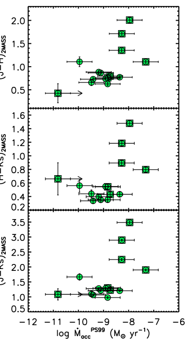
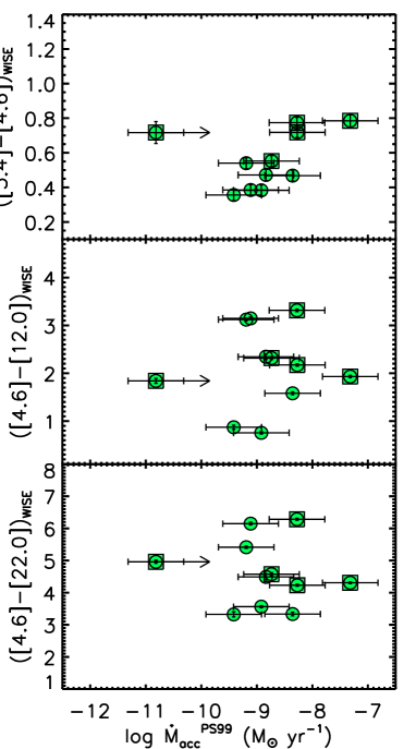
Figure 8: 2MASS (left panel) and WISE (right panel) colors versus mass accretion rates derived using the PS99 stellar masses. The horizontal arrows represent the position of the sub-luminous object after correction of $\dot{M}_{\rm acc}$, as explained in Appendix C.1. Symbols are as in Fig. 2.

5 Conclusions

In this paper, we investigated the accretion and the IR properties of YSOs in the cometary cloud L1615/L1616 in Orion. For this purpose we used intermediate resolution (FLAMES@VLT) and low-resolution (FORS2@VLT + VIMOS@VLT) optical spectroscopy for 23 and 31 objects, respectively. Our main results can be summarized as follows:

1. The YSOs in L1615/L1616 observed with FLAMES show a narrow distribution in radial velocity peaked at $23.2\pm 3.1$ km s^-1, showing they are dynamically associated with the cloud, and mean lithium abundance of $3.3\pm 0.3$ dex confirming their membership to the cometary cloud and their youth.

2. The fraction of accretors in L1615/L1516 is close to 30%, consistent with the fraction of disks recently reported by Ribas et al. (2014) for an average age of 3 Myr.

3. The mass accretion rates ($\dot{M}_{\rm acc}$) derived through several secondary diagnostics (H$\alpha$, H$\beta$, He i $\lambda$5876 Å, He i $\lambda$6678 Å, and He i $\lambda$7065 Å) are in the range $\sim 10^{-10}-10^{-7}M_{\odot}$ yr^-1 for stars with $\sim 0.1-2.3M_{\odot}$. These accretion rates are similar to those of YSOs of similar mass in other star forming regions.

4. The accretion properties of the YSOs in L1615/L1616 have the same behavior as YSOs in other star-forming regions, like Lupus or Taurus. This might imply that environmental conditions at which the cometary cloud is exposed uninfluenced the accretion evolution of the YSOs in this cometary cloud.

5. As recently found by other authors, we confirm that different methods used to derive stellar parameters and mass accretion rates introduce dispersion in the $\dot{M}_{\rm acc}-M_{\star}$ relation; in particular, the differences in the evolutionary tracks used to derive $M_{\star}$ and then $\dot{M}_{\rm acc}$ produce a scatter in the $\dot{M}_{\rm acc}-M_{\star}$ relationship, but no significant systematic effect on $\dot{M}_{\rm acc}$.

6. The color$-\dot{M}_{\rm acc}$ diagrams suggest that strong accretors (i.e. those with $\log\dot{M}_{\rm acc}\raisebox{-2.15277pt}{$\>\stackrel{{\scriptstyle\textstyle>}}{{\sim}}\>$}-8.5$ dex) show large excesses in the $JHK{\rm s}$ bands, indicative of inner optically thick disk, as in previous studies.

[x]lccccccc Observing log, radial velocity, and lithium content for the stars observed with FLAMES.
ID name $JD$ Instrument # $V_{\rm rad}$ $EW_{\rm Li}$ $\log n({\rm Li})$ Comment
($+2\,450\,000$) obs. (km s^-1) (mÅ) (dex)
TTS J050646.1$-$0319223797.0722 GIRAFFE 2 26.2$\pm$6.6 587 3.70 N1,N2;S1,S2
3797.1097 ” 25.9$\pm$6.9 594 N1,N2;S1,S2
RX J0506.8$-$0318 3795.0535 GIRAFFE 3 21.6$\pm$0.7 604 3.15
3795.1009 ” 21.7$\pm$2.7 605
3796.0344 ” 22.6$\pm$0.3 581
TTS J050647.5$-$0319103795.0535 GIRAFFE 3 … … … LSN
3795.1009 ” 28.6$\pm$5.3 …
3796.0344 ” … … LSN
RX J0506.8$-$0327 3795.0535 GIRAFFE 2 26.3$\pm$2.3 566 3.50
3795.1009 ” 26.8$\pm$1.8 550
RX J0506.8$-$0305 3796.0344 GIRAFFE 1 19.1$\pm$4.0 565 3.35
TTS J050649.8$-$0321043795.1009 GIRAFFE 2 … … LSN
3796.0344 ” … … LSN
RX J0506.9$-$0319 NW 3795.1009 GIRAFFE 1 21.3$\pm$2.2 412 2.70
RX J0506.9$-$0319 SE 3797.0722 GIRAFFE 2 27.4$\pm$5.8 565 3.40 N1,N2;S1,S2
3797.1097 ” 27.2$\pm$4.7 601 N1,N2;S1,S2
RX J0506.9$-$0320 W 3795.0535 GIRAFFE 1 21.4$\pm$1.6 562 3.35
RX J0506.9$-$0320 E 3796.0344 GIRAFFE 4 22.9$\pm$3.3 409 3.70
3797.0298 ” 23.5$\pm$3.3 444
3797.0722 ” 24.3$\pm$4.4 385
3797.1096 ” 23.9$\pm$5.6 377
LkH$\alpha$ 333 3796.0344 GIRAFFE 1 25.9$\pm$1.6 447 3.50
3795.0535 UVES 6 27.0$\pm$0.5 508 O1,O2; T
3795.1009 ” … … LSN
3796.0767 ” 27.8$\pm$0.5 462 O1,O2
3797.0298 ” 28.4$\pm$0.6 455 O1,O2
3797.1097 ” 28.2$\pm$2.0 437 O1,O2
3797.0723 ” 27.9$\pm$1.1 455 O1,O2
L1616 MIR 4 3795.1009 GIRAFFE 4 24.3^a 365 3.50
3797.0298 ” 29.4$\pm$7.9 … LSN
3797.0722 ” 28.1^a … LSN
3797.1097 ” … … LSN
RX J0507.0$-$0318 3795.0535 GIRAFFE 3 23.1$\pm$2.7 556$>$3.50
3795.1009 ” 23.7$\pm$1.9 583 T
3796.0344 ” 23.6$\pm$1.7 601
RX J0507.1$-$0321 3795.0535 GIRAFFE 2 20.9$\pm$1.1 575$>$3.50
3796.0344 ” 21.9$\pm$1.8 550
RX J0507.2$-$0323 3796.0767 GIRAFFE 1 24.8$\pm$1.7 525 3.40 T
RX J0507.3$-$0326 3795.0535 GIRAFFE 2 21.4$\pm$1.1 549 3.40
3796.0767 ” 21.8$\pm$1.8 545
TTS J050717.9$-$0324333795.0535 GIRAFFE 2 20.2^a 524 3.50
3796.0767 ” 20.4^a 530
RX J0507.4$-$0320 3795.0535 GIRAFFE 3 20.3^a 587 3.50
3796.0767 ” 19.8^a 518
3796.0344 ” 19.9^a 608
RX J0507.4$-$0317 3795.0535 GIRAFFE 3 19.8$\pm$6.4 … 3.20 LSN
3796.0767 ” 19.2^a 457
3796.0344 ” 20.0^a 503
TTS J050729.8$-$0317053795.0535 GIRAFFE 3 … … 3.00 LSN
3796.0767 ” … … LSN
3796.0344 ” … 580
TTS J050730.9$-$0318463795.0535 GIRAFFE 2 … … … LSN
3796.0344 ” … … LSN
TTS J050734.8$-$0315213795.0535 GIRAFFE 3 … … … LSN
3796.0767 ” … … LSN
3796.0344 ” … … LSN
RX J0507.6$-$0318 3795.0535 GIRAFFE 3 20.3$\pm$2.7 567 2.75
3796.0767 ” 19.2$\pm$1.7 524
3796.0344 ” 19.5$\pm$4.1 544
Notes: ^a Due to low $S/N$ ratio, few lines, late spectral type, and/or short wavelength coverage, the radial velocity error may be up to 60%. LSN: low $S/N$ spectrum; T: template spectrum used for the CCF analysis. Some optical forbidden lines are observed in emission: O1=[O i] $\lambda$6300.8 Å, O2=[O i] $\lambda$6363.8 Å, S1=[S ii] $\lambda$6715.8 Å, S2=[S ii] $\lambda$6729.8 Å, N1=[N ii] $\lambda$6548.4 Å, N2=[N ii] $\lambda$6583.4 Å.

[x]lccc—cccc Near-IR and Mid-IR photometric data.
2MASS WISE
ID name $J$ $H$ $K$s [3.4] [4.6] [12.0] [22.0]
(mag) (mag) (mag) (mag) (mag) (mag) (mag)
1RXS J045912.4$-$033711 10.070$\pm$0.022 9.616$\pm$0.024 9.474$\pm$0.020 9.386$\pm$0.023 9.395$\pm$0.018 9.299$\pm$0.033 8.691^b
1RXS J050416.9$-$021426 10.661$\pm$0.024 10.105$\pm$0.024 9.984$\pm$0.025 9.910$\pm$0.023 9.936$\pm$0.020 9.812$\pm$0.048 8.943^b
TTS J050513.5$-$034248 15.120$\pm$0.041 14.598$\pm$0.053 14.198$\pm$0.065 14.011$\pm$0.030 13.837$\pm$0.044 12.041^b 8.769^b
TTS J050538.9$-$032626 13.287$\pm$0.024 12.601$\pm$0.022 12.387$\pm$0.024 12.196$\pm$0.024 12.093$\pm$0.023 11.186$\pm$0.159 7.745$\pm$0.152
RX J0506.6$-$0337 10.657$\pm$0.022 10.304$\pm$0.027 10.205$\pm$0.023 10.130$\pm$0.024 10.138$\pm$0.021 10.226$\pm$0.070 9.067^b
TTS J050644.4$-$032913 13.641$\pm$0.028 13.038$\pm$0.031 12.779$\pm$0.032 12.613$\pm$0.025 12.421$\pm$0.025 11.411$\pm$0.146 8.731$\pm$0.336
TTS J050646.1$-$031922 13.218$\pm$0.025 11.506$\pm$0.025 10.322$\pm$0.023 8.866$\pm$0.023 8.148$\pm$0.018 5.976$\pm$0.014 3.918$\pm$0.026
RX J0506.8$-$0318 11.849$\pm$0.023 11.108$\pm$0.025 10.955$\pm$0.023 10.835$\pm$0.023 10.819$\pm$0.020 10.422^b 7.696^b
TTS J050647.5$-$031910 14.286$\pm$0.030 13.410$\pm$0.030 12.999$\pm$0.023 12.586$\pm$0.024 12.106$\pm$0.023 9.229$\pm$0.180 5.786$\pm$0.091
RX J0506.8$-$0327 11.599$\pm$0.023 10.855$\pm$0.027 10.595$\pm$0.026 10.584$\pm$0.024 10.430$\pm$0.020 9.877$\pm$0.047 8.337$\pm$0.263
RX J0506.8$-$0305 12.939$\pm$0.021 12.281$\pm$0.025 12.058$\pm$0.028 11.951$\pm$0.025 11.762$\pm$0.023 11.868$\pm$0.305 9.073^b
TTS J050649.8$-$031933 12.391$\pm$0.022 11.526$\pm$0.027 11.175$\pm$0.026 10.747$\pm$0.023 10.362$\pm$0.020 7.215$\pm$0.020 4.214$\pm$0.037
TTS J050649.8$-$032104 12.699$\pm$0.026 11.346$\pm$0.026 10.452$\pm$0.028 9.845$\pm$0.023 9.071$\pm$0.021 5.756$\pm$0.016 2.787$\pm$0.022
TTS J050650.5$-$032014 13.663$\pm$0.026 12.971$\pm$0.027 12.541$\pm$0.030 … … … …
TTS J050650.7$-$032008 13.642$\pm$0.057 12.984$\pm$0.037 12.544$\pm$0.043 … … … …
RX J0506.9$-$0319 NW 11.324^a 11.939$\pm$0.072 10.007^a … … … …
RX J0506.9$-$0319 SE 10.809^a 10.050$\pm$0.041 9.507^a … … … …
RX J0506.9$-$0320 W 10.042$\pm$0.040 8.889$\pm$0.042 8.393$\pm$0.039 … … … …
RX J0506.9$-$0320 E 10.366$\pm$0.023 8.965$\pm$0.027 8.099$\pm$0.026 … … … …
TTS J050654.5$-$032046 15.984$\pm$0.082 14.878$\pm$0.066 14.318$\pm$0.070 … … … …
LkH$\alpha$ 333 10.343$\pm$0.022 9.239$\pm$0.024 8.443$\pm$0.025 6.981$\pm$0.030 6.196$\pm$0.021 4.265$\pm$0.013 1.888$\pm$0.018
L1616 MIR 4 13.010$\pm$0.045 11.003$\pm$0.035 9.524$\pm$0.025 … … … …
RX J0507.0$-$0318 11.190$\pm$0.022 10.344$\pm$0.027 10.036$\pm$0.023 9.975$\pm$0.024 9.937$\pm$0.020 9.103$\pm$0.051 6.687$\pm$0.099
TTS J050657.0$-$031640 13.040$\pm$0.023 12.414$\pm$0.025 12.062$\pm$0.023 11.781$\pm$0.024 11.309$\pm$0.022 8.964$\pm$0.052 6.820$\pm$0.092
TTS J050704.7$-$030241 14.809$\pm$0.036 14.208$\pm$0.049 13.964$\pm$0.059 13.795$\pm$0.029 13.569$\pm$0.037 12.652^b 9.104^b
TTS J050705.3$-$030006 12.517$\pm$0.023 11.789$\pm$0.027 11.614$\pm$0.025 11.594$\pm$0.023 11.539$\pm$0.023 11.919^b 8.931^b
RX J0507.1$-$0321 12.153$\pm$0.025 11.357$\pm$0.027 10.926$\pm$0.022 10.656$\pm$0.023 10.104$\pm$0.022 7.787$\pm$0.021 5.530$\pm$0.043
TTS J050706.2$-$031703 14.660$\pm$0.033 14.067$\pm$0.041 13.820$\pm$0.048 13.498$\pm$0.027 13.163$\pm$0.032 10.891$\pm$0.145 8.390$\pm$0.387
RX J0507.2$-$0323 11.659$\pm$0.020 11.053$\pm$0.025 10.911$\pm$0.025 10.806$\pm$0.022 10.799$\pm$0.021 10.012$\pm$0.060 7.505$\pm$0.160
TTS J050713.5$-$031722 13.918$\pm$0.031 12.855$\pm$0.030 12.100$\pm$0.030 … … … …
RX J0507.3$-$0326 11.454$\pm$0.021 10.780$\pm$0.024 10.628$\pm$0.022 10.508$\pm$0.023 10.478$\pm$0.019 10.599$\pm$0.090 8.989^b
TTS J050717.9$-$032433 13.099$\pm$0.021 12.426$\pm$0.028 12.178$\pm$0.028 12.112$\pm$0.024 12.023$\pm$0.023 12.369$\pm$0.412 9.182^b
RX J0507.4$-$0320 12.305$\pm$0.024 11.716$\pm$0.025 11.440$\pm$0.023 11.305$\pm$0.023 11.127$\pm$0.022 11.021$\pm$0.114 8.968^b
RX J0507.4$-$0317 13.173$\pm$0.026 12.469$\pm$0.027 12.254$\pm$0.029 12.161$\pm$0.023 12.019$\pm$0.024 11.943$\pm$0.285 8.956^b
TTS J050729.8$-$031705 14.937$\pm$0.035 14.230$\pm$0.040 13.964$\pm$0.053 13.821$\pm$0.029 13.545$\pm$0.038 12.570^b 8.995^b
TTS J050730.9$-$031846 16.379$\pm$0.104 15.954$\pm$0.178 15.294$\pm$0.157 14.830$\pm$0.038 14.113$\pm$0.051 12.272^b 9.153^b
TTS J050733.6$-$032517 14.707$\pm$0.040 14.138$\pm$0.044 13.839$\pm$0.055 13.667$\pm$0.028 13.470$\pm$0.036 12.457^b 9.030^b
TTS J050734.8$-$031521 14.430$\pm$0.030 13.820$\pm$0.030 13.515$\pm$0.045 13.396$\pm$0.026 13.163$\pm$0.032 12.397^b 8.930^b
RX J0507.6$-$0318 12.288$\pm$0.021 11.616$\pm$0.025 11.461$\pm$0.025 11.333$\pm$0.023 11.322$\pm$0.022 11.959$\pm$0.346 8.693^b
TTS J050741.0$-$032253 13.517$\pm$0.026 12.809$\pm$0.028 12.572$\pm$0.034 12.520$\pm$0.023 12.377$\pm$0.026 12.171^b 8.903^b
TTS J050741.4$-$031507 13.506$\pm$0.026 12.886$\pm$0.030 12.638$\pm$0.029 12.456$\pm$0.024 12.263$\pm$0.025 12.115^b 9.039^b
TTS J050752.0$-$032003 14.521$\pm$0.033 13.979$\pm$0.038 13.511$\pm$0.037 13.326$\pm$0.027 12.920$\pm$0.030 11.811$\pm$0.258 8.768^b
TTS J050801.4$-$032255 12.511$\pm$0.022 11.628$\pm$0.024 11.231$\pm$0.023 10.683$\pm$0.023 10.143$\pm$0.021 7.022$\pm$0.016 4.729$\pm$0.028
TTS J050801.9$-$031732 12.392$\pm$0.024 11.663$\pm$0.023 11.327$\pm$0.025 10.624$\pm$0.024 10.268$\pm$0.021 9.397$\pm$0.038 6.945$\pm$0.077
TTS J050804.0$-$034052 12.996$\pm$0.027 12.332$\pm$0.034 12.071$\pm$0.024 11.940$\pm$0.035 11.824$\pm$0.029 11.446$\pm$0.174 8.561^b
TTS J050836.6$-$030341 11.931$\pm$0.024 11.159$\pm$0.025 10.726$\pm$0.022 10.153$\pm$0.023 9.685$\pm$0.020 8.104$\pm$0.019 6.351$\pm$0.053
TTS J050845.1$-$031653 12.370$\pm$0.035 11.822$\pm$0.037 11.462$\pm$0.032 11.222$\pm$0.031 11.033$\pm$0.031 10.644$\pm$0.097 8.848^b
RX J0509.0$-$0315 9.914$\pm$0.024 9.530$\pm$0.024 9.408$\pm$0.021 9.337$\pm$0.023 9.360$\pm$0.019 9.321$\pm$0.035 8.706^b
RX J0510.1$-$0427 9.684$\pm$0.024 9.144$\pm$0.025 8.991$\pm$0.021 8.913$\pm$0.022 8.930$\pm$0.022 8.899$\pm$0.026 8.800$\pm$0.364
1RXS J051011.5$-$025355 10.454$\pm$0.022 9.952$\pm$0.024 9.730$\pm$0.023 9.794$\pm$0.023 9.342$\pm$0.019 5.371$\pm$0.016 3.140$\pm$0.021
RX J0510.3$-$0330 10.038^a 9.806$\pm$0.060 9.749$\pm$0.049 9.177$\pm$0.022 9.205$\pm$0.019 9.283$\pm$0.032 8.941$\pm$0.409
1RXS J051043.2$-$031627 10.079$\pm$0.026 9.735$\pm$0.022 9.648$\pm$0.025 9.558$\pm$0.022 9.584$\pm$0.020 9.534$\pm$0.036 8.555^b
RX J0511.7$-$0348 10.342$\pm$0.026 9.868$\pm$0.022 9.806$\pm$0.023 9.700$\pm$0.023 9.702$\pm$0.019 9.659$\pm$0.041 8.537^b
RX J0512.3$-$0255 10.425$\pm$0.023 9.688$\pm$0.023 9.140$\pm$0.019 8.426$\pm$0.023 8.043$\pm$0.020 7.288$\pm$0.016 4.479$\pm$0.027

Notes: ^a Upper limit on magnitude. The source is not resolved in a consistent fashion with the other bands. ^b This magnitude corresponds to upper limit ($S/N<2$).

[x]lrcrc—rcrcrc—cc Line equivalent widths and line fluxes for hydrogen and helium lines.
Hydrogen lines Helium lines
ID name $EW_{\rm H\alpha}$$\log F^{\rm H\alpha}$$EW_{\rm H\beta}$$\log F^{\rm H\beta}$ $EW_{\rm\lambda 5876}$ $\log F^{\rm\lambda 5876}$$EW_{\rm\lambda 6678}$$\log F^{\rm\lambda 6678}$$EW_{\rm\lambda 7065}$$\log F^{\rm\lambda 7065}$ Accretor Notes
(Å) (erg s^-1 cm²) (Å) (erg s^-1 cm²) (Å) (erg s^-1 cm²) (Å) (erg s^-1 cm²) (Å) (erg s^-1 cm²) (Y/N)
continued.
Hydrogen lines Helium lines
ID name $EW_{\rm H\alpha}$$\log F^{\rm H\alpha}$$EW_{\rm H\beta}$$\log F^{\rm H\beta}$ $EW_{\rm\lambda 5876}$ $\log F^{\rm\lambda 5876}$$EW_{\rm\lambda 6678}$$\log F^{\rm\lambda 6678}$$EW_{\rm\lambda 7065}$$\log F^{\rm\lambda 7065}$ Accretor Notes
(Å) (erg s^-1 cm²) (Å) (erg s^-1 cm²) (Å) (erg s^-1 cm²) (Å) (erg s^-1 cm²) (Å) (erg s^-1 cm²) (Y/N)
1RXS J045912.4$-$033711 1.80$\pm$0.20 … N G
1RXS J050416.9$-$021426 0.03$\pm$0.20 … N G
TTS J050513.5$-$034248 $-$9.80$\pm$0.40 6.2 N G
TTS J050538.9$-$032626 $-$4.90$\pm$0.20 6.2 N G
RX J0506.6$-$0337 1.00$\pm$0.20 … N G
TTS J050644.4$-$032913 $-$4.70$\pm$0.30 6.0 N G
TTS J050646.1$-$031922 $-$35.2$\pm$0.8 8.0 … … … … Y
$-$34.8$\pm$1.5 8.0 … … … …
RX J0506.8$-$0318 $-$1.3$\pm$0.1 6.1 … … … … N
$-$1.2$\pm$0.1 6.1 … … … …
$-$1.5$\pm$0.1 6.2 … … … …
TTS J050647.5$-$031910 $-$0.7$\pm$0.1 4.8 … … … … N
$-$0.7$\pm$0.1 4.8 … … … …
$-$0.3$\pm$0.1 4.4 … … … …
RX J0506.8$-$0327 $-$6.0$\pm$0.2 6.1 … … … … N
$-$5.8$\pm$0.1 6.1 … … … …
RX J0506.8$-$0305 $-$4.7$\pm$0.1 5.8 $-$0.25$\pm$0.01 4.3 … … N
TTS J050649.8$-$031933 $-$15.5$\pm$1.00 6.5 Y G
TTS J050649.8$-$032104 $-$65.7$\pm$0.6 7.4 $-$0.98$\pm$0.06 5.3 … … Y
$-$25.4$\pm$0.3 7.0 … … … …
TTS J 050650.5$-$032014 $-$14.00$\pm$1.00 6.1 N G
TTS J050650.7$-$032008 $-$26.00$\pm$0.50 6.6 Y G
RX J0506.9$-$0319 NW $-$1.5$\pm$0.1 5.7 … … … … N
RX J0506.9$-$0319 SE $-$4.1$\pm$0.2 6.9 … … … … Y
$-$4.2$\pm$0.1 6.9 … … … …
RX J0506.9$-$0320 W $-$2.1$\pm$0.1 6.4 … … … … N
RX J0506.9$-$0320 E $-$1.4$\pm$0.1 6.8 … … … … N$a$
$-$1.6$\pm$0.1 6.9 … … … …
$-$1.6$\pm$0.1 6.9 … … … …
$-$1.8$\pm$0.1 6.9 … … … …
TTS J050654.5$-$032046 $-$60.00$\pm$5.00 7.3 Y G
LkH$\alpha$ 333 $-$48.0$\pm$0.8 8.1 $-$0.08$\pm$0.01 5.4$-$0.14$\pm$0.01 5.6 Y
$-$47.2$\pm$3.4 8.1$-$8.6$\pm$0.2 7.4$-$0.37$\pm$0.01 6.1$-$0.02$\pm$0.01 4.8
… …$-$8.9$\pm$0.3 7.5 … … … …
$-$53.4$\pm$1.4 8.2$-$8.8$\pm$0.2 7.5$-$0.51$\pm$0.01 6.2$-$0.04$\pm$0.01 5.0
$-$55.2$\pm$1.8 8.2$-$9.5$\pm$0.1 7.5$-$0.71$\pm$0.02 6.4$-$0.10$\pm$0.01 5.4
$-$51.9$\pm$1.6 8.2$-$9.1$\pm$0.5 7.5$-$0.55$\pm$0.01 6.2$-$0.08$\pm$0.01 5.4
$-$57.9$\pm$0.2 8.2$-$9.6$\pm$0.3 7.5$-$0.62$\pm$0.01 6.3$-$0.11$\pm$0.01 5.5
L1616 MIR 4 $-$28.6$\pm$0.3 8.1 … … … … Y
$-$25.2$\pm$0.6 8.0 … … … …
$-$26.5$\pm$0.3 8.0 … … … …
$-$26.0$\pm$0.8 8.0 … … … …
RX J0507.0$-$0318 $-$1.3$\pm$0.1 5.9 … … … … N
$-$1.0$\pm$0.1 5.8 … … … …
$-$1.4$\pm$0.1 6.0 … … … …
TTS J050657.0$-$031640 $-$94.00$\pm$2.00 7.2 Y G
TTS J050704.7$-$030241 $-$17.50$\pm$1.00 6.3 N G
TTS J050705.3$-$030006 $-$2.00$\pm$0.40 6.2 N G
RX J0507.1$-$0321 $-$37.1$\pm$0.9 7.3 $-$0.53$\pm$0.01 5.2$-$0.37$\pm$0.01 5.3 Y
$-$36.9$\pm$0.5 7.3 $-$0.51$\pm$0.01 5.2$-$0.40$\pm$0.01 5.3
TTS J050706.2$-$031703 $-$13.50$\pm$0.50 6.1 N G
RX J0507.2$-$0323 $-$1.2$\pm$0.1 6.5 … … … … N
TTS J050713.5$-$031722 $-$10.50$\pm$0.50 7.1 N G
RX J0507.3$-$0326 $-$2.1$\pm$0.1 6.1 … … … … N
$-$1.8$\pm$0.1 6.1 … … … …
TTS J050717.9$-$032433 $-$3.4$\pm$0.1 6.1 … … … … N
$-$4.0$\pm$0.1 6.1 $-$0.11$\pm$0.01 4.4 … …
RX J0507.4$-$0320 $-$4.3$\pm$0.1 5.8 $-$0.16$\pm$0.02 4.2 … … N
$-$3.8$\pm$0.1 5.8 $-$0.08$\pm$0.01 3.9 … …
$-$3.9$\pm$0.1 5.8 $-$0.09$\pm$0.01 3.9 … …
RX J0507.4$-$0317 $-$2.7$\pm$0.1 6.0 … … … … N
$-$6.0$\pm$0.1 6.3 $-$0.09$\pm$0.01 4.3 … …
$-$5.7$\pm$0.1 6.3 $-$0.16$\pm$0.01 4.5 … …
TTS J050729.8$-$031705 $-$4.8$\pm$0.1 5.6 … … … … N
$-$0.8$\pm$0.1 4.9 … … … …
$-$9.2$\pm$0.2 5.9 … … … …
TTS J050730.9$-$031846 $-$52.0$\pm$1.4 6.9 … … … … Y
$-$69.3$\pm$2.6 7.1 … … … …
TTS J050733.6$-$032517 $-$2.30$\pm$0.20 5.5 N G
TTS J050734.8$-$031521 $-$1.6$\pm$0.1 5.5 … … … … N
$-$2.7$\pm$0.1 5.7 … … … …
$-$4.6$\pm$0.1 5.9 $-$2.24$\pm$0.07 5.4 … … $b$
RX J0507.6$-$0318 $-$1.2$\pm$0.1 6.1 … … … … N
$-$1.6$\pm$0.1 6.2 … … … …
$-$1.6$\pm$0.1 6.2 … … … …
TTS J050741.0$-$032253 $-$4.30$\pm$0.10 5.9 N G
TTS J050741.4$-$031507 $-$6.80$\pm$0.40 6.1 N G
TTS J050752.0$-$032003 $-$9.50$\pm$0.20 6.1 N G
TTS J050801.4$-$032255 $-$21.50$\pm$0.50 7.2 Y G
TTS J050801.9$-$031732 $-$15.50$\pm$0.50 6.9 Y G
TTS J050804.0$-$034052 $-$2.20$\pm$0.20 5.9 N G
TTS J050836.6$-$030341 $-$68.50$\pm$1.00 7.4 Y G
TTS J050845.1$-$031653 $-$6.70$\pm$1.00 6.1 N G
RX J0509.0$-$0315 1.10$\pm$0.20 … N G
RX J0510.1$-$0427 $-$0.20$\pm$0.20 5.8 N G
1RXS J051011.5$-$025355 $-$0.10$\pm$0.20 5.7 N G
RX J0510.3$-$0330 1.50$\pm$0.20 … N G
1RXS J051043.2$-$031627 2.40$\pm$0.20 … N G
RX J0511.7$-$0348 1.80$\pm$0.20 … N G
RX J0512.3$-$0255 $-$6.50$\pm$0.50 7.4 Y G
Notes: The columns list: star name (column 1); equivalent widths and observed fluxes of the H$\alpha$, H$\beta$, He i $\lambda$5876 Å, $\lambda$6678 Å, and $\lambda$7065 Å lines (columns 2–11); our classification as accretor or not (column 12); some notes (G: $EW_{\rm H\alpha}$ measured by Gandolfi et al. 2008; $a$: the $EW_{\rm H\alpha}$ refers to the emission in the central reversal; $b$: the helium emission is probably due to flare presence).

Table 3: Mean accretion luminosities, stellar masses, and mass accretion rates derived for the 15 accretors in L1615/L1616 from the Ba98+Ch00, DM97, and PS99 stellar masses.

ID name	$\log\langle\frac{L_{\rm acc}}{L_{\odot}}\rangle$	Ba98+Ch00		DM97		PS99
		$M_{\star}$	$\log\dot{M}_{\rm acc}$	$M_{\star}$	$\log\dot{M}_{\rm acc}$	$M_{\star}$	$\log\dot{M}_{\rm acc}$
		($M_{\odot}$)	($M_{\odot}{\rm\,yr^{-1}}$)	($M_{\odot}$)	($M_{\odot}{\rm\,yr^{-1}}$)	($M_{\odot}$)	($M_{\odot}{\rm\,yr^{-1}}$)
TTS J050646.1$-$031922	$-$1.0	…	…	0.75	$-$8.0	1.35	$-$8.3
TTS J050649.8$-$031933	$-$2.6	0.47	$-$9.4	0.22	$-$9.1	0.25	$-$9.1
TTS J050649.8$-$032104	$-$1.6	0.87	$-$8.5	0.35	$-$8.1	0.50	$-$8.3
TTS J050650.7$-$032008	$-$2.9	0.26	$-$9.6	0.19	$-$9.5	0.18	$-$9.5
RX J0506.9$-$0319 SE	$-$1.9	1.40	$-$9.0	0.45	$-$8.5	0.93	$-$8.8
TTS J050654.5$-$032046	$-$3.0	0.26	$-$10.0	0.25	$-$10.0	0.22	$-$10.0
LkH$\alpha$ 333	$-$0.3	…	…	0.75	$-$7.0	1.70	$-$7.3
L1616 MIR 4	$-$0.7	…	…	1.70	$-$7.9	1.75	$-$8.0
TTS J050657.0$-$031640	$-$2.3	0.27	$-$9.0	0.19	$-$8.9	0.18	$-$8.8
RX J0507.1$-$0321	$-$1.8	0.80	$-$8.9	0.40	$-$8.6	0.50	$-$8.7
TTS J050730.9$-$031846	$-$3.8	0.11	$-$10.7	0.15	$-$10.9	0.13	$-$10.8
TTS J050801.4$-$032255	$-$2.2	0.88	$-$9.4	0.47	$-$9.1	0.56	$-$9.2
TTS J050801.9$-$031732	$-$2.5	0.80	$-$9.6	0.44	$-$9.4	0.50	$-$9.4
TTS J050836.6$-$030341	$-$1.6	0.75	$-$8.6	0.32	$-$8.2	0.44	$-$8.4
RX J0512.3$-$0255	$-$1.6	…	…	1.30	$-$8.9	1.50	$-$8.9

Appendix A Radial velocity and lithium abundance determinations

A.1 Radial velocity

We were able to measure radial velocities for 19 objects out of the 23 YSOs for which FLAMES spectroscopy was available. We followed the same procedure as in Biazzo et al. (2012). Heliocentric RVs of the targets were determined through the task fxcor within the IRAF package rv, which cross-correlates the target and template spectra, excluding regions affected by broad lines or prominent telluric features. As GIRAFFE templates, we used RX J0507.2$-$0323 and RX J0507.0$-$0318 for the earliest-type and latest-type stars, respectively, while as UVES template we considered the first spectrum acquired for LkH$\alpha$ 333. We measured the RV of each template using the IRAF task rvidlines inside the rv package. This task measures RVs from a line list. We used 40 and 10 lines for the UVES and GIRAFFE spectra, respectively, obtaining $V_{\rm rad}=24.8\pm 1.7$ km s^-1 for RX J0507.2$-$0323, $V_{\rm rad}=23.7\pm 1.9$ km s^-1 for RX J0507.0$-$0318, and $V_{\rm rad}=27.0\pm 0.5$ km s^-1 for LkH$\alpha$ 333.

The centroids of the cross-correlation function (CCF) peaks were determined by adopting Gaussian fits, and the RV errors were computed by fxcor according to the fitted peak height and the antisymmetric noise (see Tonry & Davis 1979). The RV values derived for each spectrum are listed in Table On the accretion properties of young stellar objects in the L1615/L1616 cometary cloud with the corresponding uncertainties.

In Fig. 9, we show the L1615/L1616 distribution of the RV measurements obtained from both the UVES and GIRAFFE spectra. When more than one spectrum was acquired, we computed the average RV for each object.

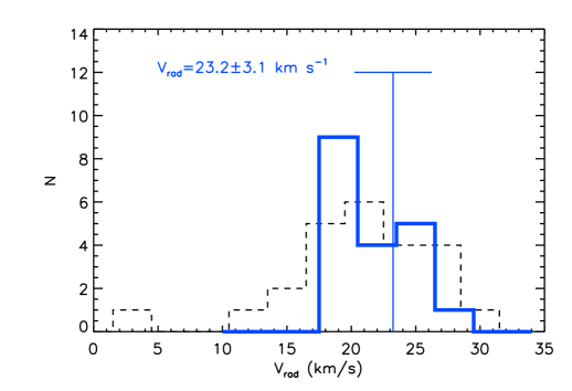
Figure 9: Average RV distribution of the L1615/L1616 low-mass stars (thick solid line). The bar indicates the mean RV value and its standard deviation from the average. The dashed line represents the distribution obtained by Alcalá et al. (2004) for 24 stars in L1616.

A.2 Lithium abundance

Lithium equivalent widths ($EW_{\rm Li}$) were measured by direct integration or by Gaussian fit using the IRAF task splot. Errors in $EW_{\rm Li}$ were estimated in the following way: $i)$ when only one spectrum was available, the standard deviation of three $EW_{\rm Li}$ measurements was adopted; $ii)$ when more than one spectrum was gathered, the standard deviation of the measurements on the different spectra was adopted. Typical errors in $EW_{\rm Li}$ are of 1–20 mÅ. Our $EW_{\rm Li}$ measurements are consistent with the values of Gandolfi et al. (2008) within 17 mÅ on the average.

Mean lithium abundances ($\log n{\rm(Li)}$) were estimated from the average $EW_{\rm Li}$ listed in Table On the accretion properties of young stellar objects in the L1615/L1616 cometary cloud and the effective temperature ($T_{\rm eff}$) from Gandolfi et al. (2008), by using the LTE curves-of-growth reported by Pavlenko & Magazzù (1996) for $T_{\rm eff}>4000$ K, and by Palla et al. (2007) for $T_{\rm eff}<4000$ K. The $\log g$ values were derived as explained in Sect. 3. The main source of error in $\log n{\rm(Li)}$ comes from the uncertainty in $T_{\rm eff}$, which is $\Delta T_{\rm eff}\sim 100$ K (Gandolfi et al. 2008). Taking this value and a mean error of 10 mÅ in $EW_{\rm Li}$ into account, we estimated an uncertainty in $\log n{\rm(Li)}$ ranging from $\sim$0.05$-$0.30 dex for cooler stars ($T_{\rm eff}\sim 3000$ K) down to $\sim$0.05$-$0.15 dex for warmer stars ($T_{\rm eff}\sim 5000$ K), depending on the $EW_{\rm Li}$ value. Moreover, the $\log g$ value affects the lithium abundance, in the sense that the lower the surface gravity the higher the lithium abundance, and vice versa. In particular, the difference in $\log n{\rm(Li)}$ may rise to $\sim\pm 0.1$ dex when considering stars with mean values of $EW_{\rm Li}=500$ (mÅ)  and $T_{\rm eff}=4500$ K and assuming $\Delta\log g=\mp 0.15$ dex, which is the mean error derived from the Gandolfi et al. (2008) stellar parameters.

Appendix B $M_{\star}$ and $\dot{M}_{\rm acc}$ as determined from different evolutionary tracks

Gandolfi et al. (2008) have derived the mass of 56 members of L1615/L1616 by comparing the location of each object on the HR diagram with the theoretical PMS evolutionary tracks by Baraffe et al. (1998) and Chabrier et al. (2000) - Ba98+Ch00, D’Antona & Mazzitelli (1997) - DM97, and Palla & Stahler (1999) - PS99, which are available in the mass ranges $0.003M_{\odot}\leq M\leq 1.40M_{\odot}$, $0.017M_{\odot}\leq M\leq 3M_{\odot}$, $0.1M_{\odot}\leq M\leq 6M_{\odot}$, for Ba98+Ch00, DM97, and PS99 models, respectively. The usage of masses computed from different evolutionary tracks allowed us to estimate the model-dependent uncertainties on $\dot{M}_{\rm acc}$ associated with the derived masses.

In Fig. 10, we show the comparison between the masses derived from the three sets of tracks for the accreting objects. The largest residuals are seen when comparing the Ba98+Ch00 and DM97 tracks. Fig. 11 shows the comparisons of the mass accretion rates when calculated using the different evolutionary tracks. It can be seen that the $\log\dot{M}_{\rm acc}$ values are rather independent of the choice of the PMS track. Therefore, it is the model-dependent uncertainty on mass which produces the dispersion in the $\log\dot{M}_{\rm acc}$ vs. $\log M_{\star}$ plot, whereas the $\log\dot{M}_{\rm acc}$ values are practically insensitive to the choice of the evolutionary model.

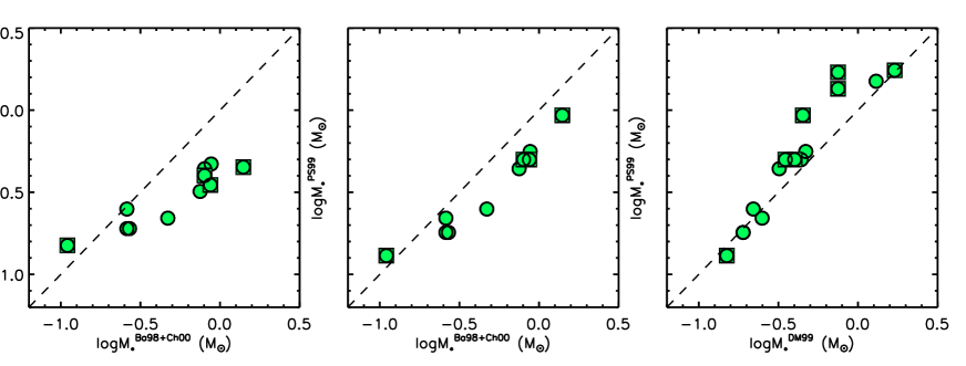
Figure 10: Comparison between masses derived from the Ba98+Ch00 and DM97 tracks (left panel), the Ba98+Ch00 and PS99 tracks (middle panel), and the DM97 and PS99 tracks (right panel) evolutionary tracks. Symbols are as in Fig. 2.

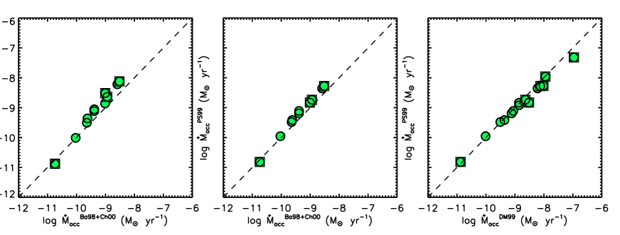
Figure 11: Comparison between mass accretion rates derived using the Ba98+Ch00 and DM97 tracks(left panel), the Ba98+Ch00 and PS99 tracks (middle panel), and the DM97 and PS99 tracks (right panel). Symbols are as in Fig. 2.

Appendix C Notes on individual objects

C.1 TTS 050730.9$-$031846: a sub-luminous YSO with edge-on disk?

The star TTS 050730.9$-$031846 appears to be sub-luminous in the HR diagram reported by Gandolfi et al. (2008), in comparison with typical YSOs in L1615/L1616 of similar effective temperature. Sub-luminous YSOs have been found in other SFRs, like L1630N, L1641, Lupus, and Taurus (see Fang et al. 2009, 2013; Comerón et al. 2003; White & Hillenbrand 2004; Looper et al. 2010; Alcalá et al. 2014). Among the hypotheses to explain the sub-luminosity of these YSOs are the following: $i)$ These YSOs are believed to be embedded or to harbor flared disks with high inclination angles. In this case, the stellar photospheric light and any emission due to physical processes in the inner disk region are severely suppressed by the edge-on disk; $ii)$ Other authors (Baraffe & Chabrier 2010) argue that episodic strong accretion during the PMS evolution produces objects with smaller radius, higher central temperatures, and hence lower luminosity, compared to the non-accreting counterparts of the same age and mass.

The anomalous position of TTS 050730.9$-$031846 on the $J-H$ versus $H-K{\rm s}$ diagram (Fig. 2) would favor the hypothesis of a YSO with a high inclination angle in which both the stellar luminosity and the accretion luminosity are suppressed by the optically thick edge-on disk. A star with the effective temperature of TTS 050730.9$-$031846 ($\sim 3100$ K), at the age of L1615/L1616 ($\sim 3$ Myr; Gandolfi et al. 2008) should have a mass $M_{\star}\sim 0.1\,M_{\odot}$ and should be a factor $\sim 5$ more luminous than observed. This would imply that the mass accretion rate of the star should be a factor (5)^1.5 higher than observed (Alcalá et al. 2014). This means values of $\sim 1.8,1.3,1.4\times 10^{-10}$ $M_{\odot}$ yr^-1 for the masses drawn from the Ba98+Ch00, DM97, PS99 tracks, respectively, i.e. similar to the $\dot{M}_{\rm acc}$ measured in YSOs with the same mass (see Fig. 7).

An edge-on disk may also produce variable circumstellar extinction, inducing changes in the continuum that produce strong variations of the equivalent width of emission lines (see, e.g., the case of the transitional object T Chamaeleontis studied by Schisano et al. 2009). In fact, the $EW_{\rm H\alpha}=-290.00\pm 30.00$ Å of TTS 050730.9$-$031846 measured by Gandolfi et al. (2008) is a factor of about six higher than what we measured here. Whether such strong variability is due to variable circumstellar extinction is not clear, but can only be confirmed by a simultaneous multi-band photometric monitoring of the star.

C.2 TTS 050649.8$-$031933

This star was classified as a WTTs by Gandolfi et al. (2008), but re-analyzing the three spectra acquired by the authors, helium and oxygen lines always appear in emission (as also reported in their Table 4). The results of our three measurements are $EW_{\rm H\alpha}=-15.5,-21.7,-17.6$ Å. Moreover, the $WISE$ colors of the star are consistent with those of a Class II YSO. We thus classify TTS 050649.8$-$031933 as an accreting YSO.

C.3 TTS 050649.8$-$032104 and L1616 MIR 4

Besides the sub-luminous object discussed above, these are the other two YSOs in our sample with the strongest variations in the H$\alpha$ line (see Fig. 1). In particular, for TTS 050649.8$-$032104 Gandolfi et al. (2008) measured $EW_{\rm H\alpha}=-195\pm 5$ Å, i.e. about three times higher than what we measure here, implying a difference of $\sim 0.6$ dex in $\log\dot{M}_{\rm acc}$. In the case of L1616 MIR 4, the Gandolfi et al. (2008) result ($EW_{\rm H\alpha}=-60\pm 6$ Å), is also about three times higher than our measurements, corresponding to a difference of $\sim 0.4$ dex in $\log\dot{M}_{\rm acc}$.

C.4 TTS 050713.5$-$031722

This star was classified as a CTTs by Gandolfi et al. (2008), but re-analyzing their spectrum (see their Table 4), neither helium nor oxygen lines appear in emission (as reported by the authors) and we measured an H$\alpha$ equivalent width of $\sim-8$ Å. Considering its spectral type (K8.5), it can be classified as non-accretor according to the White & Basri (2003) criteria.

C.5 Other targets

In some of the $WISE/2MASS$ color-color diagrams of Fig. 3, the targets TTS 050647.5$-$031910, TTS 050706.2$-$031703, TTS 050752.0$-$032003, 1RXS J051011.5$-$025355, TTS 050734.8$-$031521, and TTS 050729.8$-$031705 appear to be close to or within the regions of Class II objects, according to Koenig et al. (2012). We indeed classified these 6 objects as non-accretors (see Table On the accretion properties of young stellar objects in the L1615/L1616 cometary cloud), because their H$\alpha$ equivalent widths and spectral types are consistent with this object class, according to the White & Basri (2003) criteria.