On the pathwise approximation of stochastic differential equations

Abstract

We consider one-step methods for integrating stochastic differential equations and prove pathwise convergence using ideas from rough path theory. In contrast to alternative theories of pathwise convergence, no knowledge is required of convergence in $p$th mean and the analysis starts from a pathwise bound on the sum of the truncation errors. We show how the theory is applied to the Euler–Maruyama method with fixed and adaptive time-stepping strategies. The assumption on the truncation errors suggests an error-control strategy and we implement this as an adaptive time-stepping Euler–Maruyama method using bounded diffusions. We prove the adaptive method converges and show some computational experiments.

1 Introduction

Let $(\Omega,\mathcal{F},\mathcal{F}_{t},\mathbb{P})$ be a filtered probability space and consider independent $\mathcal{F}_{t}$-Brownian motions $W^{j}(t)$ for $j=1,\dots,m$. We study the following Itô stochastic differential equation (SDE) in ^d:

$$d{y}(t)={g}_{0}({y}(t))\,dt+\sum_{j=1}^{m}{g}_{j}({y}(t))\,dW^{j}(t)$$ (1.1)

where ${g}_{j}\colon{}^{d}\to{}^{d}$ for $j=0,\dots,m$. We assume that ${g}_{j}$ are sufficiently regular and there exists a stochastic process ${y}(t)$ that satisfies this equation on a time interval $[0,T]$ and, if an initial condition is specified, the solution is unique (in the pathwise sense). We denote by ${y}(t;s,{z})$ the solution of Eq. 1.1 for $t\in[s,T]$ with initial condition ${y}(s)={z}\in{}^{d}$. In general, exact solutions ${y}(t)$ are not known and numerical integrators are required to determine quantities of interest, such as averages, sample paths, or exit times. In this paper, we look at one-step methods for approximating sample paths of ${y}(t)$ and analyse the pathwise error using techniques from rough path theory (Davie,, 2007; Friz & Victoir,, 2010). In dynamical system, we are often interested in how sample paths of SDEs change with model parameters and it is important to compute sample paths reliably. The main result is Theorem 3.5. It gives pathwise convergence of the one-step method at a polynomial rate subject to a regularity condition on the sample paths (Assumptions 2.5 and 3.1) and a bound on the sum of the truncation errors (Assumption 3.2). As well as identifying the rate of convergence in terms of the bound on the truncation-error sum, we identify the constant explicitly in terms of those appearing in the assumptions.

Pathwise error analysis is normally performed (Gyöngy,, 1998; Kloeden & Neuenkirch,, 2007) by showing the $p$th mean error converges at a polynomial rate and applying the Borel–Cantelli lemma. Theorem 3.5 predicts the same rates of convergence, for example, for the fixed time-stepping Euler–Maruyama or Milstein method. However, it does not use $p$th mean error estimates.

We take particular interest in the so called bounded-diffusion time-stepping strategy of (Milstein & Tretyakov,, 1999). Instead of taking uniformly spaced times and sampling the Brownian increments from the Gaussian distribution, we choose random times such that the Brownian increment is bounded. Specifically, we define a cuboid $[0,a_{0}]\times[-a_{1},a_{1}]\times\dots\times[-a_{m},a_{m}]$ and choose the first exit time $\tau$ of the process $(t,W^{1}(t),\dots,W^{m}(t))$ from the cuboid. This defines a stopping time $\tau$ and associated exit points $W^{i}(\tau)$ that can be used for the time step and Brownian increments in a numerical integrator for Eq. 1.1. We will use the convergence criterion developed for Theorem 3.5 to choose $a_{i}$ adaptively and thereby implement an error-control strategy for the Euler–Maruyama method. The adaptivity leads to an improvement in the constant in the theoretical error bound, compared to fixed time-stepping. The constant depends on the inherent exponential divergence of sample paths of the SDE with different initial data (see Assumption 3.1) and the constant in the local truncation error (see Assumption 3.2). The adaptive strategy is able to control the second source of error, not the first.

The paper is organised as follows. Section 2 gives background on the time-stepping methods of interest. Working pathwise from the start, Section 3 provides the statement and proof of the main result Theorem 3.5. In Section 4, we give preliminary lemmas that provide pathwise bounds on the sum of the truncation errors, which help in establishing Assumption 3.2, and show that the pathwise-convergence theorem applies to the Euler–Maruyama method with fixed time-steps. In Section 5, we introduce two adaptive time-stepping strategies based on bounded diffusions and present convergence theory and numerical experiments. An appendix reviews some useful results.

2 Background

Our pathwise convergence theory applies to one-step methods for Eq. 1.1 in the case of variable and random time-steps. We work on the time interval $[0,T]$ and consider partitions $\mathcal{T}$ of $[0,T]$.

Definition 2.1 (partitions).

Let $\mathcal{T}$ denote the set of partitions $0=\tau_{0}<\tau_{1}<\dots<\tau_{N}=T$ consisting of $[0,T]$-valued random variables. Let $\mathcal{T}_{\operatorname{stop}}$ be the subset of $\mathcal{T}$ consisting of stopping times (i.e., if $(\tau_{0},\dots,\tau_{N})\in\mathcal{T}_{\operatorname{stop}}$ then $\tau_{j}$ is $\mathcal{F}_{\tau_{j}}$-measurable for $j=0,\dots,N$). Let ${\hat{s\mkern 2.0mu}\mkern-2.0mu}{}=\tau_{n}$ if $\tau_{n}\leq s<\tau_{n+1}$.

We generate approximations ${y}_{k}=S_{0k}(z)$ to ${y}(\tau_{k};\tau_{0},{z})$ at times $\tau_{k}$ in a partition $(\tau_{0},\dots,\tau_{n})\in\mathcal{T}$ using one-step methods.

Definition 2.2 (one-step method).

Given $\tau_{n}<\tau_{n+1}$, a one-step method ${S}_{n,n+1}$ is a map from ^d to the set of ^d-valued random variables. For a given partition $\mathcal{T}$ and $0\leq k<n\leq N$, we use the notation ${S}((\tau_{k},\dots,\tau_{n}),{z})$ or the abbreviation ${S}_{kn}({z})$ to denote ${S}_{n-1,n}\circ\dots\circ{S}_{k,k+1}({z})$, the action of applying the one-step method successively over the time steps $[\tau_{k},\tau_{k+1}],\dots,[\tau_{n-1},\tau_{n}]$.

The simplest useful example is the Euler–Maruyama method with fixed time-step $h$ given by ${S}_{n,n+1}({y}_{n})={y}_{n+1}$ for times $\tau_{n}=\tau_{0}+nh$ and

$${y}_{n+1}={y}_{n}+{g}_{0}({y}_{n})(\tau_{n+1}-\tau_{n})+\sum_{j=1}^{m}{g}_{j}({y}_{n})\left(\mathchoice{\raisebox{0.0pt}{$\displaystyle{\vphantom{\bigm{|}}\mathopen{}W^{j}(\tau_{n+1})-W^{j}(\tau_{n})}$}}{W^{j}(\tau_{n+1})-W^{j}(\tau_{n})}{W^{j}(\tau_{n+1})-W^{j}(\tau_{n})}{W^{j}(\tau_{n+1})-W^{j}(\tau_{n})}\right).$$ (2.1)

The implicit Euler–Maruyama method, given by

$${y}_{n+1}={y}_{n}+{g}_{0}({y}_{n+1})(\tau_{n+1}-\tau_{n})+\sum_{j=1}^{m}{g}_{j}({y}_{n})\left(\mathchoice{\raisebox{0.0pt}{$\displaystyle{\vphantom{\bigm{|}}\mathopen{}W^{j}(\tau_{n+1})-W^{j}(\tau_{n})}$}}{W^{j}(\tau_{n+1})-W^{j}(\tau_{n})}{W^{j}(\tau_{n+1})-W^{j}(\tau_{n})}{W^{j}(\tau_{n+1})-W^{j}(\tau_{n})}\right),$$ (2.2)

is included if the nonlinear equations can be solved for any $y_{n}$ to define $y_{n+1}$ uniquely. We will introduce an example of random times $\tau_{n}$ in Section 5.

Key to the analysis of convergence of one-step methods is the local truncation error.

Definition 2.3 (local truncation error).

For $\tau_{n}<\tau_{n+1}$, the local truncation error at ${z}\in{}^{d}$ of a one-step method $S_{n,n+1}(z)$ is

$${\delta}(\tau_{n},\tau_{n+1},{z})\coloneq{y}(\tau_{n+1};\tau_{n},{z})-{S}_{n,n+1}({z}).$$ (2.3)

For the Euler–Maruyama method, writing $dW^{0}(t)=dt$, the local truncation error is

$$\begin{split}\delta(\tau_{k},\tau_{k+1},z)=&\sum_{i,j=0}^{m}\int_{\tau_{k}}^{\tau_{k+1}}\int_{\tau_{k}}^{s}q_{ij}\left(\mathchoice{\raisebox{0.0pt}{$\displaystyle{\vphantom{\bigm{|}}\mathopen{}y(r;\tau_{k},z)}$}}{y(r;\tau_{k},z)}{y(r;\tau_{k},z)}{y(r;\tau_{k},z)}\right)\,dW^{i}(r)\,dW^{j}(s),\end{split}$$ (2.4)

where

$$q_{ij}(y)\coloneq\begin{cases}\displaystyle Dg_{j}(y)g_{0}(y)+\frac{1}{2}\sum_{k=1}^{m}D^{2}g_{j}(y)(g_{k}(y),g_{k}(y)),&i=0,\\ Dg_{j}(y)g_{i}(y),&i\neq 0.\end{cases}$$ (2.5)

See for example (Kloeden & Platen,, 1992; Milstein,, 1995). Under regularity assumptions on $g_{j}$, we can estimate the $p$th moment by using the Burkholder–Davis–Gundy inequality and find $\mathbb{E}\left[\mathchoice{\raisebox{0.0pt}{$\displaystyle{\vphantom{\bigm{|}}\mathopen{}\left\|\mathchoice{\raisebox{0.0pt}{$\displaystyle{\vphantom{\bigm{|}}\mathopen{}\delta}$}}{\smash{\delta}}{\delta}{\delta}\right\|^{p}}$}}{\left\|\mathchoice{\raisebox{0.0pt}{$\displaystyle{\vphantom{\bigm{|}}\mathopen{}\delta}$}}{\smash{\delta}}{\delta}{\delta}\right\|^{p}}{\left\|\mathchoice{\raisebox{0.0pt}{$\displaystyle{\vphantom{\bigm{|}}\mathopen{}\delta}$}}{\smash{\delta}}{\delta}{\delta}\right\|^{p}}{\left\|\mathchoice{\raisebox{0.0pt}{$\displaystyle{\vphantom{\bigm{|}}\mathopen{}\delta}$}}{\smash{\delta}}{\delta}{\delta}\right\|^{p}}\right]=\mathcal{O}\left(\mathchoice{\raisebox{0.0pt}{$\displaystyle{\vphantom{\bigm{|}}\mathopen{}h^{p}}$}}{h^{p}}{h^{p}}{h^{p}}\right)$ for $p\geq 2$ and then show that the local truncation error $\delta(\tau_{k},\tau_{k+1},z)=\mathcal{O}\left(\mathchoice{\raisebox{0.0pt}{$\displaystyle{\vphantom{\bigm{|}}\mathopen{}h^{\gamma+1/2-\epsilon}}$}}{h^{\gamma+1/2-\epsilon}}{h^{\gamma+1/2-\epsilon}}{h^{\gamma+1/2-\epsilon}}\right)$ with $\gamma=1/2$ and $\epsilon>0$. Note the use of $\epsilon$ in writing the condition on the truncation error, similar to saying Brownian motion is Hölder continuous with exponent $1/2-\epsilon$, any $\epsilon>0$. We make the following assumption on the truncation error.

Assumption 2.4.

For a partition $(\tau_{0},\dots,\tau_{N})\in\mathcal{T}$, an $\epsilon\in(0,1)$, and a random variable $K_{\operatorname{TE}}>0$, it holds that

$$\left\|\mathchoice{\raisebox{0.0pt}{$\displaystyle{\vphantom{\bigm{|}}\mathopen{}{\delta}(\tau_{k},\tau_{k+1},{z})}$}}{\smash{{\delta}(\tau_{k},\tau_{k+1},{z})}}{{\delta}(\tau_{k},\tau_{k+1},{z})}{{\delta}(\tau_{k},\tau_{k+1},{z})}\right\|\leq K_{\operatorname{TE}}|\tau_{k+1}-\tau_{k}|^{\gamma+1/2-\epsilon},\qquad\text{ $\forall{z}\in{}^{d}$, $k=0,\dots,N-1$.}$$ (2.6)

In general, we want to refine the partition $\mathcal{T}$ and keep $K_{\operatorname{TE}}$ and $\epsilon$ constant in Eq. 2.6, in which case $\gamma$ indicates the pathwise order of convergence with respect to the mesh width $h\coloneq\max_{k}|\tau_{k+1}-\tau_{k}|$ (as we show in Theorem 3.5). We will denote such methods by ${S}^{\gamma}_{kn}$. Before Theorem 3.5, we review a simpler result from (Gaines & Lyons,, 1997) that gives order $\gamma-1/2$ convergence. We assume the following continuity with respect to initial data property, which is satisfied by $y(t;s,z)$ if $g_{j}\in\mathrm{C}_{\mathrm{b}}^{3}({}^{d},{}^{d})$ (Friz & Victoir,, 2010, Theorem 10.26). Here, $C_{\mathrm{b}}^{r}({}^{d},{}^{d})$ is the set of functions $g\colon{}^{d}\to{}^{d}$ with $r\in\mathbb{N}$ uniformly bounded and continuous derivatives and norm $\left\|\mathchoice{\raisebox{0.0pt}{$\displaystyle{\vphantom{\bigm{|}}\mathopen{}g}$}}{\smash{g}}{g}{g}\right\|_{C_{\mathrm{b}}^{r}}\coloneq\sup_{|\alpha|\leq r}\sup_{{x}\in{}^{d}}\left\|\mathchoice{\raisebox{0.0pt}{$\displaystyle{\vphantom{\bigm{|}}\mathopen{}D^{\alpha}g({x})}$}}{\smash{D^{\alpha}g({x})}}{D^{\alpha}g({x})}{D^{\alpha}g({x})}\right\|$.

Assumption 2.5.

For a random variable $L_{\operatorname{SDE}}>0$,

$$\left\|\mathchoice{\raisebox{0.0pt}{$\displaystyle{\vphantom{\bigm{|}}\mathopen{}{y}(t;s,{z}^{1})-{y}(t;s,{z}^{2})}$}}{\smash{{y}(t;s,{z}^{1})-{y}(t;s,{z}^{2})}}{{y}(t;s,{z}^{1})-{y}(t;s,{z}^{2})}{{y}(t;s,{z}^{1})-{y}(t;s,{z}^{2})}\right\|\leq L_{\operatorname{SDE}}\left\|\mathchoice{\raisebox{0.0pt}{$\displaystyle{\vphantom{\bigm{|}}\mathopen{}{z}^{1}-{z}^{2}}$}}{\smash{{z}^{1}-{z}^{2}}}{{z}^{1}-{z}^{2}}{{z}^{1}-{z}^{2}}\right\|$$ (2.7)

for $0\leq s\leq t\leq T$ and ${z}^{1},{z}^{2}\in{}^{d}$.

We define $h\coloneq\max_{k}|\tau_{k+1}-\tau_{k}|$ and will use $h$ to measure rates of convergence.

Theorem 2.6 (convergence rate $\gamma-1/2$).

Let Assumption 2.5 hold for Eq. 1.1 and Assumption 2.4 hold for ${S}^{\gamma}_{kn}$. Then, for any ${y}_{0}\in{}^{d}$,

$$\max_{n=0,\dots,N}\left\|\mathchoice{\raisebox{0.0pt}{$\displaystyle{\vphantom{\bigm{|}}\mathopen{}{S}^{\gamma}_{0n}({y}_{0})-{y}(\tau_{n};0,{y}_{0})}$}}{\smash{{S}^{\gamma}_{0n}({y}_{0})-{y}(\tau_{n};0,{y}_{0})}}{{S}^{\gamma}_{0n}({y}_{0})-{y}(\tau_{n};0,{y}_{0})}{{S}^{\gamma}_{0n}({y}_{0})-{y}(\tau_{n};0,{y}_{0})}\right\|\leq L_{\operatorname{SDE}}\,K_{\operatorname{TE}}\,T\,h^{\gamma-\epsilon-1/2},$$

where $\epsilon$, $K_{\operatorname{TE}}$, and $L_{\operatorname{SDE}}$ are given in Eqs. 2.7 and 2.6.

Proof.

Let ${{y}}_{n}\coloneq{S}_{0n}^{\gamma}({y}_{0})$ and let ${y}^{k}(t)\coloneq{y}(t;\tau_{k},{{y}}_{k})$ for $t\in[\tau_{k},T]$. Then,

$$\left\|\mathchoice{\raisebox{0.0pt}{$\displaystyle{\vphantom{\bigm{|}}\mathopen{}{y}^{k}(\tau_{k+1})-{{y}}_{k+1}}$}}{\smash{{y}^{k}(\tau_{k+1})-{{y}}_{k+1}}}{{y}^{k}(\tau_{k+1})-{{y}}_{k+1}}{{y}^{k}(\tau_{k+1})-{{y}}_{k+1}}\right\|=\left\|\mathchoice{\raisebox{0.0pt}{$\displaystyle{\vphantom{\bigm{|}}\mathopen{}{y}(\tau_{k+1};\tau_{k},{{y}}_{k})-{S}^{\gamma}_{k,k+1}({{y}}_{k})}$}}{\smash{{y}(\tau_{k+1};\tau_{k},{{y}}_{k})-{S}^{\gamma}_{k,k+1}({{y}}_{k})}}{{y}(\tau_{k+1};\tau_{k},{{y}}_{k})-{S}^{\gamma}_{k,k+1}({{y}}_{k})}{{y}(\tau_{k+1};\tau_{k},{{y}}_{k})-{S}^{\gamma}_{k,k+1}({{y}}_{k})}\right\|.$$

By Definition 2.3, this is bounded by $K_{\operatorname{TE}}|\tau_{k+1}-\tau_{k}|^{\gamma+1/2-\epsilon}$. By Assumption 2.5,

$$\left\|\mathchoice{\raisebox{0.0pt}{$\displaystyle{\vphantom{\bigm{|}}\mathopen{}{y}^{k}(\tau_{n})-{y}^{k+1}(\tau_{n})}$}}{\smash{{y}^{k}(\tau_{n})-{y}^{k+1}(\tau_{n})}}{{y}^{k}(\tau_{n})-{y}^{k+1}(\tau_{n})}{{y}^{k}(\tau_{n})-{y}^{k+1}(\tau_{n})}\right\| \leq L_{\operatorname{SDE}}\left\|\mathchoice{\raisebox{0.0pt}{$\displaystyle{\vphantom{\bigm{|}}\mathopen{}{y}^{k}(\tau_{k+1})-{y}^{k+1}(\tau_{k+1})}$}}{\smash{{y}^{k}(\tau_{k+1})-{y}^{k+1}(\tau_{k+1})}}{{y}^{k}(\tau_{k+1})-{y}^{k+1}(\tau_{k+1})}{{y}^{k}(\tau_{k+1})-{y}^{k+1}(\tau_{k+1})}\right\|=L_{\operatorname{SDE}}\left\|\mathchoice{\raisebox{0.0pt}{$\displaystyle{\vphantom{\bigm{|}}\mathopen{}{y}^{k}(\tau_{k+1})-{{y}}_{k+1}}$}}{\smash{{y}^{k}(\tau_{k+1})-{{y}}_{k+1}}}{{y}^{k}(\tau_{k+1})-{{y}}_{k+1}}{{y}^{k}(\tau_{k+1})-{{y}}_{k+1}}\right\|$$

$$\leq L_{\operatorname{SDE}}\left(\mathchoice{\raisebox{0.0pt}{$\displaystyle{\vphantom{\bigm{|}}\mathopen{}K_{\operatorname{TE}}|\tau_{k+1}-\tau_{k}|^{\gamma-\epsilon+1/2}}$}}{K_{\operatorname{TE}}|\tau_{k+1}-\tau_{k}|^{\gamma-\epsilon+1/2}}{K_{\operatorname{TE}}|\tau_{k+1}-\tau_{k}|^{\gamma-\epsilon+1/2}}{K_{\operatorname{TE}}|\tau_{k+1}-\tau_{k}|^{\gamma-\epsilon+1/2}}\right).$$

If we now sum over $k=0,\dots,n-1$, the triangle inequality applies and we obtain

$$\left\|\mathchoice{\raisebox{0.0pt}{$\displaystyle{\vphantom{\bigm{|}}\mathopen{}{y}(\tau_{n};0,{y}_{0})-{S}^{\gamma}_{0n}({y}_{0})}$}}{\smash{{y}(\tau_{n};0,{y}_{0})-{S}^{\gamma}_{0n}({y}_{0})}}{{y}(\tau_{n};0,{y}_{0})-{S}^{\gamma}_{0n}({y}_{0})}{{y}(\tau_{n};0,{y}_{0})-{S}^{\gamma}_{0n}({y}_{0})}\right\|=\left\|\mathchoice{\raisebox{0.0pt}{$\displaystyle{\vphantom{\bigm{|}}\mathopen{}{y}^{0}(\tau_{n})-{y}^{n}(\tau_{n})}$}}{\smash{{y}^{0}(\tau_{n})-{y}^{n}(\tau_{n})}}{{y}^{0}(\tau_{n})-{y}^{n}(\tau_{n})}{{y}^{0}(\tau_{n})-{y}^{n}(\tau_{n})}\right\|\leq L_{\operatorname{SDE}}\,K_{\operatorname{TE}}\sum_{k=0}^{n-1}\left|\mathchoice{\raisebox{0.0pt}{$\displaystyle{\vphantom{\bigm{|}}\mathopen{}\tau_{k+1}-\tau_{k}}$}}{\smash{\tau_{k+1}-\tau_{k}}}{\tau_{k+1}-\tau_{k}}{\tau_{k+1}-\tau_{k}}\right|^{\gamma-\epsilon+1/2},$$

since ${y}^{0}(\tau_{n})={y}(\tau_{n};0,{y}_{0})$ and ${y}^{n}(\tau_{n})={S}^{\gamma}_{0n}({y}_{0})$. Finally, $\tau_{n}\leq T$, so that

$$\left\|\mathchoice{\raisebox{0.0pt}{$\displaystyle{\vphantom{\bigm{|}}\mathopen{}{y}(\tau_{n};0,{y}_{0})-{S}^{\gamma}_{0n}({y}_{0})}$}}{\smash{{y}(\tau_{n};0,{y}_{0})-{S}^{\gamma}_{0n}({y}_{0})}}{{y}(\tau_{n};0,{y}_{0})-{S}^{\gamma}_{0n}({y}_{0})}{{y}(\tau_{n};0,{y}_{0})-{S}^{\gamma}_{0n}({y}_{0})}\right\|\leq L_{\operatorname{SDE}}\,K_{\operatorname{TE}}\,T\,h^{\gamma-\epsilon-1/2}.$$

∎

Suppose that $\mathcal{T}_{h}$ is a family of partitions with $h=\max_{k}\left|\mathchoice{\raisebox{0.0pt}{$\displaystyle{\vphantom{\bigm{|}}\mathopen{}\tau_{k+1}-\tau_{k}}$}}{\smash{\tau_{k+1}-\tau_{k}}}{\tau_{k+1}-\tau_{k}}{\tau_{k+1}-\tau_{k}}\right|$ for $(\tau_{0},\dots,\tau_{N})\in\mathcal{T}_{h}$. When Assumption 2.5 holds with the same $K_{\operatorname{TE}}$ for each $\mathcal{T}_{h}$, this theorem provides convergence of the numerical approximation $S^{\gamma}_{0n}(y_{0})$ on the partition $\mathcal{T}_{h}$ to the true solution in the pathwise sense in the limit $h\to 0$ and the pathwise error is $\mathcal{O}\left(\mathchoice{\raisebox{0.0pt}{$\displaystyle{\vphantom{\bigm{|}}\mathopen{}h^{\gamma-\epsilon-1/2}}$}}{h^{\gamma-\epsilon-1/2}}{h^{\gamma-\epsilon-1/2}}{h^{\gamma-\epsilon-1/2}}\right)$, for $\epsilon>0$. The conditions are general (e.g., allowing time steps that are not uniformly spaced or are not stopping times). However the theorem does not imply convergence of the Euler–Maruyama method and is not optimal for the Milstein method where the error is $\mathcal{O}\left(\mathchoice{\raisebox{0.0pt}{$\displaystyle{\vphantom{\bigm{|}}\mathopen{}h^{1-\epsilon}}$}}{h^{1-\epsilon}}{h^{1-\epsilon}}{h^{1-\epsilon}}\right)$ not $\mathcal{O}\left(\mathchoice{\raisebox{0.0pt}{$\displaystyle{\vphantom{\bigm{|}}\mathopen{}h^{1/2-\epsilon}}$}}{h^{1/2-\epsilon}}{h^{1/2-\epsilon}}{h^{1/2-\epsilon}}\right)$ for fixed time-steps.

3 Main result on pathwise convergence

To achieve a rate of convergence higher than the rate in Theorem 2.6, we introduce two more assumptions. The first like Assumption 2.5 concerns the solution of the SDE itself. Again, the condition holds if $g_{j}\in\mathrm{C}_{\mathrm{b}}^{3}({}^{d},{}^{d})$ (see Lemma A.1).

Assumption 3.1.

For an $0<\epsilon<1/2$ and a random variable $K_{\operatorname{SDE}}>0$,

$$\left\|\mathchoice{\raisebox{0.0pt}{$\displaystyle{\vphantom{\bigm{|}}\mathopen{}\left(\mathchoice{\raisebox{0.0pt}{$\displaystyle{\vphantom{\bigm{|}}\mathopen{}{y}(t;s,{z}^{1})-{z}^{1}}$}}{{y}(t;s,{z}^{1})-{z}^{1}}{{y}(t;s,{z}^{1})-{z}^{1}}{{y}(t;s,{z}^{1})-{z}^{1}}\right)-\left(\mathchoice{\raisebox{0.0pt}{$\displaystyle{\vphantom{\bigm{|}}\mathopen{}{y}(t;s,{z}^{2})-{z}^{2}}$}}{{y}(t;s,{z}^{2})-{z}^{2}}{{y}(t;s,{z}^{2})-{z}^{2}}{{y}(t;s,{z}^{2})-{z}^{2}}\right)}$}}{\smash{\left(\mathchoice{\raisebox{0.0pt}{$\displaystyle{\vphantom{\bigm{|}}\mathopen{}{y}(t;s,{z}^{1})-{z}^{1}}$}}{{y}(t;s,{z}^{1})-{z}^{1}}{{y}(t;s,{z}^{1})-{z}^{1}}{{y}(t;s,{z}^{1})-{z}^{1}}\right)-\left(\mathchoice{\raisebox{0.0pt}{$\displaystyle{\vphantom{\bigm{|}}\mathopen{}{y}(t;s,{z}^{2})-{z}^{2}}$}}{{y}(t;s,{z}^{2})-{z}^{2}}{{y}(t;s,{z}^{2})-{z}^{2}}{{y}(t;s,{z}^{2})-{z}^{2}}\right)}}{\left(\mathchoice{\raisebox{0.0pt}{$\displaystyle{\vphantom{\bigm{|}}\mathopen{}{y}(t;s,{z}^{1})-{z}^{1}}$}}{{y}(t;s,{z}^{1})-{z}^{1}}{{y}(t;s,{z}^{1})-{z}^{1}}{{y}(t;s,{z}^{1})-{z}^{1}}\right)-\left(\mathchoice{\raisebox{0.0pt}{$\displaystyle{\vphantom{\bigm{|}}\mathopen{}{y}(t;s,{z}^{2})-{z}^{2}}$}}{{y}(t;s,{z}^{2})-{z}^{2}}{{y}(t;s,{z}^{2})-{z}^{2}}{{y}(t;s,{z}^{2})-{z}^{2}}\right)}{\left(\mathchoice{\raisebox{0.0pt}{$\displaystyle{\vphantom{\bigm{|}}\mathopen{}{y}(t;s,{z}^{1})-{z}^{1}}$}}{{y}(t;s,{z}^{1})-{z}^{1}}{{y}(t;s,{z}^{1})-{z}^{1}}{{y}(t;s,{z}^{1})-{z}^{1}}\right)-\left(\mathchoice{\raisebox{0.0pt}{$\displaystyle{\vphantom{\bigm{|}}\mathopen{}{y}(t;s,{z}^{2})-{z}^{2}}$}}{{y}(t;s,{z}^{2})-{z}^{2}}{{y}(t;s,{z}^{2})-{z}^{2}}{{y}(t;s,{z}^{2})-{z}^{2}}\right)}\right\| \leq K_{\operatorname{SDE}}(t-s)^{1/2-\epsilon/3}\left\|\mathchoice{\raisebox{0.0pt}{$\displaystyle{\vphantom{\bigm{|}}\mathopen{}{z}^{1}-{z}^{2}}$}}{\smash{{z}^{1}-{z}^{2}}}{{z}^{1}-{z}^{2}}{{z}^{1}-{z}^{2}}\right\|,$$ (3.1)

for all $0\leq s<t\leq T$ and ${z}^{1},{z}^{2}\in{}^{d}$.

The second assumption is a pathwise version of the independent-increment property of Brownian motion and sets a bound on the sum of truncation errors along each path. We will verify this assumption in the case $(\tau_{0},\dots,\tau_{N})\in{\cal T}_{\operatorname{stop}}\subset{\cal T}$, so that the $\tau_{j}$ are stopping times. Indeed, (Gaines & Lyons,, 1997) provides an example of a time-stepping strategy where the Euler–Maruyama method fails when $\tau_{j}$ are not adapted. Consider an integrator ${S}^{\gamma}_{kn}$ with respect to $(\tau_{0},\dots,\tau_{N})\in\mathcal{T}$ and recall $h\coloneq\max_{k=0,\dots,N-1}|\tau_{k+1}-\tau_{k}|$.

Assumption 3.2 (truncation-error sum).

For an initial condition $y_{0}\in{}^{d}$, an $\epsilon\in(0,1/2)$, and random variable $K_{\operatorname{TES}}>0$, it holds that

$$\left\|\mathchoice{\raisebox{0.0pt}{$\displaystyle{\vphantom{\bigm{|}}\mathopen{}{X}_{kn}({y}_{0})}$}}{\smash{{X}_{kn}({y}_{0})}}{{X}_{kn}({y}_{0})}{{X}_{kn}({y}_{0})}\right\|\leq K_{\operatorname{TES}}(\tau_{n}-\tau_{k})^{(1+\epsilon)/2}h^{\gamma-\epsilon},\quad 0\leq k<n\leq N,$$ (3.2)

where ${X}_{kn}(y_{0})\coloneq\sum_{j=k}^{n-1}{\delta}(\tau_{j},\tau_{j+1},{y}_{j})$ and ${y}_{n}={S}_{0n}^{\gamma}({y}_{0})$.

In general, we want to refine the partition $\mathcal{T}$ and take limits as $h\downarrow 0$ while keeping $K_{\operatorname{TES}}$ and $\epsilon$ constant.

For the Euler–Maruyama method (2.1) with fixed time-step $\tau_{n+1}-\tau_{n}=h$, Eq. 3.2 follows because

$$X_{kn}(y_{0})=X(\tau_{k},\tau_{n}),\quad\text{ for }X(r,t)\coloneq\sum_{i,j=0}^{m}\int_{r}^{t}\int_{{\hat{s\mkern 2.0mu}\mkern-2.0mu}{}}^{s}q_{ij}\left(\mathchoice{\raisebox{0.0pt}{$\displaystyle{\vphantom{\bigm{|}}\mathopen{}y(r;{\hat{r\mkern 2.0mu}\mkern-2.0mu}{},{\hat{y\mkern 1.0mu}\mkern-1.0mu}{}(r))}$}}{y(r;{\hat{r\mkern 2.0mu}\mkern-2.0mu}{},{\hat{y\mkern 1.0mu}\mkern-1.0mu}{}(r))}{y(r;{\hat{r\mkern 2.0mu}\mkern-2.0mu}{},{\hat{y\mkern 1.0mu}\mkern-1.0mu}{}(r))}{y(r;{\hat{r\mkern 2.0mu}\mkern-2.0mu}{},{\hat{y\mkern 1.0mu}\mkern-1.0mu}{}(r))}\right)\,dW^{i}(r)\,dW^{j}(s),$$

by writing Eqs. 2.4 and 2.5 with the notation ${\hat{y\mkern 1.0mu}\mkern-1.0mu}{}(r)\coloneq y_{n}$ for $\tau_{n}\leq r<\tau_{n+1}$. Then, if the $q_{ij}$ are well-behaved, we can show that $\mathbb{E}\left[\mathchoice{\raisebox{0.0pt}{$\displaystyle{\vphantom{\bigm{|}}\mathopen{}\left\|\mathchoice{\raisebox{0.0pt}{$\displaystyle{\vphantom{\bigm{|}}\mathopen{}X(r,t)}$}}{\smash{X(r,t)}}{X(r,t)}{X(r,t)}\right\|^{p}}$}}{\left\|\mathchoice{\raisebox{0.0pt}{$\displaystyle{\vphantom{\bigm{|}}\mathopen{}X(r,t)}$}}{\smash{X(r,t)}}{X(r,t)}{X(r,t)}\right\|^{p}}{\left\|\mathchoice{\raisebox{0.0pt}{$\displaystyle{\vphantom{\bigm{|}}\mathopen{}X(r,t)}$}}{\smash{X(r,t)}}{X(r,t)}{X(r,t)}\right\|^{p}}{\left\|\mathchoice{\raisebox{0.0pt}{$\displaystyle{\vphantom{\bigm{|}}\mathopen{}X(r,t)}$}}{\smash{X(r,t)}}{X(r,t)}{X(r,t)}\right\|^{p}}\right]=\mathcal{O}\left(\mathchoice{\raisebox{0.0pt}{$\displaystyle{\vphantom{\bigm{|}}\mathopen{}h^{p/2}(t-r)^{p/2}}$}}{h^{p/2}(t-r)^{p/2}}{h^{p/2}(t-r)^{p/2}}{h^{p/2}(t-r)^{p/2}}\right)$ and we expect that $\left\|\mathchoice{\raisebox{0.0pt}{$\displaystyle{\vphantom{\bigm{|}}\mathopen{}X_{kn}(y_{0})}$}}{\smash{X_{kn}(y_{0})}}{X_{kn}(y_{0})}{X_{kn}(y_{0})}\right\|\leq K_{\operatorname{TES}}(\tau_{n}-\tau_{k})^{(1/2-\epsilon/4)}h^{1/2-\epsilon/4}$ for some $K_{\operatorname{TES}}>0$ independent of $h$. A further manipulation using $|\tau_{n}-\tau_{k}|\geq h$ then yields Eq. 3.2 with $\gamma=1/2$. Thus, there are two steps to verifying Eq. 3.2: first, derive pathwise estimates of certain stochastic integrals and, second, show that the time step $\tau_{j+1}-\tau_{j}$ is not too small relative to $h$. We verify Assumption 3.2 for the Euler–Maruyama method with different time-stepping methods in the proofs of Theorem 4.2 (fixed time-stepping) and Theorems 5.2 and 5.4 (adaptive bounded diffusions).

3.1 Preliminary lemma

Before giving the main convergence result in Theorem 3.5, we give two lemmas required for its proof. The following result plays the role normally assumed by Gronwall’s inequality in proving Theorem 3.5: the local truncation error will determine $C_{2}$ and the $J_{kn}$ is one of two terms that control the global error $y_{n}-y(\tau_{n};\tau_{k},y_{k})$. Then, (3.3) describes how the local truncation error affects the global error. We derive (3.4), which shows $J_{kn}$ is proportional to $L$ and hence $C_{2}$. That is, roughly, the local truncation error $C_{2}$ controls the global error $J_{kn}$. The result is adapted from (Davie,, 2007).

Lemma 3.3.

For a sequence $0=t_{0}<t_{1}<t_{2}<\cdots$, consider a set of vectors ${J}_{kn}$ indexed by $k,n\in\mathbb{N}$. For constants $C_{1},C_{2},\gamma>0$, $\alpha>1$, suppose that

$$\left\|\mathchoice{\raisebox{0.0pt}{$\displaystyle{\vphantom{\bigm{|}}\mathopen{}{J}_{kn}}$}}{\smash{{J}_{kn}}}{{J}_{kn}}{{J}_{kn}}\right\|\leq\left\|\mathchoice{\raisebox{0.0pt}{$\displaystyle{\vphantom{\bigm{|}}\mathopen{}{J}_{k\ell}}$}}{\smash{{J}_{k\ell}}}{{J}_{k\ell}}{{J}_{k\ell}}\right\|\left[\mathchoice{\raisebox{0.0pt}{$\displaystyle{\vphantom{\bigm{|}}\mathopen{}1+C_{1}|t_{n}-t_{k}|^{\gamma}}$}}{1+C_{1}|t_{n}-t_{k}|^{\gamma}}{1+C_{1}|t_{n}-t_{k}|^{\gamma}}{1+C_{1}|t_{n}-t_{k}|^{\gamma}}\right]+\left\|\mathchoice{\raisebox{0.0pt}{$\displaystyle{\vphantom{\bigm{|}}\mathopen{}{J}_{\ell+1,n}}$}}{\smash{{J}_{\ell+1,n}}}{{J}_{\ell+1,n}}{{J}_{\ell+1,n}}\right\|+C_{2}|t_{n}-t_{k}|^{\alpha}$$ (3.3)

if $|t_{k}-t_{\ell}|\leq\frac{1}{2}|t_{n}-t_{k}|$ and $|t_{\ell+1}-t_{n}|\leq\tfrac{1}{2}|t_{n}-t_{k}|$ and that

$${J}_{kk}={0},\qquad\left\|\mathchoice{\raisebox{0.0pt}{$\displaystyle{\vphantom{\bigm{|}}\mathopen{}{J}_{k,k+1}}$}}{\smash{{J}_{k,k+1}}}{{J}_{k,k+1}}{{J}_{k,k+1}}\right\|\leq L|t_{k+1}-t_{k}|^{\alpha}\quad\text{for $L\coloneq\dfrac{2C_{2}}{1-2^{1-\alpha}}$.}$$

Then

$$\left\|\mathchoice{\raisebox{0.0pt}{$\displaystyle{\vphantom{\bigm{|}}\mathopen{}{J}_{kn}}$}}{\smash{{J}_{kn}}}{{J}_{kn}}{{J}_{kn}}\right\|\leq L|t_{n}-t_{k}|^{\alpha}\quad\text{if $|t_{n}-t_{k}|\leq\delta$ }$$ (3.4)

for $\delta>0$ such that $2^{1-\alpha}C_{1}\delta^{\gamma}={1-2^{1-\alpha}}$.

Proof.

By the assumption on ${J}_{kk}$ and ${J}_{k,k+1}$, Eq. 3.4 holds for $|k-n|<2$. We complete the proof by induction on $n-k$ by showing Eq. 3.4 given

$$\left\|\mathchoice{\raisebox{0.0pt}{$\displaystyle{\vphantom{\bigm{|}}\mathopen{}{J}_{kn^{\prime}}}$}}{\smash{{J}_{kn^{\prime}}}}{{J}_{kn^{\prime}}}{{J}_{kn^{\prime}}}\right\|\leq L|t_{n^{\prime}}-t_{k}|^{\alpha} k\leq n^{\prime}<n$$  for all . (3.5)

Let $\ell$ be the largest integer satisfying $k\leq\ell<n$ and $|t_{\ell}-t_{k}|\leq\frac{1}{2}|t_{n}-t_{k}|$. Then, also $|t_{n}-t_{\ell+1}|\leq\tfrac{1}{2}|t_{n}-t_{k}|$ and, by Eq. 3.5,

$$\left\|\mathchoice{\raisebox{0.0pt}{$\displaystyle{\vphantom{\bigm{|}}\mathopen{}{J}_{k\ell}}$}}{\smash{{J}_{k\ell}}}{{J}_{k\ell}}{{J}_{k\ell}}\right\|\leq L|t_{\ell}-t_{k}|^{\alpha}\leq L2^{-\alpha}|t_{n}-t_{k}|^{\alpha},\qquad\left\|\mathchoice{\raisebox{0.0pt}{$\displaystyle{\vphantom{\bigm{|}}\mathopen{}{J}_{\ell+1,n}}$}}{\smash{{J}_{\ell+1,n}}}{{J}_{\ell+1,n}}{{J}_{\ell+1,n}}\right\|\leq L|t_{n}-t_{\ell+1}|^{\alpha}\leq L2^{-\alpha}|t_{n}-t_{k}|^{\alpha}.$$

From Eq. 3.3,

$$\left\|\mathchoice{\raisebox{0.0pt}{$\displaystyle{\vphantom{\bigm{|}}\mathopen{}{J}_{kn}}$}}{\smash{{J}_{kn}}}{{J}_{kn}}{{J}_{kn}}\right\| \leq\left\|\mathchoice{\raisebox{0.0pt}{$\displaystyle{\vphantom{\bigm{|}}\mathopen{}{J}_{k\ell}}$}}{\smash{{J}_{k\ell}}}{{J}_{k\ell}}{{J}_{k\ell}}\right\|\left[\mathchoice{\raisebox{0.0pt}{$\displaystyle{\vphantom{\bigm{|}}\mathopen{}1+C_{1}|t_{n}-t_{k}|^{\gamma}}$}}{1+C_{1}|t_{n}-t_{k}|^{\gamma}}{1+C_{1}|t_{n}-t_{k}|^{\gamma}}{1+C_{1}|t_{n}-t_{k}|^{\gamma}}\right]+\left\|\mathchoice{\raisebox{0.0pt}{$\displaystyle{\vphantom{\bigm{|}}\mathopen{}{J}_{\ell+1,n}}$}}{\smash{{J}_{\ell+1,n}}}{{J}_{\ell+1,n}}{{J}_{\ell+1,n}}\right\|+C_{2}|t_{n}-t_{k}|^{\alpha}$$

$$\leq L2^{-\alpha}|t_{n}-t_{k}|^{\alpha}\left[\mathchoice{\raisebox{0.0pt}{$\displaystyle{\vphantom{\bigm{|}}\mathopen{}1+C_{1}|t_{n}-t_{\ell}|^{\gamma}}$}}{1+C_{1}|t_{n}-t_{\ell}|^{\gamma}}{1+C_{1}|t_{n}-t_{\ell}|^{\gamma}}{1+C_{1}|t_{n}-t_{\ell}|^{\gamma}}\right]+L2^{-\alpha}|t_{n}-t_{k}|^{\alpha}+C_{2}|t_{n}-t_{k}|^{\alpha}$$

$$\leq\left[\mathchoice{\raisebox{0.0pt}{$\displaystyle{\vphantom{\bigm{|}}\mathopen{}L2^{1-\alpha}+L2^{-\alpha}C_{1}|t_{n}-t_{\ell}|^{\gamma}+C_{2}}$}}{L2^{1-\alpha}+L2^{-\alpha}C_{1}|t_{n}-t_{\ell}|^{\gamma}+C_{2}}{L2^{1-\alpha}+L2^{-\alpha}C_{1}|t_{n}-t_{\ell}|^{\gamma}+C_{2}}{L2^{1-\alpha}+L2^{-\alpha}C_{1}|t_{n}-t_{\ell}|^{\gamma}+C_{2}}\right]|t_{n}-t_{k}|^{\alpha}.$$

Therefore, $\left\|\mathchoice{\raisebox{0.0pt}{$\displaystyle{\vphantom{\bigm{|}}\mathopen{}{J}_{kn}}$}}{\smash{{J}_{kn}}}{{J}_{kn}}{{J}_{kn}}\right\|\leq L|t_{n}-t_{k}|^{\alpha}$ provided that

$$L2^{1-\alpha}+L2^{-\alpha}C_{1}|t_{n}-t_{\ell}|^{\gamma}+C_{2}\leq L.$$

By choice of $L$, this means

$$2^{-\alpha}{C_{1}|t_{n}-t_{\ell}|^{\gamma}}\leq{(1-2^{1-\alpha})-\frac{C_{2}}{L}}=\frac{1-2^{1-\alpha}}{2}.$$ (3.6)

Thus, the proof is complete as long as we choose $|t_{n}-t_{\ell}|$ to satisfy Eq. 3.6. This is guaranteed if $|t_{n}-t_{\ell}|\leq\delta$ as $\left|\mathchoice{\raisebox{0.0pt}{$\displaystyle{\vphantom{\bigm{|}}\mathopen{}t_{n}-t_{\ell}}$}}{\smash{t_{n}-t_{\ell}}}{t_{n}-t_{\ell}}{t_{n}-t_{\ell}}\right|\leq\left|\mathchoice{\raisebox{0.0pt}{$\displaystyle{\vphantom{\bigm{|}}\mathopen{}t_{n}-t_{k}}$}}{\smash{t_{n}-t_{k}}}{t_{n}-t_{k}}{t_{n}-t_{k}}\right|\leq\delta$. ∎

We now remove the assumption that $|t_{n}-t_{k}|\leq\delta$ and allow $|t_{n}-t_{k}|\leq T$.

Corollary 3.4.

Suppose the conditions of Lemma 3.3 hold. Then, if $0\leq t_{k}\leq t_{n}\leq T$,

$$\left\|\mathchoice{\raisebox{0.0pt}{$\displaystyle{\vphantom{\bigm{|}}\mathopen{}{J}_{kn}}$}}{\smash{{J}_{kn}}}{{J}_{kn}}{{J}_{kn}}\right\|\leq L^{\prime}|t_{n}-t_{k}|^{\alpha},\qquad L^{\prime}=L\left\lceil\frac{T}{\delta}\right\rceil.$$

Proof.

If $\delta\geq T$, this is implied by Lemma 3.3. Assume $\delta<T$. Divide the interval $[t_{k},t_{n}]$ into the partition $t_{k}=t_{j_{0}}<t_{j_{1}}<\dots<t_{j_{k_{\max}}}=t_{n}$, where each $|t_{j_{k+1}}-t_{j_{k}}|\leq\delta$ or $j_{k+1}-j_{k}=1$. Notice that, by choice of the partition, we can ensure that $k_{\max}\leq\lceil T/\delta\rceil$. By Lemma 3.3, we must have $\left\|\mathchoice{\raisebox{0.0pt}{$\displaystyle{\vphantom{\bigm{|}}\mathopen{}{J}_{j_{k},j_{k+1}}}$}}{\smash{{J}_{j_{k},j_{k+1}}}}{{J}_{j_{k},j_{k+1}}}{{J}_{j_{k},j_{k+1}}}\right\|\leq L|t_{j_{k+1}}-t_{j_{k}}|^{\alpha}$. Finally, by Eq. 3.3 with $k=\ell=j_{k}$ and $\ell+1=j_{k+1}$ and $n=j_{k+2}$,

$$\left\|\mathchoice{\raisebox{0.0pt}{$\displaystyle{\vphantom{\bigm{|}}\mathopen{}{J}_{j_{k},j_{k+2}}}$}}{\smash{{J}_{j_{k},j_{k+2}}}}{{J}_{j_{k},j_{k+2}}}{{J}_{j_{k},j_{k+2}}}\right\|\leq\left\|\mathchoice{\raisebox{0.0pt}{$\displaystyle{\vphantom{\bigm{|}}\mathopen{}{J}_{j_{k+1},j_{k+2}}}$}}{\smash{{J}_{j_{k+1},j_{k+2}}}}{{J}_{j_{k+1},j_{k+2}}}{{J}_{j_{k+1},j_{k+2}}}\right\|+C_{2}|t_{j_{k+2}}-t_{j_{k}}|^{\alpha}.$$

As $C_{2}\leq L=2C_{2}/(1-2^{1-\alpha})$,

$$\left\|\mathchoice{\raisebox{0.0pt}{$\displaystyle{\vphantom{\bigm{|}}\mathopen{}{J}_{j_{k},j_{k+2}}}$}}{\smash{{J}_{j_{k},j_{k+2}}}}{{J}_{j_{k},j_{k+2}}}{{J}_{j_{k},j_{k+2}}}\right\|\leq 2L\,|t_{j_{k+2}}-t_{j_{k}}|^{\alpha}.$$

Thus, the result now holds with $L^{\prime}=2L$ for $|t_{n}-t_{k}|\leq 2\delta$. This argument can be repeated $k_{\max}$ times to gain $\left\|\mathchoice{\raisebox{0.0pt}{$\displaystyle{\vphantom{\bigm{|}}\mathopen{}J_{kn}}$}}{\smash{J_{kn}}}{J_{kn}}{J_{kn}}\right\|\leq L\lceil T/\delta\rceil|t_{n}-t_{k}|^{\alpha}$. ∎

3.2 Main result

We now use the two assumptions to show pathwise convergence.

Theorem 3.5 (convergence rate $\gamma$).

Let Assumptions 2.5 and 3.1 hold for the SDE (1.1) and Assumption 3.2 hold for ${S}^{\gamma}_{kn}$ with the partition $(\tau_{0},\dots,\tau_{N})\in\mathcal{T}$. Then,

$$\max_{n=0,\dots,N}\left\|\mathchoice{\raisebox{0.0pt}{$\displaystyle{\vphantom{\bigm{|}}\mathopen{}{S}^{\gamma}_{0n}({y}_{0})-{y}(\tau_{n};0,{y}_{0})}$}}{\smash{{S}^{\gamma}_{0n}({y}_{0})-{y}(\tau_{n};0,{y}_{0})}}{{S}^{\gamma}_{0n}({y}_{0})-{y}(\tau_{n};0,{y}_{0})}{{S}^{\gamma}_{0n}({y}_{0})-{y}(\tau_{n};0,{y}_{0})}\right\|\leq K_{\operatorname{TES}}\,L_{\operatorname{SDE}}(\epsilon,T)\,h^{\gamma-\epsilon},$$ (3.7)

where

$$L_{\operatorname{SDE}}(\epsilon,T) \coloneq T^{(1+\epsilon)/2}$$

$$\quad+\frac{K_{\operatorname{SDE}}(L_{\operatorname{SDE}}+2)}{(1-2^{-\epsilon/6})}\left(\mathchoice{\raisebox{0.0pt}{$\displaystyle{\vphantom{\bigm{|}}\mathopen{}T^{1+\epsilon/6}+\frac{T^{2+\epsilon/6}(K_{\operatorname{SDE}}(L_{\operatorname{SDE}}+1))^{2/(1-2\epsilon)}}{(2^{\epsilon/6}-1)^{2/(1-2\epsilon)}}}$}}{T^{1+\epsilon/6}+\frac{T^{2+\epsilon/6}(K_{\operatorname{SDE}}(L_{\operatorname{SDE}}+1))^{2/(1-2\epsilon)}}{(2^{\epsilon/6}-1)^{2/(1-2\epsilon)}}}{T^{1+\epsilon/6}+\frac{T^{2+\epsilon/6}(K_{\operatorname{SDE}}(L_{\operatorname{SDE}}+1))^{2/(1-2\epsilon)}}{(2^{\epsilon/6}-1)^{2/(1-2\epsilon)}}}{T^{1+\epsilon/6}+\frac{T^{2+\epsilon/6}(K_{\operatorname{SDE}}(L_{\operatorname{SDE}}+1))^{2/(1-2\epsilon)}}{(2^{\epsilon/6}-1)^{2/(1-2\epsilon)}}}\right).$$

Proof.

Let ${y}_{n}\coloneq{S}_{0n}^{\gamma}({y}_{0})$ and consider ${u}_{kn}\coloneq{y}_{n}-{y}(\tau_{n};\tau_{k},{y}_{k})+{X}_{kn}({y}_{0})$, for $X_{kn}(y_{0})$ given in Assumption 3.2. Note that ${u}_{k,k+1}={0}$ as

$${X}_{k,k+1}={\delta}(\tau_{k},\tau_{k+1},{y}_{k})=y(\tau_{k+1};\tau_{k},y_{k})-y_{k+1}$$

by Eq. 2.3. Further, ${u}_{kn}$ captures the difference between the integrator ${S}^{\gamma}_{kn}$ and the true solution corrected by ${X}_{kn}$ and we expect it to be small. Rearranging, we have

$${y}_{n} ={y}(\tau_{n};\tau_{k},{y}_{k})-{X}_{kn}({y}_{0})+{u}_{kn}.$$ (3.8)

We prove the result by estimating the terms in Eq. 3.8 with $k=0$,

$$\left\|\mathchoice{\raisebox{0.0pt}{$\displaystyle{\vphantom{\bigm{|}}\mathopen{}{y}_{n}-{y}(\tau_{n};0,{y}_{0})}$}}{\smash{{y}_{n}-{y}(\tau_{n};0,{y}_{0})}}{{y}_{n}-{y}(\tau_{n};0,{y}_{0})}{{y}_{n}-{y}(\tau_{n};0,{y}_{0})}\right\|\leq\left\|\mathchoice{\raisebox{0.0pt}{$\displaystyle{\vphantom{\bigm{|}}\mathopen{}{X}_{0n}({y}_{0})}$}}{\smash{{X}_{0n}({y}_{0})}}{{X}_{0n}({y}_{0})}{{X}_{0n}({y}_{0})}\right\|+\left\|\mathchoice{\raisebox{0.0pt}{$\displaystyle{\vphantom{\bigm{|}}\mathopen{}{u}_{0n}}$}}{\smash{{u}_{0n}}}{{u}_{0n}}{{u}_{0n}}\right\|.$$ (3.9)

The first term satisfies $\left\|\mathchoice{\raisebox{0.0pt}{$\displaystyle{\vphantom{\bigm{|}}\mathopen{}{X}_{0n}({y}_{0})}$}}{\smash{{X}_{0n}({y}_{0})}}{{X}_{0n}({y}_{0})}{{X}_{0n}({y}_{0})}\right\|\leq K_{\operatorname{TES}}T^{(1+\epsilon)/2}h^{\gamma-\epsilon}$ by Assumption 3.2, which is consistent with Eq. 3.7. We will bound the second term by using Corollary 3.4 and hence show Eq. 3.7.

We will develop the inequality required to apply Corollary 3.4. We first define two useful quantities $W_{k\ell}$ and $v_{k\ell n}$ and derive simple bounds on their magnitudes:

First let

$$z^{1}\coloneq{y}(\tau_{\ell+1};\tau_{\ell},{y}(\tau_{\ell};\tau_{k},y_{k})-X_{k\ell}(y_{0})+u_{k\ell})-{X}_{\ell,\ell+1}({y}_{0})\quad\text{and}\quad z^{2}\coloneq{y}(\tau_{\ell+1};\tau_{k},{y}_{k});$$

then define

$${v}_{k\ell n}\coloneq\left(\mathchoice{\raisebox{0.0pt}{$\displaystyle{\vphantom{\bigm{|}}\mathopen{}{y}\left(\mathchoice{\raisebox{0.0pt}{$\displaystyle{\vphantom{\bigm{|}}\mathopen{}\tau_{n};\tau_{\ell+1},{z^{1}}}$}}{\tau_{n};\tau_{\ell+1},{z^{1}}}{\tau_{n};\tau_{\ell+1},{z^{1}}}{\tau_{n};\tau_{\ell+1},{z^{1}}}\right)-z^{1}}$}}{{y}\left(\mathchoice{\raisebox{0.0pt}{$\displaystyle{\vphantom{\bigm{|}}\mathopen{}\tau_{n};\tau_{\ell+1},{z^{1}}}$}}{\tau_{n};\tau_{\ell+1},{z^{1}}}{\tau_{n};\tau_{\ell+1},{z^{1}}}{\tau_{n};\tau_{\ell+1},{z^{1}}}\right)-z^{1}}{{y}\left(\mathchoice{\raisebox{0.0pt}{$\displaystyle{\vphantom{\bigm{|}}\mathopen{}\tau_{n};\tau_{\ell+1},{z^{1}}}$}}{\tau_{n};\tau_{\ell+1},{z^{1}}}{\tau_{n};\tau_{\ell+1},{z^{1}}}{\tau_{n};\tau_{\ell+1},{z^{1}}}\right)-z^{1}}{{y}\left(\mathchoice{\raisebox{0.0pt}{$\displaystyle{\vphantom{\bigm{|}}\mathopen{}\tau_{n};\tau_{\ell+1},{z^{1}}}$}}{\tau_{n};\tau_{\ell+1},{z^{1}}}{\tau_{n};\tau_{\ell+1},{z^{1}}}{\tau_{n};\tau_{\ell+1},{z^{1}}}\right)-z^{1}}\right)-\left(\mathchoice{\raisebox{0.0pt}{$\displaystyle{\vphantom{\bigm{|}}\mathopen{}{y}\left(\mathchoice{\raisebox{0.0pt}{$\displaystyle{\vphantom{\bigm{|}}\mathopen{}\tau_{n};\tau_{\ell+1},{z^{2}}}$}}{\tau_{n};\tau_{\ell+1},{z^{2}}}{\tau_{n};\tau_{\ell+1},{z^{2}}}{\tau_{n};\tau_{\ell+1},{z^{2}}}\right)-z^{2}}$}}{{y}\left(\mathchoice{\raisebox{0.0pt}{$\displaystyle{\vphantom{\bigm{|}}\mathopen{}\tau_{n};\tau_{\ell+1},{z^{2}}}$}}{\tau_{n};\tau_{\ell+1},{z^{2}}}{\tau_{n};\tau_{\ell+1},{z^{2}}}{\tau_{n};\tau_{\ell+1},{z^{2}}}\right)-z^{2}}{{y}\left(\mathchoice{\raisebox{0.0pt}{$\displaystyle{\vphantom{\bigm{|}}\mathopen{}\tau_{n};\tau_{\ell+1},{z^{2}}}$}}{\tau_{n};\tau_{\ell+1},{z^{2}}}{\tau_{n};\tau_{\ell+1},{z^{2}}}{\tau_{n};\tau_{\ell+1},{z^{2}}}\right)-z^{2}}{{y}\left(\mathchoice{\raisebox{0.0pt}{$\displaystyle{\vphantom{\bigm{|}}\mathopen{}\tau_{n};\tau_{\ell+1},{z^{2}}}$}}{\tau_{n};\tau_{\ell+1},{z^{2}}}{\tau_{n};\tau_{\ell+1},{z^{2}}}{\tau_{n};\tau_{\ell+1},{z^{2}}}\right)-z^{2}}\right).$$ (3.10)

This quantity is small when $|\tau_{n}-\tau_{l+1}|$ is small because, applying Eq. 3.1, we have

$$\left\|\mathchoice{\raisebox{0.0pt}{$\displaystyle{\vphantom{\bigm{|}}\mathopen{}{v}_{k\ell n}}$}}{\smash{{v}_{k\ell n}}}{{v}_{k\ell n}}{{v}_{k\ell n}}\right\|$$

$$\leq K_{\operatorname{SDE}}\left|\mathchoice{\raisebox{0.0pt}{$\displaystyle{\vphantom{\bigm{|}}\mathopen{}\tau_{n}-\tau_{\ell+1}}$}}{\smash{\tau_{n}-\tau_{\ell+1}}}{\tau_{n}-\tau_{\ell+1}}{\tau_{n}-\tau_{\ell+1}}\right|^{1/2-\epsilon/3}$$

$$\quad\times\left\|\mathchoice{\raisebox{0.0pt}{$\displaystyle{\vphantom{\bigm{|}}\mathopen{}y\left(\mathchoice{\raisebox{0.0pt}{$\displaystyle{\vphantom{\bigm{|}}\mathopen{}\tau_{\ell+1};\tau_{\ell},y(\tau_{\ell};\tau_{k},y_{k})-X_{k\ell}(y_{0})+u_{k\ell}}$}}{\tau_{\ell+1};\tau_{\ell},y(\tau_{\ell};\tau_{k},y_{k})-X_{k\ell}(y_{0})+u_{k\ell}}{\tau_{\ell+1};\tau_{\ell},y(\tau_{\ell};\tau_{k},y_{k})-X_{k\ell}(y_{0})+u_{k\ell}}{\tau_{\ell+1};\tau_{\ell},y(\tau_{\ell};\tau_{k},y_{k})-X_{k\ell}(y_{0})+u_{k\ell}}\right)-X_{\ell,\ell+1}(y_{0})-y(\tau_{\ell+1};\tau_{k},y_{k})}$}}{\smash{y\left(\mathchoice{\raisebox{0.0pt}{$\displaystyle{\vphantom{\bigm{|}}\mathopen{}\tau_{\ell+1};\tau_{\ell},y(\tau_{\ell};\tau_{k},y_{k})-X_{k\ell}(y_{0})+u_{k\ell}}$}}{\tau_{\ell+1};\tau_{\ell},y(\tau_{\ell};\tau_{k},y_{k})-X_{k\ell}(y_{0})+u_{k\ell}}{\tau_{\ell+1};\tau_{\ell},y(\tau_{\ell};\tau_{k},y_{k})-X_{k\ell}(y_{0})+u_{k\ell}}{\tau_{\ell+1};\tau_{\ell},y(\tau_{\ell};\tau_{k},y_{k})-X_{k\ell}(y_{0})+u_{k\ell}}\right)-X_{\ell,\ell+1}(y_{0})-y(\tau_{\ell+1};\tau_{k},y_{k})}}{y\left(\mathchoice{\raisebox{0.0pt}{$\displaystyle{\vphantom{\bigm{|}}\mathopen{}\tau_{\ell+1};\tau_{\ell},y(\tau_{\ell};\tau_{k},y_{k})-X_{k\ell}(y_{0})+u_{k\ell}}$}}{\tau_{\ell+1};\tau_{\ell},y(\tau_{\ell};\tau_{k},y_{k})-X_{k\ell}(y_{0})+u_{k\ell}}{\tau_{\ell+1};\tau_{\ell},y(\tau_{\ell};\tau_{k},y_{k})-X_{k\ell}(y_{0})+u_{k\ell}}{\tau_{\ell+1};\tau_{\ell},y(\tau_{\ell};\tau_{k},y_{k})-X_{k\ell}(y_{0})+u_{k\ell}}\right)-X_{\ell,\ell+1}(y_{0})-y(\tau_{\ell+1};\tau_{k},y_{k})}{y\left(\mathchoice{\raisebox{0.0pt}{$\displaystyle{\vphantom{\bigm{|}}\mathopen{}\tau_{\ell+1};\tau_{\ell},y(\tau_{\ell};\tau_{k},y_{k})-X_{k\ell}(y_{0})+u_{k\ell}}$}}{\tau_{\ell+1};\tau_{\ell},y(\tau_{\ell};\tau_{k},y_{k})-X_{k\ell}(y_{0})+u_{k\ell}}{\tau_{\ell+1};\tau_{\ell},y(\tau_{\ell};\tau_{k},y_{k})-X_{k\ell}(y_{0})+u_{k\ell}}{\tau_{\ell+1};\tau_{\ell},y(\tau_{\ell};\tau_{k},y_{k})-X_{k\ell}(y_{0})+u_{k\ell}}\right)-X_{\ell,\ell+1}(y_{0})-y(\tau_{\ell+1};\tau_{k},y_{k})}\right\|$$

$$=K_{\operatorname{SDE}}\left|\mathchoice{\raisebox{0.0pt}{$\displaystyle{\vphantom{\bigm{|}}\mathopen{}\tau_{n}-\tau_{\ell+1}}$}}{\smash{\tau_{n}-\tau_{\ell+1}}}{\tau_{n}-\tau_{\ell+1}}{\tau_{n}-\tau_{\ell+1}}\right|^{1/2-\epsilon/3}$$

$$\quad\times\Big{\|}y\left(\mathchoice{\raisebox{0.0pt}{$\displaystyle{\vphantom{\bigm{|}}\mathopen{}\tau_{\ell+1};\tau_{\ell},y(\tau_{\ell};\tau_{k},y_{k})-X_{k\ell}(y_{0})+u_{k\ell}}$}}{\tau_{\ell+1};\tau_{\ell},y(\tau_{\ell};\tau_{k},y_{k})-X_{k\ell}(y_{0})+u_{k\ell}}{\tau_{\ell+1};\tau_{\ell},y(\tau_{\ell};\tau_{k},y_{k})-X_{k\ell}(y_{0})+u_{k\ell}}{\tau_{\ell+1};\tau_{\ell},y(\tau_{\ell};\tau_{k},y_{k})-X_{k\ell}(y_{0})+u_{k\ell}}\right)-X_{\ell,\ell+1}(y_{0})$$

$$\qquad-y\left(\mathchoice{\raisebox{0.0pt}{$\displaystyle{\vphantom{\bigm{|}}\mathopen{}\tau_{\ell+1},\tau_{\ell},y(\tau_{\ell};\tau_{k},y_{k})}$}}{\tau_{\ell+1},\tau_{\ell},y(\tau_{\ell};\tau_{k},y_{k})}{\tau_{\ell+1},\tau_{\ell},y(\tau_{\ell};\tau_{k},y_{k})}{\tau_{\ell+1},\tau_{\ell},y(\tau_{\ell};\tau_{k},y_{k})}\right)\Big{\|}$$

$$\leq K_{\operatorname{SDE}}\left|\mathchoice{\raisebox{0.0pt}{$\displaystyle{\vphantom{\bigm{|}}\mathopen{}\tau_{n}-\tau_{\ell+1}}$}}{\smash{\tau_{n}-\tau_{\ell+1}}}{\tau_{n}-\tau_{\ell+1}}{\tau_{n}-\tau_{\ell+1}}\right|^{1/2-\epsilon/3}\left[\mathchoice{\raisebox{0.0pt}{$\displaystyle{\vphantom{\bigm{|}}\mathopen{}L_{\operatorname{SDE}}\left\|\mathchoice{\raisebox{0.0pt}{$\displaystyle{\vphantom{\bigm{|}}\mathopen{}X_{k\ell}(y_{0})-u_{k\ell}}$}}{\smash{X_{k\ell}(y_{0})-u_{k\ell}}}{X_{k\ell}(y_{0})-u_{k\ell}}{X_{k\ell}(y_{0})-u_{k\ell}}\right\|+\left\|\mathchoice{\raisebox{0.0pt}{$\displaystyle{\vphantom{\bigm{|}}\mathopen{}X_{\ell,\ell+1}(y_{0})}$}}{\smash{X_{\ell,\ell+1}(y_{0})}}{X_{\ell,\ell+1}(y_{0})}{X_{\ell,\ell+1}(y_{0})}\right\|}$}}{L_{\operatorname{SDE}}\left\|\mathchoice{\raisebox{0.0pt}{$\displaystyle{\vphantom{\bigm{|}}\mathopen{}X_{k\ell}(y_{0})-u_{k\ell}}$}}{\smash{X_{k\ell}(y_{0})-u_{k\ell}}}{X_{k\ell}(y_{0})-u_{k\ell}}{X_{k\ell}(y_{0})-u_{k\ell}}\right\|+\left\|\mathchoice{\raisebox{0.0pt}{$\displaystyle{\vphantom{\bigm{|}}\mathopen{}X_{\ell,\ell+1}(y_{0})}$}}{\smash{X_{\ell,\ell+1}(y_{0})}}{X_{\ell,\ell+1}(y_{0})}{X_{\ell,\ell+1}(y_{0})}\right\|}{L_{\operatorname{SDE}}\left\|\mathchoice{\raisebox{0.0pt}{$\displaystyle{\vphantom{\bigm{|}}\mathopen{}X_{k\ell}(y_{0})-u_{k\ell}}$}}{\smash{X_{k\ell}(y_{0})-u_{k\ell}}}{X_{k\ell}(y_{0})-u_{k\ell}}{X_{k\ell}(y_{0})-u_{k\ell}}\right\|+\left\|\mathchoice{\raisebox{0.0pt}{$\displaystyle{\vphantom{\bigm{|}}\mathopen{}X_{\ell,\ell+1}(y_{0})}$}}{\smash{X_{\ell,\ell+1}(y_{0})}}{X_{\ell,\ell+1}(y_{0})}{X_{\ell,\ell+1}(y_{0})}\right\|}{L_{\operatorname{SDE}}\left\|\mathchoice{\raisebox{0.0pt}{$\displaystyle{\vphantom{\bigm{|}}\mathopen{}X_{k\ell}(y_{0})-u_{k\ell}}$}}{\smash{X_{k\ell}(y_{0})-u_{k\ell}}}{X_{k\ell}(y_{0})-u_{k\ell}}{X_{k\ell}(y_{0})-u_{k\ell}}\right\|+\left\|\mathchoice{\raisebox{0.0pt}{$\displaystyle{\vphantom{\bigm{|}}\mathopen{}X_{\ell,\ell+1}(y_{0})}$}}{\smash{X_{\ell,\ell+1}(y_{0})}}{X_{\ell,\ell+1}(y_{0})}{X_{\ell,\ell+1}(y_{0})}\right\|}\right].$$ (3.11)

Here, we use Eq. 2.7 in the last step.

Let

$$\begin{split}W_{k\ell}&\coloneq y\left(\mathchoice{\raisebox{0.0pt}{$\displaystyle{\vphantom{\bigm{|}}\mathopen{}\tau_{\ell+1};\tau_{\ell},y(\tau_{\ell};\tau_{k},y_{k})-X_{k\ell}(y_{0})+u_{k\ell}}$}}{\tau_{\ell+1};\tau_{\ell},y(\tau_{\ell};\tau_{k},y_{k})-X_{k\ell}(y_{0})+u_{k\ell}}{\tau_{\ell+1};\tau_{\ell},y(\tau_{\ell};\tau_{k},y_{k})-X_{k\ell}(y_{0})+u_{k\ell}}{\tau_{\ell+1};\tau_{\ell},y(\tau_{\ell};\tau_{k},y_{k})-X_{k\ell}(y_{0})+u_{k\ell}}\right)-y\left(\mathchoice{\raisebox{0.0pt}{$\displaystyle{\vphantom{\bigm{|}}\mathopen{}\tau_{\ell+1};\tau_{\ell},{y(\tau_{\ell};\tau_{k},y_{k})}}$}}{\tau_{\ell+1};\tau_{\ell},{y(\tau_{\ell};\tau_{k},y_{k})}}{\tau_{\ell+1};\tau_{\ell},{y(\tau_{\ell};\tau_{k},y_{k})}}{\tau_{\ell+1};\tau_{\ell},{y(\tau_{\ell};\tau_{k},y_{k})}}\right)\\ &\quad+X_{k\ell}(y_{0})-u_{k\ell}.\end{split}$$ (3.12)

As with $v_{k\ell n}$, this is bound by applying Eq. 3.1,

$$\left\|\mathchoice{\raisebox{0.0pt}{$\displaystyle{\vphantom{\bigm{|}}\mathopen{}W_{k\ell}}$}}{\smash{W_{k\ell}}}{W_{k\ell}}{W_{k\ell}}\right\|\leq K_{\operatorname{SDE}}|\tau_{\ell+1}-\tau_{\ell}|^{1/2-\epsilon/3}\left\|\mathchoice{\raisebox{0.0pt}{$\displaystyle{\vphantom{\bigm{|}}\mathopen{}X_{k\ell}(y_{0})-u_{k\ell}}$}}{\smash{X_{k\ell}(y_{0})-u_{k\ell}}}{X_{k\ell}(y_{0})-u_{k\ell}}{X_{k\ell}(y_{0})-u_{k\ell}}\right\|.$$ (3.13)

We now aim to apply Corollary 3.4 to $u_{kn}.$ We write $u_{kn}$ in terms of $v_{k\ell n}$ and $W_{k\ell}$, and use the above bounds to derive an inequality (3.3) for $u_{kn}$. Start by applying Eq. 3.8 three times, for $k\leq\ell<n$,

$${y}_{n} ={y}\left(\mathchoice{\raisebox{0.0pt}{$\displaystyle{\vphantom{\bigm{|}}\mathopen{}\tau_{n};\tau_{\ell+1},y_{\ell+1}}$}}{\tau_{n};\tau_{\ell+1},y_{\ell+1}}{\tau_{n};\tau_{\ell+1},y_{\ell+1}}{\tau_{n};\tau_{\ell+1},y_{\ell+1}}\right)-{X}_{\ell+1,n}({y}_{0})+{u}_{\ell+1,n}$$

$$={y}\left(\mathchoice{\raisebox{0.0pt}{$\displaystyle{\vphantom{\bigm{|}}\mathopen{}\tau_{n};\tau_{\ell+1},y(\tau_{\ell+1};\tau_{\ell},y_{\ell})-X_{\ell,\ell+1}(y_{0})}$}}{\tau_{n};\tau_{\ell+1},y(\tau_{\ell+1};\tau_{\ell},y_{\ell})-X_{\ell,\ell+1}(y_{0})}{\tau_{n};\tau_{\ell+1},y(\tau_{\ell+1};\tau_{\ell},y_{\ell})-X_{\ell,\ell+1}(y_{0})}{\tau_{n};\tau_{\ell+1},y(\tau_{\ell+1};\tau_{\ell},y_{\ell})-X_{\ell,\ell+1}(y_{0})}\right)-{X}_{\ell+1,n}({y}_{0})+{u}_{\ell+1,n}\qquad\text{as $u_{\ell,\ell+1}=0$}$$

$$={y}\left(\mathchoice{\raisebox{0.0pt}{$\displaystyle{\vphantom{\bigm{|}}\mathopen{}\tau_{n};\tau_{\ell+1},\smash{\underbrace{y\left(\mathchoice{\raisebox{0.0pt}{$\displaystyle{\vphantom{\bigm{|}}\mathopen{}\tau_{\ell+1};\tau_{\ell},{y}(\tau_{\ell};\tau_{k},{y}_{k})-{X}_{k\ell}({y}_{0})+{u}_{k\ell}}$}}{\tau_{\ell+1};\tau_{\ell},{y}(\tau_{\ell};\tau_{k},{y}_{k})-{X}_{k\ell}({y}_{0})+{u}_{k\ell}}{\tau_{\ell+1};\tau_{\ell},{y}(\tau_{\ell};\tau_{k},{y}_{k})-{X}_{k\ell}({y}_{0})+{u}_{k\ell}}{\tau_{\ell+1};\tau_{\ell},{y}(\tau_{\ell};\tau_{k},{y}_{k})-{X}_{k\ell}({y}_{0})+{u}_{k\ell}}\right)-X_{\ell,\ell+1}(y_{0})}_{=z^{1}}}}$}}{\tau_{n};\tau_{\ell+1},\smash{\underbrace{y\left(\mathchoice{\raisebox{0.0pt}{$\displaystyle{\vphantom{\bigm{|}}\mathopen{}\tau_{\ell+1};\tau_{\ell},{y}(\tau_{\ell};\tau_{k},{y}_{k})-{X}_{k\ell}({y}_{0})+{u}_{k\ell}}$}}{\tau_{\ell+1};\tau_{\ell},{y}(\tau_{\ell};\tau_{k},{y}_{k})-{X}_{k\ell}({y}_{0})+{u}_{k\ell}}{\tau_{\ell+1};\tau_{\ell},{y}(\tau_{\ell};\tau_{k},{y}_{k})-{X}_{k\ell}({y}_{0})+{u}_{k\ell}}{\tau_{\ell+1};\tau_{\ell},{y}(\tau_{\ell};\tau_{k},{y}_{k})-{X}_{k\ell}({y}_{0})+{u}_{k\ell}}\right)-X_{\ell,\ell+1}(y_{0})}_{=z^{1}}}}{\tau_{n};\tau_{\ell+1},\smash{\underbrace{y\left(\mathchoice{\raisebox{0.0pt}{$\displaystyle{\vphantom{\bigm{|}}\mathopen{}\tau_{\ell+1};\tau_{\ell},{y}(\tau_{\ell};\tau_{k},{y}_{k})-{X}_{k\ell}({y}_{0})+{u}_{k\ell}}$}}{\tau_{\ell+1};\tau_{\ell},{y}(\tau_{\ell};\tau_{k},{y}_{k})-{X}_{k\ell}({y}_{0})+{u}_{k\ell}}{\tau_{\ell+1};\tau_{\ell},{y}(\tau_{\ell};\tau_{k},{y}_{k})-{X}_{k\ell}({y}_{0})+{u}_{k\ell}}{\tau_{\ell+1};\tau_{\ell},{y}(\tau_{\ell};\tau_{k},{y}_{k})-{X}_{k\ell}({y}_{0})+{u}_{k\ell}}\right)-X_{\ell,\ell+1}(y_{0})}_{=z^{1}}}}{\tau_{n};\tau_{\ell+1},\smash{\underbrace{y\left(\mathchoice{\raisebox{0.0pt}{$\displaystyle{\vphantom{\bigm{|}}\mathopen{}\tau_{\ell+1};\tau_{\ell},{y}(\tau_{\ell};\tau_{k},{y}_{k})-{X}_{k\ell}({y}_{0})+{u}_{k\ell}}$}}{\tau_{\ell+1};\tau_{\ell},{y}(\tau_{\ell};\tau_{k},{y}_{k})-{X}_{k\ell}({y}_{0})+{u}_{k\ell}}{\tau_{\ell+1};\tau_{\ell},{y}(\tau_{\ell};\tau_{k},{y}_{k})-{X}_{k\ell}({y}_{0})+{u}_{k\ell}}{\tau_{\ell+1};\tau_{\ell},{y}(\tau_{\ell};\tau_{k},{y}_{k})-{X}_{k\ell}({y}_{0})+{u}_{k\ell}}\right)-X_{\ell,\ell+1}(y_{0})}_{=z^{1}}}}\right)\rule[-14.22636pt]{0.0pt}{2.84526pt}$$

$$\quad-{X}_{\ell+1,n}({y}_{0})+{u}_{\ell+1,n}.$$

As ${y}(\tau_{n};\tau_{\ell},{y}(\tau_{\ell};\tau_{k},{y}_{k}))={y}(\tau_{n};\tau_{k},{y}_{k})$, Eq. 3.10 gives

$${v}_{k\ell n} =\left(\mathchoice{\raisebox{0.0pt}{$\displaystyle{\vphantom{\bigm{|}}\mathopen{}{y}_{n}+{X}_{\ell+1,n}({y}_{0})-{u}_{\ell+1,n}}$}}{{y}_{n}+{X}_{\ell+1,n}({y}_{0})-{u}_{\ell+1,n}}{{y}_{n}+{X}_{\ell+1,n}({y}_{0})-{u}_{\ell+1,n}}{{y}_{n}+{X}_{\ell+1,n}({y}_{0})-{u}_{\ell+1,n}}\right)-{y}({\tau}_{n};\tau_{k},{y}_{k})$$

$$\quad-\left(\mathchoice{\raisebox{0.0pt}{$\displaystyle{\vphantom{\bigm{|}}\mathopen{}\smash{\underbrace{y\left(\mathchoice{\raisebox{0.0pt}{$\displaystyle{\vphantom{\bigm{|}}\mathopen{}\tau_{\ell+1};\tau_{\ell},y(\tau_{\ell},\tau_{k},y_{k})-X_{k\ell}(y_{0})+u_{k\ell}}$}}{\tau_{\ell+1};\tau_{\ell},y(\tau_{\ell},\tau_{k},y_{k})-X_{k\ell}(y_{0})+u_{k\ell}}{\tau_{\ell+1};\tau_{\ell},y(\tau_{\ell},\tau_{k},y_{k})-X_{k\ell}(y_{0})+u_{k\ell}}{\tau_{\ell+1};\tau_{\ell},y(\tau_{\ell},\tau_{k},y_{k})-X_{k\ell}(y_{0})+u_{k\ell}}\right)-X_{\ell,\ell+1}(y_{0})}_{=z^{1}}}}$}}{\smash{\underbrace{y\left(\mathchoice{\raisebox{0.0pt}{$\displaystyle{\vphantom{\bigm{|}}\mathopen{}\tau_{\ell+1};\tau_{\ell},y(\tau_{\ell},\tau_{k},y_{k})-X_{k\ell}(y_{0})+u_{k\ell}}$}}{\tau_{\ell+1};\tau_{\ell},y(\tau_{\ell},\tau_{k},y_{k})-X_{k\ell}(y_{0})+u_{k\ell}}{\tau_{\ell+1};\tau_{\ell},y(\tau_{\ell},\tau_{k},y_{k})-X_{k\ell}(y_{0})+u_{k\ell}}{\tau_{\ell+1};\tau_{\ell},y(\tau_{\ell},\tau_{k},y_{k})-X_{k\ell}(y_{0})+u_{k\ell}}\right)-X_{\ell,\ell+1}(y_{0})}_{=z^{1}}}}{\smash{\underbrace{y\left(\mathchoice{\raisebox{0.0pt}{$\displaystyle{\vphantom{\bigm{|}}\mathopen{}\tau_{\ell+1};\tau_{\ell},y(\tau_{\ell},\tau_{k},y_{k})-X_{k\ell}(y_{0})+u_{k\ell}}$}}{\tau_{\ell+1};\tau_{\ell},y(\tau_{\ell},\tau_{k},y_{k})-X_{k\ell}(y_{0})+u_{k\ell}}{\tau_{\ell+1};\tau_{\ell},y(\tau_{\ell},\tau_{k},y_{k})-X_{k\ell}(y_{0})+u_{k\ell}}{\tau_{\ell+1};\tau_{\ell},y(\tau_{\ell},\tau_{k},y_{k})-X_{k\ell}(y_{0})+u_{k\ell}}\right)-X_{\ell,\ell+1}(y_{0})}_{=z^{1}}}}{\smash{\underbrace{y\left(\mathchoice{\raisebox{0.0pt}{$\displaystyle{\vphantom{\bigm{|}}\mathopen{}\tau_{\ell+1};\tau_{\ell},y(\tau_{\ell},\tau_{k},y_{k})-X_{k\ell}(y_{0})+u_{k\ell}}$}}{\tau_{\ell+1};\tau_{\ell},y(\tau_{\ell},\tau_{k},y_{k})-X_{k\ell}(y_{0})+u_{k\ell}}{\tau_{\ell+1};\tau_{\ell},y(\tau_{\ell},\tau_{k},y_{k})-X_{k\ell}(y_{0})+u_{k\ell}}{\tau_{\ell+1};\tau_{\ell},y(\tau_{\ell},\tau_{k},y_{k})-X_{k\ell}(y_{0})+u_{k\ell}}\right)-X_{\ell,\ell+1}(y_{0})}_{=z^{1}}}}\right)\vphantom{\underbrace{X}{X}}+y(\tau_{\ell+1},\tau_{k},y_{k}).$$

Now, substitute Eq. 3.12,

$$\begin{split}v_{k\ell n}&=\left(\mathchoice{\raisebox{0.0pt}{$\displaystyle{\vphantom{\bigm{|}}\mathopen{}{y}_{n}+{X}_{\ell+1,n}({y}_{0})-{u}_{\ell+1,n}}$}}{{y}_{n}+{X}_{\ell+1,n}({y}_{0})-{u}_{\ell+1,n}}{{y}_{n}+{X}_{\ell+1,n}({y}_{0})-{u}_{\ell+1,n}}{{y}_{n}+{X}_{\ell+1,n}({y}_{0})-{u}_{\ell+1,n}}\right)+X_{\ell,\ell+1}(y_{0})-{y}({\tau}_{n};\tau_{k},{y}_{k})\\ &\quad-\left(\mathchoice{\raisebox{0.0pt}{$\displaystyle{\vphantom{\bigm{|}}\mathopen{}W_{k\ell}-X_{k\ell}(y_{0})+u_{k\ell}}$}}{W_{k\ell}-X_{k\ell}(y_{0})+u_{k\ell}}{W_{k\ell}-X_{k\ell}(y_{0})+u_{k\ell}}{W_{k\ell}-X_{k\ell}(y_{0})+u_{k\ell}}\right).\end{split}$$ (3.14)

Rearranging, and using $X_{k\ell}(y_{0})+X_{\ell,\ell+1}(y_{0})+X_{\ell+1,n}(y_{0})=X_{kn}(y_{0})$,

$${v}_{k\ell n}+{u}_{\ell+1,n}-{X}_{kn}({y}_{0})+{u}_{k\ell}+W_{k\ell}={y}_{n}-{y}(\tau_{n};\tau_{k},{y}_{k}).$$

Starting from Eq. 3.8,

$${u}_{kn} =\left(\mathchoice{\raisebox{0.0pt}{$\displaystyle{\vphantom{\bigm{|}}\mathopen{}{y}_{n}-{y}(\tau_{n};\tau_{k},{y}_{k})}$}}{{y}_{n}-{y}(\tau_{n};\tau_{k},{y}_{k})}{{y}_{n}-{y}(\tau_{n};\tau_{k},{y}_{k})}{{y}_{n}-{y}(\tau_{n};\tau_{k},{y}_{k})}\right)+{X}_{kn}({y}_{0})$$

$$=\left(\mathchoice{\raisebox{0.0pt}{$\displaystyle{\vphantom{\bigm{|}}\mathopen{}{v}_{k\ell n}+{u}_{\ell+1,n}-{X}_{kn}({y}_{0})+{u}_{k\ell}+W_{k\ell}}$}}{{v}_{k\ell n}+{u}_{\ell+1,n}-{X}_{kn}({y}_{0})+{u}_{k\ell}+W_{k\ell}}{{v}_{k\ell n}+{u}_{\ell+1,n}-{X}_{kn}({y}_{0})+{u}_{k\ell}+W_{k\ell}}{{v}_{k\ell n}+{u}_{\ell+1,n}-{X}_{kn}({y}_{0})+{u}_{k\ell}+W_{k\ell}}\right)+{X}_{kn}({y}_{0})$$

$$={v}_{k\ell n}+{u}_{\ell+1,n}+{u}_{k\ell}+W_{k\ell}.$$ (3.15)

Apply Eq. 3.11 and Eq. 3.13 to Eq. 3.15,

$$\left\|\mathchoice{\raisebox{0.0pt}{$\displaystyle{\vphantom{\bigm{|}}\mathopen{}u_{kn}}$}}{\smash{u_{kn}}}{u_{kn}}{u_{kn}}\right\| \leq K_{\operatorname{SDE}}\left|\mathchoice{\raisebox{0.0pt}{$\displaystyle{\vphantom{\bigm{|}}\mathopen{}\tau_{n}-\tau_{\ell+1}}$}}{\smash{\tau_{n}-\tau_{\ell+1}}}{\tau_{n}-\tau_{\ell+1}}{\tau_{n}-\tau_{\ell+1}}\right|^{1/2-\epsilon/3}\left[\mathchoice{\raisebox{0.0pt}{$\displaystyle{\vphantom{\bigm{|}}\mathopen{}L_{\operatorname{SDE}}\left\|\mathchoice{\raisebox{0.0pt}{$\displaystyle{\vphantom{\bigm{|}}\mathopen{}X_{k\ell}(y_{0})-u_{k\ell}}$}}{\smash{X_{k\ell}(y_{0})-u_{k\ell}}}{X_{k\ell}(y_{0})-u_{k\ell}}{X_{k\ell}(y_{0})-u_{k\ell}}\right\|+\left\|\mathchoice{\raisebox{0.0pt}{$\displaystyle{\vphantom{\bigm{|}}\mathopen{}X_{\ell,\ell+1}(y_{0})}$}}{\smash{X_{\ell,\ell+1}(y_{0})}}{X_{\ell,\ell+1}(y_{0})}{X_{\ell,\ell+1}(y_{0})}\right\|}$}}{L_{\operatorname{SDE}}\left\|\mathchoice{\raisebox{0.0pt}{$\displaystyle{\vphantom{\bigm{|}}\mathopen{}X_{k\ell}(y_{0})-u_{k\ell}}$}}{\smash{X_{k\ell}(y_{0})-u_{k\ell}}}{X_{k\ell}(y_{0})-u_{k\ell}}{X_{k\ell}(y_{0})-u_{k\ell}}\right\|+\left\|\mathchoice{\raisebox{0.0pt}{$\displaystyle{\vphantom{\bigm{|}}\mathopen{}X_{\ell,\ell+1}(y_{0})}$}}{\smash{X_{\ell,\ell+1}(y_{0})}}{X_{\ell,\ell+1}(y_{0})}{X_{\ell,\ell+1}(y_{0})}\right\|}{L_{\operatorname{SDE}}\left\|\mathchoice{\raisebox{0.0pt}{$\displaystyle{\vphantom{\bigm{|}}\mathopen{}X_{k\ell}(y_{0})-u_{k\ell}}$}}{\smash{X_{k\ell}(y_{0})-u_{k\ell}}}{X_{k\ell}(y_{0})-u_{k\ell}}{X_{k\ell}(y_{0})-u_{k\ell}}\right\|+\left\|\mathchoice{\raisebox{0.0pt}{$\displaystyle{\vphantom{\bigm{|}}\mathopen{}X_{\ell,\ell+1}(y_{0})}$}}{\smash{X_{\ell,\ell+1}(y_{0})}}{X_{\ell,\ell+1}(y_{0})}{X_{\ell,\ell+1}(y_{0})}\right\|}{L_{\operatorname{SDE}}\left\|\mathchoice{\raisebox{0.0pt}{$\displaystyle{\vphantom{\bigm{|}}\mathopen{}X_{k\ell}(y_{0})-u_{k\ell}}$}}{\smash{X_{k\ell}(y_{0})-u_{k\ell}}}{X_{k\ell}(y_{0})-u_{k\ell}}{X_{k\ell}(y_{0})-u_{k\ell}}\right\|+\left\|\mathchoice{\raisebox{0.0pt}{$\displaystyle{\vphantom{\bigm{|}}\mathopen{}X_{\ell,\ell+1}(y_{0})}$}}{\smash{X_{\ell,\ell+1}(y_{0})}}{X_{\ell,\ell+1}(y_{0})}{X_{\ell,\ell+1}(y_{0})}\right\|}\right]$$

$$\quad+\left\|\mathchoice{\raisebox{0.0pt}{$\displaystyle{\vphantom{\bigm{|}}\mathopen{}u_{\ell+1,n}}$}}{\smash{u_{\ell+1,n}}}{u_{\ell+1,n}}{u_{\ell+1,n}}\right\|+\left\|\mathchoice{\raisebox{0.0pt}{$\displaystyle{\vphantom{\bigm{|}}\mathopen{}u_{k\ell}}$}}{\smash{u_{k\ell}}}{u_{k\ell}}{u_{k\ell}}\right\|$$

$$\quad+K_{\operatorname{SDE}}|\tau_{\ell+1}-\tau_{\ell}|^{1/2-\epsilon/3}\left\|\mathchoice{\raisebox{0.0pt}{$\displaystyle{\vphantom{\bigm{|}}\mathopen{}X_{k\ell}(y_{0})-u_{k\ell}}$}}{\smash{X_{k\ell}(y_{0})-u_{k\ell}}}{X_{k\ell}(y_{0})-u_{k\ell}}{X_{k\ell}(y_{0})-u_{k\ell}}\right\|.$$

Then, with Assumption 3.2,

$$\left\|\mathchoice{\raisebox{0.0pt}{$\displaystyle{\vphantom{\bigm{|}}\mathopen{}u_{kn}}$}}{\smash{u_{kn}}}{u_{kn}}{u_{kn}}\right\| \leq\left\|\mathchoice{\raisebox{0.0pt}{$\displaystyle{\vphantom{\bigm{|}}\mathopen{}u_{k\ell}}$}}{\smash{u_{k\ell}}}{u_{k\ell}}{u_{k\ell}}\right\|\left[\mathchoice{\raisebox{0.0pt}{$\displaystyle{\vphantom{\bigm{|}}\mathopen{}1+K_{\operatorname{SDE}}\left(\mathchoice{\raisebox{0.0pt}{$\displaystyle{\vphantom{\bigm{|}}\mathopen{}L_{\operatorname{SDE}}|\tau_{n}-\tau_{\ell+1}|^{1/2-\epsilon/3}+|\tau_{\ell+1}-\tau_{\ell}|^{1/2-\epsilon/3}}$}}{L_{\operatorname{SDE}}|\tau_{n}-\tau_{\ell+1}|^{1/2-\epsilon/3}+|\tau_{\ell+1}-\tau_{\ell}|^{1/2-\epsilon/3}}{L_{\operatorname{SDE}}|\tau_{n}-\tau_{\ell+1}|^{1/2-\epsilon/3}+|\tau_{\ell+1}-\tau_{\ell}|^{1/2-\epsilon/3}}{L_{\operatorname{SDE}}|\tau_{n}-\tau_{\ell+1}|^{1/2-\epsilon/3}+|\tau_{\ell+1}-\tau_{\ell}|^{1/2-\epsilon/3}}\right)}$}}{1+K_{\operatorname{SDE}}\left(\mathchoice{\raisebox{0.0pt}{$\displaystyle{\vphantom{\bigm{|}}\mathopen{}L_{\operatorname{SDE}}|\tau_{n}-\tau_{\ell+1}|^{1/2-\epsilon/3}+|\tau_{\ell+1}-\tau_{\ell}|^{1/2-\epsilon/3}}$}}{L_{\operatorname{SDE}}|\tau_{n}-\tau_{\ell+1}|^{1/2-\epsilon/3}+|\tau_{\ell+1}-\tau_{\ell}|^{1/2-\epsilon/3}}{L_{\operatorname{SDE}}|\tau_{n}-\tau_{\ell+1}|^{1/2-\epsilon/3}+|\tau_{\ell+1}-\tau_{\ell}|^{1/2-\epsilon/3}}{L_{\operatorname{SDE}}|\tau_{n}-\tau_{\ell+1}|^{1/2-\epsilon/3}+|\tau_{\ell+1}-\tau_{\ell}|^{1/2-\epsilon/3}}\right)}{1+K_{\operatorname{SDE}}\left(\mathchoice{\raisebox{0.0pt}{$\displaystyle{\vphantom{\bigm{|}}\mathopen{}L_{\operatorname{SDE}}|\tau_{n}-\tau_{\ell+1}|^{1/2-\epsilon/3}+|\tau_{\ell+1}-\tau_{\ell}|^{1/2-\epsilon/3}}$}}{L_{\operatorname{SDE}}|\tau_{n}-\tau_{\ell+1}|^{1/2-\epsilon/3}+|\tau_{\ell+1}-\tau_{\ell}|^{1/2-\epsilon/3}}{L_{\operatorname{SDE}}|\tau_{n}-\tau_{\ell+1}|^{1/2-\epsilon/3}+|\tau_{\ell+1}-\tau_{\ell}|^{1/2-\epsilon/3}}{L_{\operatorname{SDE}}|\tau_{n}-\tau_{\ell+1}|^{1/2-\epsilon/3}+|\tau_{\ell+1}-\tau_{\ell}|^{1/2-\epsilon/3}}\right)}{1+K_{\operatorname{SDE}}\left(\mathchoice{\raisebox{0.0pt}{$\displaystyle{\vphantom{\bigm{|}}\mathopen{}L_{\operatorname{SDE}}|\tau_{n}-\tau_{\ell+1}|^{1/2-\epsilon/3}+|\tau_{\ell+1}-\tau_{\ell}|^{1/2-\epsilon/3}}$}}{L_{\operatorname{SDE}}|\tau_{n}-\tau_{\ell+1}|^{1/2-\epsilon/3}+|\tau_{\ell+1}-\tau_{\ell}|^{1/2-\epsilon/3}}{L_{\operatorname{SDE}}|\tau_{n}-\tau_{\ell+1}|^{1/2-\epsilon/3}+|\tau_{\ell+1}-\tau_{\ell}|^{1/2-\epsilon/3}}{L_{\operatorname{SDE}}|\tau_{n}-\tau_{\ell+1}|^{1/2-\epsilon/3}+|\tau_{\ell+1}-\tau_{\ell}|^{1/2-\epsilon/3}}\right)}\right]$$

$$\quad+\left\|\mathchoice{\raisebox{0.0pt}{$\displaystyle{\vphantom{\bigm{|}}\mathopen{}u_{\ell+1,n}}$}}{\smash{u_{\ell+1,n}}}{u_{\ell+1,n}}{u_{\ell+1,n}}\right\|$$

$$\quad+K_{\operatorname{SDE}}K_{\operatorname{TES}}|\tau_{\ell}-\tau_{k}|^{(1+\epsilon)/2}h^{\gamma-\epsilon}\left[\mathchoice{\raisebox{0.0pt}{$\displaystyle{\vphantom{\bigm{|}}\mathopen{}L_{\operatorname{SDE}}|\tau_{n}-\tau_{\ell+1}|^{1/2-\epsilon/3}+|\tau_{\ell+1}-\tau_{\ell}|^{1/2-\epsilon/3}}$}}{L_{\operatorname{SDE}}|\tau_{n}-\tau_{\ell+1}|^{1/2-\epsilon/3}+|\tau_{\ell+1}-\tau_{\ell}|^{1/2-\epsilon/3}}{L_{\operatorname{SDE}}|\tau_{n}-\tau_{\ell+1}|^{1/2-\epsilon/3}+|\tau_{\ell+1}-\tau_{\ell}|^{1/2-\epsilon/3}}{L_{\operatorname{SDE}}|\tau_{n}-\tau_{\ell+1}|^{1/2-\epsilon/3}+|\tau_{\ell+1}-\tau_{\ell}|^{1/2-\epsilon/3}}\right]$$

$$\quad+K_{\operatorname{SDE}}|\tau_{n}-\tau_{\ell+1}|^{1/2-\epsilon/3}K_{\operatorname{TES}}|\tau_{\ell}-\tau_{\ell+1}|^{\gamma+1/2-\epsilon/2}.$$

Choose $\ell$ so that $|\tau_{k}-\tau_{\ell}|,|\tau_{n}-\tau_{\ell+1}|\leq|\tau_{n}-\tau_{k}|/2$. Then, we have (dropping all the $1/2^{\alpha}<1$ factors)

$$\left\|\mathchoice{\raisebox{0.0pt}{$\displaystyle{\vphantom{\bigm{|}}\mathopen{}u_{kn}}$}}{\smash{u_{kn}}}{u_{kn}}{u_{kn}}\right\| \leq\left\|\mathchoice{\raisebox{0.0pt}{$\displaystyle{\vphantom{\bigm{|}}\mathopen{}u_{k\ell}}$}}{\smash{u_{k\ell}}}{u_{k\ell}}{u_{k\ell}}\right\|\left[\mathchoice{\raisebox{0.0pt}{$\displaystyle{\vphantom{\bigm{|}}\mathopen{}1+K_{\operatorname{SDE}}\left(\mathchoice{\raisebox{0.0pt}{$\displaystyle{\vphantom{\bigm{|}}\mathopen{}L_{\operatorname{SDE}}|\tau_{n}-\tau_{k}|^{1/2-\epsilon/3}+|\tau_{n}-\tau_{k}|^{1/2-\epsilon/3}}$}}{L_{\operatorname{SDE}}|\tau_{n}-\tau_{k}|^{1/2-\epsilon/3}+|\tau_{n}-\tau_{k}|^{1/2-\epsilon/3}}{L_{\operatorname{SDE}}|\tau_{n}-\tau_{k}|^{1/2-\epsilon/3}+|\tau_{n}-\tau_{k}|^{1/2-\epsilon/3}}{L_{\operatorname{SDE}}|\tau_{n}-\tau_{k}|^{1/2-\epsilon/3}+|\tau_{n}-\tau_{k}|^{1/2-\epsilon/3}}\right)}$}}{1+K_{\operatorname{SDE}}\left(\mathchoice{\raisebox{0.0pt}{$\displaystyle{\vphantom{\bigm{|}}\mathopen{}L_{\operatorname{SDE}}|\tau_{n}-\tau_{k}|^{1/2-\epsilon/3}+|\tau_{n}-\tau_{k}|^{1/2-\epsilon/3}}$}}{L_{\operatorname{SDE}}|\tau_{n}-\tau_{k}|^{1/2-\epsilon/3}+|\tau_{n}-\tau_{k}|^{1/2-\epsilon/3}}{L_{\operatorname{SDE}}|\tau_{n}-\tau_{k}|^{1/2-\epsilon/3}+|\tau_{n}-\tau_{k}|^{1/2-\epsilon/3}}{L_{\operatorname{SDE}}|\tau_{n}-\tau_{k}|^{1/2-\epsilon/3}+|\tau_{n}-\tau_{k}|^{1/2-\epsilon/3}}\right)}{1+K_{\operatorname{SDE}}\left(\mathchoice{\raisebox{0.0pt}{$\displaystyle{\vphantom{\bigm{|}}\mathopen{}L_{\operatorname{SDE}}|\tau_{n}-\tau_{k}|^{1/2-\epsilon/3}+|\tau_{n}-\tau_{k}|^{1/2-\epsilon/3}}$}}{L_{\operatorname{SDE}}|\tau_{n}-\tau_{k}|^{1/2-\epsilon/3}+|\tau_{n}-\tau_{k}|^{1/2-\epsilon/3}}{L_{\operatorname{SDE}}|\tau_{n}-\tau_{k}|^{1/2-\epsilon/3}+|\tau_{n}-\tau_{k}|^{1/2-\epsilon/3}}{L_{\operatorname{SDE}}|\tau_{n}-\tau_{k}|^{1/2-\epsilon/3}+|\tau_{n}-\tau_{k}|^{1/2-\epsilon/3}}\right)}{1+K_{\operatorname{SDE}}\left(\mathchoice{\raisebox{0.0pt}{$\displaystyle{\vphantom{\bigm{|}}\mathopen{}L_{\operatorname{SDE}}|\tau_{n}-\tau_{k}|^{1/2-\epsilon/3}+|\tau_{n}-\tau_{k}|^{1/2-\epsilon/3}}$}}{L_{\operatorname{SDE}}|\tau_{n}-\tau_{k}|^{1/2-\epsilon/3}+|\tau_{n}-\tau_{k}|^{1/2-\epsilon/3}}{L_{\operatorname{SDE}}|\tau_{n}-\tau_{k}|^{1/2-\epsilon/3}+|\tau_{n}-\tau_{k}|^{1/2-\epsilon/3}}{L_{\operatorname{SDE}}|\tau_{n}-\tau_{k}|^{1/2-\epsilon/3}+|\tau_{n}-\tau_{k}|^{1/2-\epsilon/3}}\right)}\right]$$

$$\quad+\left\|\mathchoice{\raisebox{0.0pt}{$\displaystyle{\vphantom{\bigm{|}}\mathopen{}u_{\ell+1,n}}$}}{\smash{u_{\ell+1,n}}}{u_{\ell+1,n}}{u_{\ell+1,n}}\right\|$$

$$\quad+K_{\operatorname{SDE}}K_{\operatorname{TES}}|\tau_{n}-\tau_{k}|^{(1+\epsilon)/2}h^{\gamma-\epsilon}\left[\mathchoice{\raisebox{0.0pt}{$\displaystyle{\vphantom{\bigm{|}}\mathopen{}L_{\operatorname{SDE}}|\tau_{n}-\tau_{k}|^{1/2-\epsilon/3}+|\tau_{n}-\tau_{k}|^{1/2-\epsilon/3}}$}}{L_{\operatorname{SDE}}|\tau_{n}-\tau_{k}|^{1/2-\epsilon/3}+|\tau_{n}-\tau_{k}|^{1/2-\epsilon/3}}{L_{\operatorname{SDE}}|\tau_{n}-\tau_{k}|^{1/2-\epsilon/3}+|\tau_{n}-\tau_{k}|^{1/2-\epsilon/3}}{L_{\operatorname{SDE}}|\tau_{n}-\tau_{k}|^{1/2-\epsilon/3}+|\tau_{n}-\tau_{k}|^{1/2-\epsilon/3}}\right]$$

$$\quad+K_{\operatorname{SDE}}|\tau_{n}-\tau_{k}|^{1+\epsilon/6}K_{\operatorname{TES}}h^{\gamma-\epsilon}.$$

Simplifying, we get

$$\left\|\mathchoice{\raisebox{0.0pt}{$\displaystyle{\vphantom{\bigm{|}}\mathopen{}u_{kn}}$}}{\smash{u_{kn}}}{u_{kn}}{u_{kn}}\right\| \leq\left\|\mathchoice{\raisebox{0.0pt}{$\displaystyle{\vphantom{\bigm{|}}\mathopen{}u_{k\ell}}$}}{\smash{u_{k\ell}}}{u_{k\ell}}{u_{k\ell}}\right\|\left[\mathchoice{\raisebox{0.0pt}{$\displaystyle{\vphantom{\bigm{|}}\mathopen{}1+K_{\operatorname{SDE}}(L_{\operatorname{SDE}}+1)|\tau_{n}-\tau_{k}|^{1/2-\epsilon}}$}}{1+K_{\operatorname{SDE}}(L_{\operatorname{SDE}}+1)|\tau_{n}-\tau_{k}|^{1/2-\epsilon}}{1+K_{\operatorname{SDE}}(L_{\operatorname{SDE}}+1)|\tau_{n}-\tau_{k}|^{1/2-\epsilon}}{1+K_{\operatorname{SDE}}(L_{\operatorname{SDE}}+1)|\tau_{n}-\tau_{k}|^{1/2-\epsilon}}\right]+\left\|\mathchoice{\raisebox{0.0pt}{$\displaystyle{\vphantom{\bigm{|}}\mathopen{}u_{\ell+1,n}}$}}{\smash{u_{\ell+1,n}}}{u_{\ell+1,n}}{u_{\ell+1,n}}\right\|$$

$$\quad+K_{\operatorname{TES}}|\tau_{n}-\tau_{k}|^{1+\epsilon/6}h^{\gamma-\epsilon}K_{\operatorname{SDE}}(L_{\operatorname{SDE}}+2).$$

Thus, we have shown that Eq. 3.3 holds for $J_{kn}=u_{kn}$ with

$$\gamma=1/2-\epsilon,\quad\alpha=1+\epsilon/6,\quad C_{1}=K_{\operatorname{SDE}}(L_{\operatorname{SDE}}+1),$$

and

$$C_{2}=K_{\operatorname{TES}}h^{\gamma-\epsilon}K_{\operatorname{SDE}}(L_{\operatorname{SDE}}+2).$$

Corollary 3.4 implies that

$$\left\|\mathchoice{\raisebox{0.0pt}{$\displaystyle{\vphantom{\bigm{|}}\mathopen{}{u}_{kn}}$}}{\smash{{u}_{kn}}}{{u}_{kn}}{{u}_{kn}}\right\|\leq L\lceil T/\delta\rceil T^{1+\epsilon/6}\leq L\left(\mathchoice{\raisebox{0.0pt}{$\displaystyle{\vphantom{\bigm{|}}\mathopen{}T^{1+\epsilon/6}+\frac{T^{2+\epsilon/6}}{\delta}}$}}{T^{1+\epsilon/6}+\frac{T^{2+\epsilon/6}}{\delta}}{T^{1+\epsilon/6}+\frac{T^{2+\epsilon/6}}{\delta}}{T^{1+\epsilon/6}+\frac{T^{2+\epsilon/6}}{\delta}}\right),$$

for $L=2C_{2}/(1-2^{-\epsilon/6})$ and $\delta$ such that $2^{-\epsilon/6}C_{1}\delta^{1/2-\epsilon}={1-2^{-\epsilon/6}}$. Rearranging the equation for $\delta$, we have

$$\delta^{1/2-\epsilon}=\frac{2^{\epsilon/6}-1}{C_{1}}\quad\Rightarrow\quad\delta=\frac{(2^{\epsilon/6}-1)^{2/(1-2\epsilon)}}{C_{1}^{2/(1-2\epsilon)}}.$$

Returning to Eq. 3.9, we see that

$$\left\|\mathchoice{\raisebox{0.0pt}{$\displaystyle{\vphantom{\bigm{|}}\mathopen{}y_{n}-y(\tau_{n};0,{y}_{0})}$}}{\smash{y_{n}-y(\tau_{n};0,{y}_{0})}}{y_{n}-y(\tau_{n};0,{y}_{0})}{y_{n}-y(\tau_{n};0,{y}_{0})}\right\|\leq K_{\operatorname{TES}}T^{(1+\epsilon)/2}h^{\gamma-\epsilon}+L\left(\mathchoice{\raisebox{0.0pt}{$\displaystyle{\vphantom{\bigm{|}}\mathopen{}T^{1+\epsilon/6}+\frac{T^{2+\epsilon/6}}{\delta}}$}}{T^{1+\epsilon/6}+\frac{T^{2+\epsilon/6}}{\delta}}{T^{1+\epsilon/6}+\frac{T^{2+\epsilon/6}}{\delta}}{T^{1+\epsilon/6}+\frac{T^{2+\epsilon/6}}{\delta}}\right).$$

Define

$$L_{\operatorname{SDE}}(\epsilon,T)\coloneq T^{(1+\epsilon)/2}+\frac{2C_{2}/(K_{\operatorname{TES}}h^{\gamma-\epsilon})}{1-2^{-\epsilon/6}}\left(\mathchoice{\raisebox{0.0pt}{$\displaystyle{\vphantom{\bigm{|}}\mathopen{}T^{1+\epsilon/6}+\frac{T^{2+\epsilon/6}C_{1}^{2/(1-2\epsilon)}}{(2^{\epsilon/6}-1)^{2/(1-2\epsilon)}}}$}}{T^{1+\epsilon/6}+\frac{T^{2+\epsilon/6}C_{1}^{2/(1-2\epsilon)}}{(2^{\epsilon/6}-1)^{2/(1-2\epsilon)}}}{T^{1+\epsilon/6}+\frac{T^{2+\epsilon/6}C_{1}^{2/(1-2\epsilon)}}{(2^{\epsilon/6}-1)^{2/(1-2\epsilon)}}}{T^{1+\epsilon/6}+\frac{T^{2+\epsilon/6}C_{1}^{2/(1-2\epsilon)}}{(2^{\epsilon/6}-1)^{2/(1-2\epsilon)}}}\right).$$

Note that $L_{\operatorname{SDE}}(\epsilon,T)$ is independent of $h$ and $K_{\operatorname{TES}}$ (by definition of $C_{2}$). We have

$$\left\|\mathchoice{\raisebox{0.0pt}{$\displaystyle{\vphantom{\bigm{|}}\mathopen{}y_{n}-y(\tau_{n};0,{y}_{0})}$}}{\smash{y_{n}-y(\tau_{n};0,{y}_{0})}}{y_{n}-y(\tau_{n};0,{y}_{0})}{y_{n}-y(\tau_{n};0,{y}_{0})}\right\|\leq K_{\operatorname{TES}}L_{\operatorname{SDE}}(\epsilon,T)h^{\gamma-\epsilon}$$

and Eq. 3.7 is now proved. ∎

4 Fixed time-steps

To demonstrate the theory, we consider the case of fixed time-steps with the Euler–Maruyama method. In this case, Assumption 2.4 holds with $\gamma=1/2$ with $K_{\operatorname{TE}}$ uniform in the step size (Friz & Victoir,, 2010, Corollary 10.17). This means Theorem 2.6 does not prove convergence in any sense and we need Theorem 3.5 even to prove convergence, as well as to establish the correct rate of convergence. The following lemma is key to establishing the bound on the truncation-error sum necessary for Theorem 3.5. For $p\geq 1$, let $L^{p}(\Omega)$ denote the Banach space of real-valued random variables $X$ with finite $p$th moments and norm $\left\|\mathchoice{\raisebox{0.0pt}{$\displaystyle{\vphantom{\bigm{|}}\mathopen{}X}$}}{\smash{X}}{X}{X}\right\|_{L^{p}(\Omega)}\coloneq(\mathbb{E}\left[\mathchoice{\raisebox{0.0pt}{$\displaystyle{\vphantom{\bigm{|}}\mathopen{}\left|\mathchoice{\raisebox{0.0pt}{$\displaystyle{\vphantom{\bigm{|}}\mathopen{}X}$}}{\smash{X}}{X}{X}\right|^{p}}$}}{\left|\mathchoice{\raisebox{0.0pt}{$\displaystyle{\vphantom{\bigm{|}}\mathopen{}X}$}}{\smash{X}}{X}{X}\right|^{p}}{\left|\mathchoice{\raisebox{0.0pt}{$\displaystyle{\vphantom{\bigm{|}}\mathopen{}X}$}}{\smash{X}}{X}{X}\right|^{p}}{\left|\mathchoice{\raisebox{0.0pt}{$\displaystyle{\vphantom{\bigm{|}}\mathopen{}X}$}}{\smash{X}}{X}{X}\right|^{p}}\right])^{1/p}$.

Lemma 4.1.

Consider predictable processes $\{\phi_{N}(s)\colon s\in[0,T]\}$ for $N\in\mathbb{N}$. Fix $p\geq 1$ and suppose that there exists $K_{p}^{*}>0$ such that

$$\left\|\mathchoice{\raisebox{0.0pt}{$\displaystyle{\vphantom{\bigm{|}}\mathopen{}\bar{\phi}_{N}^{2}}$}}{\smash{\bar{\phi}_{N}^{2}}}{\bar{\phi}_{N}^{2}}{\bar{\phi}_{N}^{2}}\right\|_{L^{p}(\Omega)}\leq K_{p}^{*},\qquad\text{for }\bar{\phi}_{N}\coloneq\sup_{0\leq s\leq T}\left|\mathchoice{\raisebox{0.0pt}{$\displaystyle{\vphantom{\bigm{|}}\mathopen{}\phi_{N}(s)}$}}{\smash{\phi_{N}(s)}}{\phi_{N}(s)}{\phi_{N}(s)}\right|.$$ (4.1)

Choose $\lambda\geq 0$ and $i\in\{0,1,\dots,m\}$. Define

$$X^{N}(t)\coloneq \frac{1}{N^{\lambda}}\int_{0}^{t}\phi_{N}(s)\,dW^{i}(s).$$

Then, for all $\epsilon>0$, there exists $C\in L^{p}(\Omega)$ such that

$$\left\|\mathchoice{\raisebox{0.0pt}{$\displaystyle{\vphantom{\bigm{|}}\mathopen{}X^{N}(s)-X^{N}(t)}$}}{\smash{X^{N}(s)-X^{N}(t)}}{X^{N}(s)-X^{N}(t)}{X^{N}(s)-X^{N}(t)}\right\|\leq C\frac{1}{N^{\lambda-\epsilon/2}}\times\begin{cases}|s-t|,&i=0,\\ |s-t|^{1/2-\epsilon},&i=1,\dots,m,\end{cases}$$ (4.2)

for $N\geq 1$ and $0\leq s<t\leq T$. Further, we can choose $C$ so that $\left\|\mathchoice{\raisebox{0.0pt}{$\displaystyle{\vphantom{\bigm{|}}\mathopen{}C}$}}{\smash{C}}{C}{C}\right\|_{L^{p}(\Omega)}\leq\bar{C}(\epsilon,p,T,K_{p}^{*})$ for some $\bar{C}(\epsilon,p,T,K_{p}^{*})$ independent of $\phi_{N}$.

Proof.

Note that $\phi_{N}(s)$ is predictable and $\int_{r}^{t}\phi_{N}(s)^{2}\,ds\leq\bar{\phi}^{2}_{N}|t-r|$. In the cases that $i\in\{1,\dots,m\}$, Proposition A.2 (with $\xi=\bar{\phi}_{N}^{2}$ and $\mu=p/2$) shows that the modulus of continuity $\omega_{Y}$ of $Y\coloneq N^{\lambda}X^{N}$ satisfies

$$\omega_{Y}(h)=\sup_{t,s\in[0,T],\;|t-s|\leq h}\left\|\mathchoice{\raisebox{0.0pt}{$\displaystyle{\vphantom{\bigm{|}}\mathopen{}{Y}(t)-{Y}(s)}$}}{\smash{{Y}(t)-{Y}(s)}}{{Y}(t)-{Y}(s)}{{Y}(t)-{Y}(s)}\right\|\leq C_{p}h^{1/2-\epsilon},\qquad 0<h\leq T,$$

for a constant $C_{p}\in L^{p}(\Omega)$ with $\left\|\mathchoice{\raisebox{0.0pt}{$\displaystyle{\vphantom{\bigm{|}}\mathopen{}C_{p}}$}}{\smash{C_{p}}}{C_{p}}{C_{p}}\right\|_{L^{p}(\Omega)}\leq\bar{C}_{p}$, where $\bar{C}_{p}$ depends only on $\epsilon$, $p$, $T$, and $K_{p}^{*}$. Here the constant $C_{p}$ may depend on $N$ and the bound on $\omega_{Y}$ does not imply Eq. 4.2. For $i=0$, $\left\|\mathchoice{\raisebox{0.0pt}{$\displaystyle{\vphantom{\bigm{|}}\mathopen{}Y(t)-Y(s)}$}}{\smash{Y(t)-Y(s)}}{Y(t)-Y(s)}{Y(t)-Y(s)}\right\|\leq|t-s|\bar{\phi}_{N}$, which means $\omega_{Y}(h)\leq C_{p}h$ for $C_{p}\coloneq\bar{\phi}_{N}$.

It remains to show that $C_{p}$ can be chosen uniformly in $N$. For the case $i=1,\dots,m$, let

$$A^{N}\coloneq\sup_{0\leq s,t\leq T}\frac{\left\|\mathchoice{\raisebox{0.0pt}{$\displaystyle{\vphantom{\bigm{|}}\mathopen{}X^{N}(t)-X^{N}(s)}$}}{\smash{X^{N}(t)-X^{N}(s)}}{X^{N}(t)-X^{N}(s)}{X^{N}(t)-X^{N}(s)}\right\|\,N^{\lambda-\epsilon/2}}{|t-s|^{1/2-\epsilon}}.$$

If $A^{N}\leq C$, then Eq. 4.2 holds for $i=1,\dots,m$. As $X^{N}=N^{-\lambda}Y$, we see that $A^{N}=\sup_{0\leq s,t\leq T}\left\|\mathchoice{\raisebox{0.0pt}{$\displaystyle{\vphantom{\bigm{|}}\mathopen{}Y(t)-Y(s)}$}}{\smash{Y(t)-Y(s)}}{Y(t)-Y(s)}{Y(t)-Y(s)}\right\|N^{-\epsilon/2}/|s-t|^{1/2-\epsilon}$ and $\mathbb{E}\left[\mathchoice{\raisebox{0.0pt}{$\displaystyle{\vphantom{\bigm{|}}\mathopen{}\left|\mathchoice{\raisebox{0.0pt}{$\displaystyle{\vphantom{\bigm{|}}\mathopen{}A^{N}}$}}{\smash{A^{N}}}{A^{N}}{A^{N}}\right|^{p}}$}}{\left|\mathchoice{\raisebox{0.0pt}{$\displaystyle{\vphantom{\bigm{|}}\mathopen{}A^{N}}$}}{\smash{A^{N}}}{A^{N}}{A^{N}}\right|^{p}}{\left|\mathchoice{\raisebox{0.0pt}{$\displaystyle{\vphantom{\bigm{|}}\mathopen{}A^{N}}$}}{\smash{A^{N}}}{A^{N}}{A^{N}}\right|^{p}}{\left|\mathchoice{\raisebox{0.0pt}{$\displaystyle{\vphantom{\bigm{|}}\mathopen{}A^{N}}$}}{\smash{A^{N}}}{A^{N}}{A^{N}}\right|^{p}}\right]\leq\bar{C}_{p}^{p}N^{-\epsilon p/2}$. For any $\delta>0$, Chebyshev’s inequality gives

$$\sum_{N=1}^{\infty}\mathbb{P}\left(\mathchoice{\raisebox{0.0pt}{$\displaystyle{\vphantom{\bigm{|}}\mathopen{}A^{N}>\delta}$}}{A^{N}>\delta}{A^{N}>\delta}{A^{N}>\delta}\right)\leq\sum_{N=1}^{\infty}\frac{\bar{C}_{p}^{p}}{N^{\epsilon p/2}\delta^{p}}.$$

If $p>2/\epsilon$, the sum converges and the Borel–Cantelli lemma implies that $A^{N}\to 0$ almost surely. Let $C\coloneq\sup_{N\geq 1}A^{N}$ and note that

$$\left\|\mathchoice{\raisebox{0.0pt}{$\displaystyle{\vphantom{\bigm{|}}\mathopen{}C}$}}{\smash{C}}{C}{C}\right\|_{L^{p}(\Omega)}\leq\left(\mathchoice{\raisebox{0.0pt}{$\displaystyle{\vphantom{\bigm{|}}\mathopen{}\sum_{N=1}^{\infty}\left\|\mathchoice{\raisebox{0.0pt}{$\displaystyle{\vphantom{\bigm{|}}\mathopen{}A^{N}}$}}{\smash{A^{N}}}{A^{N}}{A^{N}}\right\|^{p}_{L^{p}(\Omega)}}$}}{\sum_{N=1}^{\infty}\left\|\mathchoice{\raisebox{0.0pt}{$\displaystyle{\vphantom{\bigm{|}}\mathopen{}A^{N}}$}}{\smash{A^{N}}}{A^{N}}{A^{N}}\right\|^{p}_{L^{p}(\Omega)}}{\sum_{N=1}^{\infty}\left\|\mathchoice{\raisebox{0.0pt}{$\displaystyle{\vphantom{\bigm{|}}\mathopen{}A^{N}}$}}{\smash{A^{N}}}{A^{N}}{A^{N}}\right\|^{p}_{L^{p}(\Omega)}}{\sum_{N=1}^{\infty}\left\|\mathchoice{\raisebox{0.0pt}{$\displaystyle{\vphantom{\bigm{|}}\mathopen{}A^{N}}$}}{\smash{A^{N}}}{A^{N}}{A^{N}}\right\|^{p}_{L^{p}(\Omega)}}\right)^{1/p}\leq\bar{C}_{p}\left(\mathchoice{\raisebox{0.0pt}{$\displaystyle{\vphantom{\bigm{|}}\mathopen{}\sum_{N=1}^{\infty}\frac{1}{N^{\epsilon p}}}$}}{\sum_{N=1}^{\infty}\frac{1}{N^{\epsilon p}}}{\sum_{N=1}^{\infty}\frac{1}{N^{\epsilon p}}}{\sum_{N=1}^{\infty}\frac{1}{N^{\epsilon p}}}\right)^{1/p}<\infty.$$

Thus, $C\in L^{p}(\Omega)$ for $p$ large and this extends to any $p\geq 1$ by Jensen’s inequality. We have shown that Eq. 4.2 holds for a constant $C$ independent of $N$. A similar argument applies for the case $i=0$. ∎

We now prove convergence of the Euler–Maruyama method with fixed time-steps. Similar results are given in (Gyöngy,, 1998; Kloeden & Neuenkirch,, 2007) and our result gives more details about the constants.

Theorem 4.2 (fixed time-steps).

Let Assumptions 2.5 and 3.1 hold for the SDE (1.1) and let $g_{j}\in\mathrm{C}_{\mathrm{b}}^{2}({}^{d},{}^{d})$ for $j=0,\dots,m$. Let $y_{n}$ be the fixed time-stepping Euler–Maruyama approximation (2.1) at uniformly spaced times $t_{n}=nh$ for $h=T/N$ and some $N>0$, with initial condition $y_{0}\in{}^{d}$. Then, for all $0<\epsilon<1/2$, there exists a random variable $K_{\operatorname{F}}$ such that, almost surely,

$$\sup_{n=0,1\dots,N}\left\|\mathchoice{\raisebox{0.0pt}{$\displaystyle{\vphantom{\bigm{|}}\mathopen{}y_{n}-{y}(t_{n};0,{y}_{0})}$}}{\smash{y_{n}-{y}(t_{n};0,{y}_{0})}}{y_{n}-{y}(t_{n};0,{y}_{0})}{y_{n}-{y}(t_{n};0,{y}_{0})}\right\|\leq L_{\operatorname{SDE}}(\epsilon,T)K_{\operatorname{F}}\frac{1}{N^{1/2-\epsilon}},\qquad N\geq 1,$$

and $\left\|\mathchoice{\raisebox{0.0pt}{$\displaystyle{\vphantom{\bigm{|}}\mathopen{}K_{\operatorname{F}}}$}}{\smash{K_{\operatorname{F}}}}{K_{\operatorname{F}}}{K_{\operatorname{F}}}\right\|_{L^{p}(\Omega)}\leq\max_{j}\left\|\mathchoice{\raisebox{0.0pt}{$\displaystyle{\vphantom{\bigm{|}}\mathopen{}g_{j}}$}}{\smash{g_{j}}}{g_{j}}{g_{j}}\right\|^{2}_{\mathrm{C}_{\mathrm{b}}^{2}}K(\epsilon,p,T)$ for a constant $K(\epsilon,p,T)$ independent of $g_{j}$ and $N$.

Proof.

Fix $\epsilon\in(0,1/2)$. From Eq. 2.4,

$$\delta(t_{n},t_{n+1},y_{n})=\sum_{i,j}\int_{t_{n}}^{t_{n+1}}\int_{t_{n}}^{s}q_{ij}(y(r;t_{n},y_{n}))\,dW^{i}(r)\,dW^{j}(s),$$

where $q_{ij}$ is defined in Eq. 2.5 and

$${X}_{kn}(y_{0})=\sum_{i,j=0}^{m}\int_{t_{k}}^{t_{n}}\int_{{\hat{s\mkern 2.0mu}\mkern-2.0mu}{}}^{s}q_{ij}(y(r;{\hat{r\mkern 2.0mu}\mkern-2.0mu}{},{\hat{y\mkern 1.0mu}\mkern-1.0mu}{}(r)))\,dW^{i}(r)\,dW^{j}(s),\qquad\text{${\hat{y\mkern 1.0mu}\mkern-1.0mu}{}(r)=y_{k}$ if ${\hat{r\mkern 2.0mu}\mkern-2.0mu}{}=t_{k}$}.$$ (4.3)

We now establish Assumption 3.2 in order to apply Theorem 3.5. Thus, we seek $K_{\operatorname{TES}}$ and $\gamma$ such that

$$\left\|\mathchoice{\raisebox{0.0pt}{$\displaystyle{\vphantom{\bigm{|}}\mathopen{}{X}_{kn}({y}_{0})}$}}{\smash{{X}_{kn}({y}_{0})}}{{X}_{kn}({y}_{0})}{{X}_{kn}({y}_{0})}\right\|\leq K_{\operatorname{TES}}(t_{n}-t_{k})^{(1+\epsilon)/2}h^{\gamma-\epsilon}.$$ (4.4)

Let $\bar{g}\coloneq\max_{j}\left\|\mathchoice{\raisebox{0.0pt}{$\displaystyle{\vphantom{\bigm{|}}\mathopen{}g_{j}}$}}{\smash{g_{j}}}{g_{j}}{g_{j}}\right\|_{\mathrm{C}_{\mathrm{b}}^{2}}$ and

$$\psi_{ij}(s)\coloneq\frac{1}{\bar{g}^{2}}\int_{0}^{s}q_{ij}\left(\mathchoice{\raisebox{0.0pt}{$\displaystyle{\vphantom{\bigm{|}}\mathopen{}r;{\hat{r\mkern 2.0mu}\mkern-2.0mu}{},{\hat{y\mkern 1.0mu}\mkern-1.0mu}{}(r)}$}}{r;{\hat{r\mkern 2.0mu}\mkern-2.0mu}{},{\hat{y\mkern 1.0mu}\mkern-1.0mu}{}(r)}{r;{\hat{r\mkern 2.0mu}\mkern-2.0mu}{},{\hat{y\mkern 1.0mu}\mkern-1.0mu}{}(r)}{r;{\hat{r\mkern 2.0mu}\mkern-2.0mu}{},{\hat{y\mkern 1.0mu}\mkern-1.0mu}{}(r)}\right)\,dW^{i}(r),\qquad 0\leq s\leq T,$$

so that $X_{kn}(y_{0})=\bar{g}^{2}\sum_{i,j=0}^{m}\int_{t_{k}}^{t_{n}}\left(\mathchoice{\raisebox{0.0pt}{$\displaystyle{\vphantom{\bigm{|}}\mathopen{}\psi_{ij}(s)-\psi_{ij}({\hat{s\mkern 2.0mu}\mkern-2.0mu}{})}$}}{\psi_{ij}(s)-\psi_{ij}({\hat{s\mkern 2.0mu}\mkern-2.0mu}{})}{\psi_{ij}(s)-\psi_{ij}({\hat{s\mkern 2.0mu}\mkern-2.0mu}{})}{\psi_{ij}(s)-\psi_{ij}({\hat{s\mkern 2.0mu}\mkern-2.0mu}{})}\right)\,dW^{j}(s)$. Now $\psi_{ij}(s)$ is a predictable process and $\left\|\mathchoice{\raisebox{0.0pt}{$\displaystyle{\vphantom{\bigm{|}}\mathopen{}q_{ij}}$}}{\smash{q_{ij}}}{q_{ij}}{q_{ij}}\right\|$ is bounded by $\bar{g}^{2}$. Then Lemma 4.1 applies with $\epsilon\mapsto\epsilon/12$, $\lambda=0$, and $X^{N}=\psi_{ij}$, so that there exists $C^{1}>0$ such that

$$\sup_{0\leq s\leq T}\left\|\mathchoice{\raisebox{0.0pt}{$\displaystyle{\vphantom{\bigm{|}}\mathopen{}\psi_{ij}(s)-\psi_{ij}({\hat{s\mkern 2.0mu}\mkern-2.0mu}{})}$}}{\smash{\psi_{ij}(s)-\psi_{ij}({\hat{s\mkern 2.0mu}\mkern-2.0mu}{})}}{\psi_{ij}(s)-\psi_{ij}({\hat{s\mkern 2.0mu}\mkern-2.0mu}{})}{\psi_{ij}(s)-\psi_{ij}({\hat{s\mkern 2.0mu}\mkern-2.0mu}{})}\right\|\leq C^{1}N^{-\epsilon/24}\times\begin{cases}|s-{\hat{s\mkern 2.0mu}\mkern-2.0mu}{}|,&i=0,\\[8.99994pt] |s-{\hat{s\mkern 2.0mu}\mkern-2.0mu}{}|^{1/2-\epsilon/12},&i=1,\dots,m.\end{cases}$$ (4.5)

Further, $C^{1}\in L^{p}(\Omega)$ and $\left\|\mathchoice{\raisebox{0.0pt}{$\displaystyle{\vphantom{\bigm{|}}\mathopen{}C^{1}}$}}{\smash{C^{1}}}{C^{1}}{C^{1}}\right\|_{L^{p}(\Omega)}\leq\bar{C}^{1}$ for a constant $\bar{C}^{1}$ independent of $g_{j}$.

As $|s-{\hat{s\mkern 2.0mu}\mkern-2.0mu}{}|\leq h=T/N$, Eq. 4.5 implies that Eq. 4.1 holds with $\phi_{N}(s)=(\psi(s)-\psi({\hat{s\mkern 2.0mu}\mkern-2.0mu}{}))N^{\lambda}$ and $\lambda=1/2-\epsilon/8$ for $i=1,\dots,m$, and also for $i=0$ as $1-\epsilon/24>1/2-\epsilon/8$ (as $\epsilon\in(0,1/2)$). As ${\hat{s\mkern 2.0mu}\mkern-2.0mu}{}<s$, $\phi_{N}(s)$ is again a predictable process. Applying Lemma 4.1 once more with $\epsilon\mapsto\epsilon/4$, we find a $C^{2}\in L^{p}(\Omega)$ such that for $N\in\mathbb{N}$

$$\left\|\mathchoice{\raisebox{0.0pt}{$\displaystyle{\vphantom{\bigm{|}}\mathopen{}\int_{t_{k}}^{t_{n}}\left(\mathchoice{\raisebox{0.0pt}{$\displaystyle{\vphantom{\bigm{|}}\mathopen{}\psi_{ij}(s)-\psi_{ij}({\hat{s\mkern 2.0mu}\mkern-2.0mu}{})}$}}{\psi_{ij}(s)-\psi_{ij}({\hat{s\mkern 2.0mu}\mkern-2.0mu}{})}{\psi_{ij}(s)-\psi_{ij}({\hat{s\mkern 2.0mu}\mkern-2.0mu}{})}{\psi_{ij}(s)-\psi_{ij}({\hat{s\mkern 2.0mu}\mkern-2.0mu}{})}\right)\,dW^{j}(s)}$}}{\smash{\int_{t_{k}}^{t_{n}}\left(\mathchoice{\raisebox{0.0pt}{$\displaystyle{\vphantom{\bigm{|}}\mathopen{}\psi_{ij}(s)-\psi_{ij}({\hat{s\mkern 2.0mu}\mkern-2.0mu}{})}$}}{\psi_{ij}(s)-\psi_{ij}({\hat{s\mkern 2.0mu}\mkern-2.0mu}{})}{\psi_{ij}(s)-\psi_{ij}({\hat{s\mkern 2.0mu}\mkern-2.0mu}{})}{\psi_{ij}(s)-\psi_{ij}({\hat{s\mkern 2.0mu}\mkern-2.0mu}{})}\right)\,dW^{j}(s)}}{\int_{t_{k}}^{t_{n}}\left(\mathchoice{\raisebox{0.0pt}{$\displaystyle{\vphantom{\bigm{|}}\mathopen{}\psi_{ij}(s)-\psi_{ij}({\hat{s\mkern 2.0mu}\mkern-2.0mu}{})}$}}{\psi_{ij}(s)-\psi_{ij}({\hat{s\mkern 2.0mu}\mkern-2.0mu}{})}{\psi_{ij}(s)-\psi_{ij}({\hat{s\mkern 2.0mu}\mkern-2.0mu}{})}{\psi_{ij}(s)-\psi_{ij}({\hat{s\mkern 2.0mu}\mkern-2.0mu}{})}\right)\,dW^{j}(s)}{\int_{t_{k}}^{t_{n}}\left(\mathchoice{\raisebox{0.0pt}{$\displaystyle{\vphantom{\bigm{|}}\mathopen{}\psi_{ij}(s)-\psi_{ij}({\hat{s\mkern 2.0mu}\mkern-2.0mu}{})}$}}{\psi_{ij}(s)-\psi_{ij}({\hat{s\mkern 2.0mu}\mkern-2.0mu}{})}{\psi_{ij}(s)-\psi_{ij}({\hat{s\mkern 2.0mu}\mkern-2.0mu}{})}{\psi_{ij}(s)-\psi_{ij}({\hat{s\mkern 2.0mu}\mkern-2.0mu}{})}\right)\,dW^{j}(s)}\right\|\leq C^{2}\frac{1}{N^{\lambda-\epsilon/8}}\times\begin{cases}|t_{n}-t_{k}|,&j=0,\\[5.0pt] |t_{n}-t_{k}|^{1/2-\epsilon/4},&j=1,\dots,m.\\ \end{cases}$$

Then, summing over $i,j=0,\dots,m$, we find $K_{\operatorname{TES}}\in L^{p}(\Omega)$ such that

$$\left\|\mathchoice{\raisebox{0.0pt}{$\displaystyle{\vphantom{\bigm{|}}\mathopen{}{X}_{kn}({y}_{0})}$}}{\smash{{X}_{kn}({y}_{0})}}{{X}_{kn}({y}_{0})}{{X}_{kn}({y}_{0})}\right\|\leq K_{\operatorname{TES}}h^{1/2-\epsilon/4}|t_{n}-t_{k}|^{1/2-\epsilon/4}.$$

Further $K_{\operatorname{TES}}=\bar{g}^{2}K(\epsilon,p)$ for a random variable $K(\epsilon,p)$ such that $\left\|\mathchoice{\raisebox{0.0pt}{$\displaystyle{\vphantom{\bigm{|}}\mathopen{}K(\epsilon,p)}$}}{\smash{K(\epsilon,p)}}{K(\epsilon,p)}{K(\epsilon,p)}\right\|_{L^{p}(\Omega)}\leq{\mkern 2.0mu\overline{\mkern-2.0mu{K}\mkern 3.0mu\mkern-2.0mu}\mkern 2.0mu\mkern-3.0mu}{}(\epsilon,p,T)$ for a ${\mkern 2.0mu\overline{\mkern-2.0mu{K}\mkern 3.0mu\mkern-2.0mu}\mkern 2.0mu\mkern-3.0mu}{}(\epsilon,p,T)$ independent of $g_{j}$.

Finally, $X_{nn}=0$ and $h\leq|t_{n}-t_{k}|$ for $n\neq k$, so that

$$\left\|\mathchoice{\raisebox{0.0pt}{$\displaystyle{\vphantom{\bigm{|}}\mathopen{}{X}_{kn}({y}_{0})}$}}{\smash{{X}_{kn}({y}_{0})}}{{X}_{kn}({y}_{0})}{{X}_{kn}({y}_{0})}\right\|\leq K_{\operatorname{TES}}h^{1/2-\epsilon}|t_{n}-t_{k}|^{(1+\epsilon)/2}.$$

This gives the required bound in Eq. 4.4 with $\gamma=1/2$. Thus, we have found a constant $K_{\operatorname{TES}}\in L^{p}(\Omega)$ such that Eq. 4.4 holds. Theorem 3.5 now applies to complete the proof. ∎

5 Adaptive time-stepping with bounded diffusions

To demonstrate the theory for random times, we introduce an adaptive time-stepping method based on the method of bounded diffusions (Milstein & Tretyakov,, 1999). For Euler–Maruyama, the local truncation error

$$\delta(\tau_{n},\tau_{n+1},y_{n})=\sum_{i,j=0}^{m}\int_{\tau_{n}}^{\tau_{n+1}}\int_{\tau_{n}}^{s}q_{ij}(y(r;\tau_{n},y_{n}))\,dW^{i}(r)\,dW^{j}(s)$$

and we control this error by selecting the time step $\tau_{n+1}-\tau_{n}$ as follows. First, fix $\alpha>0$ as a parameter and denote the maximum time-step by $h=T/N$ for a discretisation parameter $N\in\mathbb{N}$. Suppose that $y_{n}$ is a given approximation at a stopping time $\tau_{n}$. We consider two schemes for choosing $\tau_{n+1}$.

Adaptive-I

Choose $\tau_{n+1}$ to be the largest $t\in[\tau_{n},\tau_{n}+h]\cap[0,T]$ such that for $i=1,\dots,m$

$$\max_{j=1,\dots,m}\left\|\mathchoice{\raisebox{0.0pt}{$\displaystyle{\vphantom{\bigm{|}}\mathopen{}q_{ij}(y_{n})}$}}{\smash{q_{ij}(y_{n})}}{q_{ij}(y_{n})}{q_{ij}(y_{n})}\right\|^{1/2}\,\left|\mathchoice{\raisebox{0.0pt}{$\displaystyle{\vphantom{\bigm{|}}\mathopen{}W^{i}(t)-W^{i}(\tau_{n})}$}}{\smash{W^{i}(t)-W^{i}(\tau_{n})}}{W^{i}(t)-W^{i}(\tau_{n})}{W^{i}(t)-W^{i}(\tau_{n})}\right| \leq\alpha h^{1/2}.$$ (5.1)

Adaptive-II

Choose $\tau_{n+1}$ to be the largest $t\in[\tau_{n},\tau_{n}+h]\cap[0,T]$ such that

$$\max_{i,j=1,\dots,m}\left\|\mathchoice{\raisebox{0.0pt}{$\displaystyle{\vphantom{\bigm{|}}\mathopen{}q_{ij}(y_{n})}$}}{\smash{q_{ij}(y_{n})}}{q_{ij}(y_{n})}{q_{ij}(y_{n})}\right\|\left|\mathchoice{\raisebox{0.0pt}{$\displaystyle{\vphantom{\bigm{|}}\mathopen{}\int_{\tau_{n}}^{\tau_{n+1}}\int_{\tau_{n}}^{s}dW^{i}(r)\,dW^{j}(s)}$}}{\smash{\int_{\tau_{n}}^{\tau_{n+1}}\int_{\tau_{n}}^{s}dW^{i}(r)\,dW^{j}(s)}}{\int_{\tau_{n}}^{\tau_{n+1}}\int_{\tau_{n}}^{s}dW^{i}(r)\,dW^{j}(s)}{\int_{\tau_{n}}^{\tau_{n+1}}\int_{\tau_{n}}^{s}dW^{i}(r)\,dW^{j}(s)}\right|\leq\frac{1}{2}\alpha^{2}h.$$ (5.2)

Notice that $\tau_{n+1}$ is also a stopping time. We define the next approximation $y_{n+1}$ at time $\tau_{n+1}$ by Eq. 2.1. Given $y_{0}$ and $\tau_{0}=0$, this rule defines an approximation $y_{n}$ at stopping times $\tau_{n}$ for all $n=0,\dots,N$ where $\tau_{N}=T$. That is, $(\tau_{0},\dots,\tau_{N})\in\mathcal{T}_{\operatorname{stop}}$. The first method of choosing the time step $\tau_{n+1}-\tau_{n}$ is equivalent to finding the first exit time $t$ of $(t,W^{1}(t),\dots,W^{m}(t))$ from a cuboid $[0,a_{0}]\times[-a_{1},a_{1}]\times\dots\times[-a_{m},a_{m}]$ with

$$a_{0}\coloneq\min\left\{\mathchoice{\raisebox{0.0pt}{$\displaystyle{\vphantom{\bigm{|}}\mathopen{}h,T-\tau_{n}}$}}{h,T-\tau_{n}}{h,T-\tau_{n}}{h,T-\tau_{n}}\right\},\qquad a_{i}\coloneq\min\left\{\mathchoice{\raisebox{0.0pt}{$\displaystyle{\vphantom{\bigm{|}}\mathopen{}h^{1/2}\frac{\alpha}{{\left\|\mathchoice{\raisebox{0.0pt}{$\displaystyle{\vphantom{\bigm{|}}\mathopen{}q_{ij}(y_{n})}$}}{\smash{q_{ij}(y_{n})}}{q_{ij}(y_{n})}{q_{ij}(y_{n})}\right\|^{1/2}}}\colon j=1,\dots,m}$}}{h^{1/2}\frac{\alpha}{{\left\|\mathchoice{\raisebox{0.0pt}{$\displaystyle{\vphantom{\bigm{|}}\mathopen{}q_{ij}(y_{n})}$}}{\smash{q_{ij}(y_{n})}}{q_{ij}(y_{n})}{q_{ij}(y_{n})}\right\|^{1/2}}}\colon j=1,\dots,m}{h^{1/2}\frac{\alpha}{{\left\|\mathchoice{\raisebox{0.0pt}{$\displaystyle{\vphantom{\bigm{|}}\mathopen{}q_{ij}(y_{n})}$}}{\smash{q_{ij}(y_{n})}}{q_{ij}(y_{n})}{q_{ij}(y_{n})}\right\|^{1/2}}}\colon j=1,\dots,m}{h^{1/2}\frac{\alpha}{{\left\|\mathchoice{\raisebox{0.0pt}{$\displaystyle{\vphantom{\bigm{|}}\mathopen{}q_{ij}(y_{n})}$}}{\smash{q_{ij}(y_{n})}}{q_{ij}(y_{n})}{q_{ij}(y_{n})}\right\|^{1/2}}}\colon j=1,\dots,m}\right\},\quad i=1,\dots,m.$$

Milstein & Tretyakov, (1999) give an algorithm for sampling a time step from this distribution, which is used for the experiments in Section 5.3.

For Adaptive-II, we replace Eq. 5.1 with a term involving a double stochastic integral to get Eq. 5.2. In the case of diagonal noise, Eq. 5.2 simplifies to

$$\left\|\mathchoice{\raisebox{0.0pt}{$\displaystyle{\vphantom{\bigm{|}}\mathopen{}q_{jj}(y_{n})}$}}{\smash{q_{jj}(y_{n})}}{q_{jj}(y_{n})}{q_{jj}(y_{n})}\right\|\left|\mathchoice{\raisebox{0.0pt}{$\displaystyle{\vphantom{\bigm{|}}\mathopen{}\left(\mathchoice{\raisebox{0.0pt}{$\displaystyle{\vphantom{\bigm{|}}\mathopen{}W^{j}(\tau_{n+1})-W^{j}(\tau_{n})}$}}{W^{j}(\tau_{n+1})-W^{j}(\tau_{n})}{W^{j}(\tau_{n+1})-W^{j}(\tau_{n})}{W^{j}(\tau_{n+1})-W^{j}(\tau_{n})}\right)^{2}-\left(\mathchoice{\raisebox{0.0pt}{$\displaystyle{\vphantom{\bigm{|}}\mathopen{}\tau_{n+1}-\tau_{n}}$}}{\tau_{n+1}-\tau_{n}}{\tau_{n+1}-\tau_{n}}{\tau_{n+1}-\tau_{n}}\right)}$}}{\smash{\left(\mathchoice{\raisebox{0.0pt}{$\displaystyle{\vphantom{\bigm{|}}\mathopen{}W^{j}(\tau_{n+1})-W^{j}(\tau_{n})}$}}{W^{j}(\tau_{n+1})-W^{j}(\tau_{n})}{W^{j}(\tau_{n+1})-W^{j}(\tau_{n})}{W^{j}(\tau_{n+1})-W^{j}(\tau_{n})}\right)^{2}-\left(\mathchoice{\raisebox{0.0pt}{$\displaystyle{\vphantom{\bigm{|}}\mathopen{}\tau_{n+1}-\tau_{n}}$}}{\tau_{n+1}-\tau_{n}}{\tau_{n+1}-\tau_{n}}{\tau_{n+1}-\tau_{n}}\right)}}{\left(\mathchoice{\raisebox{0.0pt}{$\displaystyle{\vphantom{\bigm{|}}\mathopen{}W^{j}(\tau_{n+1})-W^{j}(\tau_{n})}$}}{W^{j}(\tau_{n+1})-W^{j}(\tau_{n})}{W^{j}(\tau_{n+1})-W^{j}(\tau_{n})}{W^{j}(\tau_{n+1})-W^{j}(\tau_{n})}\right)^{2}-\left(\mathchoice{\raisebox{0.0pt}{$\displaystyle{\vphantom{\bigm{|}}\mathopen{}\tau_{n+1}-\tau_{n}}$}}{\tau_{n+1}-\tau_{n}}{\tau_{n+1}-\tau_{n}}{\tau_{n+1}-\tau_{n}}\right)}{\left(\mathchoice{\raisebox{0.0pt}{$\displaystyle{\vphantom{\bigm{|}}\mathopen{}W^{j}(\tau_{n+1})-W^{j}(\tau_{n})}$}}{W^{j}(\tau_{n+1})-W^{j}(\tau_{n})}{W^{j}(\tau_{n+1})-W^{j}(\tau_{n})}{W^{j}(\tau_{n+1})-W^{j}(\tau_{n})}\right)^{2}-\left(\mathchoice{\raisebox{0.0pt}{$\displaystyle{\vphantom{\bigm{|}}\mathopen{}\tau_{n+1}-\tau_{n}}$}}{\tau_{n+1}-\tau_{n}}{\tau_{n+1}-\tau_{n}}{\tau_{n+1}-\tau_{n}}\right)}\right|\leq\alpha^{2}h.$$ (5.3)

In the case $\alpha^{2}>\left\|\mathchoice{\raisebox{0.0pt}{$\displaystyle{\vphantom{\bigm{|}}\mathopen{}q_{jj}}$}}{\smash{q_{jj}}}{q_{jj}}{q_{jj}}\right\|$, this condition holds automatically if Eq. 5.1 holds and allows for longer time-steps to be taken. See Figure 1. In general, it is not clear how to sample such a time step and an approximate method is utilised in Section 5.3 for an example in $m=1$ dimensions.

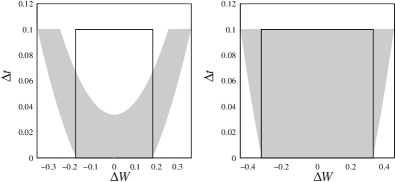
Figure 1: The plots show the regions in $(\Delta t,\Delta W)=(\tau_{n+1}-\tau_{n},W^{j}(\tau_{n+1})-W^{j}(\tau_{n}))$ where $\tau_{n+1}-\tau_{n}\in[0,h]$ and Eq. 5.1 holds (rectangular box) and Eq. 5.3 holds (grey region) hold for $\alpha=1$, $h=0.1$ and (left) $\left\|\mathchoice{\raisebox{0.0pt}{$\displaystyle{\vphantom{\bigm{|}}\mathopen{}q_{jj}(y_{n})}$}}{\smash{q_{jj}(y_{n})}}{q_{jj}(y_{n})}{q_{jj}(y_{n})}\right\|=3$ where $\alpha^{2}<\left\|\mathchoice{\raisebox{0.0pt}{$\displaystyle{\vphantom{\bigm{|}}\mathopen{}q_{jj}(y_{n})}$}}{\smash{q_{jj}(y_{n})}}{q_{jj}(y_{n})}{q_{jj}(y_{n})}\right\|$ and (right) $\left\|\mathchoice{\raisebox{0.0pt}{$\displaystyle{\vphantom{\bigm{|}}\mathopen{}q_{jj}(y_{n})}$}}{\smash{q_{jj}(y_{n})}}{q_{jj}(y_{n})}{q_{jj}(y_{n})}\right\|=0.9$ where $\alpha^{2}>\left\|\mathchoice{\raisebox{0.0pt}{$\displaystyle{\vphantom{\bigm{|}}\mathopen{}q_{jj}(y_{n})}$}}{\smash{q_{jj}(y_{n})}}{q_{jj}(y_{n})}{q_{jj}(y_{n})}\right\|$.

5.1 Pathwise convergence for Adaptive-I

There are two parts to the proof of convergence: first, assuming smoothness of $g_{j}$, we establish that the time steps are not too small in Lemma 5.1 and then, in Theorem 5.2, we show the conditions of Theorem 3.5 hold.

Lemma 5.1.

Suppose that $g_{j}\in\mathrm{C}_{\mathrm{b}}^{2}({}^{d},{}^{d})$ for $j=0,\dots,m$. Choose $(\tau_{0},\dots,\tau_{N})\in{\cal T}$ such that (5.1) holds for parameters $\alpha,h>0$. For all $0<\delta<1$, there exists a random variable $C_{\delta}>0$ (independent of $g_{j}$ and $y_{0}$ and $\alpha$) such that

$$h\leq K_{\operatorname{BI}}|\tau_{n+1}-\tau_{n}|^{1-\delta}\qquad\text{for $n=0,\dots,N-2$,}$$ (5.4)

where $K_{\operatorname{BI}}\coloneq T^{\delta}+{C_{\delta}^{2}\max_{j}\left\|\mathchoice{\raisebox{0.0pt}{$\displaystyle{\vphantom{\bigm{|}}\mathopen{}g_{j}}$}}{\smash{g_{j}}}{g_{j}}{g_{j}}\right\|_{\mathrm{C}_{\mathrm{b}}^{2}}^{2}}/{\alpha^{2}}$.

Proof.

Choose a random variable $C_{\delta}$ such that $|W^{i}(t)-W^{i}(s)|\leq C_{\delta}|t-s|^{(1-\delta)/2}$ for $i=1,\dots,m$ and $0\leq s,t\leq T$.

If $\tau_{n+1}-\tau_{n}=h$, we have $h\leq T^{\delta}|\tau_{n+1}-\tau_{n}|^{1-\delta}$ and Eq. 5.4 holds. Alternatively, $\tau_{n+1}-\tau_{n}<h$ and, as $n\leq N-2$, we know that $\tau_{n+1}<T$. In this case, we must have that $\tau_{n+1}$ satisfies Eq. 5.1 with equality at some specific $i,j=1,\dots,m$. That is,

$$\left\|\mathchoice{\raisebox{0.0pt}{$\displaystyle{\vphantom{\bigm{|}}\mathopen{}q_{ij}(y_{n})}$}}{\smash{q_{ij}(y_{n})}}{q_{ij}(y_{n})}{q_{ij}(y_{n})}\right\|^{1/2}\left|\mathchoice{\raisebox{0.0pt}{$\displaystyle{\vphantom{\bigm{|}}\mathopen{}{W^{i}(\tau_{n+1})-W^{i}(\tau_{n})}}$}}{\smash{{W^{i}(\tau_{n+1})-W^{i}(\tau_{n})}}}{{W^{i}(\tau_{n+1})-W^{i}(\tau_{n})}}{{W^{i}(\tau_{n+1})-W^{i}(\tau_{n})}}\right|=\alpha h^{1/2}.$$

Then,

$$C_{\delta}|\tau_{n+1}-\tau_{n}|^{(1-\delta)/2}\geq\left|\mathchoice{\raisebox{0.0pt}{$\displaystyle{\vphantom{\bigm{|}}\mathopen{}W^{i}(\tau_{n+1})-W^{i}(\tau_{n})}$}}{\smash{W^{i}(\tau_{n+1})-W^{i}(\tau_{n})}}{W^{i}(\tau_{n+1})-W^{i}(\tau_{n})}{W^{i}(\tau_{n+1})-W^{i}(\tau_{n})}\right|=\frac{\alpha h^{1/2}}{\left\|\mathchoice{\raisebox{0.0pt}{$\displaystyle{\vphantom{\bigm{|}}\mathopen{}q_{ij}(y_{n})}$}}{\smash{q_{ij}(y_{n})}}{q_{ij}(y_{n})}{q_{ij}(y_{n})}\right\|^{1/2}}.$$

In other words,

$$h\leq{\frac{C_{\delta}^{2}\left\|\mathchoice{\raisebox{0.0pt}{$\displaystyle{\vphantom{\bigm{|}}\mathopen{}q_{ij}(y_{n})}$}}{\smash{q_{ij}(y_{n})}}{q_{ij}(y_{n})}{q_{ij}(y_{n})}\right\|}{\alpha^{2}}}|\tau_{n+1}-\tau_{n}|^{1-\delta}\leq K_{\operatorname{BI}}|\tau_{n+1}-\tau_{n}|^{1-\delta}$$

for the given $K_{\operatorname{BI}}$, as required. ∎

The next theorem describes an error bound for Adaptive-I. To leading order, the constant $K_{\mathrm{A}}$ in the error bound scales like $\bar{g}^{1+\epsilon}$ for $\bar{g}=\max_{j}\left\|\mathchoice{\raisebox{0.0pt}{$\displaystyle{\vphantom{\bigm{|}}\mathopen{}g_{j}}$}}{\smash{g_{j}}}{g_{j}}{g_{j}}\right\|_{\mathrm{C}_{\mathrm{b}}^{2}}$, whilst the corresponding constant $K_{\mathrm{F}}$ in Theorem 4.2 scales like $\bar{g}^{2}$. This is a more favourable scaling of the error estimate and says the error bound scales nearly linearly with the magnitude of the vector fields $g_{j}$.

Theorem 5.2 (adaptive-I).

Let Assumptions 2.5 and 3.1 hold for the SDE (1.1) and suppose that $g_{j}\in\mathrm{C}_{\mathrm{b}}^{3}({}^{d},{}^{d})$. Let $y_{n}$ denote the Euler–Maruyama approximation (2.1) at times $\tau_{n}$ given by Adaptive-I with $h=T/N$, some $N\in\mathbb{N}$. Then, for $0<\epsilon<1/2$ and $y_{0}\in{}^{d}$, there exists a random variable $K_{\operatorname{A}}>0$ such that, almost surely,

$$\sup_{0\leq\tau_{n}\leq T}\left\|\mathchoice{\raisebox{0.0pt}{$\displaystyle{\vphantom{\bigm{|}}\mathopen{}y_{n}-{y}(\tau_{n};0,{y}_{0})}$}}{\smash{y_{n}-{y}(\tau_{n};0,{y}_{0})}}{y_{n}-{y}(\tau_{n};0,{y}_{0})}{y_{n}-{y}(\tau_{n};0,{y}_{0})}\right\|\leq L_{\operatorname{SDE}}(\epsilon,T)\,K_{\operatorname{A}}\frac{1}{N^{1/2-\epsilon}},\qquad N\geq 1,$$

where $\left\|\mathchoice{\raisebox{0.0pt}{$\displaystyle{\vphantom{\bigm{|}}\mathopen{}K_{\operatorname{A}}}$}}{\smash{K_{\operatorname{A}}}}{K_{\operatorname{A}}}{K_{\operatorname{A}}}\right\|_{L^{p}(\Omega)}\leq K_{1}(\epsilon,p,\alpha,T)\max_{j}\left\|\mathchoice{\raisebox{0.0pt}{$\displaystyle{\vphantom{\bigm{|}}\mathopen{}g_{j}}$}}{\smash{g_{j}}}{g_{j}}{g_{j}}\right\|_{\mathrm{C}_{\mathrm{b}}^{2}}^{1+2\epsilon}+K_{2}(\epsilon,p,\left\|\mathchoice{\raisebox{0.0pt}{$\displaystyle{\vphantom{\bigm{|}}\mathopen{}g_{j}}$}}{\smash{g_{j}}}{g_{j}}{g_{j}}\right\|_{\mathrm{C}_{\mathrm{b}}^{3}},\alpha,T)/N^{1/2}$ for some $K_{1}(\epsilon,p,\alpha,T)$ independent of $g_{j}$ and $N$ and $K_{2}(\epsilon,p,\left\|\mathchoice{\raisebox{0.0pt}{$\displaystyle{\vphantom{\bigm{|}}\mathopen{}g_{j}}$}}{\smash{g_{j}}}{g_{j}}{g_{j}}\right\|_{\mathrm{C}_{\mathrm{b}}^{3}},\alpha,T)$ independent of $N$.

Proof.

We have as in Eq. 4.3

$${X}_{kn}(y_{0})=\sum_{i,j=0}^{m}\int_{t_{k}}^{t_{n}}\int_{{\hat{s\mkern 2.0mu}\mkern-2.0mu}{}}^{s}q_{ij}\left(\mathchoice{\raisebox{0.0pt}{$\displaystyle{\vphantom{\bigm{|}}\mathopen{}y(r;{\hat{r\mkern 2.0mu}\mkern-2.0mu}{},{\hat{y\mkern 1.0mu}\mkern-1.0mu}{}(r))}$}}{y(r;{\hat{r\mkern 2.0mu}\mkern-2.0mu}{},{\hat{y\mkern 1.0mu}\mkern-1.0mu}{}(r))}{y(r;{\hat{r\mkern 2.0mu}\mkern-2.0mu}{},{\hat{y\mkern 1.0mu}\mkern-1.0mu}{}(r))}{y(r;{\hat{r\mkern 2.0mu}\mkern-2.0mu}{},{\hat{y\mkern 1.0mu}\mkern-1.0mu}{}(r))}\right)\,dW^{i}(r)\,dW^{j}(s),\qquad\text{${\hat{y\mkern 1.0mu}\mkern-1.0mu}{}(r)=y_{k}$ if ${\hat{r\mkern 2.0mu}\mkern-2.0mu}{}=\tau_{k}$}.$$

Expanding the terms $i,j=1,\dots,m$ again using Itô’s formula

$$\begin{split}{X}_{kn}(y_{0})&=\sum_{i,j=1}^{m}\int_{t_{k}}^{t_{n}}\int_{{\hat{s\mkern 2.0mu}\mkern-2.0mu}{}}^{s}q_{ij}\left(\mathchoice{\raisebox{0.0pt}{$\displaystyle{\vphantom{\bigm{|}}\mathopen{}y({\hat{r\mkern 2.0mu}\mkern-2.0mu}{};{\hat{r\mkern 2.0mu}\mkern-2.0mu}{},{\hat{y\mkern 1.0mu}\mkern-1.0mu}{}(r))}$}}{y({\hat{r\mkern 2.0mu}\mkern-2.0mu}{};{\hat{r\mkern 2.0mu}\mkern-2.0mu}{},{\hat{y\mkern 1.0mu}\mkern-1.0mu}{}(r))}{y({\hat{r\mkern 2.0mu}\mkern-2.0mu}{};{\hat{r\mkern 2.0mu}\mkern-2.0mu}{},{\hat{y\mkern 1.0mu}\mkern-1.0mu}{}(r))}{y({\hat{r\mkern 2.0mu}\mkern-2.0mu}{};{\hat{r\mkern 2.0mu}\mkern-2.0mu}{},{\hat{y\mkern 1.0mu}\mkern-1.0mu}{}(r))}\right)\,dW^{i}(r)\,dW^{j}(s)\\ &\quad+\sum_{j=0}^{m}\int_{t_{k}}^{t_{n}}\int_{{\hat{s\mkern 2.0mu}\mkern-2.0mu}{}}^{s}q_{0j}\left(\mathchoice{\raisebox{0.0pt}{$\displaystyle{\vphantom{\bigm{|}}\mathopen{}y(r;{\hat{r\mkern 2.0mu}\mkern-2.0mu}{},{\hat{y\mkern 1.0mu}\mkern-1.0mu}{}(r))}$}}{y(r;{\hat{r\mkern 2.0mu}\mkern-2.0mu}{},{\hat{y\mkern 1.0mu}\mkern-1.0mu}{}(r))}{y(r;{\hat{r\mkern 2.0mu}\mkern-2.0mu}{},{\hat{y\mkern 1.0mu}\mkern-1.0mu}{}(r))}{y(r;{\hat{r\mkern 2.0mu}\mkern-2.0mu}{},{\hat{y\mkern 1.0mu}\mkern-1.0mu}{}(r))}\right)\,dr\,dW^{j}(s)\\ &\quad+\sum_{i=1}^{m}\int_{t_{k}}^{t_{n}}\int_{{\hat{s\mkern 2.0mu}\mkern-2.0mu}{}}^{s}q_{i0}\left(\mathchoice{\raisebox{0.0pt}{$\displaystyle{\vphantom{\bigm{|}}\mathopen{}y(r;{\hat{r\mkern 2.0mu}\mkern-2.0mu}{},{\hat{y\mkern 1.0mu}\mkern-1.0mu}{}(r))}$}}{y(r;{\hat{r\mkern 2.0mu}\mkern-2.0mu}{},{\hat{y\mkern 1.0mu}\mkern-1.0mu}{}(r))}{y(r;{\hat{r\mkern 2.0mu}\mkern-2.0mu}{},{\hat{y\mkern 1.0mu}\mkern-1.0mu}{}(r))}{y(r;{\hat{r\mkern 2.0mu}\mkern-2.0mu}{},{\hat{y\mkern 1.0mu}\mkern-1.0mu}{}(r))}\right)\,dW^{i}(r)\,ds\\ &\quad+\sum_{i,j=1,\ell=0}^{m}\int_{t_{k}}^{t_{n}}\int_{{\hat{s\mkern 2.0mu}\mkern-2.0mu}{}}^{s}\int_{{\hat{s\mkern 2.0mu}\mkern-2.0mu}{}}^{r}q_{\ell ij}\left(\mathchoice{\raisebox{0.0pt}{$\displaystyle{\vphantom{\bigm{|}}\mathopen{}y(u;{\hat{u\mkern 2.0mu}\mkern-2.0mu}{},{\hat{y\mkern 1.0mu}\mkern-1.0mu}{}(u))}$}}{y(u;{\hat{u\mkern 2.0mu}\mkern-2.0mu}{},{\hat{y\mkern 1.0mu}\mkern-1.0mu}{}(u))}{y(u;{\hat{u\mkern 2.0mu}\mkern-2.0mu}{},{\hat{y\mkern 1.0mu}\mkern-1.0mu}{}(u))}{y(u;{\hat{u\mkern 2.0mu}\mkern-2.0mu}{},{\hat{y\mkern 1.0mu}\mkern-1.0mu}{}(u))}\right)\,dW^{\ell}(u)\,dW^{i}(r)\,dW^{j}(s),\end{split}$$ (5.5)

where $q_{\ell ij}\coloneq\mathcal{L}^{\ell}q_{ij}$ for $\mathcal{L}^{0}\phi\coloneq D\phi g_{0}+\frac{1}{2}\sum_{j=1}^{m}D^{2}\phi(g_{j},g_{j})$ and $\mathcal{L}^{\ell}\phi\coloneq D\phi g_{\ell}$. Fix $\epsilon\in(0,1/2)$. Following the same arguments as in the proof of Theorem 4.2, the last three terms here are bounded by $K_{\operatorname{TES}}^{2}h^{1-\epsilon}|t_{n}-t_{k}|^{(1+\epsilon)/2}$ for a constant $K_{\operatorname{TES}}^{2}$ that satisfies $\left\|\mathchoice{\raisebox{0.0pt}{$\displaystyle{\vphantom{\bigm{|}}\mathopen{}K_{\operatorname{TES}}^{2}}$}}{\smash{K_{\operatorname{TES}}^{2}}}{K_{\operatorname{TES}}^{2}}{K_{\operatorname{TES}}^{2}}\right\|_{L^{p}(\Omega)}\leq K\left(\mathchoice{\raisebox{0.0pt}{$\displaystyle{\vphantom{\bigm{|}}\mathopen{}\epsilon,\alpha,p,\left\|\mathchoice{\raisebox{0.0pt}{$\displaystyle{\vphantom{\bigm{|}}\mathopen{}g_{j}}$}}{\smash{g_{j}}}{g_{j}}{g_{j}}\right\|_{\mathrm{C}_{\mathrm{b}}^{3}}}$}}{\epsilon,\alpha,p,\left\|\mathchoice{\raisebox{0.0pt}{$\displaystyle{\vphantom{\bigm{|}}\mathopen{}g_{j}}$}}{\smash{g_{j}}}{g_{j}}{g_{j}}\right\|_{\mathrm{C}_{\mathrm{b}}^{3}}}{\epsilon,\alpha,p,\left\|\mathchoice{\raisebox{0.0pt}{$\displaystyle{\vphantom{\bigm{|}}\mathopen{}g_{j}}$}}{\smash{g_{j}}}{g_{j}}{g_{j}}\right\|_{\mathrm{C}_{\mathrm{b}}^{3}}}{\epsilon,\alpha,p,\left\|\mathchoice{\raisebox{0.0pt}{$\displaystyle{\vphantom{\bigm{|}}\mathopen{}g_{j}}$}}{\smash{g_{j}}}{g_{j}}{g_{j}}\right\|_{\mathrm{C}_{\mathrm{b}}^{3}}}\right)$ for some $K\left(\mathchoice{\raisebox{0.0pt}{$\displaystyle{\vphantom{\bigm{|}}\mathopen{}\epsilon,\alpha,p,\left\|\mathchoice{\raisebox{0.0pt}{$\displaystyle{\vphantom{\bigm{|}}\mathopen{}g_{j}}$}}{\smash{g_{j}}}{g_{j}}{g_{j}}\right\|_{\mathrm{C}_{\mathrm{b}}^{3}}}$}}{\epsilon,\alpha,p,\left\|\mathchoice{\raisebox{0.0pt}{$\displaystyle{\vphantom{\bigm{|}}\mathopen{}g_{j}}$}}{\smash{g_{j}}}{g_{j}}{g_{j}}\right\|_{\mathrm{C}_{\mathrm{b}}^{3}}}{\epsilon,\alpha,p,\left\|\mathchoice{\raisebox{0.0pt}{$\displaystyle{\vphantom{\bigm{|}}\mathopen{}g_{j}}$}}{\smash{g_{j}}}{g_{j}}{g_{j}}\right\|_{\mathrm{C}_{\mathrm{b}}^{3}}}{\epsilon,\alpha,p,\left\|\mathchoice{\raisebox{0.0pt}{$\displaystyle{\vphantom{\bigm{|}}\mathopen{}g_{j}}$}}{\smash{g_{j}}}{g_{j}}{g_{j}}\right\|_{\mathrm{C}_{\mathrm{b}}^{3}}}\right)$ independent of $N$.

To bound the first term, we use a more refined argument. Let $\bar{g}\coloneq\max_{j}\left\|\mathchoice{\raisebox{0.0pt}{$\displaystyle{\vphantom{\bigm{|}}\mathopen{}g_{j}}$}}{\smash{g_{j}}}{g_{j}}{g_{j}}\right\|_{\mathrm{C}_{\mathrm{b}}^{2}}$ and

$$\phi_{N}(s)\coloneq\frac{1}{\bar{g}h^{1/2}}\int_{{\hat{s\mkern 2.0mu}\mkern-2.0mu}{}}^{s}q_{ij}\left(\mathchoice{\raisebox{0.0pt}{$\displaystyle{\vphantom{\bigm{|}}\mathopen{}y({\hat{r\mkern 2.0mu}\mkern-2.0mu}{};{\hat{r\mkern 2.0mu}\mkern-2.0mu}{},{\hat{y\mkern 1.0mu}\mkern-1.0mu}{}(r))}$}}{y({\hat{r\mkern 2.0mu}\mkern-2.0mu}{};{\hat{r\mkern 2.0mu}\mkern-2.0mu}{},{\hat{y\mkern 1.0mu}\mkern-1.0mu}{}(r))}{y({\hat{r\mkern 2.0mu}\mkern-2.0mu}{};{\hat{r\mkern 2.0mu}\mkern-2.0mu}{},{\hat{y\mkern 1.0mu}\mkern-1.0mu}{}(r))}{y({\hat{r\mkern 2.0mu}\mkern-2.0mu}{};{\hat{r\mkern 2.0mu}\mkern-2.0mu}{},{\hat{y\mkern 1.0mu}\mkern-1.0mu}{}(r))}\right)\,dW^{i}(r)=\frac{1}{\bar{g}h^{1/2}}\int_{{\hat{s\mkern 2.0mu}\mkern-2.0mu}{}}^{s}q_{ij}\left(\mathchoice{\raisebox{0.0pt}{$\displaystyle{\vphantom{\bigm{|}}\mathopen{}{\hat{y\mkern 1.0mu}\mkern-1.0mu}{}(r)}$}}{{\hat{y\mkern 1.0mu}\mkern-1.0mu}{}(r)}{{\hat{y\mkern 1.0mu}\mkern-1.0mu}{}(r)}{{\hat{y\mkern 1.0mu}\mkern-1.0mu}{}(r)}\right)\,dW^{i}(r)$$

for $\tau_{k}={\hat{r\mkern 2.0mu}\mkern-2.0mu}{}\leq r<\tau_{k+1}$. Here $\phi_{N}(s)$ is continuous and adapted (as ${\hat{s\mkern 2.0mu}\mkern-2.0mu}{}$ is a stopping time and ${\hat{s\mkern 2.0mu}\mkern-2.0mu}{}<s$) and hence predictable. By Eq. 5.1,

$$\left\|\mathchoice{\raisebox{0.0pt}{$\displaystyle{\vphantom{\bigm{|}}\mathopen{}q_{ij}\left(\mathchoice{\raisebox{0.0pt}{$\displaystyle{\vphantom{\bigm{|}}\mathopen{}y({\hat{r\mkern 2.0mu}\mkern-2.0mu}{};{\hat{r\mkern 2.0mu}\mkern-2.0mu}{},{\hat{y\mkern 1.0mu}\mkern-1.0mu}{}(r))}$}}{y({\hat{r\mkern 2.0mu}\mkern-2.0mu}{};{\hat{r\mkern 2.0mu}\mkern-2.0mu}{},{\hat{y\mkern 1.0mu}\mkern-1.0mu}{}(r))}{y({\hat{r\mkern 2.0mu}\mkern-2.0mu}{};{\hat{r\mkern 2.0mu}\mkern-2.0mu}{},{\hat{y\mkern 1.0mu}\mkern-1.0mu}{}(r))}{y({\hat{r\mkern 2.0mu}\mkern-2.0mu}{};{\hat{r\mkern 2.0mu}\mkern-2.0mu}{},{\hat{y\mkern 1.0mu}\mkern-1.0mu}{}(r))}\right)}$}}{\smash{q_{ij}\left(\mathchoice{\raisebox{0.0pt}{$\displaystyle{\vphantom{\bigm{|}}\mathopen{}y({\hat{r\mkern 2.0mu}\mkern-2.0mu}{};{\hat{r\mkern 2.0mu}\mkern-2.0mu}{},{\hat{y\mkern 1.0mu}\mkern-1.0mu}{}(r))}$}}{y({\hat{r\mkern 2.0mu}\mkern-2.0mu}{};{\hat{r\mkern 2.0mu}\mkern-2.0mu}{},{\hat{y\mkern 1.0mu}\mkern-1.0mu}{}(r))}{y({\hat{r\mkern 2.0mu}\mkern-2.0mu}{};{\hat{r\mkern 2.0mu}\mkern-2.0mu}{},{\hat{y\mkern 1.0mu}\mkern-1.0mu}{}(r))}{y({\hat{r\mkern 2.0mu}\mkern-2.0mu}{};{\hat{r\mkern 2.0mu}\mkern-2.0mu}{},{\hat{y\mkern 1.0mu}\mkern-1.0mu}{}(r))}\right)}}{q_{ij}\left(\mathchoice{\raisebox{0.0pt}{$\displaystyle{\vphantom{\bigm{|}}\mathopen{}y({\hat{r\mkern 2.0mu}\mkern-2.0mu}{};{\hat{r\mkern 2.0mu}\mkern-2.0mu}{},{\hat{y\mkern 1.0mu}\mkern-1.0mu}{}(r))}$}}{y({\hat{r\mkern 2.0mu}\mkern-2.0mu}{};{\hat{r\mkern 2.0mu}\mkern-2.0mu}{},{\hat{y\mkern 1.0mu}\mkern-1.0mu}{}(r))}{y({\hat{r\mkern 2.0mu}\mkern-2.0mu}{};{\hat{r\mkern 2.0mu}\mkern-2.0mu}{},{\hat{y\mkern 1.0mu}\mkern-1.0mu}{}(r))}{y({\hat{r\mkern 2.0mu}\mkern-2.0mu}{};{\hat{r\mkern 2.0mu}\mkern-2.0mu}{},{\hat{y\mkern 1.0mu}\mkern-1.0mu}{}(r))}\right)}{q_{ij}\left(\mathchoice{\raisebox{0.0pt}{$\displaystyle{\vphantom{\bigm{|}}\mathopen{}y({\hat{r\mkern 2.0mu}\mkern-2.0mu}{};{\hat{r\mkern 2.0mu}\mkern-2.0mu}{},{\hat{y\mkern 1.0mu}\mkern-1.0mu}{}(r))}$}}{y({\hat{r\mkern 2.0mu}\mkern-2.0mu}{};{\hat{r\mkern 2.0mu}\mkern-2.0mu}{},{\hat{y\mkern 1.0mu}\mkern-1.0mu}{}(r))}{y({\hat{r\mkern 2.0mu}\mkern-2.0mu}{};{\hat{r\mkern 2.0mu}\mkern-2.0mu}{},{\hat{y\mkern 1.0mu}\mkern-1.0mu}{}(r))}{y({\hat{r\mkern 2.0mu}\mkern-2.0mu}{};{\hat{r\mkern 2.0mu}\mkern-2.0mu}{},{\hat{y\mkern 1.0mu}\mkern-1.0mu}{}(r))}\right)}\right\|^{1/2}\,\left|\mathchoice{\raisebox{0.0pt}{$\displaystyle{\vphantom{\bigm{|}}\mathopen{}W^{i}(\tau_{n+1})-W^{i}(\tau_{n})}$}}{\smash{W^{i}(\tau_{n+1})-W^{i}(\tau_{n})}}{W^{i}(\tau_{n+1})-W^{i}(\tau_{n})}{W^{i}(\tau_{n+1})-W^{i}(\tau_{n})}\right|\leq\alpha h^{1/2},\qquad j=1,\dots,m.$$

As $\left\|\mathchoice{\raisebox{0.0pt}{$\displaystyle{\vphantom{\bigm{|}}\mathopen{}q_{ij}}$}}{\smash{q_{ij}}}{q_{ij}}{q_{ij}}\right\|\leq\bar{g}^{2}$, this gives

$$\sup_{0\leq s\leq T}\left\|\mathchoice{\raisebox{0.0pt}{$\displaystyle{\vphantom{\bigm{|}}\mathopen{}\phi_{N}(s)}$}}{\smash{\phi_{N}(s)}}{\phi_{N}(s)}{\phi_{N}(s)}\right\|^{2}=\frac{1}{\bar{g}^{2}h}\sup_{0\leq s\leq T}\left\|\mathchoice{\raisebox{0.0pt}{$\displaystyle{\vphantom{\bigm{|}}\mathopen{}\int_{{\hat{s\mkern 2.0mu}\mkern-2.0mu}{}}^{s}{q_{ij}\left(\mathchoice{\raisebox{0.0pt}{$\displaystyle{\vphantom{\bigm{|}}\mathopen{}y({\hat{r\mkern 2.0mu}\mkern-2.0mu}{};{\hat{r\mkern 2.0mu}\mkern-2.0mu}{},{\hat{y\mkern 1.0mu}\mkern-1.0mu}{}(r))}$}}{y({\hat{r\mkern 2.0mu}\mkern-2.0mu}{};{\hat{r\mkern 2.0mu}\mkern-2.0mu}{},{\hat{y\mkern 1.0mu}\mkern-1.0mu}{}(r))}{y({\hat{r\mkern 2.0mu}\mkern-2.0mu}{};{\hat{r\mkern 2.0mu}\mkern-2.0mu}{},{\hat{y\mkern 1.0mu}\mkern-1.0mu}{}(r))}{y({\hat{r\mkern 2.0mu}\mkern-2.0mu}{};{\hat{r\mkern 2.0mu}\mkern-2.0mu}{},{\hat{y\mkern 1.0mu}\mkern-1.0mu}{}(r))}\right)}\,dW^{i}(r)}$}}{\smash{\int_{{\hat{s\mkern 2.0mu}\mkern-2.0mu}{}}^{s}{q_{ij}\left(\mathchoice{\raisebox{0.0pt}{$\displaystyle{\vphantom{\bigm{|}}\mathopen{}y({\hat{r\mkern 2.0mu}\mkern-2.0mu}{};{\hat{r\mkern 2.0mu}\mkern-2.0mu}{},{\hat{y\mkern 1.0mu}\mkern-1.0mu}{}(r))}$}}{y({\hat{r\mkern 2.0mu}\mkern-2.0mu}{};{\hat{r\mkern 2.0mu}\mkern-2.0mu}{},{\hat{y\mkern 1.0mu}\mkern-1.0mu}{}(r))}{y({\hat{r\mkern 2.0mu}\mkern-2.0mu}{};{\hat{r\mkern 2.0mu}\mkern-2.0mu}{},{\hat{y\mkern 1.0mu}\mkern-1.0mu}{}(r))}{y({\hat{r\mkern 2.0mu}\mkern-2.0mu}{};{\hat{r\mkern 2.0mu}\mkern-2.0mu}{},{\hat{y\mkern 1.0mu}\mkern-1.0mu}{}(r))}\right)}\,dW^{i}(r)}}{\int_{{\hat{s\mkern 2.0mu}\mkern-2.0mu}{}}^{s}{q_{ij}\left(\mathchoice{\raisebox{0.0pt}{$\displaystyle{\vphantom{\bigm{|}}\mathopen{}y({\hat{r\mkern 2.0mu}\mkern-2.0mu}{};{\hat{r\mkern 2.0mu}\mkern-2.0mu}{},{\hat{y\mkern 1.0mu}\mkern-1.0mu}{}(r))}$}}{y({\hat{r\mkern 2.0mu}\mkern-2.0mu}{};{\hat{r\mkern 2.0mu}\mkern-2.0mu}{},{\hat{y\mkern 1.0mu}\mkern-1.0mu}{}(r))}{y({\hat{r\mkern 2.0mu}\mkern-2.0mu}{};{\hat{r\mkern 2.0mu}\mkern-2.0mu}{},{\hat{y\mkern 1.0mu}\mkern-1.0mu}{}(r))}{y({\hat{r\mkern 2.0mu}\mkern-2.0mu}{};{\hat{r\mkern 2.0mu}\mkern-2.0mu}{},{\hat{y\mkern 1.0mu}\mkern-1.0mu}{}(r))}\right)}\,dW^{i}(r)}{\int_{{\hat{s\mkern 2.0mu}\mkern-2.0mu}{}}^{s}{q_{ij}\left(\mathchoice{\raisebox{0.0pt}{$\displaystyle{\vphantom{\bigm{|}}\mathopen{}y({\hat{r\mkern 2.0mu}\mkern-2.0mu}{};{\hat{r\mkern 2.0mu}\mkern-2.0mu}{},{\hat{y\mkern 1.0mu}\mkern-1.0mu}{}(r))}$}}{y({\hat{r\mkern 2.0mu}\mkern-2.0mu}{};{\hat{r\mkern 2.0mu}\mkern-2.0mu}{},{\hat{y\mkern 1.0mu}\mkern-1.0mu}{}(r))}{y({\hat{r\mkern 2.0mu}\mkern-2.0mu}{};{\hat{r\mkern 2.0mu}\mkern-2.0mu}{},{\hat{y\mkern 1.0mu}\mkern-1.0mu}{}(r))}{y({\hat{r\mkern 2.0mu}\mkern-2.0mu}{};{\hat{r\mkern 2.0mu}\mkern-2.0mu}{},{\hat{y\mkern 1.0mu}\mkern-1.0mu}{}(r))}\right)}\,dW^{i}(r)}\right\|^{2}\leq\alpha^{2}.$$

Hence, Eq. 4.1 holds and Lemma 4.1 applies with $\lambda=1/2$ and

$$X^{N}(t)=h^{1/2}\int_{0}^{t}\phi_{N}(s)\,dW^{i}(s).$$

This gives a $c_{ij}\in L^{p}(\Omega)$ such that

$$\frac{1}{\bar{g}}\left\|\mathchoice{\raisebox{0.0pt}{$\displaystyle{\vphantom{\bigm{|}}\mathopen{}\int_{\tau_{k}}^{\tau_{n}}\int_{{\hat{s\mkern 2.0mu}\mkern-2.0mu}{}}^{s}q_{ij}\left(\mathchoice{\raisebox{0.0pt}{$\displaystyle{\vphantom{\bigm{|}}\mathopen{}y({\hat{r\mkern 2.0mu}\mkern-2.0mu}{};{\hat{r\mkern 2.0mu}\mkern-2.0mu}{},{\hat{y\mkern 1.0mu}\mkern-1.0mu}{}(r))}$}}{y({\hat{r\mkern 2.0mu}\mkern-2.0mu}{};{\hat{r\mkern 2.0mu}\mkern-2.0mu}{},{\hat{y\mkern 1.0mu}\mkern-1.0mu}{}(r))}{y({\hat{r\mkern 2.0mu}\mkern-2.0mu}{};{\hat{r\mkern 2.0mu}\mkern-2.0mu}{},{\hat{y\mkern 1.0mu}\mkern-1.0mu}{}(r))}{y({\hat{r\mkern 2.0mu}\mkern-2.0mu}{};{\hat{r\mkern 2.0mu}\mkern-2.0mu}{},{\hat{y\mkern 1.0mu}\mkern-1.0mu}{}(r))}\right)\,dW^{i}(r)\,dW^{j}(s)}$}}{\smash{\int_{\tau_{k}}^{\tau_{n}}\int_{{\hat{s\mkern 2.0mu}\mkern-2.0mu}{}}^{s}q_{ij}\left(\mathchoice{\raisebox{0.0pt}{$\displaystyle{\vphantom{\bigm{|}}\mathopen{}y({\hat{r\mkern 2.0mu}\mkern-2.0mu}{};{\hat{r\mkern 2.0mu}\mkern-2.0mu}{},{\hat{y\mkern 1.0mu}\mkern-1.0mu}{}(r))}$}}{y({\hat{r\mkern 2.0mu}\mkern-2.0mu}{};{\hat{r\mkern 2.0mu}\mkern-2.0mu}{},{\hat{y\mkern 1.0mu}\mkern-1.0mu}{}(r))}{y({\hat{r\mkern 2.0mu}\mkern-2.0mu}{};{\hat{r\mkern 2.0mu}\mkern-2.0mu}{},{\hat{y\mkern 1.0mu}\mkern-1.0mu}{}(r))}{y({\hat{r\mkern 2.0mu}\mkern-2.0mu}{};{\hat{r\mkern 2.0mu}\mkern-2.0mu}{},{\hat{y\mkern 1.0mu}\mkern-1.0mu}{}(r))}\right)\,dW^{i}(r)\,dW^{j}(s)}}{\int_{\tau_{k}}^{\tau_{n}}\int_{{\hat{s\mkern 2.0mu}\mkern-2.0mu}{}}^{s}q_{ij}\left(\mathchoice{\raisebox{0.0pt}{$\displaystyle{\vphantom{\bigm{|}}\mathopen{}y({\hat{r\mkern 2.0mu}\mkern-2.0mu}{};{\hat{r\mkern 2.0mu}\mkern-2.0mu}{},{\hat{y\mkern 1.0mu}\mkern-1.0mu}{}(r))}$}}{y({\hat{r\mkern 2.0mu}\mkern-2.0mu}{};{\hat{r\mkern 2.0mu}\mkern-2.0mu}{},{\hat{y\mkern 1.0mu}\mkern-1.0mu}{}(r))}{y({\hat{r\mkern 2.0mu}\mkern-2.0mu}{};{\hat{r\mkern 2.0mu}\mkern-2.0mu}{},{\hat{y\mkern 1.0mu}\mkern-1.0mu}{}(r))}{y({\hat{r\mkern 2.0mu}\mkern-2.0mu}{};{\hat{r\mkern 2.0mu}\mkern-2.0mu}{},{\hat{y\mkern 1.0mu}\mkern-1.0mu}{}(r))}\right)\,dW^{i}(r)\,dW^{j}(s)}{\int_{\tau_{k}}^{\tau_{n}}\int_{{\hat{s\mkern 2.0mu}\mkern-2.0mu}{}}^{s}q_{ij}\left(\mathchoice{\raisebox{0.0pt}{$\displaystyle{\vphantom{\bigm{|}}\mathopen{}y({\hat{r\mkern 2.0mu}\mkern-2.0mu}{};{\hat{r\mkern 2.0mu}\mkern-2.0mu}{},{\hat{y\mkern 1.0mu}\mkern-1.0mu}{}(r))}$}}{y({\hat{r\mkern 2.0mu}\mkern-2.0mu}{};{\hat{r\mkern 2.0mu}\mkern-2.0mu}{},{\hat{y\mkern 1.0mu}\mkern-1.0mu}{}(r))}{y({\hat{r\mkern 2.0mu}\mkern-2.0mu}{};{\hat{r\mkern 2.0mu}\mkern-2.0mu}{},{\hat{y\mkern 1.0mu}\mkern-1.0mu}{}(r))}{y({\hat{r\mkern 2.0mu}\mkern-2.0mu}{};{\hat{r\mkern 2.0mu}\mkern-2.0mu}{},{\hat{y\mkern 1.0mu}\mkern-1.0mu}{}(r))}\right)\,dW^{i}(r)\,dW^{j}(s)}\right\|\leq c_{ij}\,{|\tau_{n}-\tau_{k}|^{1/2-\epsilon/4}}\,{h^{1/2-\epsilon/8}}.$$

We may choose $c_{ij}$ so that its $L^{p}(\Omega)$ norm is independent of $h$ and $\bar{g}$. This provides the necessary bound on the first term of Eq. 5.5.

Taken all the terms in Eq. 5.5 together, we can find $K_{\operatorname{TES}}^{1}$ such that

$$X_{kn}(y_{0})\leq K_{\operatorname{TES}}^{1}{|\tau_{n}-\tau_{k}|^{1/2-\epsilon/4}}{h^{1/2-\epsilon/8}}+K_{\operatorname{TES}}^{2}{}{h^{1-\epsilon}}|\tau_{n}-\tau_{k}|^{(1+\epsilon)/2}.$$

Here $\left\|\mathchoice{\raisebox{0.0pt}{$\displaystyle{\vphantom{\bigm{|}}\mathopen{}K_{\operatorname{TES}}^{1}}$}}{\smash{K_{\operatorname{TES}}^{1}}}{K_{\operatorname{TES}}^{1}}{K_{\operatorname{TES}}^{1}}\right\|_{L^{p}(\Omega)}\leq\bar{g}K(\epsilon,p,\alpha,T)$ for some $K(\epsilon,p,\alpha,T)$ independent of $N$ and $g_{j}$.

Using Lemma 5.1 with $\delta=1/7$, we have the lower bound $h\leq K_{\operatorname{BI}}|\tau_{n}-\tau_{k}|^{1-\delta}=K_{\operatorname{BI}}\left|\mathchoice{\raisebox{0.0pt}{$\displaystyle{\vphantom{\bigm{|}}\mathopen{}\tau_{n}-\tau_{k}}$}}{\smash{\tau_{n}-\tau_{k}}}{\tau_{n}-\tau_{k}}{\tau_{n}-\tau_{k}}\right|^{6/7}$ on the time step for $k,n=0,\dots,N-1$. Hence,

$$|\tau_{n}-\tau_{k}|^{1/2-\epsilon/4}h^{1/2-\epsilon/8} \leq|\tau_{n}-\tau_{k}|^{1/2-\epsilon/4}{h^{1/2-\epsilon}}{h^{7\epsilon/8}}$$

$$\leq|\tau_{n}-\tau_{k}|^{1/2-\epsilon/4}{h^{1/2-\epsilon}}\,K_{\operatorname{BI}}^{7\epsilon/8}\,|\tau_{n}-\tau_{k}|^{\epsilon 3/4}$$

$$=|\tau_{n}-\tau_{k}|^{1/2+\epsilon/2}\,{h^{1/2-\epsilon}}K_{\operatorname{BI}}^{7\epsilon/8}.$$

Consequently,

$$\left\|\mathchoice{\raisebox{0.0pt}{$\displaystyle{\vphantom{\bigm{|}}\mathopen{}X_{kn}(y_{0})}$}}{\smash{X_{kn}(y_{0})}}{X_{kn}(y_{0})}{X_{kn}(y_{0})}\right\|\leq K_{\operatorname{TES}}^{1}K_{\operatorname{BI}}^{\epsilon}{|\tau_{n}-\tau_{k}|^{(1+\epsilon)/2}}{h^{1/2-\epsilon}}+K_{\operatorname{TES}}^{2}|\tau_{n}-\tau_{k}|^{(1+\epsilon)/2}h^{1-\epsilon}.$$

We have all the conditions of Theorem 3.5, which gives the desired error bound for $n=0,\dots,N-1$. The final step from $\tau_{N-1}$ to $\tau_{N}$ may equal $|T-\tau_{N-1}|$, which may be very small and does not yield to Lemma 5.1. However, the error resulting from this step can be added into the $K_{\operatorname{TES}}^{2}$ term by utilising the bound in Eq. 2.6. ∎

5.2 Analysis of Adaptive-II

The convergence result (Theorem 5.4 below) for Euler–Maruyama with Adaptive-II is similar to Theorem 5.2 and the new time-stepping strategy behaves like Adaptive-I. However, the method of proof is different and we will make use of Azuma’s inequality. First, we show the time step does not become too small, similarly to Lemma 5.1.

Lemma 5.3.

Suppose that $g_{j}\in\mathrm{C}_{\mathrm{b}}^{2}({}^{d},{}^{d})$ for $j=0,\dots,m$. Choose $(\tau_{0},\dots,\tau_{N})\in\mathcal{T}$ such that Eq. 5.2 holds for parameters $\alpha,h>0$. For $0<\delta<1$, there exists a random variable $C_{\delta}>0$ (independent of $\alpha$, $h$, $g_{j}$, and $y_{0}$) such that

$$h\leq K_{\operatorname{BI}}|\tau_{k+1}-\tau_{k}|^{1-\delta},\quad\text{for $k=0,\dots,N-2$,}$$ (5.6)

where $K_{\operatorname{BI}}=T^{\delta}+{{2C_{\delta}\max_{j}\left\|\mathchoice{\raisebox{0.0pt}{$\displaystyle{\vphantom{\bigm{|}}\mathopen{}g_{j}}$}}{\smash{g_{j}}}{g_{j}}{g_{j}}\right\|_{\mathrm{C}_{\mathrm{b}}^{2}}^{2}/\alpha^{2}}}$.

Proof.

Choose a random variable $C_{\delta}$ such that $\left|\mathchoice{\raisebox{0.0pt}{$\displaystyle{\vphantom{\bigm{|}}\mathopen{}\int_{s}^{t}W^{i}(r)\,dW^{j}(r)}$}}{\smash{\int_{s}^{t}W^{i}(r)\,dW^{j}(r)}}{\int_{s}^{t}W^{i}(r)\,dW^{j}(r)}{\int_{s}^{t}W^{i}(r)\,dW^{j}(r)}\right|\leq C_{\delta}|t-s|^{1-\delta}$ for $i,j=1,\dots,m$ and $0\leq s,t\leq T$.

If $\tau_{k+1}-\tau_{k}=h$, then $h\leq T^{\delta}|\tau_{k+1}-\tau_{k}|^{1-\delta}$ and Eq. 5.6 holds. Otherwise, we must have $\tau_{k+1}-\tau_{k}<h$ and $\tau_{k+1}<T$. Then $\tau_{k+1}$ satisfies Eq. 5.2 with equality for some $i,j=1,\dots,m$:

$$\left\|\mathchoice{\raisebox{0.0pt}{$\displaystyle{\vphantom{\bigm{|}}\mathopen{}q_{ij}(y_{k})}$}}{\smash{q_{ij}(y_{k})}}{q_{ij}(y_{k})}{q_{ij}(y_{k})}\right\|\,\left|\mathchoice{\raisebox{0.0pt}{$\displaystyle{\vphantom{\bigm{|}}\mathopen{}\int_{\tau_{k}}^{\tau_{k+1}}\int_{\tau_{k}}^{s}\,dW^{i}(r)\,dW^{j}(s)}$}}{\smash{\int_{\tau_{k}}^{\tau_{k+1}}\int_{\tau_{k}}^{s}\,dW^{i}(r)\,dW^{j}(s)}}{\int_{\tau_{k}}^{\tau_{k+1}}\int_{\tau_{k}}^{s}\,dW^{i}(r)\,dW^{j}(s)}{\int_{\tau_{k}}^{\tau_{k+1}}\int_{\tau_{k}}^{s}\,dW^{i}(r)\,dW^{j}(s)}\right|=\frac{1}{2}\alpha^{2}h.$$

Then,

$$C_{\delta}|\tau_{k+1}-\tau_{k}|^{1-\delta}\geq\left|\mathchoice{\raisebox{0.0pt}{$\displaystyle{\vphantom{\bigm{|}}\mathopen{}\int_{\tau_{k}}^{\tau_{k+1}}\int_{\tau_{k}}^{s}\,W^{i}(r)\,dW^{j}(s)}$}}{\smash{\int_{\tau_{k}}^{\tau_{k+1}}\int_{\tau_{k}}^{s}\,W^{i}(r)\,dW^{j}(s)}}{\int_{\tau_{k}}^{\tau_{k+1}}\int_{\tau_{k}}^{s}\,W^{i}(r)\,dW^{j}(s)}{\int_{\tau_{k}}^{\tau_{k+1}}\int_{\tau_{k}}^{s}\,W^{i}(r)\,dW^{j}(s)}\right|\geq\frac{\alpha^{2}h}{2\left\|\mathchoice{\raisebox{0.0pt}{$\displaystyle{\vphantom{\bigm{|}}\mathopen{}q_{ij}(y_{k})}$}}{\smash{q_{ij}(y_{k})}}{q_{ij}(y_{k})}{q_{ij}(y_{k})}\right\|}.$$

In other words,

$$h\leq{\frac{2C_{\delta}\left\|\mathchoice{\raisebox{0.0pt}{$\displaystyle{\vphantom{\bigm{|}}\mathopen{}q_{ij}(y_{k})}$}}{\smash{q_{ij}(y_{k})}}{q_{ij}(y_{k})}{q_{ij}(y_{k})}\right\|}{\alpha^{2}}}|\tau_{k+1}-\tau_{k}|^{1-\delta}\leq K_{\operatorname{BI}}|\tau_{k+1}-\tau_{k}|^{1-\delta}.$$

Thus, Eq. 5.6 holds and the proof is complete. ∎

The error bound for Adaptive-II found in the next theorem scales (in terms of $g_{j}$) like the one for Adaptive-I.

Theorem 5.4 (adaptive-II).

Let Assumptions 2.5 and 3.1 hold for the SDE (1.1) and suppose that $g_{j}\in\mathrm{C}_{\mathrm{b}}^{3}({}^{d},{}^{d})$. Let $y_{n}$ denote the Euler–Maruyama approximation at times $\tau_{n}$ with adaptive increments given by Eqs. 5.2 and 2.1. Then, for $0<\epsilon<1/2$ and $y_{0}\in{}^{d}$, there exists a random variable $K_{\operatorname{A}}>0$ such that, almost surely,

$$\sup_{0\leq\tau_{n}\leq T}\left\|\mathchoice{\raisebox{0.0pt}{$\displaystyle{\vphantom{\bigm{|}}\mathopen{}y_{n}-{y}(\tau_{n};0,{y}_{0})}$}}{\smash{y_{n}-{y}(\tau_{n};0,{y}_{0})}}{y_{n}-{y}(\tau_{n};0,{y}_{0})}{y_{n}-{y}(\tau_{n};0,{y}_{0})}\right\|\leq L_{\operatorname{SDE}}(\epsilon,T)\,K_{\operatorname{A}}\frac{1}{N^{1/2-\epsilon}},\qquad N\geq 1,$$

where $\left\|\mathchoice{\raisebox{0.0pt}{$\displaystyle{\vphantom{\bigm{|}}\mathopen{}K_{\operatorname{A}}}$}}{\smash{K_{\operatorname{A}}}}{K_{\operatorname{A}}}{K_{\operatorname{A}}}\right\|_{L^{p}(\Omega)}\leq K_{1}(\epsilon,p,\alpha,T)\left\|\mathchoice{\raisebox{0.0pt}{$\displaystyle{\vphantom{\bigm{|}}\mathopen{}g_{j}}$}}{\smash{g_{j}}}{g_{j}}{g_{j}}\right\|_{\mathrm{C}_{\mathrm{b}}^{2}}^{1+\epsilon}+K_{2}(\epsilon,p,\alpha,\left\|\mathchoice{\raisebox{0.0pt}{$\displaystyle{\vphantom{\bigm{|}}\mathopen{}g_{j}}$}}{\smash{g_{j}}}{g_{j}}{g_{j}}\right\|_{\mathrm{C}_{\mathrm{b}}^{3}},T)/N^{1/2}$ for some $K_{1}(\epsilon,p,\alpha,T)$ independent of $N$ and $g_{j}$, and some $K_{2}(\epsilon,p,\alpha,\left\|\mathchoice{\raisebox{0.0pt}{$\displaystyle{\vphantom{\bigm{|}}\mathopen{}g_{j}}$}}{\smash{g_{j}}}{g_{j}}{g_{j}}\right\|_{\mathrm{C}_{\mathrm{b}}^{3}},T)$ independent of $N$.

Proof.

Following the proof of Theorem 5.2, it is enough to treat the term

$$S_{kn}\coloneq\sum_{j=k}^{n-1}S_{j},\qquad\text{for }S_{k}\coloneq\sum_{i,j=1}^{m}\int_{\tau_{k}}^{\tau_{k+1}}\int_{\tau_{k}}^{s}q_{ij}(y_{k})\,dW^{i}(r)\,dW^{j}(s)\text{ and $0\leq k<n\leq N$,}$$

and show it satisfies the condition on $X_{kn}$ in Assumption 3.2. By the optional stopping theorem, each $S_{k}$ has mean zero and, by Eq. 5.2, $\left\|\mathchoice{\raisebox{0.0pt}{$\displaystyle{\vphantom{\bigm{|}}\mathopen{}S_{k}}$}}{\smash{S_{k}}}{S_{k}}{S_{k}}\right\|\leq m^{2}\alpha^{2}h/2$ for $h=T/N$. Then, $S_{kn}$ is a sum independent random variables, each with mean zero and bounded by $m^{2}\alpha^{2}h/2$ . Azuma’s inequality (see Lemma A.3 with $\lambda=(n-k)^{1/2}h^{1-\epsilon/4}$) gives

$$\mathbb{P}\left(\mathchoice{\raisebox{0.0pt}{$\displaystyle{\vphantom{\bigm{|}}\mathopen{}\left\|\mathchoice{\raisebox{0.0pt}{$\displaystyle{\vphantom{\bigm{|}}\mathopen{}S_{kn}}$}}{\smash{S_{kn}}}{S_{kn}}{S_{kn}}\right\|\geq\lambda}$}}{\left\|\mathchoice{\raisebox{0.0pt}{$\displaystyle{\vphantom{\bigm{|}}\mathopen{}S_{kn}}$}}{\smash{S_{kn}}}{S_{kn}}{S_{kn}}\right\|\geq\lambda}{\left\|\mathchoice{\raisebox{0.0pt}{$\displaystyle{\vphantom{\bigm{|}}\mathopen{}S_{kn}}$}}{\smash{S_{kn}}}{S_{kn}}{S_{kn}}\right\|\geq\lambda}{\left\|\mathchoice{\raisebox{0.0pt}{$\displaystyle{\vphantom{\bigm{|}}\mathopen{}S_{kn}}$}}{\smash{S_{kn}}}{S_{kn}}{S_{kn}}\right\|\geq\lambda}\right)\leq 2\exp\left(\mathchoice{\raisebox{0.0pt}{$\displaystyle{\vphantom{\bigm{|}}\mathopen{}\frac{-4\lambda^{2}}{2(n-k)m^{4}\alpha^{4}h^{2}}}$}}{\frac{-4\lambda^{2}}{2(n-k)m^{4}\alpha^{4}h^{2}}}{\frac{-4\lambda^{2}}{2(n-k)m^{4}\alpha^{4}h^{2}}}{\frac{-4\lambda^{2}}{2(n-k)m^{4}\alpha^{4}h^{2}}}\right)=2\exp\left(\mathchoice{\raisebox{0.0pt}{$\displaystyle{\vphantom{\bigm{|}}\mathopen{}\frac{-2}{m^{4}\alpha^{4}h^{\epsilon/2}}}$}}{\frac{-2}{m^{4}\alpha^{4}h^{\epsilon/2}}}{\frac{-2}{m^{4}\alpha^{4}h^{\epsilon/2}}}{\frac{-2}{m^{4}\alpha^{4}h^{\epsilon/2}}}\right).$$

Let $F_{N}\coloneq\{\omega\in\Omega\colon\sup_{0\leq k<n\leq N}\left\|\mathchoice{\raisebox{0.0pt}{$\displaystyle{\vphantom{\bigm{|}}\mathopen{}S_{kn}(\omega)}$}}{\smash{S_{kn}(\omega)}}{S_{kn}(\omega)}{S_{kn}(\omega)}\right\|/(n-k)^{1/2}\geq h^{1-\epsilon/4}\}$. Using $h=T/N$,

$$\mathbb{P}\left(\mathchoice{\raisebox{0.0pt}{$\displaystyle{\vphantom{\bigm{|}}\mathopen{}F_{N}}$}}{F_{N}}{F_{N}}{F_{N}}\right)\leq\sum_{0\leq k<n\leq N}\mathbb{P}\left(\mathchoice{\raisebox{0.0pt}{$\displaystyle{\vphantom{\bigm{|}}\mathopen{}\left\|\mathchoice{\raisebox{0.0pt}{$\displaystyle{\vphantom{\bigm{|}}\mathopen{}S_{kn}}$}}{\smash{S_{kn}}}{S_{kn}}{S_{kn}}\right\|\geq\lambda}$}}{\left\|\mathchoice{\raisebox{0.0pt}{$\displaystyle{\vphantom{\bigm{|}}\mathopen{}S_{kn}}$}}{\smash{S_{kn}}}{S_{kn}}{S_{kn}}\right\|\geq\lambda}{\left\|\mathchoice{\raisebox{0.0pt}{$\displaystyle{\vphantom{\bigm{|}}\mathopen{}S_{kn}}$}}{\smash{S_{kn}}}{S_{kn}}{S_{kn}}\right\|\geq\lambda}{\left\|\mathchoice{\raisebox{0.0pt}{$\displaystyle{\vphantom{\bigm{|}}\mathopen{}S_{kn}}$}}{\smash{S_{kn}}}{S_{kn}}{S_{kn}}\right\|\geq\lambda}\right)\leq(N+1)(N+2)\exp\left(\mathchoice{\raisebox{0.0pt}{$\displaystyle{\vphantom{\bigm{|}}\mathopen{}\frac{-2N^{\epsilon/2}}{m^{4}\alpha^{4}T^{\epsilon/2}}}$}}{\frac{-2N^{\epsilon/2}}{m^{4}\alpha^{4}T^{\epsilon/2}}}{\frac{-2N^{\epsilon/2}}{m^{4}\alpha^{4}T^{\epsilon/2}}}{\frac{-2N^{\epsilon/2}}{m^{4}\alpha^{4}T^{\epsilon/2}}}\right).$$

Choose $C_{\epsilon}$ so that $(N+1)(N+2)\exp(-N^{\epsilon/2}/m^{4}\alpha^{4}T^{\epsilon/2})\leq C_{\epsilon}$ and

$$\mathbb{P}\left(\mathchoice{\raisebox{0.0pt}{$\displaystyle{\vphantom{\bigm{|}}\mathopen{}F_{N}}$}}{F_{N}}{F_{N}}{F_{N}}\right)\leq C_{\epsilon}\exp\left(\mathchoice{\raisebox{0.0pt}{$\displaystyle{\vphantom{\bigm{|}}\mathopen{}\frac{-N^{\epsilon/2}}{m^{4}\alpha^{4}T^{\epsilon/2}}}$}}{\frac{-N^{\epsilon/2}}{m^{4}\alpha^{4}T^{\epsilon/2}}}{\frac{-N^{\epsilon/2}}{m^{4}\alpha^{4}T^{\epsilon/2}}}{\frac{-N^{\epsilon/2}}{m^{4}\alpha^{4}T^{\epsilon/2}}}\right)\qquad\text{for $N\in\mathbb{N}$ .}$$

Then $\sum_{N=1}^{\infty}\mathbb{P}\left(\mathchoice{\raisebox{0.0pt}{$\displaystyle{\vphantom{\bigm{|}}\mathopen{}F_{N}}$}}{F_{N}}{F_{N}}{F_{N}}\right)<\infty$ and the Borel–Cantelli lemma applies, to give

$$\sup_{0\leq k<n\leq N}\frac{\left\|\mathchoice{\raisebox{0.0pt}{$\displaystyle{\vphantom{\bigm{|}}\mathopen{}S_{kn}}$}}{\smash{S_{kn}}}{S_{kn}}{S_{kn}}\right\|N^{1-\epsilon/4}}{(n-k)^{1/2}}\leq C,$$ (5.7)

almost surely, for some random variable $C$.

By Lemma 5.3, for each $\delta>0$, there is a $K_{\operatorname{BI}}$ such that

$$\left(\mathchoice{\raisebox{0.0pt}{$\displaystyle{\vphantom{\bigm{|}}\mathopen{}\frac{1}{K_{\operatorname{BI}}}\frac{T}{N}}$}}{\frac{1}{K_{\operatorname{BI}}}\frac{T}{N}}{\frac{1}{K_{\operatorname{BI}}}\frac{T}{N}}{\frac{1}{K_{\operatorname{BI}}}\frac{T}{N}}\right)^{1/(1-\delta)}\leq|\tau_{k+1}-\tau_{k}|$$

and, summing $|\tau_{k+1}-\tau_{k}|,\dots,|\tau_{n}-\tau_{n-1}|$,

$$(n-k)\left(\mathchoice{\raisebox{0.0pt}{$\displaystyle{\vphantom{\bigm{|}}\mathopen{}\frac{1}{K_{\operatorname{BI}}}\frac{T}{N}}$}}{\frac{1}{K_{\operatorname{BI}}}\frac{T}{N}}{\frac{1}{K_{\operatorname{BI}}}\frac{T}{N}}{\frac{1}{K_{\operatorname{BI}}}\frac{T}{N}}\right)^{1/(1-\delta)}\leq|\tau_{n}-\tau_{k}|.$$

Choose $\delta$ so that $(1+\epsilon)/2(1-\delta)=1/2+3\epsilon/4$. Then,

$$\frac{N^{1/2-\epsilon}}{|\tau_{n}-\tau_{k}|^{(1+\epsilon)/2}}\leq\left(\mathchoice{\raisebox{0.0pt}{$\displaystyle{\vphantom{\bigm{|}}\mathopen{}\frac{K_{\operatorname{BI}}}{T}}$}}{\frac{K_{\operatorname{BI}}}{T}}{\frac{K_{\operatorname{BI}}}{T}}{\frac{K_{\operatorname{BI}}}{T}}\right)^{(1+\epsilon)/2(1-\delta)}\frac{N^{1/2-\epsilon+(1+\epsilon)/2(1-\delta)}}{|n-k|^{(1+\epsilon)/2}}\leq\left(\mathchoice{\raisebox{0.0pt}{$\displaystyle{\vphantom{\bigm{|}}\mathopen{}\frac{K_{\operatorname{BI}}}{T}}$}}{\frac{K_{\operatorname{BI}}}{T}}{\frac{K_{\operatorname{BI}}}{T}}{\frac{K_{\operatorname{BI}}}{T}}\right)^{1/2+3\epsilon/4}\frac{N^{1-\epsilon/4}}{|n-k|^{1/2}}.$$

Now use Eq. 5.7 to gain

$$\sup_{0\leq k<n\leq N}\frac{\left\|\mathchoice{\raisebox{0.0pt}{$\displaystyle{\vphantom{\bigm{|}}\mathopen{}S_{kn}}$}}{\smash{S_{kn}}}{S_{kn}}{S_{kn}}\right\|N^{1/2-\epsilon}}{|\tau_{n}-\tau_{k}|^{(1+\epsilon)/2}}\leq\left(\mathchoice{\raisebox{0.0pt}{$\displaystyle{\vphantom{\bigm{|}}\mathopen{}\frac{K_{\operatorname{BI}}}{T}}$}}{\frac{K_{\operatorname{BI}}}{T}}{\frac{K_{\operatorname{BI}}}{T}}{\frac{K_{\operatorname{BI}}}{T}}\right)^{1/2+3\epsilon/4}\sup_{0\leq k<n\leq N}\frac{\left\|\mathchoice{\raisebox{0.0pt}{$\displaystyle{\vphantom{\bigm{|}}\mathopen{}S_{kn}}$}}{\smash{S_{kn}}}{S_{kn}}{S_{kn}}\right\|N^{1-\epsilon/4}}{(n-k)^{1/2}}\leq C\left(\mathchoice{\raisebox{0.0pt}{$\displaystyle{\vphantom{\bigm{|}}\mathopen{}\frac{K_{\operatorname{BI}}}{T}}$}}{\frac{K_{\operatorname{BI}}}{T}}{\frac{K_{\operatorname{BI}}}{T}}{\frac{K_{\operatorname{BI}}}{T}}\right)^{1/2+3\epsilon/4}.$$

Thus, $\left\|\mathchoice{\raisebox{0.0pt}{$\displaystyle{\vphantom{\bigm{|}}\mathopen{}S_{kn}}$}}{\smash{S_{kn}}}{S_{kn}}{S_{kn}}\right\|\leq\tilde{C}|\tau_{n}-\tau_{k}|^{(1+\epsilon)/2}h^{1/2-\epsilon}$ for a constant $\tilde{C}$. The remainder of the argument is the same as in the proof of Theorem 5.2. In this case, the dependence on $\left\|\mathchoice{\raisebox{0.0pt}{$\displaystyle{\vphantom{\bigm{|}}\mathopen{}g_{j}}$}}{\smash{g_{j}}}{g_{j}}{g_{j}}\right\|_{C^{2}_{b}}$ comes from $K_{\operatorname{BI}}$. ∎

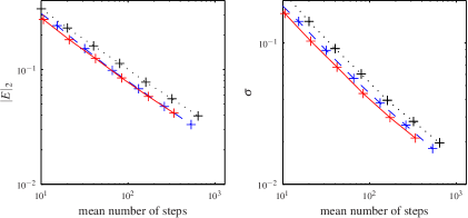
Figure 2: For Eq. 5.9, (left) the sample mean of the maximum relative error $|E|_{2}$ and (right) standard deviation $\sigma$ of the error $E$ (see Eq. 5.10) against the mean number of steps taken (based on 5000 samples). We plot (dashed) Adaptive-I with $\alpha=0.5$, (solid) Adaptive-II with $\alpha=0.9$, and (dotted) fixed time-stepping Euler–Maruyama method.

figure]fig:a3

5.3 Experiments with adaptive algorithms

We now test Adaptive-I and Adaptive-II with the Euler–Maruyama method using the following initial value problems:

$$dy=0.1y\,dt+1.2y\,dW(t),\qquad y(0)=1$$ (5.8)

and

$$dy=1.5y\,dt+2.4y\,dW(t),\qquad y(0)=1.$$ (5.9)

Here, $d=m=1$ and $W(t)$ is a standard Brownian motion. We integrate both equations numerically with the Euler–Maruyama method on the interval $[0,T]=[0,1]$ and compare the result with the exact solution (geometric Brownian motion). In this example, the drift and diffusion functions $g_{j}(y)$ are linear and unbounded. In the experiments, we replace $\left\|\mathchoice{\raisebox{0.0pt}{$\displaystyle{\vphantom{\bigm{|}}\mathopen{}q_{ij}(y_{k})}$}}{\smash{q_{ij}(y_{k})}}{q_{ij}(y_{k})}{q_{ij}(y_{k})}\right\|$ in Eqs. 5.1 and 5.2 with $\min\left\{\mathchoice{\raisebox{0.0pt}{$\displaystyle{\vphantom{\bigm{|}}\mathopen{}\left\|\mathchoice{\raisebox{0.0pt}{$\displaystyle{\vphantom{\bigm{|}}\mathopen{}q_{ij}(y_{k})}$}}{\smash{q_{ij}(y_{k})}}{q_{ij}(y_{k})}{q_{ij}(y_{k})}\right\|,100}$}}{\left\|\mathchoice{\raisebox{0.0pt}{$\displaystyle{\vphantom{\bigm{|}}\mathopen{}q_{ij}(y_{k})}$}}{\smash{q_{ij}(y_{k})}}{q_{ij}(y_{k})}{q_{ij}(y_{k})}\right\|,100}{\left\|\mathchoice{\raisebox{0.0pt}{$\displaystyle{\vphantom{\bigm{|}}\mathopen{}q_{ij}(y_{k})}$}}{\smash{q_{ij}(y_{k})}}{q_{ij}(y_{k})}{q_{ij}(y_{k})}\right\|,100}{\left\|\mathchoice{\raisebox{0.0pt}{$\displaystyle{\vphantom{\bigm{|}}\mathopen{}q_{ij}(y_{k})}$}}{\smash{q_{ij}(y_{k})}}{q_{ij}(y_{k})}{q_{ij}(y_{k})}\right\|,100}\right\}$; this ensures the time steps do not become too small.

For Adaptive-I, time steps and Brownian increments are generated using the method of (Milstein & Tretyakov,, 1999). For Adaptive-II, we’d like to sample from an exit time problem on the domain shown in Figure 1. We use the following approximate algorithm to sample from this distribution: Let $R$ denote the shaded region in Figure 1 for a given $\alpha$ and $h$. Choose a parameter $\beta>0$.

1. Let $(\tau^{0},x^{0})=(0,0)$ and $k=0$.

2. Choose the largest $a_{1}$ such that $\{\tau^{k}\}\times[x^{k}-a_{1},x^{k}+a_{1}]\subset R$, and then the largest $a_{0}$ such that $[\tau^{k},\tau^{k}+a_{0}]\times[x^{k}-a_{1},x^{k}+a_{1}]\subset R$.

3. Use the algorithm of (Milstein & Tretyakov,, 1999) to find the first exit point $(\tau,W(\tau))$ from $[0,a_{0}]\times[-a_{1},a_{1}]$ of the process $(t,W(t))$.

4. Let $\tau^{k+1}=\tau^{k}+\tau$ and $x^{k+1}=x^{k}+W(\tau)$. If $\tau<\beta h$, stop and output $(\tau^{k+1},x^{k+1})$. Otherwise, increase $k$ and go to 2).

The output can be used as the time step and Brownian increment, which always belongs to the region $R$ but is unlikely to be an exit point. We apply this method with $\beta=1/10$ to implement Adaptive-II and the resulting distribution of steps taken is shown in Figure 5.

We compute the maximum relative error on the partition ${\cal T}$, defined by

$$E\coloneq\frac{1}{Z}\max_{\tau_{n}\in{\cal T}}|y_{n}-y(\tau_{n})|,\qquad\text{ where }Z\coloneq\max_{\tau_{n}\in\mathcal{T}}|y(\tau_{n})|.$$ (5.10)

For $M$ iid samples $E_{1},\dots,E_{M}$ of $E$, we plot

$$|E|_{2}\coloneq\left(\mathchoice{\raisebox{0.0pt}{$\displaystyle{\vphantom{\bigm{|}}\mathopen{}\sum_{j=1}^{M}E_{j}^{2}}$}}{\sum_{j=1}^{M}E_{j}^{2}}{\sum_{j=1}^{M}E_{j}^{2}}{\sum_{j=1}^{M}E_{j}^{2}}\right)^{1/2}$$

and the standard deviation $\sigma$ of $E_{1},\dots,E_{M}$ against the mean number of steps, using $M=5000$ samples in LABEL:fig:a3 and LABEL:fig:a4. The adaptive methods outperform the fixed time-stepping method in terms of mean error (when taken with the same mean number of steps) and a 20% reduction in error is observed using either adaptive algorithm. Furthermore, the adaptive methods, especially Adaptive-II, produce a narrower range of errors, as we find the standard deviation of the errors is smaller. Whilst this is encouraging, we are discounting the extra time involved in sampling the bounded diffusion and, as this algorithm is slow compared to sampling a Gaussian increment, the adaptive methods are not yet fully practical.

Two further plots are shown for Eq. 5.8. Figure 4 shows a scatter plot of the errors $E$ against the number of steps taken for the three methods. Figure 5 shows the mean and standard deviation of the number of steps used in the experiments for a set of $h$ values.

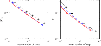
Figure 3: For Eq. 5.8, (left) $|E|_{2}$ and (right) standard deviation $\sigma$ of $E$ against the mean number of steps taken. We plot (dashed) Adaptive-I with $\alpha=0.5$, (solid) Adaptive-II with $\alpha=0.9$, and (dotted) fixed time-stepping Euler–Maruyama method.

figure]fig:a4

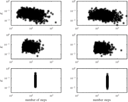
Figure 4: Plots of the relative error $E$ against number of steps taken $N$ for 100 samples of the approximation to Eq. 5.8 for (top) Adaptive-I with $\alpha=0.5$, (middle) Adaptive-II with $\alpha=0.9$, and (bottom) fixed time-stepping Euler–Maruyama.

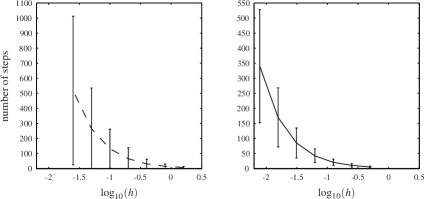
Figure 5: Mean number of steps with error bars indicating one standard deviation for (left) Adaptive-I with $\alpha=0.5$ and (right) Adaptive-II with $\alpha=0.9$ applied to Eq. 5.8.

6 Conclusion

We presented a new proof of pathwise convergence for numerical approximation of SDEs, which avoids the need to prove the $p$th-mean error converges at a polynomial rate. This requires two pathwise assumptions: first, a Lipschitz type assumption of the deviation of the sample path of the solution from its initial data and, second, a pathwise bound on the sum of the truncation errors. The proof of the pathwise-convergence theorem uses no probabilistic arguments. We showed how to apply the theorem to the Euler–Maruyama method with fixed time-stepping. We also introduced two adaptive time-stepping methods, motivated by the truncation error sum condition. To complete these proofs and verify the assumptions of the pathwise-convergence theorem, we do use probabilistic arguments and estimate moments and apply the Borel–Cantelli lemma. The main advantage of this approach is that more detailed constants are gained and we are able to find a tighter error bound for the adaptive methods. Computations with SDEs usually work by computing paths, even if the quantity of interest is an average or exit time, and the pathwise condition on the truncation error sum is a convenient framework for studying adaptive methods.

Some experiments were shown with geometric Brownian motion using a method of (Milstein & Tretyakov,, 1999) for bounded diffusions to generate the appropriate time steps and Brownian increments. For a given mean number of time steps, the errors are smaller and show less variation than for fixed time-stepping. This extra accuracy, which does not change the rate of convergence, requires sampling bounded diffusions rather than diffusions over fixed time-steps (iid Gaussian random variables) and this makes the algorithm expensive to implement. Finding a fast method for sampling bounded diffusions is a key point to be addressed in future research.

Appendix A Useful results

The first result concerns the regularity of sample paths and gives a large class of SDEs where Assumption 3.1 holds.

Lemma A.1.

If ${g}_{j}\in\mathrm{C}_{\mathrm{b}}^{3}({}^{d},{}^{d})$, then the solution $y(t;s,{z})$ of Eq. 1.1 satisfies Assumption 3.1.

Proof.

Fix $\epsilon>0$. Let ${x}(t;s,{z})\coloneq{y}(t;s,{z})-{z}$ for ${z}\in{}^{d}$ and $0\leq s,t\leq T$. Then, ${x}(t;s,z)$ satisfies

$$d{x}=d{y}=\sum_{j=0}^{m}g_{j}({y})\,dW^{j}(t)=\sum_{j=0}^{m}g_{j}({x}+{z})\,dW^{j}(t),\qquad{x}(s;s,{z})=0$$

and ${x}(t;s,{z}^{i})$ for $i=1,2$ are two solutions of an SDE with modified vector fields ${V}_{j}^{i}({q})={g}_{j}({q}+{z}^{i})$. Then, (Friz & Victoir,, 2010, Theorem 10.26) gives

$$\left\|\mathchoice{\raisebox{0.0pt}{$\displaystyle{\vphantom{\bigm{|}}\mathopen{}{x}(t;s,{z}^{1})-{x}(t;s,{z}^{2})}$}}{\smash{{x}(t;s,{z}^{1})-{x}(t;s,{z}^{2})}}{{x}(t;s,{z}^{1})-{x}(t;s,{z}^{2})}{{x}(t;s,{z}^{1})-{x}(t;s,{z}^{2})}\right\|\leq C|t-s|^{1/2-\epsilon}\max_{j}\left\|\mathchoice{\raisebox{0.0pt}{$\displaystyle{\vphantom{\bigm{|}}\mathopen{}V^{1}_{j}-V^{2}_{j}}$}}{\smash{V^{1}_{j}-V^{2}_{j}}}{V^{1}_{j}-V^{2}_{j}}{V^{1}_{j}-V^{2}_{j}}\right\|_{\mathrm{C}_{\mathrm{b}}^{2}}$$

for some $C$ dependent on the sample path of $W^{j}(t)$. Because $g_{j}\in\mathrm{C}_{\mathrm{b}}^{3}({}^{d},{}^{d})$, it is clear that $\left\|\mathchoice{\raisebox{0.0pt}{$\displaystyle{\vphantom{\bigm{|}}\mathopen{}V^{1}_{j}-V^{2}_{j}}$}}{\smash{V^{1}_{j}-V^{2}_{j}}}{V^{1}_{j}-V^{2}_{j}}{V^{1}_{j}-V^{2}_{j}}\right\|_{\mathrm{C}_{\mathrm{b}}^{2}}\leq\left\|\mathchoice{\raisebox{0.0pt}{$\displaystyle{\vphantom{\bigm{|}}\mathopen{}g_{j}}$}}{\smash{g_{j}}}{g_{j}}{g_{j}}\right\|_{\mathrm{C}_{\mathrm{b}}^{3}}\left\|\mathchoice{\raisebox{0.0pt}{$\displaystyle{\vphantom{\bigm{|}}\mathopen{}{z}^{1}-{z}^{2}}$}}{\smash{{z}^{1}-{z}^{2}}}{{z}^{1}-{z}^{2}}{{z}^{1}-{z}^{2}}\right\|$ and hence

$$\left\|\mathchoice{\raisebox{0.0pt}{$\displaystyle{\vphantom{\bigm{|}}\mathopen{}\left(\mathchoice{\raisebox{0.0pt}{$\displaystyle{\vphantom{\bigm{|}}\mathopen{}{y}(t;s,{z}^{1})-{z}^{1}}$}}{{y}(t;s,{z}^{1})-{z}^{1}}{{y}(t;s,{z}^{1})-{z}^{1}}{{y}(t;s,{z}^{1})-{z}^{1}}\right)-\left(\mathchoice{\raisebox{0.0pt}{$\displaystyle{\vphantom{\bigm{|}}\mathopen{}{y}(t;s,{z}^{2})-{z}^{2}}$}}{{y}(t;s,{z}^{2})-{z}^{2}}{{y}(t;s,{z}^{2})-{z}^{2}}{{y}(t;s,{z}^{2})-{z}^{2}}\right)}$}}{\smash{\left(\mathchoice{\raisebox{0.0pt}{$\displaystyle{\vphantom{\bigm{|}}\mathopen{}{y}(t;s,{z}^{1})-{z}^{1}}$}}{{y}(t;s,{z}^{1})-{z}^{1}}{{y}(t;s,{z}^{1})-{z}^{1}}{{y}(t;s,{z}^{1})-{z}^{1}}\right)-\left(\mathchoice{\raisebox{0.0pt}{$\displaystyle{\vphantom{\bigm{|}}\mathopen{}{y}(t;s,{z}^{2})-{z}^{2}}$}}{{y}(t;s,{z}^{2})-{z}^{2}}{{y}(t;s,{z}^{2})-{z}^{2}}{{y}(t;s,{z}^{2})-{z}^{2}}\right)}}{\left(\mathchoice{\raisebox{0.0pt}{$\displaystyle{\vphantom{\bigm{|}}\mathopen{}{y}(t;s,{z}^{1})-{z}^{1}}$}}{{y}(t;s,{z}^{1})-{z}^{1}}{{y}(t;s,{z}^{1})-{z}^{1}}{{y}(t;s,{z}^{1})-{z}^{1}}\right)-\left(\mathchoice{\raisebox{0.0pt}{$\displaystyle{\vphantom{\bigm{|}}\mathopen{}{y}(t;s,{z}^{2})-{z}^{2}}$}}{{y}(t;s,{z}^{2})-{z}^{2}}{{y}(t;s,{z}^{2})-{z}^{2}}{{y}(t;s,{z}^{2})-{z}^{2}}\right)}{\left(\mathchoice{\raisebox{0.0pt}{$\displaystyle{\vphantom{\bigm{|}}\mathopen{}{y}(t;s,{z}^{1})-{z}^{1}}$}}{{y}(t;s,{z}^{1})-{z}^{1}}{{y}(t;s,{z}^{1})-{z}^{1}}{{y}(t;s,{z}^{1})-{z}^{1}}\right)-\left(\mathchoice{\raisebox{0.0pt}{$\displaystyle{\vphantom{\bigm{|}}\mathopen{}{y}(t;s,{z}^{2})-{z}^{2}}$}}{{y}(t;s,{z}^{2})-{z}^{2}}{{y}(t;s,{z}^{2})-{z}^{2}}{{y}(t;s,{z}^{2})-{z}^{2}}\right)}\right\|\leq C|t-s|^{1/2-\epsilon}\left\|\mathchoice{\raisebox{0.0pt}{$\displaystyle{\vphantom{\bigm{|}}\mathopen{}{z}^{1}-{z}^{2}}$}}{\smash{{z}^{1}-{z}^{2}}}{{z}^{1}-{z}^{2}}{{z}^{1}-{z}^{2}}\right\|,$$

for all ${z}^{1},{z}^{2}\in{}^{d}$ and $0\leq s,t\leq T$. This is Assumption 3.1. ∎

For a stochastic process $Y(t)$, the modulus of continuity

$$\omega_{Y}(h)\coloneq\sup_{t,s\in[0,T],\;|t-s|\leq h}\left\|\mathchoice{\raisebox{0.0pt}{$\displaystyle{\vphantom{\bigm{|}}\mathopen{}{Y}(t)-{Y}(s)}$}}{\smash{{Y}(t)-{Y}(s)}}{{Y}(t)-{Y}(s)}{{Y}(t)-{Y}(s)}\right\|,\qquad h>0.$$

The following result examines the modulus of continuity when $Y$ is an Itô integral and is applied to the truncation error in order to derive Assumption 3.2.

Proposition A.2.

Let

$${Y}(t)=\int_{0}^{t}{q}_{0}(s)\,ds+\sum_{j=1}^{m}\int_{0}^{t}{q}_{j}(s)\,dW^{j}(s)$$

for predictable processes $\{{q}_{j}(s)\colon s\in[0,T]\}$. Consider random variables $\zeta,\xi$ such that, for some $p\geq 1$ and $K,\mu>0$,

$$\mathbb{E}\left[\mathchoice{\raisebox{0.0pt}{$\displaystyle{\vphantom{\bigm{|}}\mathopen{}|\zeta|^{p}}$}}{|\zeta|^{p}}{|\zeta|^{p}}{|\zeta|^{p}}\right]\leq K\quad\text{ and }\quad\mathbb{E}\left[\mathchoice{\raisebox{0.0pt}{$\displaystyle{\vphantom{\bigm{|}}\mathopen{}|\xi|^{p/2+\mu}}$}}{|\xi|^{p/2+\mu}}{|\xi|^{p/2+\mu}}{|\xi|^{p/2+\mu}}\right]\leq K,$$

and such that, for $0\leq s<t\leq T$,

$$\int_{s}^{t}\left\|\mathchoice{\raisebox{0.0pt}{$\displaystyle{\vphantom{\bigm{|}}\mathopen{}{q}_{0}(r)}$}}{\smash{{q}_{0}(r)}}{{q}_{0}(r)}{{q}_{0}(r)}\right\|\,dr\leq\zeta\;\sqrt{|t-s|\log(2T/|t-s|)},\qquad\sum_{j=1}^{m}\int_{s}^{t}\left\|\mathchoice{\raisebox{0.0pt}{$\displaystyle{\vphantom{\bigm{|}}\mathopen{}{q}_{j}(r)}$}}{\smash{{q}_{j}(r)}}{{q}_{j}(r)}{{q}_{j}(r)}\right\|^{2}\,dr\leq\xi\;|t-s|.$$

Then, for any $0<\epsilon<1/2$, there exists a random variable $C_{\epsilon}\in L^{p}(\Omega)$ such that

$$\omega_{Y}(h)\leq C_{\epsilon}h^{1/2-\epsilon}\qquad\text{for all $s,t\in[0,T]$}$$

and $\left\|\mathchoice{\raisebox{0.0pt}{$\displaystyle{\vphantom{\bigm{|}}\mathopen{}C_{\epsilon}}$}}{\smash{C_{\epsilon}}}{C_{\epsilon}}{C_{\epsilon}}\right\|_{L^{p}(\Omega)}$ depends only on $\epsilon,\mu,p,K,T$ and is independent of $q_{j}$.

Proof.

Under these conditions, Fischer & Nappo, (2009) tell us there exists $C>0$ depending only on $p,\mu,$ and $K$ such that

$$\left\|\mathchoice{\raisebox{0.0pt}{$\displaystyle{\vphantom{\bigm{|}}\mathopen{}\omega_{Y}(h)}$}}{\smash{\omega_{Y}(h)}}{\omega_{Y}(h)}{\omega_{Y}(h)}\right\|_{L^{p}(\Omega)}\leq C\sqrt{h\log(2T/h)}.$$

Then, for $\epsilon>0$, there exists a $C_{\epsilon}\in L^{p}(\Omega)$ such that $\omega_{Y}(h)\leq C_{\epsilon}h^{1/2-\epsilon}$ and hence

$$|Y(s)-Y(t)|\leq C_{\epsilon}|s-t|^{1/2-\epsilon},\qquad s,t\in[0,T].$$

The $L^{p}(\Omega)$ norm of $C_{\epsilon}$ is bounded uniformly in $\epsilon,\mu,$ and $K$, as required. ∎

The following is a consequence of the well-known Azuma inequality (Azuma,, 1967; DasGupta,, 2011).

Lemma A.3.

Let $Y_{i}$ be a sequence of scalar random variables with $|Y_{i}|\leq{\mkern 2.0mu\overline{\mkern-2.0mu{Y}\mkern 1.0mu\mkern-2.0mu}\mkern 2.0mu\mkern-1.0mu}{}$ a.s for a constant ${\mkern 2.0mu\overline{\mkern-2.0mu{Y}\mkern 1.0mu\mkern-2.0mu}\mkern 2.0mu\mkern-1.0mu}{}$. Suppose that $\mathbb{E}\left[\mathchoice{\raisebox{0.0pt}{$\displaystyle{\vphantom{\bigm{|}}\mathopen{}Y_{i}|Y_{0},\dots,Y_{i-1}}$}}{Y_{i}|Y_{0},\dots,Y_{i-1}}{Y_{i}|Y_{0},\dots,Y_{i-1}}{Y_{i}|Y_{0},\dots,Y_{i-1}}\right]=0$ a.s. for $i=1,\dots,n$. Let $S_{n}=Y_{1}+\dots+Y_{n}$. Then, for $\lambda>0$,

$$\mathbb{P}\left(\mathchoice{\raisebox{0.0pt}{$\displaystyle{\vphantom{\bigm{|}}\mathopen{}|S_{n}-S_{k}|\geq\lambda}$}}{|S_{n}-S_{k}|\geq\lambda}{|S_{n}-S_{k}|\geq\lambda}{|S_{n}-S_{k}|\geq\lambda}\right)\leq 2\exp\left(\mathchoice{\raisebox{0.0pt}{$\displaystyle{\vphantom{\bigm{|}}\mathopen{}-\frac{\lambda^{2}}{2(n-k){\mkern 2.0mu\overline{\mkern-2.0mu{Y}\mkern 1.0mu\mkern-2.0mu}\mkern 2.0mu\mkern-1.0mu}{}^{2}}}$}}{-\frac{\lambda^{2}}{2(n-k){\mkern 2.0mu\overline{\mkern-2.0mu{Y}\mkern 1.0mu\mkern-2.0mu}\mkern 2.0mu\mkern-1.0mu}{}^{2}}}{-\frac{\lambda^{2}}{2(n-k){\mkern 2.0mu\overline{\mkern-2.0mu{Y}\mkern 1.0mu\mkern-2.0mu}\mkern 2.0mu\mkern-1.0mu}{}^{2}}}{-\frac{\lambda^{2}}{2(n-k){\mkern 2.0mu\overline{\mkern-2.0mu{Y}\mkern 1.0mu\mkern-2.0mu}\mkern 2.0mu\mkern-1.0mu}{}^{2}}}\right).$$

References

- Azuma, (1967) Azuma, Kazuoki. 1967. Weighted sums of certain dependent random variables. Tôhoku Math. J. (2), 19, 357–367.
- DasGupta, (2011) DasGupta, Anirban. 2011. Probability for Statistics and Machine Learning. Springer Texts in Statistics. Springer.
- Davie, (2007) Davie, A. M. 2007. Differential equations driven by rough paths: an approach via discrete approximation. Appl. Math. Res. Express., 2, 40.
- Fischer & Nappo, (2009) Fischer, M., & Nappo, G. 2009. On the moments of the modulus of continuity of Itô processes. Stochastic Analysis and Applications, 28(1), 103–122.
- Friz & Victoir, (2010) Friz, Peter K., & Victoir, Nicolas B. 2010. Multidimensional Stochastic Processes as Rough Paths: Theory and Applications. Cambridge University Press.
- Gaines & Lyons, (1997) Gaines, J. G., & Lyons, T. J. 1997. Variable step size control in the numerical solution of stochastic differential equations. SIAM J. Appl. Math., 57(5), 1455–1484.
- Gyöngy, (1998) Gyöngy, István. 1998. A note on Euler’s approximations. Potential Anal., 8(3), 205–216.
- Kloeden & Neuenkirch, (2007) Kloeden, P. E., & Neuenkirch, A. 2007. The pathwise convergence of approximation schemes for stochastic differential equations. LMS J. Comput. Math., 10, 235–253.
- Kloeden & Platen, (1992) Kloeden, Peter E., & Platen, Eckhard. 1992. Numerical Solution of Stochastic Differential Equations. Applications of Mathematics, no. 23.
- Milstein, (1995) Milstein, G. N. 1995. The Numerical Integration of Stochastic Differential Equations. Kluwer.