From Hodge Index Theorem to the number of points of curves over finite fields

Abstract

We push further the classical proof of Weil upper bound for the number of rational points of an absolutely irreducible smooth projective curve $X$ over a finite field in term of euclidean relationships between the Neron Severi classes in $X\times X$ of the graphs of iterations of the Frobenius morphism. This allows us to recover Ihara’s bound, which can be seen as a second order Weil upper bound, to establish a new third order Weil upper bound, and using magma to produce numerical tables for higher order Weil upper bounds. We also give some interpretation for the defect of exact recursive towers, and give several new bounds for points of curves in relative situation $X\rightarrow Y$.

AMS classification : 11G20, 14G05, 14G15, 14H99.

Keywords : Curves over a finite field, rational point, Weil bound.

Introduction

Let $X$ be an absolutely irreducible smooth projective curve defined over the finite field ${\mathbb{F}}_{q}$ with $q$ elements. The classical proof of Weil Theorem for the number of $\mathbb{F}_{q}$-rational points $\sharp X({\mathbb{F}}_{q})$ rests upon Castelnuovo identity [Wei48], a corollary of Hodge index Theorem for the smooth algebraic surface $X\times X$. The intent of this article is to push further this viewpoint by forgetting Castelnuovo Theorem. We come back to the consequence of Hodge index Theorem that the intersection pairing on the Neron Severi space $\operatorname{NS}(X\times X)_{\mathbb{R}}$ is anti-euclidean on the orthogonal complement ${\mathcal{E}}_{X}$ of the trivial plane generated by the horizontal and vertical classes. Thus, the opposite $\left\langle\cdot,\cdot\right\rangle$ of the intersection pairing endows ${\mathcal{E}}_{X}$ with a structure of euclidean space. Section 1 is devoted to few useful scalar products computations.

In section 2, we begin by giving a proof of Weil inequality which is, although equivalent in principle, different in presentation than the usual one using Castelnuovo Theorem given for instance in [Har77, exercice 1.9, 1.10 p. 368] or in [Sha94, exercises 8, 9, 10 p. 251]). We prove that Weil bound follows from Cauchy-Schwartz inequality for the orthogonal projections onto ${\mathcal{E}}_{X}$ of the diagonal class $\Gamma^{0}$ and the class $\Gamma^{1}$ of the graph of the Frobenius morphism on $X$.

The benefit of using Cauchy-Schwartz instead of Castelnuovo is the following. We do not know what can be a Castelnuovo identity for more than two Neron Severi classes, while we do know what is Cauchy-Schwartz for any number of vectors. It is well-known that Cauchy-Schwartz between two vectors is the non-negativity of their $2\times 2$ Gram determinant. Hence, we are cheered on investigating the consequences of the non-negativity of larger Gram determinants involving the Neron Severi classes $\Gamma^{k}$ of the graphs of the $k$-th iterations of the Frobenius morphism.

For the family $\Gamma^{0},\Gamma^{1},\Gamma^{2}$, we recover the well known Ihara bound [Iha81] which improves Weil bound for curves of genus greater than $g_{2}=\frac{\sqrt{q}(\sqrt{q}-1)}{2}$, a constant appearing very naturally with this viewpoint in section 2.5.2, especialy looking at figure 1 in section 2.5.2. It follows that the classical Weil bound can be seen as a first order Weil bound, in that it comes from the euclidean constraints between $\Gamma^{0}$ and $\Gamma^{1}$, while the Ihara bound can be seen as a second order Weil bound, in that it comes from euclidean constraints between $\Gamma^{0}$, $\Gamma^{1}$ and $\Gamma^{2}$. Moreover this process can be pushed further: by considering the family $\Gamma^{0},\Gamma^{1},\Gamma^{2}$ and $\Gamma^{3}$, we obtain a new third order Weil bound (Theorem 18), which improves the Ihara bound for curves of genus greater than another constant $g_{3}=\frac{\sqrt{q}(q-1)}{\sqrt{2}}$.

The more the genus increases, the more the Weil bound should be chosen of high order in order to be optimal. Therefore it is useful to compute higher order Weil bounds. Unfortunately, establishing them explicitely requires the resolution of high degree one variable polynomial equations over ${\mathbb{R}}$. For instance, the usual Weil bound requires the resolution of a degree one equation, Ihara and the third order Weil bounds require the resolution of second order equations, while fourth and fifth order Weil bounds require the resolution of third degree equations, and so on. Moreover, a glance at Ihara second order Weil bound and at our explicit third order Weil bound will convince the reader that they become more and more ugly as the order increase.

Hence, we give up the hope to establish explicit formulae for the Weil bounds of order from 4. We then turn to a more algorithmic point of view. We use an algorithm which, for a given genus $g$ and a given field size $q$, returns the best upper order Weil bound for the number of ${\mathbb{F}}_{q}$-rational points of a genus $g$ curve, together with the corresponding best order $n$. The validity of this algorithm requires some results proved in the second section. In the figure below, we represent the successive Weil bounds (in logarithmic scales) of order from $1$ to $5$. Note that taking into account the logarithmic scale for the $y$-axis, higher order Weil bounds become significantly better than usual Weil’s one.

Weil bounds of order $1$ to $5$ for $\sharp X(\mathbb{F}_{q})$ (here for $q=2$). Note that the $y$ axis is logarithmic. For small genus, red usual first order Weil bound is the best one. Then from genus $g_{2}=\frac{\sqrt{q}(\sqrt{q}-1)}{2}$, yellow Ihara’s second order Weil bound becomes the best, up to the genus $g_{3}=\frac{\sqrt{q}(q-1)}{\sqrt{2}}$ where green third order weil bound becomes the best. From some genus $g_{4}$, light blue fourth order Weil bound is the best up to some genus $g_{5}$, where dark blue fifth order Weil bound becomes better, and so on. Here, we have chosen $q=2$, for which the genera $g_{2},g_{3},g_{4},g_{5}$ are particularly small, respectively about $0.3,1,2.35$ and $4.67$. This means for instance that the best bound for $q=2$ and $g=3,4$ is the fourth order one!

In order to illustrate the efficiency of our algorithm, we display in section 2.6.3 a numerical table.

We acknowledge that for any pair $(g,q)$ we have tested, a comparison of our numerical results with the table given on the website http://www.manypoints.org/ reveals that we always recover the very same numerical upper bound for $N_{q}(g)$ than those coming from Oesterlé bounds! We were not been able to understand this experimental observation.

Nevertheless, we think that the viewpoint introduced in this article is preferable to Osterlé’s one. First, our viewpoint is more conceptual in nature. Any constraints we use to obtain our bounds come in a quite pleasant way either from algebraic-geometry or from arithmetic, as explained in the introduction of section 2 in which we outline our approach. We think moreover that the graph displayed just above is very satisfying. Second, the viewpoint introduced in this article is perfectly adapted to the study of bounds for the numbers of rational points. As the reader can see, many known results can be understood with this viewpoint -even asymptotical ones, and new results can be proved. We are pretty sure that we have not extracted all potential outcomes of this viewpoint. Third, new questions can be raised from this viewpoint. We propose a few in Section 4.

To conclude Section 2, we push to the infinite-order Weil bound using the non-negativity of the Gram determinants of any orders, which imply that some symmetric matrix is semi-definite positive. Applied to some very simple vector, this lead us to Theorem 22, a stronger form of [Tsf92] Tsfasman bound in that it gives a new interpretation for the defect of an exact tower as a limit of nice euclidean vectors in $\left({\mathcal{E}},\left\langle\cdot,\cdot\right\rangle\right)$.

In Section 3, we study the relative situation. Given a finite morphism $f:X\to Y$ between two absolutely irreducible smooth projective curves defined over ${\mathbb{F}}_{q}$, the pull-back functor on divisors from the bottom algebraic surface $Y\times Y$ to the top one $X\times X$ induces a map from the Neron Severi space $\operatorname{NS}(Y\times Y)_{\mathbb{R}}$ to $\operatorname{NS}(X\times X)_{\mathbb{R}}$. Restricting this map to the subspaces ${\mathcal{F}}_{X}$ and ${\mathcal{F}}_{Y}$ generated by the classes of the graphs of iterations of the Frobenius morphisms, and after a suitable normalization (which differs from the normalization chosen in Section 2), we prove that it becomes an isometric embedding. We thus have an orthogonal decomposition ${\mathcal{F}}_{X}={\mathcal{F}}_{Y}^{*}\oplus{\mathcal{F}}_{X/Y}$, involving a relative subspace ${\mathcal{F}}_{X/Y}$ of ${\mathcal{F}}_{X}$.

Now, Cauchy-Schwartz inequality applied to the orthogonal projections of $\Gamma^{0}_{X}$ and $\Gamma^{1}_{X}$ on the relative space ${\mathcal{F}}_{X/Y}$ is equivalent to the well known relative Weil bound that $|\sharp X({\mathbb{F}}_{q})-\sharp Y({\mathbb{F}}_{q})|\leq 2(g_{X}-g_{Y})\sqrt{q}$.

With regard to higher orders relative Weil bounds, we encounter a difficulty since the arithmetical constraints $\sharp X({\mathbb{F}}_{q^{r}})-\sharp Y({\mathbb{F}}_{q^{r}})\geq\sharp X({\mathbb{F}}_{q})-\sharp Y({\mathbb{F}}_{q})$ for $r\geq 2$, similar to that used in Section 2 does not hold true! Hence, the only constraints we are able to use are the non-negativity of Gram determinants. This lead to an inequality relating the quantities $\sharp X({\mathbb{F}}_{q^{r}})-\sharp Y({\mathbb{F}}_{q^{r}})$ (corollary 29). We also prove a bound involving four curves in a cartesian diagram under some smoothness assumption (Theorem 33).

As stated above, we end this article by a very short Section 4, in which we raise a few questions.

1 The euclidean space $\left({\mathcal{E}},\left\langle\cdot,\cdot\right\rangle\right)$

Let $X$ be an absolutely irreducible smooth projective curve defined over the finite field $\mathbb{F}_{q}$ with $q$ elements. We consider the Neron-Severi space $\operatorname{NS}(X\times X)_{\mathbb{R}}=\operatorname{NS}(X\times X)\otimes_{\mathbb{Z}}\mathbb{R}$ of the smooth surface $X\times X$. It is well known that the intersection product of two divisors $\Gamma$ and $\Gamma^{\prime}$ on $X\times X$ induces a symmetric bilinear form on $\operatorname{NS}(X\times X)_{\mathbb{R}}$, whose signature is given by the following Hodge Index Theorem (e.g. [Har77]).

Theorem 1 (Hodge index Theorem).

The intersection pairing is non-degenerate on the space $\operatorname{NS}(X\times X)_{\mathbb{R}}$, and is definite negative on the orthogonal supplement of any ample divisor.

Let $H=X\times\{*\}$ and $V=\{*\}\times X$ be the horizontal and vertical classes on $X\times X$. Their intersection products are given by $H\cdot H=V\cdot V=0$ and $H\cdot V=1$. The restriction of the intersection product to $\operatorname{Vect}(H,V)$ has thus signature $(1,-1)$. Moreover $\operatorname{Vect}(H,V)\cap\operatorname{Vect}(H,V)^{\perp}=\{0\}$. By non-degeneracy, this gives rise to an orthogonal decomposition $\operatorname{NS}(X\times X)_{\mathbb{R}}=\operatorname{Vect}(H,V)\oplus\operatorname{Vect}(H,V)^{\perp}$. Let $p$ be the orthogonal projection onto the non-trivial part $\operatorname{Vect}(H,V)^{\perp}$, given by

$$\begin{array}[]{rccl}p:&\operatorname{NS}(X\times X)_{\mathbb{R}}&\longrightarrow&\operatorname{Vect}(H,V)^{\perp}\\ &\Gamma&\longmapsto&\Gamma-(\Gamma\cdot V)H-(\Gamma\cdot H)V.\end{array}$$ (1)

Since $H+V$ is ample, the intersection pairing is definite negative on $\operatorname{Vect}(H,V)^{\perp}$ by Hodge index Theorem. Hence, $\operatorname{Vect}(H,V)^{\perp}$ can be turned into an euclidean space by defining a scalar product as the opposite of the intersection pairing.

Definition 2.

Let ${\mathcal{E}}=\operatorname{Vect}(H,V)^{\perp}$. We define on ${\mathcal{E}}$ a scalar product, denoted by $\left\langle\cdot,\cdot\right\rangle$, as

$$\left\langle\gamma,\gamma^{\prime}\right\rangle=-\gamma\cdot\gamma^{\prime},\qquad\forall\gamma,\gamma^{\prime}\in{\mathcal{E}}.$$

The associated norm on ${\mathcal{E}}$ is denoted by $\|\cdot\|$.

In the sequel of this article, all the computations will take place in the euclidean space $\left({\mathcal{E}},\left\langle\cdot,\cdot\right\rangle\right)$. To begin with, let us compute this pairing between the iterates of the Frobenius morphism.

Lemma 3.

Let $F:X\to X$ denotes the $q$-Frobenius morphism on $X$, and $F^{k}$ denotes the $k$-th iterate of $F$ for any $k\geq 0$, with the usual convention that $F^{0}=\operatorname{Id}_{X}$. We denote by $\Gamma^{k}$ the Neron Severi class of the graph of $F^{k}$. Then

$$\begin{cases}\left\langle p(\Gamma^{k}),p(\Gamma^{k})\right\rangle=2gq^{k}&\forall k\geq 0\\ \left\langle p(\Gamma^{k}),p(\Gamma^{{k+i}})\right\rangle=q^{k}\left((q^{i}+1)-\sharp X(\mathbb{F}_{q}^{i})\right)&\forall k\geq 0,\,\forall i\geq 1.\end{cases}$$

Proof — Since the morphism $F^{k}$ is a regular map of degree $q^{k}$, one has $\Gamma^{k}\cdot H=q^{k}$ and $\Gamma^{k}\cdot V=1$. Now, let $k\in\mathbb{N}$ and $i\in\mathbb{N}^{*}$. We consider the map $\pi=F^{k}\times\operatorname{Id}:X\times X\rightarrow X\times X$, which sends $(P,Q)$ to $(F^{k}(P),Q)$. We have $\pi^{*}(\Delta)=\Gamma^{k}$ and $\pi_{*}\left(\Gamma^{{k+i}}\right)=q^{k}\Gamma^{i}$, so that by projection formula for the proper morphism $\pi$:

$$\Gamma^{{k}}\cdot\Gamma^{{k+i}} =\pi^{*}(\Delta)\cdot\Gamma^{{k+i}}$$

$$=\Delta\cdot\pi_{*}\left(\Gamma^{{k+i}}\right)$$

$$=q^{k}\Delta\cdot\Gamma^{i}.$$

If $i\geq 1$, then $\Delta\cdot\Gamma^{i}=\sharp X(\mathbb{F}_{q^{i}})$. If $i=0$, then $\Gamma^{0}=\Delta$ and $\Delta\cdot\Gamma^{0}=\Delta^{2}=-2g$. The results follow since $p(\Gamma^{k})=\Gamma^{k}-H-q^{k}V$ by (1). $\square$

Remark – Of course, $\dim{\mathcal{E}}\leq\dim NS(X\times X)_{\mathbb{R}}-2\leq 4g^{2}$. But as the reader can check, we are working along this article only on the subspace ${\mathcal{F}}$ of ${\mathcal{E}}$ generated by the family $p(\Gamma^{k}),k\geq 0$. By ([Zar95] chapter VII, appendix of Mumford), any trivial linear combination of this family is equivalent to the triviality of the same linear combination of the family $\varphi_{\ell}^{k},k\geq 0$, of the iteration of the Frobenius endomorphism $\varphi_{\ell}$ on the Tate module $V_{\ell}(\hbox{Jac }X)$ for any prime $\ell\wedge q=1$. We deduce that for a given curve $X$ over $\mathbb{F}_{q}$ of genus $g$, we actually are working in an euclidean space ${\mathcal{F}}_{X}$ of dimension equal to the degree of the minimal polynomial of $\varphi_{\ell}$ on $V_{\ell}(\hbox{Jac }X)$.

2 Absolute bounds

We observe, as a consequence of Lemma 3, that the non-negativity

$$0 \leq\operatorname{Gram}(p(\Gamma^{0}),p(\Gamma^{1}))=\begin{vmatrix}2g&q+1-\sharp X(\mathbb{F}_{q})\\ q+1-\sharp X(\mathbb{F}_{q})&2gq\end{vmatrix}$$

$$=(2g\sqrt{q})^{2}-(q+1-\sharp X(\mathbb{F}_{q}))^{2}$$

is nothing else than Weil inequality. In this Section, we give other bounds using larger Gram determinants. For this purpose, we need preliminary notations, normalizations and results.

Normalizations in Section 2.1 play two parts. They ease many formulae and calculations. They also make obvious that several features of the problem, such as the Gram matrix $\operatorname{Gram}(p(\Gamma^{i});0\leq i\leq n)$, or the forthcoming $n$-th Weil domains $\mathcal{W}_{n}$, are essentially independent of $q$. The authors believe that these features deserve to be emphasized.

With regard to results, let $n\in\mathbb{N}^{*}$. To obtain the Weil bound of order $n$, let $X$ be an algebraic curve of genus $g$ defined over $\mathbb{F}_{q}$. We use both geometric and arithmetic facets of $X$ as follows. We define from $X$ in (4) a point $P_{n}(X)\in\mathbb{R}^{n}$, whose abscissa $x_{1}$ given in (3) is essentially the opposite of $\sharp X(\mathbb{F}_{q})$, hence have to be lower bounded. The algebraic-geometric facet of $X$ implies, thanks to Hodge index Theorem, that some Gram determinant involving the coordinates of $P_{n}(X)$ is non-negative. This is traduced on the point $P_{n}(X)$ in Lemma 12 in that it do lies inside some convex $n$-th Weil domain $\overline{\mathcal{W}}_{n}$, studied in Subsection 2.3. The arithmetic facet of $X$ is used via Ihara constraints, that for any $r\geq 2$ we have $\sharp X(\mathbb{F}_{q^{r}})\geq\sharp X(\mathbb{F}_{q})$. We then define in Subsection 2.4 the convex $n$-th Ihara domain $\mathcal{H}_{n}^{g}$ in genus $g$. We state in Proposition 16 that for any curve $X$ of genus $g$ defined over $\mathbb{F}_{q}$, we have $P_{n}(X)\in\overline{\mathcal{W}}_{n}\cap\mathcal{H}_{n}^{g}$. We are thus reduced to minimize the convex function $x_{1}$ on the convex domain $\overline{\mathcal{W}}_{n}\cap\mathcal{H}_{n}^{g}$. To this end, we establish in Subsection 2.4 the optimization criteria 17, decisive for the derivations of higher order Weil bounds.

This criteria is used to prove new bounds in Subsection 2.6. Finally, we obtain in Subsection 2.7 a refined form of Tsfasman upper bound for asymptoticaly exact towers.

2.1 The Gram matrix of the normalized classes of iterated Frobenius

In this Subsection, we choose to normalize the Neron-Severi classes of the iterated Frobenius morphisms as follows. For any $n\geq 1$, and any curve $X$ defined over $\mathbb{F}_{q}$ of genus $g\neq 0$, we define a point $P_{n}(X)\in\mathbb{R}^{n}$ whose $x_{i}$-coordinates is very closely related to $\sharp X(\mathbb{F}_{q^{i}})$.

Definition 4.

Let $X$ be an absolutely irreducible smooth projective curve defined over the finite field $\mathbb{F}_{q}$. For $k\in\mathbb{N}$, we put

$$\gamma^{k}=\frac{1}{\sqrt{2gq^{k}}}p(\Gamma^{k})\in{\mathcal{E}},$$ (2)

so that by Lemma 3 we have $\left\langle\gamma^{k},\gamma^{k}\right\rangle=1$. For $i\in\mathbb{N}^{*}$, we put

$$x_{i}\overset{\text{def.}}{=}\left\langle\gamma^{k},\gamma^{{k+i}}\right\rangle\overset{\text{lemma~{}\ref{Intersections}}}{=}\frac{(q^{i}+1)-\sharp X(\mathbb{F}_{q^{i}})}{2g\sqrt{q}^{i}}.$$ (3)

For any $n\geq 1$, we define the point

$$P_{n}(X)=(x_{1},\ldots,x_{n})\in\mathbb{R}^{n}.$$ (4)

Remark – Note first that $X$ is Weil-maximal if and only if $x_{1}=-1$, and is Weil minimal if and only if $x_{1}=1$. Second, that to give upper bounds for $\sharp X(\mathbb{F}_{q})$ amount to give lower bounds for $x_{1}$.

From this Definition 4 and Lemma 3, the Gram matrix of the family $\gamma^{0},\ldots,\gamma^{n}$ in ${\mathcal{E}}$ is

$$\operatorname{Gram}(\gamma^{0},\ldots,\gamma^{n})=\begin{pmatrix}1&x_{1}&\cdots&x_{n-1}&x_{n}\\ x_{1}&\ddots&\ddots&&x_{n-1}\\ \vdots&\ddots&\ddots&\ddots&\vdots\\ x_{n-1}&&\ddots&\ddots&x_{1}\\ x_{n}&x_{n-1}&\cdots&x_{1}&1\end{pmatrix}$$ (5)

2.2 Some identities involving Toeplitz matrices

The main result of this Subsection is Lemma 5, providing the existence of the factorization in Definition 6, in which the $G_{n}^{-}$ factor plays a fundamental part in the following of the article.

A symmetric Toeplitz matrix is a symmetric matrix whose entries $x_{i,j}$ depend only on $|i-j|$, that is are constant along the diagonals parallel to the main diagonal [HJ90, §0.9.7], that is

$$T_{n+1}(x_{0},x_{1},\ldots,x_{n})=\begin{pmatrix}x_{0}&x_{1}&\cdots&x_{n-1}&x_{n}\\ x_{1}&\ddots&\ddots&&x_{n-1}\\ \vdots&\ddots&\ddots&\ddots&\vdots\\ x_{n-1}&&\ddots&\ddots&x_{1}\\ x_{n}&x_{n-1}&\cdots&x_{1}&x_{0}\end{pmatrix}$$ (6)

The symmetric Toeplitz matrix is said to be normalized if $x_{0}=1$.

An Hankel matrix is a matrix whose entries $x_{i,j}$ depend only on $i+j$, that is are constant along the anti-diagonals parallel to the main anti-diagonal [HJ90, §0.9.8], that is

$$H_{n+1}(x_{0},x_{1},\ldots,x_{2n})=\begin{pmatrix}x_{0}&x_{1}&x_{2}&\cdots&x_{n}\\ x_{1}&\reflectbox{$\ddots$}&&\reflectbox{$\ddots$}&x_{n+1}\\ x_{2}&&\reflectbox{$\ddots$}&\reflectbox{$\ddots$}&\vdots\\ \vdots&\reflectbox{$\ddots$}&\reflectbox{$\ddots$}&&x_{2n-1}\\ x_{n}&x_{n+1}&\cdots&x_{2n-1}&x_{2n}\end{pmatrix}$$ (7)

Remark – It should be noticed that in this article, any matrix is indexed by its size, while this doesn’t hold for determinants, for instance see formulae (9) and  (10).

Lemma 5.

For any $n\geq 1$, we abbreviate $T_{n}(x_{0},\ldots,x_{n-1})$ by $T_{n}$. The determinant of this Toeplitz matrix factorizes as

$$\operatorname{Det}\left(T_{2n}\right)=\operatorname{Det}\left(T_{n}+H_{n}(x_{2n-1},\ldots,x_{1})\right)\times\operatorname{Det}\left(T_{n}-H_{n}(x_{2n-1},\ldots,x_{1})\right)$$

and

$$\operatorname{Det}\left(T_{2n+1}\right)=\operatorname{Det}\begin{pmatrix}T_{n}+H_{n}(x_{2n},\ldots,x_{2})&{}^{t}X_{n}\\ 2X_{n}&x_{0}\end{pmatrix}\times\operatorname{Det}\left(T_{n}-H_{n}(x_{2n},\ldots,x_{2})\right),$$

where $X_{n}=(x_{n},\ldots,x_{1})$.

Proof — Even size. The operations on the columns $C_{j}\leftarrow C_{j}+C_{2n-(j-1)}$ for $1\leq j\leq n$, followed by the operations on the lines $L_{n+i}\leftarrow L_{n+i}-L_{n-(i-1)}$ for $1\leq i\leq n$ lead to the determinant of a $2\times 2$ blocks upper triangular matrix whose value is the expected product.

Odd size. The operations on the columns $C_{j}\leftarrow C_{j}+C_{2n+1-(j-1)}$ for $1\leq j\leq n$, followed by the operations on the lines $L_{n+1+i}\leftarrow L_{n+1+i}-L_{n+1-i}$ for $1\leq i\leq n$ lead to the result in the same manner. $\square$

Definition 6.

For $n=0$, we put $G_{0}=G_{0}^{-}=G_{0}^{+}=1$, and for $n\geq 1$, we put

$$G_{n}(x_{1},\ldots,x_{n})\overset{\text{def.}}{=}\operatorname{Det}(T_{n+1}(1,x_{1},\ldots,x_{n}))\overset{\text{Lemma~{}\ref{lem_factorization}}}{=}G_{n}^{-}(x_{1},\ldots,x_{n})\times G_{n}^{+}(x_{1},\ldots,x_{n}),$$

where the last factorization is the one proved in Lemma 5 in the same order.

Remark – The determinant $G_{n}$ is the determinant of a matrix of size $n+1$. Note that for $n=2m+1$ odd, both $G_{n}^{-}$ and $G_{n}^{+}$ are polynomials of degree $m+1$ in $x_{1},\ldots,x_{n}$, while for $n=2m$ even, $G_{n}^{-}$ has degree $m+1$, while $G_{n}^{+}$ have degree $m$. We will see later in the article that Weil bound of order n for $\sharp X(\mathbb{F}_{q})$ depends heavily on the hypersurface $\{G_{n}^{-}=0\}$.

In order to raise any ambiguity and for later purpose, let us write down these determinants for $n=1,2$ and $3$:

$$G_{1}(x_{1}) =\begin{vmatrix}1&x_{1}\\ x_{1}&1\end{vmatrix}=\underbrace{(1+x_{1})}_{G_{1}^{-}(x_{1})}\times\underbrace{(1-x_{1})}_{G_{1}^{+}(x_{1})}$$ (8)

$$G_{2}(x_{1},x_{2}) =\begin{vmatrix}1&x_{1}&x_{2}\\ x_{1}&1&x_{1}\\ x_{2}&x_{1}&1\end{vmatrix}=\underbrace{\begin{vmatrix}1+x_{2}&x_{1}\\ x_{1}+x_{1}&1\end{vmatrix}}_{G_{2}^{-}(x_{1},x_{2})}\times\underbrace{(1-x_{2})}_{G_{2}^{+}(x_{1},x_{2})}$$ (9)

$$G_{3}(x_{1},x_{2},x_{3}) =\begin{vmatrix}1&x_{1}&x_{2}&x_{3}\\ x_{1}&1&x_{1}&x_{2}\\ x_{2}&x_{1}&1&x_{1}\\ x_{3}&x_{2}&x_{1}&1\end{vmatrix}=\underbrace{\begin{vmatrix}1+x_{3}&x_{1}+x_{2}\\ x_{1}+x_{2}&1+x_{1}\end{vmatrix}}_{G_{3}^{-}(x_{1},x_{2},x_{3})}\times\underbrace{\begin{vmatrix}1-x_{3}&x_{1}-x_{2}\\ x_{1}-x_{2}&1-x_{1}\end{vmatrix}}_{G_{3}^{+}(x_{1},x_{2},x_{3})}$$ (10)

Lemma 7.

For any $n\geq 1$ and $\epsilon=\pm$ or nothing, we abbreviate $G_{n}^{\epsilon}(x_{1},\ldots,x_{n})$ by $G_{n}^{\epsilon}$. Then one has

$$2G_{n}=G_{n-1}^{+}\times G_{n+1}^{-}+G_{n-1}^{-}\times G_{n+1}^{+}.$$

Proof — Let $S_{n+1}^{-}$ be the matrix obtained from $T_{n}$ by adding ${}^{t}(x_{n},\ldots,x_{1})$ to the first column, and $S_{n+1}^{+}$ be the matrix obtained from $T_{n}$ by removing ${}^{t}(x_{n},\ldots,x_{1})$ to the first column. Then by multilinearity, there exists a polynomial $R_{n}$ such that:

$$\operatorname{Det}\left(S_{n+1}^{-}\right)=G_{n}+R_{n}\quad\text{and}\quad\operatorname{Det}\left(S_{n+1}^{+}\right)=G_{n}-R_{n}.$$

On the other hand, using the same transformations as in the proof of Lemma 5, one get

$$\operatorname{Det}(S_{n+1}^{-})=G_{n-1}^{+}G_{n+1}^{-}\quad\text{and}\quad\operatorname{Det}(S_{n+1}^{+})=G_{n-1}^{-}G_{n+1}^{+}$$

Adding $\operatorname{Det}(S_{n+1}^{-})$ and $\operatorname{Det}(S_{n+1}^{+})$ allows us to conclude. $\square$

2.3 The domain of positive definite normalized Toeplitz matrices

In this Subsection, we study for any $n\geq 1$ some domain $\mathcal{W}_{n}\subset\mathbb{R}^{n}$, whose closure $\overline{\mathcal{W}}_{n}$ also plays a fundamental part in this article.

Definition 8.

Let $n\in{\mathbb{N}}^{*}$. We denote by $\mathcal{W}_{n}$ the set of $(x_{1},\ldots,x_{n})\in\mathbb{R}^{n}$, such that the symmetric normalized Toeplitz matrix $T_{n+1}(1,x_{1},\ldots,x_{n})$ is positive definite.

The domain $\mathcal{W}_{n}$ can be characterized in several useful ways.

Proposition 9.

For $n\geq 1$, the domain $\mathcal{W}_{n}$ is a convex subset of $\left]-1,1\right[^{n}$, which can be written as follows.

1. First, one has:

   $$\mathcal{W}_{n}=\left\{(x_{1},\ldots,x_{n})\in\mathbb{R}^{n}\mid G_{i}(x_{1},\ldots,x_{i})>0,\;\forall\;1\leq i\leq n\right\}.$$

2. Recursively, $\mathcal{W}_{1}=\left]-1,1\right[$ and for any $n\geq 2$

   $$\mathcal{W}_{n} =\left\{(x_{1},\ldots,x_{n-1},x_{n})\in\mathcal{W}_{n-1}\times\mathbb{R}\mid G_{n}(x_{1},\ldots,x_{n})>0\right\}$$

   $$=\left\{(x_{1},\ldots,x_{n-1},x_{n})\in\mathcal{W}_{n-1}\times\mathbb{R}\mid G_{n}^{-}(x_{1},\ldots,x_{n})>0\text{ and }G_{n}^{+}(x_{1},\ldots,x_{n})>0\right\}.$$

3. $\mathcal{W}_{n}$ is also the set of points between the graphs of two functions from $\mathcal{W}_{n-1}$ to $\mathbb{R}$: for $\varepsilon=\pm$, there exists a polynomial $\widetilde{G}_{n}^{\varepsilon}\in\mathbb{Q}[x_{1},\ldots,x_{n-1}]$, such that $G_{n}^{\epsilon}=-\epsilon G_{n-2}^{\epsilon}x_{n}+\epsilon\widetilde{G}_{n}$ and

   $$\mathcal{W}_{n}=\left\{(x_{1},\ldots,x_{n-1},x_{n})\in\mathcal{W}_{n-1}\times\mathbb{R}\mid\frac{\widetilde{G}^{-}_{n}(x_{1},\ldots,x_{n-1})}{G_{n-2}^{-}(x_{1},\ldots,x_{n-2})}<x_{n}<\frac{\widetilde{G}_{n}^{+}(x_{1},\ldots,x_{n-1})}{G_{n-2}^{+}(x_{1},\ldots,x_{n-2})}\right\}.$$

Proof — To prove the convexity, we remark that both sets of normalized symmetric Toeplitz matrices and of symmetric positive definite matrices are convex, so that $\mathcal{W}_{n}$ is convex. Moreover, $\mathcal{W}_{n}\subset\left]-1,1\right[^{n}$ because if $T_{n+1}(1,x_{1},\ldots,x_{n})$ is positive definite, then all its principal minors are positive. In particular, for any $1\leq i\leq n$, the $2\times 2$ minors $\left|\begin{smallmatrix}1&x_{i}\\ x_{i}&1\end{smallmatrix}\right|$ is positive.

Item (1) follows from the well known fact that an $n\times n$ symmetric matrix is definite positive if and only if all its $n$ leading principal minors (obtained by deleting the $i$ last rows and columns for $0\leq i\leq n-1$) are positive [HJ90, Theorem 7.2.5]. Hence, the first characterization of item (2) follows from item 1 . To prove the second characterization of item (2), we use Lemma 7 stating that $2G_{n-1}=G_{n-2}^{-}G_{n}^{+}+G_{n-2}^{+}G_{n}^{-}$. By induction, this allow us to prove that both factors are positive if, and only if, the product

$$G_{n}(x_{1},\ldots,x_{n})=G_{n}^{-}(x_{1},\ldots,x_{n})G_{n}^{+}(x_{1},\ldots,x_{n})$$

is positive for any $(x_{1},\ldots,x_{n-1})\in\mathcal{W}_{n-1}$.

To prove item (3), for $\epsilon=\pm$, formulae defining the polynomials $G_{n}^{\epsilon}$ in Lemma 5 and Definition 6 imply, developing along their first column and taking advantage of the very particular forms (6) and (7), that both polynomials have degree $1$ in $x_{n}$, of the form

$$G_{n}^{\epsilon}=-\epsilon G_{n-2}^{\epsilon}x_{n}+\varepsilon\widetilde{G}_{n}^{\epsilon}(x_{1},\ldots,x_{n-1})$$

for some $\widetilde{G}_{n}^{\epsilon}\in\mathbb{Q}[x_{1},\ldots,x_{n-1}]$. Since by item 2 we have $G_{n-2}^{\varepsilon}>0$, the set $\mathcal{W}_{n}$ is thus equal to the set of $(x_{1},\ldots,x_{n-1},x_{n})\in\mathcal{W}_{n-1}\times\mathbb{R}$, such that:

$$\frac{\widetilde{G}^{-}_{n}(x_{1},\ldots,x_{n-1})}{G_{n-2}^{-}(x_{1},\ldots,x_{n-2})}<x_{n}<\frac{\widetilde{G}_{n}^{+}(x_{1},\ldots,x_{n-1})}{G_{n-2}^{+}(x_{1},\ldots,x_{n-2})},$$

and the proof is complete. $\square$

The following Proposition is useful for later purpose in Section 2.6, where convexity plays a quite important part.

Proposition 10.

The locus $\{(x_{1},\ldots,x_{n})\in\mathcal{W}_{n-1}\times\mathbb{R}\mid G_{n}^{-}(x_{1},\ldots,x_{n})>0\}$ is convex, while the locus $\{(x_{1},\ldots,x_{n})\in\mathcal{W}_{n-1}\times\mathbb{R}\mid G_{n}^{+}(x_{1},\ldots,x_{n})>0\}$ is concave.

Proof — By item 3 of Proposition 9, $\mathcal{W}_{n}$ is the set of $(x_{1},\ldots,x_{n-1},x_{n})\in\mathcal{W}_{n-1}\times\mathbb{R}$ such that $x_{n}$ is between two functions from $\mathcal{W}_{n-1}$ to $\mathbb{R}$. By convexity of $\mathcal{W}_{n}$ from Proposition 9, the lower function must be concave has a function on $\mathcal{W}_{n-1}$ while the upper one must be convex. The Proposition follows easily. $\square$

The closure of $\mathcal{W}_{n}$ is given by the following Proposition.

Proposition 11.

The closure $\overline{\mathcal{W}}_{n}$ of $\mathcal{W}_{n}$ in $\mathbb{R}^{n}$ corresponds to the set of $(n+1)\times(n+1)$ normalized symmetric Toeplitz matrices which are positive semi definite. Moreover, we have

$$\overline{\mathcal{W}}_{n}=\left\{(x_{1},\ldots,x_{n})\in\mathbb{R}^{n}\mid G_{n,I}(x_{1},\ldots,x_{i})\geq 0,\;\forall I\subset\{0,1,\ldots,n\}\right\},$$

where, for $I\subset\{0,1,\ldots,n\}$, we denote by $G_{n,I}(x_{1},\ldots,x_{n})$ the principal minor of the normalized symmetric Toeplitz matrix $T_{n+1}(1,x_{1},\ldots,x_{n})$ obtained by deleting the lines and columns whose indices are not in $I$.

Proof — This is a consequence of the fact that a matrix is positive semi definite if and only if all the principal minors (the ones obtained by deleting the same subset of lines and columns) are non-negative (i.e. $\geq 0$) [HJ90, last exercise after Theorem 7.2.5]. $\square$

2.4 The curves locus

In this Subsection, we introduce Ihara’s constraints and the resulting $n$-Ihara domain $\mathcal{H}_{n}^{g}$ for genus g. We then gather the key results for the derivation of higher order Weil bounds. The first one is Proposition 16, the second one is criteria 17.

2.4.1 The $n$-the Weil domain $\overline{\mathcal{W}}_{n}$

Lemma 12.

Let $X$ be an absolutely irreducible smooth projective curve defined over $\mathbb{F}_{q}$. Then the point $P_{n}(X)=(x_{1},\ldots,x_{n})$, as defined in (4), belongs to $\overline{\mathcal{W}}_{n}$.

Proof — By (3), we have $x_{i}=\left\langle\gamma^{k},\gamma^{k+i}\right\rangle$ where the $\gamma^{k}$ are defined in (2), so that it is easily seen that for any $I\subset\{0,1,\ldots,n\}$, we have

$$G_{n,I}(x_{1},\ldots,x_{n})=\operatorname{Gram}(\gamma^{i},\,i\notin I),$$

for $G_{n,I}$ s defined in Proposition 11. The non-negativity of $G_{n,I}$ follows as a Gram determinant in an euclidean space, hence the Lemma by Proposition 11. $\square$

Definition 13.

$\overline{\mathcal{W}}_{n}$ is called the $n$-th Weil domain.

As a first illustration of the informations contained in these Weil domains, we prove the following simple result. From (9), the non-negativity of the Gram determinants $G_{2}^{-}$ writes $x_{2}\geq 2x_{1}^{2}-1$. Taking (3) into account, this gives immediately

Proposition 14.

For any curve $X$ of genus $g\neq 0$, we have

$$\sharp X({\mathbb{F}}_{q^{2}})-(q^{2}+1)\leq 2gq-\frac{1}{g}\Bigl{(}\sharp X({\mathbb{F}}_{q})-(q+1)\Bigr{)}^{2}.$$

This Proposition means that, for a given non rational curve $X$, any lower bound for the deviation of $\sharp X({\mathbb{F}}_{q})$ to $q+1$ yields to a better upper bound than Weil’s one for $\sharp X({\mathbb{F}}_{q^{2}})$. In the same way, for any given order $n$, the non-negativity of the $3\times 3$ determinant $\operatorname{Gram}(\gamma^{0},\gamma^{1},\gamma^{n})$ gives a quite ugly upper bound of similar nature for $\sharp X({\mathbb{F}}_{q^{n}})$ in terms of $\sharp X({\mathbb{F}}_{q})$ and $\sharp X({\mathbb{F}}_{q^{n-1}})$.

Remark – Note that this Proposition is a refinement of the following well known particular case: if $X$ is either Weil maximal or minimal over ${\mathbb{F}}_{q}$, then $\sharp X({\mathbb{F}}_{q})-(q+1)=\pm 2g\sqrt{q}$, and this Proposition asserts that then $X({\mathbb{F}}_{q^{2}})-(q^{2}+1)\leq 2gq-\frac{4g^{2}q}{g}=-2gq$, so that $X$ is Weil minimal over ${\mathbb{F}}_{q^{2}}$. Note also that curves such that this inequality is an equality are those curves such that the corresponding point $P_{2}(X)=(x_{1},x_{2})\in\overline{\mathcal{W}}_{2}$ lies on the bottom parabola $x_{2}=2x_{1}^{2}-1$ of the Ihara domain drawn in figure 1 below. The above particular case is that of curves corresponding to the corner points $(-1,1)$ and $(1,1)$.

2.4.2 Ihara constraints : the $n$-th Ihara domain $\mathcal{H}_{n}^{g}$ in genus $g$

If $(x_{1},\ldots,x_{n})\in\mathbb{R}^{n}$ comes from a curve $X$ over $\mathbb{F}_{q}$ by formulae (3), then we have seen in Lemma 12 that  $(x_{1},\ldots,x_{n})$ lies on the closure $\overline{\mathcal{W}}_{n}$ of $\mathcal{W}_{n}$. But there are also other constraints, resulting from the arithmetical inequalities $\sharp X(\mathbb{F}_{q^{i}})\geq\sharp X(\mathbb{F}_{q})$ for any $i\geq 1$. These inequalities, by (3), write

$$\forall i\geq 2,\qquad x_{i}\leq\frac{x_{1}}{q^{\frac{i-1}{2}}}+\frac{q^{i-1}-1}{2gq^{\frac{i-2}{2}}}.$$ (11)

Let

$$\alpha=\frac{1}{\sqrt{q}}.$$ (12)

For $g\geq 0$, and $n\geq 2,i\geq 2$, we define

$$h_{i}^{g}(x_{1},x_{i})=x_{i}-\alpha^{i-1}x_{1}-\frac{1}{2g\alpha}\left(\frac{1}{\alpha^{i-1}}-\alpha^{i-1}\right).$$ (13)

Then it is easily seen that (11) is equivalent to

$$h_{i}^{g}(x_{1},x_{i})\leq 0.$$ (14)

We now define

Definition 15.

Let $n\geq 1$ and $g\geq 0$. We define:

1. The $n$-th Ihara domain in genus $g$ as

   $$\mathcal{H}_{n}^{g}=\left\{(x_{1},\ldots,x_{n})\in\mathbb{R}^{n}\mid h_{i}^{g}(x_{1},x_{i})\leq 0,\;\forall\;2\leq i\leq n\right\}\$$ (15)

2. The $n$-th Ihara line in genus $g$ as

   $$\mathcal{L}_{n}^{g}=\left\{(x_{1},\ldots,x_{n})\in\mathbb{R}^{n}\mid h_{i}^{g}(x_{1},x_{i})=0,\;\forall\;2\leq i\leq n\right\}.$$ (16)

Each $\mathcal{L}_{n}^{g}$ is a line which is identified with $\mathbb{R}$ using the first coordinate $x_{1}$ as a parameter. We denote by

$$P_{n}^{g}(x_{1})=\Bigl{(}x_{1},\alpha x_{1}+\frac{q-1}{2g},\alpha^{2}x_{1}+\frac{q^{2}-1}{2g\sqrt{q}},\ldots,\alpha^{n-1}x_{1}+\frac{q^{n-1}-1}{2gq^{\frac{n-2}{2}}}\Bigr{)}$$ (17)

the point of $\mathcal{L}_{n}^{g}$ with parameter $x_{1}$.

In the same way, for $g=\infty$, we define the $n$-th Ihara infinite line by

$$\mathcal{L}_{n}^{\infty}=\left\{(x_{1},\ldots,x_{n})\in\mathbb{R}^{n}\mid x_{i}=\alpha^{i-1}x_{1},\;2\leq i\leq n\right\}.$$

It follows from this the following Proposition.

Proposition 16.

Let $X$ be an absolutely irreducible smooth projective curve defined over the finite field $\mathbb{F}_{q}$ and $n\geq 2$. Then $P_{n}(X)=(x_{1},\ldots,x_{n})\in\overline{\mathcal{W}}_{n}\cap\mathcal{H}_{n}^{g}$, where the $x_{i}$’s are defined from $X$ by (3).

From this Proposition 16 and the remark below Definition 6, the strategy is the following.

Strategy. — For each $n\geq 1$, we minimize the coordinate function $x_{1}(P)$ for $P$ lying inside the compact convex domain $\overline{\mathcal{W}}_{n}\cap\mathcal{H}_{n}^{g}$. By Proposition 16, this leads to a lower bound for $x_{1}(P_{n}(X))$ for any curve $X$ of genus $g$ over $\mathbb{F}_{q}$, hence by (3) to an upper bound for the number $\sharp X(\mathbb{F}_{q})$. It turns that for given $q$ and genus $g$, this bound is better and better for larger and larger $n$, up to an optimal one.

We are thus face to an optimization problem. Since the domain $\overline{\mathcal{W}}_{n}\cap\mathcal{H}_{n}^{g}$ on which we have to minimize the convex function $x_{1}$ is also convex by Proposition 9, one has the following necessary and sufficient characterization of the minimum from [HU96, Théorème 2.2] where in our case the active constraints are $G_{n}^{-}=0$ and $h_{i}^{g}=0$ for $2\leq i\leq n$, and where $h_{i}^{g}$ are defined in (13).

Let $P_{0}\in\overline{\mathcal{W}}_{n}\cap\mathcal{L}_{n}^{g}$. Suppose that:

• for any $I\subset\{1,\ldots,n+1\}$ and $\varepsilon=\pm$ such that $G^{\varepsilon}_{n,I}(P_{0})=0$, there exists $\mu^{\varepsilon}_{I}\geq 0$,

• for any $2\leq i\leq n$, there exists $\mu_{i}\geq 0$,

such that

$$\nabla x_{1}(P_{0})-\sum_{I\subset\{1,\ldots,n+1\}}\mu^{-}_{I}\nabla G^{-}_{n,I}(P_{0})-\sum_{I\subset\{1,\ldots,n+1\}}\mu^{+}_{I}\nabla G^{+}_{n,I}(P_{0})+\sum_{i=2}^{n}\mu_{i}\nabla h_{i}^{g}(P_{0})=0.$$ (18)

Then, $x_{1}(P_{0})=\min\{x_{1}\mid(x_{1},\ldots,x_{n})\in\mathcal{W}_{n}\cap\mathcal{H}_{n}^{g}\}$.

We deduce from that the following criteria.

Criteria 17 (for minimizing $x_{1}$).

If $P_{0}=(x_{1},\ldots,x_{n})\in\overline{\mathcal{W}}_{n}\cap\mathcal{L}_{n}^{g}$ satisfies

1. $G_{n}^{-}(P_{0})=0$;

2. $\partial_{i}G_{n}^{-}(P_{0})\geq 0$ for all $2\leq i\leq n$;

3. $\sum_{i=1}^{n}\partial_{i}G_{n}^{-}(P_{0})\alpha^{i-1}>0$,

then $P_{0}$ minimizes the first coordinate $x_{1}$ on $\overline{\mathcal{W}}_{n}\cap\mathcal{H}_{n}^{g}$.

Remark – Corollary 21 bellow states that the first requirement implies the third one.

Proof — Suppose that the assumptions of the criteria hold true. Then the system

$$\begin{cases}\left(\sum_{i=1}^{n}\partial_{i}G_{n}^{-}(P_{0})\alpha^{i-1}\right)\mu^{-}_{\emptyset}=1\\ \mu_{2}=\partial_{2}G_{n}^{-}(P_{0})\mu^{-}_{\emptyset}\\ \text{\hskip 17.64056pt}\vdots\\ \mu_{n}=\partial_{n}G_{n}^{-}(P_{0})\mu^{-}_{\emptyset}\\ \end{cases}$$

has a solution $\mu^{-}_{\emptyset}>0,\mu_{2}\geq 0,\ldots,\mu_{n}\geq 0$. As easily seen, this solution also satisfy

$$\begin{pmatrix}1\\ 0\\ \vdots\\ \vdots\\ 0\end{pmatrix}-\mu^{-}_{\emptyset}\begin{pmatrix}\partial_{1}G_{n}^{-}(P_{0})\\ \partial_{2}G_{n}^{-}(P_{0})\\ \vdots\\ \vdots\\ \partial_{n}G_{n}^{-}(P_{0})\end{pmatrix}+\mu_{2}\begin{pmatrix}-\alpha\\ 1\\ 0\\ \vdots\\ 0\end{pmatrix}+\cdots+\mu_{n}\begin{pmatrix}-\alpha^{n-1}\\ 0\\ \vdots\\ 0\\ 1\end{pmatrix}=\begin{pmatrix}0\\ \vdots\\ \vdots\\ 0\end{pmatrix},$$

hence (18) holds with the choice $\mu_{I}=0$ for any $I\neq\emptyset$ and $\mu^{+}_{\emptyset}=0$, so that $x_{1}(P_{0})=\min\{x_{1}\mid(x_{1},\ldots,x_{n})\in\overline{\mathcal{W}}_{n}\cap\mathcal{H}_{n}^{g}\}$, and the criteria is proved. $\square$

2.5 Weil bound and Ihara bound as bounds of order $1$ and $2$

We prove here that our viewpoint enables to deduce Weil bound and Ihara bound. We think that this Subsection is of interest since it shows on simple cases how this method works, especialy in the case of Ihara bound thanks to figure 1.

2.5.1 Weil bound as a bound of order $1$

With this viewpoint, the usual Weil bound comes from Cauchy-Schwartz inequality applied to $\gamma^{0}$ and $\gamma^{1}$. Indeed, one have by (8)

$$\operatorname{Gram}(\gamma^{0},\gamma^{1})=\begin{vmatrix}1&x_{1}\\ x_{1}&1\end{vmatrix}\geq 0,\qquad\hbox{that is}\qquad|x_{1}|\leq 1.$$

By (3), we have just recovered the Weil bound

$$\boxed{|\sharp X(\mathbb{F}_{q})-(q+1)|\leq 2g\sqrt{q}}$$ (Weil “first order” bound)

Just for fun, we can also easily recover the fact that a curve which is maximal over $\mathbb{F}_{q}$ must be minimal over the $\mathbb{F}_{q^{2i}}$ and maximal of the $\mathbb{F}_{q^{2i+1}}$. Indeed, being maximal over $\mathbb{F}_{q}$ means by (3) that $x_{1}=-1$, therefore

$$\operatorname{Gram}(\gamma^{0},\gamma^{1},\gamma^{2})=\begin{vmatrix}1&-1&x_{2}\\ -1&1&-1\\ x_{2}&-1&1\end{vmatrix}=-(1-x_{2})^{2}\geq 0,\qquad\hbox{so that}\qquad x_{2}=1,$$

that is by (3) that $X$ is minimal over $\mathbb{F}_{q^{2}}$. Then

$$\operatorname{Gram}(\gamma^{0},\gamma^{2},\gamma^{3})=\begin{vmatrix}1&1&x_{3}\\ 1&1&-1\\ x_{3}&-1&1\end{vmatrix}=-(1+x_{3})^{2}\geq 0,\qquad\hbox{so that}\qquad x_{3}=-1,$$

that is $X$ is maximal over $\mathbb{F}_{q^{3}}$, and so on…In the same way, if $X$ is minimal over $\mathbb{F}_{q}$, that is if $x_{1}=1$, then

$$\operatorname{Gram}(\gamma^{0},\gamma^{1},\gamma^{2})=\begin{vmatrix}1&1&x_{2}\\ 1&1&1\\ x_{2}&1&1\end{vmatrix}=-(x_{2}-1)^{2}\geq 0,\qquad\hbox{that is}\qquad x_{2}=1,$$

and $X$ still minimal over $\mathbb{F}_{q^{2}}$. And so on again…

2.5.2 Ihara bound as a bound of order $2$

For $n=2$, the domain $\mathcal{W}_{2}$ recursively corresponds by item 2 of Proposition 9 and (9) to the set of $(x_{1},x_{2})\in\mathbb{R}^{2}$ satisfying:

$$\begin{cases}G_{1}(x_{1})=1-x_{1}^{2}>0\\ G_{2}^{+}(x_{1},x_{2})=1-x_{2}>0\\ G_{2}^{-}(x_{1},x_{2})=1+x_{2}-2x_{1}^{2}>0\end{cases},\qquad\hbox{that is}\qquad\begin{cases}-1<x_{1}<1\\ 2x_{1}^{2}-1<x_{2}<1\end{cases}.$$

We represent the second Weil domain $\overline{\mathcal{W}}_{2}$ on figure 1.

Figure 1: The Weil domain $\overline{\mathcal{W}}_{2}$. If $X$ is a curve over $\mathbb{F}_{q}$ of genus $g\geq\frac{\sqrt{q}(\sqrt{q}-1)}{2}$, then $P_{2}(X)=(x_{1},x_{2})$ as defined by (3) lies on the grey domain $\overline{\mathcal{W}}_{2}\cap\mathcal{H}_{2}^{g}$, so that $x_{1}$ is lower bounded by some constant $\mu_{2}=\min\{x_{1}(P),P\in\mathcal{W}_{2}\cap\mathcal{H}_{2}^{g}\}>-1$, improving Weil bound by Proposition 16.

The second Ihara line $\mathcal{L}_{2}^{g}$ with positive slope $\alpha=\frac{1}{\sqrt{q}}$ meets the domain $\overline{\mathcal{W}}_{2}$ if and only if the genus is greater than the genus $g_{2}$ for which $\mathcal{L}_{2}^{g_{2}}$ contains the point $(-1,1)$ (see figure 1), that is

$$1=\alpha\times(-1)+\frac{1}{2g_{2}\alpha}\left(\frac{1}{\alpha}-\alpha\right)\qquad\Longleftrightarrow\qquad g_{2}=\frac{\sqrt{q}\left(\sqrt{q}-1\right)}{2}.$$

For $g>g_{2}$, the constraint $h_{2}^{g}(x_{1},x_{2})\leq 0$ restricts the domain $\overline{\mathcal{W}}_{2}$ to the grey domain $\overline{\mathcal{W}}_{2}\cap\mathcal{H}_{n}^{g}$, as can be seen on figure 1. The point $A_{2}^{g}$ such that $[A_{2}^{g},B_{2}^{g}]=\overline{\mathcal{W}}_{2}\cap\mathcal{L}^{g}_{2}$ lies on the curve $G_{2}^{-}=0$, and minimizes the first coordinate $x_{1}$ on $\overline{\mathcal{W}}_{2}\cap\mathcal{H}_{2}^{g}$.

$\mu_{2}$ is thus the solution in $[-1,0]$ of the quadratic equation $G_{2}^{-}(x_{1},\frac{x_{1}}{\sqrt{q}}+\frac{q-1}{2g})=0$. Solving it, we find

$$\mu_{2}=\frac{\alpha^{2}-\sqrt{\alpha^{2}+8\left(\frac{q-1}{2g}-1\right)}}{4},$$

so that using (3), we recover the well known Ihara bound

$$\boxed{\sharp X(\mathbb{F}_{q})-(q+1)\leq\frac{\sqrt{(8q+1)g^{2}+4q(q-1)g}-g}{2}}$$ (Ihara “second order Weil” bound)

2.6 Weil bounds of higher finite orders

Following the same line, one can study Weil bounds of order $n$ for $n\geq 3$. We compute in Section 2.6.1 the exact formulae for the Weil bound of order $3$ and for the genus bound $g_{3}$ from which this new bound is better than the Weil bound of order $2$.

For $n\geq 4$, computations to obtain explicit formula for the $n$-order Weil bound becomes intractable. Therefore we choose to develop an algorithm which, given a genus $g$ and a size field $q$, computes the best upper order bound for the number of $\mathbb{F}_{q}$-rational points of a curve of genus $g$, together with the corresponding order $n$. We need to prove in Section 2.6.2 some preliminary results to justify this algorithm.

To illustrate the efficiency of the algorithm we display in Section 2.6.3 a table of numerical results for orders $n\geq 4$ and few given $q$, $g$.

2.6.1 Weil bound of order $3$

For $n=3$, we have by (10) that

$$G_{3}^{+}(x_{1},x_{2},x_{3}) =\begin{vmatrix}1-x_{3}&x_{1}-x_{2}\\ x_{1}-x_{2}&1-x_{1}\end{vmatrix} =-(1-x_{1})x_{3}+1-x_{1}-(x_{1}-x_{2})^{2},$$

$$G_{3}^{-}(x_{1},x_{2},x_{3}) =\begin{vmatrix}1+x_{3}&x_{1}+x_{2}\\ x_{1}+x_{2}&1+x_{1}\end{vmatrix} =(1+x_{1})x_{3}+(1+x_{1})-(x_{1}+x_{2})^{2},$$

where by (8) we have $G_{1}^{-}=1+x_{1}$ and $G_{1}^{+}=1-x_{1}$. Hence, by item 3 of Proposition 9, we have

$$\widetilde{G}_{3}^{-} =-\left(1+x_{1}-(x_{1}+x_{2})^{2}\right),$$

$$\widetilde{G}_{3}^{+} =1-x_{1}-(x_{1}-x_{2})^{2},$$

so that by item 3 of Proposition 9, we have

$$\mathcal{W}_{3}=\left\{(x_{1},x_{2},x_{3})\mid(x_{1},x_{2})\in\mathcal{W}_{2}\quad\hbox{and}\quad-1+\frac{(x_{1}+x_{2})^{2}}{1+x_{1}}<x_{3}<1-\frac{(x_{1}-x_{2})^{2}}{1-x_{1}}\right\}.$$

The boundary $\partial\mathcal{W}_{3}=\overline{\mathcal{W}}_{3}\setminus\mathcal{W}_{3}$ is by item 3 of Proposition 9 the part of the 2-dimensional graphs $G_{3}^{\pm}=0$ above $\overline{\mathcal{W}}_{2}$, and both graphs meet by Lemma 7 along a curve above the plane curve $\{(x_{1},x_{2})\in]-1,+1[^{2};G_{2}(x_{1},x_{2})=0\}$, where $G_{2}$ is given by (9). More precisely, above the part $G_{2}^{+}=0$, that is above the locus $x_{2}=1$, the two surfaces $G_{3}^{-}=0$ and $G_{3}^{+}=0$ meet along the segment $(x_{1},1,x_{1})$ for $-1\leq x_{1}\leq 1$. Above the curve $G_{2}^{-}=0$, i.e. above the locus $x_{2}=2x_{1}^{2}-1$, one has $x_{2}+x_{1}=(x_{1}+1)(2x_{1}-1)$ and $x_{2}-x_{1}=(x_{1}-1)(2x_{1}+1)$. Therefore, $\{G_{3}^{+}=0\}$ and $\{G_{3}^{-}=0\}$ above $x_{2}=2x_{1}^{2}-1$ are respectively

$$x_{3}+1=\frac{(x_{1}+x_{2})^{2}}{x_{1}+1}=(x_{1}+1)(2x_{1}-1)^{2}=4x_{1}^{3}-3x_{1}+1\hbox{ and }x_{2}=2x_{1}^{2}-1$$

$$x_{3}-1=\frac{(x_{1}-x_{2})^{2}}{x_{1}-1}=(x_{1}-1)(2x_{1}+1)^{2}=4x_{1}^{3}-3x_{1}-1\hbox{ and }x_{2}=2x_{1}^{2}-1,$$

so that their intersection above $x_{2}=2x_{1}^{2}-1$ is the curve $(x_{1},2x_{1}^{2}-1,4x_{1}^{3}-3x_{1})$ for $-1\leq x_{1}\leq 1$.

• Looking at figure 2, for $g$ small the line $\mathcal{L}_{3}^{g}$ does not meet the third Weil domain $\overline{\mathcal{W}}_{3}$.

• As $g$ increase, it intersects the domain inside the $G_{3}^{+}=0$ part, and increasing again inside the $G_{3}^{-}=0$ part. This happens for $g$ greater than the value $g_{3}$ such that the line $\mathcal{L}_{3}^{g_{3}}$ crosses the boundary $\partial\mathcal{W}_{3}$ where the two graphs $G_{3}^{\pm}=0$ above $\overline{\mathcal{W}}_{2}$ meet. In other terms, the value $g_{3}$ is such that there exist a point

  $$P_{3}^{g}(x_{1})\in\mathcal{L}_{3}^{g_{3}}\cap\overline{\mathcal{W}}_{3}\cap\{G_{3}^{-}=0\}\cap\{G_{3}^{+}=0\}.$$ (19)

  We now compute this value $g_{3}$, and the corresponding point $P_{3}^{g_{3}}(x_{1})\in\mathcal{L}_{3}^{g_{3}}\cap\overline{\mathcal{W}}_{3}\cap\{G_{3}^{-}=0\}\cap\{G_{3}^{+}=0\}$. Using (13) and (16), there exists some $x_{1}\in\mathbb{R}$, such that $(x_{1},\frac{1}{g_{3}})$ is a solution of the two polynomials in $(x_{1},\frac{1}{g})$

  $$G_{3}^{-}\left(x_{1},\frac{x_{1}}{\sqrt{q}}+\frac{q-1}{2g},\frac{x_{1}}{q}+\frac{q^{2}-1}{2g\sqrt{q}}\right)=0\quad\text{and}\quad G_{3}^{+}\left(x_{1},\frac{x_{1}}{\sqrt{q}}+\frac{q-1}{2g},\frac{x_{1}}{q}+\frac{q^{2}-1}{2g\sqrt{q}}\right)=0.$$ (20)

  Eliminating $x_{1}$ in these equations, $\frac{1}{g_{3}}$ is a solution of their resultant in $x_{1}$. We have avoided calculations and factorization by hand: with the help of magma, we obtain that $g_{3}$ is a root of

  $$(g-1)(g-q)\left(g-\frac{\sqrt{q}(q-1)}{\sqrt{2}}\right)\left(g+\frac{\sqrt{q}(q-1)}{\sqrt{2}}\right).$$

  Of course, $g=-\frac{\sqrt{q}(q-1)}{\sqrt{2}}<0$ cannot be a solution coming from a curve $X$. If $g=1$ or $q$, substituting these values for $g$ in (20), we find that $x_{1}=\frac{q+1}{2\sqrt{q}}$ is the only corresponding solution (for both values $g=1$ and $g=q$), which is not contained in $\left[-1,+1\right]$, so that these two values for the genus cannot come from a curve over a finite field by Weil bound (of order $1$). Therefore

  $$g_{3}=\frac{\sqrt{q}(q-1)}{\sqrt{2}},$$

  and substituting again this value in (20), we find (using magma) that $x_{1}=-\frac{\sqrt{2}}{2}$ is the only corresponding solution, so that, as seen above, $x_{2}=2x_{1}^{2}-1=0$ and $x_{3}=4x_{1}^{3}-3x_{1}=\frac{\sqrt{2}}{2}$. Finally, $g=g_{3}=\frac{\sqrt{q}(q-1)}{\sqrt{2}}$ is the only solution, corresponding to the point $P_{3}(-\frac{\sqrt{2}}{2})=(-\frac{\sqrt{2}}{2},0,\frac{\sqrt{2}}{2})$, for which (19) holds.

• For $g>g_{3}$, the intersection of the line $\mathcal{L}_{3}^{g}$ with the domain $\overline{\mathcal{W}}_{3}$ is a segment $[A_{3}^{g},B_{3}^{g}]$, where the point $A_{3}^{g}$ lies on $G_{3}^{-}=0$.

The point of the proof of the next Theorem is to check that, for $g>g_{3}$, the point $P_{0}=A_{3}^{g}$ satisfies the requirements of criteria 17, showing that this point minimizes $x_{1}$ on the domain $\overline{\mathcal{W}}_{3}\cap\mathcal{H}_{3}^{g}$, which contains all points coming from curves by Proposition 16.

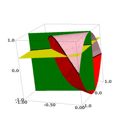
Figure 2: a complete view of the third Weil domain $\overline{\mathcal{W}}_{3}$ (upper left) and three partial views of $\overline{\mathcal{W}}_{3}\cap\mathcal{L}_{3}^{g}$ (for $-1\leq x_{1}\leq 0$): one for $g<g_{3}$ (upper right), one for $g=g_{3}$ (bottom left) and one for $g>g_{3}$ (bottom right). The red (resp. pink) surface is the locus $\{G_{3}^{-}=0\}$ (resp. $\{G_{3}^{+}=0\}$) above $\overline{\mathcal{W}}_{2}$. The dark green almost vertical plane is $x_{2}=\alpha x_{1}+\frac{q-1}{2g}$, the light green almost horizontal plane is $x_{3}=\alpha^{2}x_{1}+\frac{q^{2}-1}{2g\sqrt{q}}$. Their intersection is the black third Ihara line $\mathcal{L}_{3}^{g}$ in genus $g$, which cuts the red surface only for $g\geq g_{3}$.

Theorem 18.

Let $X$ be a smooth projective absolutely irreducible curve over $\mathbb{F}_{q}$ of genus $g$ such that $g>g_{3}=\frac{\sqrt{q}(q-1)}{\sqrt{2}}$. Then, we have

$$\sharp X(\mathbb{F}_{q})-q-1\leq\Biggl{(}\sqrt{a(q)+\frac{b(q)}{g}+\frac{c(q)}{g^{2}}}-1+\frac{1}{q}+\frac{d(q)}{g}\Biggl{)}g\sqrt{q},$$

where

$$\left\{\begin{matrix}a(q)&=&5+\frac{8}{\sqrt{q}}-\frac{1}{q^{2}}\\ b(q)&=&\frac{q-1}{q\sqrt{q}}\Bigl{(}q^{2}-4q\sqrt{q}+2q+4\sqrt{q}-1\Bigr{)}\\ c(q)&=&\frac{q-1}{4q}\Bigl{(}q^{3}-5q^{2}-8q\sqrt{q}-5q-8\sqrt{q}+1\Bigr{)}\\ d(q)&=&\frac{2\sqrt{q}(q-1)^{2}}{q}.\end{matrix}\right.$$

Proof — Let $g>g_{3}$. Referring to the last item in the discussion above the statement of the Theorem, we begin to prove that the unique $-1<\mu_{3}<0$, such that $A_{3}^{g}=P_{3}(\mu_{3})\in\overline{\mathcal{W}}_{3}\cap\mathcal{L}_{3}^{g}\cap\{G_{3}^{-}=0\}$, satisfies criteria 17. Then, we compute the exact value of $\mu_{3}$, which is, by criteria 17 together with Proposition 16, a lower bound for $x_{1}$’s coming from curve over $\mathbb{F}_{q}$. We deduce the Theorem using (3).

Let us prove that $P_{0}=P_{3}(\mu_{3}))$ satisfies the requirements of criteria 17. The first requirement holds true: $A_{3}^{g}\in\{G_{3}^{-}=0\}$. We prove later in corollary 21 that the third one also holds true for any $n\geq 1$. we have only to check the second requirement, that $\partial_{i}G_{3}^{-}(P_{3}^{g}(\mu_{3}))\geq 0$ for $i=2,3$. Since by (10) we have

$$G_{3}^{-}(x_{1},x_{2},x_{3})=\begin{vmatrix}1+x_{3}&x_{1}+x_{2}\\ x_{1}+x_{2}&1+x_{1}\end{vmatrix},$$

we deduce that for any $(x_{1},x_{2},x_{3})\in\mathbb{R}^{3}$,

$$\left\{\begin{matrix}\partial_{2}G_{3}^{-}(P_{3}(x_{1}))&=-2(x_{1}+x_{2})\\ \partial_{3}G_{3}^{-}(P_{3}(x_{1}))&=1+x_{3}.\end{matrix}\right.$$

If $x_{1}=\mu_{3}$, then $P_{0}=A_{3}^{g}=P_{3}(\mu_{3})\in\overline{\mathcal{W}}_{3}\subset]-1,+1[^{3}$, hence

$$\partial_{3}G_{3}^{-}(P_{3}(\mu_{3}))=1+x_{3}(P_{0})>0,$$

so that it remains to prove that $x_{1}(P_{0})+x_{2}(P_{0})\leq 0$.

Since $P_{3}(\mu_{3})=A_{3}^{g}\in\{G_{3}^{-}=0\}\cap\mathcal{L}_{3}^{g}$, we have

$$\left\{\begin{matrix}(x_{1}+x_{2})^{2}&=&(1+x_{1})(1+x_{3})\\ x_{3}&=&\alpha^{2}x_{1}+\frac{q^{2}-1}{2g\sqrt{q}}.\end{matrix}\right.$$

We deduce that $P_{3}(\mu_{3})$ lies on on the plane parabola

$$x_{1}+x_{2}=\pm\sqrt{(1+x_{1})\left(1+\alpha^{2}x_{1}+\frac{q^{2}-1}{2g\sqrt{q}}\right)},$$

and are reduced to check that $P_{3}(\mu_{3})$ lies on on the lower branch

$$x_{1}+x_{2}=-\sqrt{(1+x_{1})\left(1+\alpha^{2}x_{1}+\frac{q^{2}-1}{2g\sqrt{q}}\right)}.$$

The point is that $(x_{1},x_{2})=(-1,1)$ lies on on both branches of this parabola, and that the tangent line to the parabola at this point is the vertical one. Hence, the upper branch defines a concave subset

$$\left\{(x_{1},x_{2})\mid x_{1}\geq-1,\quad x_{2}\geq 1\quad\hbox{and}\quad x_{1}+x_{2}\leq\sqrt{(1+x_{1})\left(1+\alpha^{2}x_{1}+\frac{q^{2}-1}{2g\sqrt{q}}\right)}\right\}$$

of $\mathbb{R}^{2}$, containing $(-1,1)$ and $(0,\sqrt{1+\frac{q^{2}-1}{2g\sqrt{q}}})$ with $\sqrt{1+\frac{q^{2}-1}{2g\sqrt{q}}}>1$. It follows that for any $-1<x_{1}<0$, a point $(x_{1},x_{2})$ lying on the upper parabolic branch lies also on the locus $x_{2}>1$, which cannot hold for $P_{0}=P_{3}(\mu_{3}))\in\overline{\mathcal{W}}_{3}\subset[-1,-1]^{3}$.

It follows that all requirements of criteria 17 hold true for the point $P_{3}(\mu_{3})$, which lies on the branch $x_{1}+x_{2}=-\sqrt{(1+x_{1})(1+\alpha^{2}x_{1}+\frac{q^{2}-1}{2g\sqrt{q}})}$, so that $\mu_{3}$ is a lower bound on $\overline{\mathcal{W}}_{3}\cap\mathcal{H}_{3}^{g}$ for $g>g_{3}$.

Since $P_{3}(\mu_{3})$ lies on $\mathcal{L}_{3}^{g}$, it lies in particular on $x_{2}=\alpha x_{1}+\frac{q-1}{2g}$, so that $\mu_{3}$ is a solution of the quadratic equation

$$(x_{1}+\alpha x_{1}+\frac{q-1}{2g})^{2}=(1+x_{1})(1+\alpha^{2}x_{1}+\frac{q^{2}-1}{2g\sqrt{q}}),$$

where we recall that $\alpha=\frac{1}{\sqrt{q}}$. Solving this equation proves that the only solution in $[-1,0]$ is

$$\mu_{3}=\frac{\frac{q-1}{q}-\frac{2\sqrt{q}(q-1)^{2}}{gq}-\sqrt{a(q)+\frac{b(q)}{g}+\frac{c(q)}{g^{2}}}}{2},$$

hence the Theorem using (3). $\square$

The formula becomes nicer if we let $g$ going to infinity. We obtain the following third order asymptotic bound for Ihara’s constant $A(q)$ (see [Iha81]).

Corollary 19.

The Ihara constant $A(q)$ is bounded above by:

$$A(q)\leq\Biggl{(}\sqrt{5+\frac{8}{\sqrt{q}}-\frac{1}{q^{2}}}-1+\frac{1}{q}\Biggl{)}\sqrt{q}.$$

Remark – For $q$ large the preceding upper bound is equivalent to $(\sqrt{5}-1)\sqrt{q}\simeq 1,236\sqrt{q}$. This is better than the upper bound of $A(q)$ following from Ihara bound

$$A(q)\leq\frac{\sqrt{8q+1}-1}{2},$$

which is equivalent to $\sqrt{2q}\simeq 1,414\sqrt{q}$ for $q$ large. We prove later in Theorem 22 that we can also recover Dinfeld-Vlăduţ and Tsfasman bounds with this viewpoint.

2.6.2 General features

The idea of the algorithm producing numerical values for higher order Weil bounds for given $g,q$ is the following. It computes numerically in a first step an approximation of the unique $-1\leq x_{1}<0$ for which $P_{n}(x_{1})$ lies on the intersection of $\mathcal{L}_{n}^{g}$ with $G_{n}^{-}=0$, and it checks numerically in a second step that this point satisfies criteria 17. This algorithm is valid thanks to Proposition 20 that such an $x_{1}$ as in the first step do exists, at least for $g$ large enough.

Proposition 20.

There exists a sequence $(g_{n})_{n\geq 2}$ such that  $g>g_{n}$ if, and only if, the intersection of the $n$-th Ihara line $\mathcal{L}_{n}^{g}$ in genus $g$ with the interior of the $n$-the Weil domain $\mathcal{W}_{n}$ is a non-empty $x_{1}$-segment $\left]A_{n}^{g},B_{n}^{g}\right[$, with $A_{n}^{g}$ lies on on the hypersurface of $\overline{\mathcal{W}}_{n-1}\times\mathbb{R}$ having equation $G_{n}^{-}=0$, and with $-1\leq x_{1}<0$.

Proof — We keep notations of Section 2.4 and we begin by studying the infinite line $\mathcal{L}_{n}^{\infty}=\{(x_{1},\alpha x_{1},\ldots,\alpha^{n-1}x_{1}),\,x_{1}\in\mathbb{R}\}$, whose points are the $P_{n}^{\infty}(x_{1})$ for $x_{1}\in\mathbb{R}$. This line $\mathcal{L}_{n}^{\infty}$ and the domain $\mathcal{W}_{n}$ have a non empty intersection since the origin of $\mathbb{R}^{n}$ belongs to $\mathcal{W}_{n}\cap\mathcal{L}_{n}^{\infty}$. Since $\mathcal{W}_{n}$ is convex and open, $\mathcal{W}_{n}\cap\mathcal{L}_{n}^{\infty}$ must be a non empty segment $\left]P_{n}^{\infty}(\mu_{n}^{\infty}),P_{n}^{\infty}(\nu_{n}^{\infty})\right[$ for some $-1\leq\mu_{n}^{\infty}<\nu_{n}^{\infty}\leq 1$. Necessarily $\mu_{n}^{\infty}<0$ and $\overline{\mathcal{W}}_{n}\cap\mathcal{L}_{n}^{\infty}=\left[P_{n}^{\infty}(\mu_{n}^{\infty}),P_{n}^{\infty}(\nu_{n}^{\infty})\right]$.

Next, we prove that the point $P_{n}^{\infty}(\mu_{n}^{\infty})$ lies on the hypersurface of $\mathcal{W}_{n-1}\times\mathbb{R}$ having equation $G_{n}^{-}=0$. To relieve the notations, for $\epsilon=\pm$ or nothing, we put $L_{n}^{\epsilon}(x_{1})=G_{n}^{\epsilon}(x_{1},\alpha x_{1},\ldots,\alpha^{n-1}x_{1})$. Let us prove by induction that the abscissa $\mu_{n}^{\infty}$ satisfy

$$\forall n\geq 1,\qquad L_{n}^{-}(\mu_{n}^{\infty})=0\text{ and }L_{m}(\mu_{n}^{\infty})>0,\;\forall m<n.$$ (21)

For $n=1$ this is true from (8): $\mu_{1}=-1$ is the only root of $L_{1}(x_{1})=1+x_{1}$ and satisfies $L_{0}(-1)>0$ since $L_{0}=1$. Suppose that assertion (21) holds true for some $n\geq 1$. By Lemma 7, one has

$$2\underbrace{L_{n}(\mu_{n}^{\infty})}_{=0}=\underbrace{L_{n-1}^{+}(\mu_{n}^{\infty})}_{>0}L_{n+1}^{-}(\mu_{n}^{\infty})+\underbrace{L_{n-1}^{-}(\mu_{n}^{\infty})}_{>0}L_{n+1}^{+}(\mu_{n}^{\infty}),$$

where the underbrace (in)equalities come from the induction hypotheses. We first establish that $L_{n+1}^{+}(\mu_{n}^{\infty})>0$. To this end, let $m$ be the quotient of $n+2$ by $2$. By Lemma 5, one has $G_{n+1}^{+}=\operatorname{Det}(T_{m}-H_{m})$, where $T_{m}$ is a Toeplitz given by (6), while $H_{m}$ is Hankel given by (7). Specializing to the point $(\mu_{n}^{\infty},\alpha\mu_{n}^{\infty},\ldots,\alpha^{n}\mu_{n}^{\infty})$, the Hankel part becomes a rank one matrix:

$$-H_{m}=\alpha^{\frac{(-1)^{n+1}+1}{2}}\times(-\mu_{n}^{\infty})\times{}^{t}(\alpha^{m-1},\ldots,\alpha,1)\times(\alpha^{m-1},\ldots,\alpha,1).$$

This matrix is clearly symmetric positive semi definite. But, for general $A$ and $B$ positive semi-definite symmetric matrices, one has $\det(A+B)\geq\det(A)$ (easy consequence of [HJ90, Corollary 4.3.3]). We deduce by induction hypothesis that, for some $z\in\mathbb{R}^{2n}$,

$$L_{n+1}^{+}(\mu_{n}^{\infty}) =\operatorname{Det}\left(T_{m}(1,\mu_{n}^{\infty},\ldots,\alpha^{m-2}\mu_{n}^{\infty})+H_{m}(z)\right)$$

$$\geq\operatorname{Det}(T_{m}(1,\mu_{n}^{\infty},\ldots,\alpha^{m-2}\mu_{n}^{\infty}))=G_{m-1}(\mu_{n}^{\infty},\ldots,\alpha^{m-2}\mu_{n}^{\infty})=L_{m-1}(\mu_{n}^{\infty})>0$$

holds true. It then follows by (2.6.2) that $L_{n+1}^{-}(\mu_{n}^{\infty})<0$. Since $L_{n+1}(0)=1$, there exists $\mu\in\left]\mu_{n}^{\infty},0\right[$ such that $L_{n+1}(\mu)=0$. Since the points $P_{n}^{\infty}(x_{1})$ with $x_{1}\in\left]\mu_{n}^{\infty},0\right[$ of the line $\mathcal{L}_{n}^{\infty}$ belong to $\mathcal{W}_{n}$, this is the case for the point $P_{n}^{\infty}(\mu)$. Hence one must have $L_{m}(\mu)>0$ for all $m\leq n$ and $L_{n+1}(\mu)=0$. This proves that point $P_{n+1}^{\infty}(\mu)$ belongs to $\overline{\mathcal{W}}_{n+1}$ and that $\mu=\mu_{n+1}$. This concludes the induction, hence in particular $G_{n}^{-}(P_{n}^{\infty}(\mu_{n}^{\infty}))=L_{n}^{-}(P_{n}^{\infty}(\mu_{n}^{\infty}))=0$ as asserted, with moreover $-1\leq\mu_{n}^{\infty}<0$.

Now for finite genus, formula (13) shows that the union ${\mathcal{P}}_{n}=\cup_{g\in\left]0,+\infty\right]}\mathcal{L}_{n}$ is a closed half linear $2$-dimensional plane with parameters $\left(x_{1}\in\mathbb{R},\frac{1}{g}\in\left[0,+\infty\right[\right)$. Hence the intersection ${\mathcal{P}}_{n}\cap\mathcal{W}_{n}$ is a $2$-dimensional convex subset in the closed half plane ${\mathcal{P}}_{n}$. Moreover, we have just seen above that the cut out with the line having parameter $\frac{1}{g}=0$ meet it on an non-empty segment with an end $A_{n}^{\infty}=P_{n}(\mu_{n}^{\infty})\in\{G_{n}^{-}=0\}$ with $-1\|eq\mu_{n}^{\infty}<0$. Since by Proposition 10 the locus $\{(x_{1},\ldots,x_{n})\in\mathcal{W}_{n-1}\mid G_{n}^{-}(x_{1},\ldots,x_{n})>0\}$ is convex, this segment is non empty and meet $G_{n}^{-}=0$ for at least one point with $x_{1}<0$ for a connected subset of the parameter $0\leq\frac{1}{g}<+\infty$ containing $0$, hence have the form $0\leq\frac{1}{g}<\frac{1}{g_{n}}$ for some $0<g_{n}<+\infty$. for such a $g$, the cut out with $\mathcal{L}_{n}^{g}$ is a segment $[A_{n}^{g},B_{n}^{g}]$, with $A_{n}^{g}\neq B_{n}^{g}$ since $g>g_{n}$, with $A_{n}^{g}\in\{G_{3}^{-}=0\}$ and with $-1\leq x_{1}(A_{n}^{g})<0$. The Proposition is proved. $\square$

It turns out that under the assumption that a point on $\mathcal{L}_{n}^{g}$ lies on the locus $\overline{\mathcal{W}}_{n}\cap\{G_{n}^{-}=0\}$ always satisfy the last requirement of criteria 17:

Corollary 21.

Let $n\in\mathbb{N}$, $g>g_{n}$ and $\mu_{n}\in]-1,0[$ such that $P_{n}^{g}(\mu_{n})$ is the point $A_{n}^{g}$ of Proposition 20. Then $\sum_{i=1}^{n}\partial_{i}G_{n}^{-}(P_{n}^{g}(\mu_{n}))\alpha^{i-1}>0$.

Proof — Denote by $\varphi(x_{1})=G_{n}^{-}(P_{n}^{g}(x_{1}))$ for $x_{1}\in{\mathbb{R}}$. This is a ${\mathcal{C}}^{\infty}$ function of the real variable $x_{1}$.

By assumption, $P_{n}^{g}(\mu_{n})\in\{G_{n}^{-}=0\}\cap\mathcal{L}_{n}^{g}$ and $g>g_{n}$, hence by Proposition 9 and Proposition 20 we have $P_{n}^{g}(\mu_{n})=A_{n}^{g}$ and $]P_{n}^{g}(\mu_{n}),B_{n}^{g}[\subset\mathcal{W}_{n}\subset\{G_{n}^{-}>0\}$, and there exists some $\varepsilon>0$, such that

$$\forall x_{1}\in\mathbb{R},\quad\mu_{n}<x_{1}<\mu_{n}+\varepsilon\Longrightarrow P_{n}^{g}(x_{1})\in\{G_{n}^{-}>0\}.$$ (22)

Hence by item 2 of Proposition 9, we have $P_{n}^{g}(x_{1})\in\{G_{n}^{-}>0\}$ for $\mu_{n}<x_{1}<\mu_{n}+\varepsilon$, so that $\varphi(x_{1})>0$ for such $x_{1}$. Since by assumption $\varphi(\mu_{n})=0$, we deduce that

$$0\leq\frac{\mathrm{d}\varphi}{\mathrm{d}t}(\mu_{n})=\frac{\mathrm{d}G_{n}^{-}(P_{n}^{g}(\mu_{n}))}{\mathrm{d}t}=\sum_{i=1}^{n}\partial_{i}G_{n}^{-}(P_{n}^{g}(\mu_{n}))\alpha^{i-1}=\left\langle\nabla G_{n}^{-}(\mu_{n}),\vec{u}\right\rangle,$$

where $\vec{u}=(1,\alpha,\ldots,\alpha^{n-1})$ is a director vector of $\mathcal{L}_{n}^{g}$. Now, suppose by contradiction that $\frac{\mathrm{d}\varphi}{\mathrm{d}t}(\mu_{n})=0$. Then by (2.6.2) the line $\mathcal{L}_{n}^{g}$ would be perpendicular to $\nabla G_{n}^{-}(\mu_{n}^{\infty})$, hence tangent to $\{G_{n}^{-}=0\}$ at $P_{n}^{g}(\mu_{n})=A_{n}^{g}$ by Proposition 20. But $\{G_{n}^{-}\geq 0\}\cap\overline{\mathcal{W}}_{n-1}$ is convex by Proposition 10, so that $\mathcal{L}_{n}^{g}$ would never meet the interior $\{G_{n}^{-}=0\}$, a contradiction with (22). $\square$

It turns out that proving that this points is also always a minimum of the coordinate function $x_{1}$ seems to be difficult for $N\geq 4$. But this is an easy task numerically using criteria 17: this will be done in our magma routine in Section 2.6.3.

2.6.3 Numerical results for $n\geq 4$

We have implemented a routine in magma and leading to the following results.

In the following tabular we give, for genus $g$ such that $1\leq g\leq 52$, and for $q\in\{2,3\}$, the best generalized Weil bound for the number of points on a curve of genus $g$ over $\mathbb{F}_{q}$. The number in brackets corresponds to the optimal order Weil bound. For instance, if this number is $2$, this means that the bound is the well known Ihara bound and that bounds of other orders are not better.

$$\begin{array}[]{|*{4}{ccc|}}\hline\cr g&q=2&q=3&g&q=2&q=3&g&q=2&q=3&g&q=2&q=3\\ \hline\cr 1&5(3)&7(2)&14&16(6)&26(4)&27&25(8)&42(5)&40&34(9)&57(6)\\ 2&6(3)&9(2)&15&17(7)&28(4)&28&26(8)&43(5)&41&35(9)&58(6)\\ 3&7(4)&10(3)&16&18(7)&29(5)&29&27(8)&44(5)&42&35(9)&59(6)\\ 4&8(4)&12(3)&17&18(7)&30(5)&30&27(8)&46(5)&43&36(9)&60(6)\\ 5&9(5)&14(3)&18&19(7)&31(5)&31&28(8)&47(5)&44&37(9)&61(6)\\ 6&10(5)&15(3)&19&20(7)&32(5)&32&29(8)&48(6)&45&37(9)&62(6)\\ 7&11(5)&17(4)&20&21(7)&34(5)&33&29(8)&49(6)&46&38(9)&63(6)\\ 8&11(5)&18(4)&21&21(7)&35(5)&34&30(8)&50(6)&47&38(9)&65(6)\\ 9&12(6)&19(4)&22&22(7)&36(5)&35&31(8)&51(6)&48&39(9)&66(6)\\ 10&13(6)&21(4)&23&23(7)&37(5)&36&31(8)&52(6)&49&40(9)&67(6)\\ 11&14(6)&22(4)&24&23(8)&38(5)&37&32(8)&54(6)&50&40(9)&68(6)\\ 12&15(6)&24(4)&25&24(8)&40(5)&38&33(9)&55(6)&51&41(9)&69(6)\\ 13&15(6)&25(4)&26&25(8)&41(5)&39&33(9)&56(6)&52&42(9)&70(6)\\ \hline\cr\end{array}$$

Comparing with the results available on the web site http://www.manypoints.org/, we unfortunately observe that we do not beat any record, and that we reach the records exactly in those cases were it is held by Osterlé bounds! . So we are pretty sure that there is a link between Osterle bound and the one in this Section, even if we do not know how to relate the two approaches.

2.7 Drinfeld-Vlăduţ and Tsfasman bounds as a bound of infinite order

In this Section, we recover the Drinfeld-Vlăduţ and Tsfasman bounds for the asymptotic of the number of points on curves over $\mathbb{F}_{q}$, giving a new meaning for the defect $\delta$ defined in [Tsf92]. With our point of view, these bounds can be considered as Weil bounds of infinite order.

We consider a sequence $(X_{n})_{n\geq 1}$ of absolutely irreducible smooth projective curves over $\mathbb{F}_{q}$. Let $(g_{n})_{n\geq 1}$ be the genus sequence and for $r\geq 1$ and let $B_{r}(X_{n})$ be the number of points of degree $r$ on $X_{n}$:

$$B_{r}(X_{n})=\sharp\left\{P\in X_{n}(\overline{\mathbb{F}}_{q})\mid\deg(P)=r\right\}.$$

Following Tsfasman, we assume this sequence to be asymptotically exact: this means that $\lim_{n\to+\infty}g_{n}=+\infty$ and that for any $r\geq 1$, the sequence $\left(\frac{B_{r}(X_{n})}{g_{n}}\right)_{n\geq 1}$ admits a limit. Then, as usual, we put

$$\forall r\geq 1,\qquad\beta_{r}\overset{\text{def}}{=}\lim_{n\to+\infty}\frac{B_{r}(X_{n})}{g_{n}}.$$

In the following Theorem, the notations and the normalizations are the same as in Definitions 2 and 4.

Theorem 22.

Let $(X_{n})_{n\geq 1}$ be a sequence of absolutely irreducible smooth projective curves over $\mathbb{F}_{q}$. If this sequence is asymptotically exact, then its defect $\delta$, defined as $\delta=1-\sum_{r=1}^{\infty}\frac{r\beta_{r}}{\sqrt{q^{r}}-1}$, satisfy

$$\delta=\lim_{m\to+\infty}\lim_{n\to+\infty}\frac{\left\|\gamma_{X_{n}}^{0}+\gamma_{X_{n}}^{1}+\cdots+\gamma_{X_{n}}^{m-1}\right\|_{X_{n}}^{2}}{m}.$$

Proof — Thanks to the Gram matrix following Definition 4, we compute

$$\frac{1}{m}\left\|\sum_{i=0}^{m-1}\gamma_{X_{n}}^{i}\right\|_{X_{n}}^{2} =\frac{1}{m}\begin{pmatrix}1&\cdots&1\end{pmatrix}\times\operatorname{Gram}\left(\gamma_{X_{n}}^{0},\ldots,\gamma_{X_{n}}^{m-1}\right)\times\begin{pmatrix}1\\ \vdots\\ 1\end{pmatrix}$$

$$=\frac{1}{m}\left[m+2\sum_{i=1}^{m-1}(m-i)x_{i}\right]$$

$$=1+\frac{1}{m}\sum_{i=1}^{m-1}(m-i)\frac{(q^{i}+1)-\sharp X_{n}(\mathbb{F}_{q^{i}})}{g_{n}q^{\frac{i}{2}}}$$

$$=1+\frac{1}{g_{n}}\sum_{i=1}^{m-1}(m-i)\left(q^{\frac{i}{2}}+q^{-\frac{i}{2}}\right)-\sum_{i=1}^{m-1}\left(1-\frac{i}{m}\right)\sum_{r\mid i}\frac{r}{q^{\frac{i}{2}}}\times\frac{B_{r}(X_{n})}{g_{n}}.$$

Letting $n$ tends to $+\infty$ leads to

$$\lim_{n\to+\infty}\frac{1}{m}\left\|\sum_{i=0}^{m-1}\gamma_{X_{n}}^{i}\right\|_{X_{n}}^{2}=1-\sum_{rs\leq m-1}\left(1-\frac{rs}{m}\right)\frac{r\beta_{r}}{q^{\frac{rs}{2}}}=1-\sum_{r=1}^{m-1}\left(\sum_{s=1}^{\lfloor\frac{m-1}{r}\rfloor}\left(1-\frac{rs}{m}\right)\frac{1}{q^{\frac{rs}{2}}}\right)r\beta_{r}.$$ (23)

To conclude, for any $r,m\geq 1$,we remark that

$$\frac{1}{q^{\frac{r}{2}}-1}-\sum_{s=1}^{\lfloor\frac{m-1}{r}\rfloor}\left(1-\frac{rs}{m}\right)\frac{1}{q^{\frac{rs}{2}}}=\sum_{s=1}^{+\infty}\frac{1}{q^{\frac{rs}{2}}}-\sum_{s=1}^{\lfloor\frac{m-1}{r}\rfloor}\left(1-\frac{rs}{m}\right)\frac{1}{q^{\frac{rs}{2}}}=\sum_{s=\frac{m-1}{r}}^{+\infty}\frac{1}{q^{\frac{rs}{2}}}+\frac{1}{m}\sum_{s=1}^{\lfloor\frac{m-1}{r}\rfloor}\frac{rs}{q^{\frac{rs}{2}}}.$$

Being the remainder of a converging serie, the first term of the last expression tends to zero when $m\to+\infty$; as for the second term it also tends to zero by Cesaro. Therefore

$$\lim_{m\to+\infty}\sum_{s=1}^{\lfloor\frac{m-1}{r}\rfloor}\left(1-\frac{rs}{m}\right)\frac{1}{q^{\frac{rs}{2}}}=\frac{1}{q^{\frac{r}{2}}-1},$$

and the Theorem follows letting $m$ tends to $+\infty$ in (23). $\square$

Just pointing out that a norm is non-negative, Theorem 22 leads to the well-known bound:

$$\boxed{\sum_{r=1}^{\infty}\frac{r\beta_{r}}{\sqrt{q^{r}}-1}\leq 1.}$$ (Tsfasman)

As is well known, Tsfasman bound is itself a refinement of

$$\boxed{\limsup_{n\to+\infty}\frac{\sharp X_{n}(\mathbb{F}_{q})}{g_{n}}\leq\sqrt{q}-1.}$$ (Drinfeld-Vlăduţ)

3 Relative bounds

From now on, we concentrate on the relative situation. Our starting point is a finite morphism $f:X\to Y$ of degree $d$, where $X$ and $Y$ are absolutely irreducible smooth projective curves defined over $\mathbb{F}_{q}$, whose genus are denoted by $g_{X}$ and $g_{Y}$.

3.1 The relative Neron-Severi subspace

The morphism $f\times f$ from $X\times X$ to $Y\times Y$ induces two morphisms

$$(f\times f)_{*}:\operatorname{NS}(X\times X)_{\mathbb{R}}\longrightarrow\operatorname{NS}(Y\times Y)_{\mathbb{R}}\quad\text{and}\quad(f\times f)^{*}:\operatorname{NS}(Y\times Y)_{\mathbb{R}}\longrightarrow\operatorname{NS}(X\times X)_{\mathbb{R}}$$

satisfying $(f\times f)_{*}\circ(f\times f)^{*}=d^{2}\operatorname{Id}_{Y\times Y}$. We put:

$$\varphi=\frac{1}{d}(f\times f)_{*}\qquad\text{and}\qquad\psi=\frac{1}{d}(f\times f)^{*}.$$ (24)

Each of these morphisms can be restricted to the euclidean spaces $({\mathcal{E}}_{X},\left\langle\cdot,\cdot\right\rangle_{X})$ and $({\mathcal{E}}_{Y},\left\langle\cdot,\cdot\right\rangle_{Y})$ associated to the curves $X$ and $Y$ as in Section 1. Recall that both are the image of the orthogonal projections given by (1):

$$p_{X}:\operatorname{NS}(X\times X)_{\mathbb{R}}\longrightarrow{\mathcal{E}}_{X}\qquad\text{and}\qquad p_{Y}:\operatorname{NS}(Y\times Y)_{\mathbb{R}}\longrightarrow{\mathcal{E}}_{Y}.$$

In fact, we still restrict a little bit more the morphisms $\varphi$ and $\psi$. Let $F_{X}:X\to X$ and $F_{Y}:Y\to Y$ be the $q$-Frobenius on $X$ and $Y$. As usual, for $k\geq 0$, we denote by $\Gamma_{F_{X}}^{k}$ the class in $\operatorname{NS}(X\times X)_{\mathbb{R}}$ of the $k$-th iterated of $F_{X}$. We do the same for $\Gamma_{F_{Y}}^{k}$ inside $\operatorname{NS}(Y\times Y)_{\mathbb{R}}$.

Definition 23.

For $i\geq 0$, we put:

$$\gamma_{X}^{i}=\frac{1}{\sqrt{2q^{i}}}p_{X}\left(\Gamma_{F_{X}}^{i}\right)\in{\mathcal{E}}_{X},\qquad\qquad\gamma_{Y}^{i}=\frac{1}{\sqrt{2q^{i}}}p_{Y}\left(\Gamma_{F_{Y}}^{i}\right)\in{\mathcal{E}}_{Y},$$

and we denote by ${\mathcal{F}}_{X}$ and ${\mathcal{F}}_{Y}$ the two subspaces of ${\mathcal{E}}_{X}$ and ${\mathcal{E}}_{Y}$ defined by

$${\mathcal{F}}_{X}=\operatorname{Vect}\left(\gamma_{X}^{i},\;i\geq 0\right)\subset{\mathcal{E}}_{X},\qquad\qquad{\mathcal{F}}_{Y}=\operatorname{Vect}\left(\gamma_{Y}^{i},\;i\geq 0\right)\subset{\mathcal{E}}_{Y}.$$

Remark – Note that the normalization in this Section differs from the one chosen in Definition 3 by a factor $\frac{1}{\sqrt{g}}$. The nice feature of this new normalization is that with this choice, the pull-back of divisor classes between some subspaces of the Neron Severi spaces is isometric, see the next Proposition 24.

For $i\geq 0$ and $j\geq 1$, one has by Lemma 3, with this new normalization for $\gamma^{i}$,

$$\left\|\gamma_{X}^{i}\right\|_{X}=\sqrt{g_{X}}, \left\langle\gamma_{X}^{i},\gamma_{X}^{i+j}\right\rangle_{X}=\frac{(q^{j}+1)-\sharp X(\mathbb{F}_{q^{j}})}{2\sqrt{q^{j}}},$$ (25)

$$\left\|\gamma_{Y}^{i}\right\|_{Y}=\sqrt{g_{Y}}, \left\langle\gamma_{Y}^{i},\gamma_{Y}^{i+j}\right\rangle_{Y}=\frac{(q^{j}+1)-\sharp Y(\mathbb{F}_{q^{j}})}{2\sqrt{q^{j}}}.$$ (26)

In other words, the vectors $\gamma_{X}^{i}$ for $i\geq 0$ lie on in the euclidean sphere of radius $\sqrt{g_{X}}$ in the finite dimensional euclidean vector space ${\mathcal{E}}_{X}$, and the data of the scalar products is equivalent to the datas of the numbers of rational points of $X$ on the finite extensions of $\mathbb{F}_{q}$.

Proposition 24.

Restricted respectively to ${\mathcal{F}}_{X}$ and ${\mathcal{F}}_{Y}$, the morphisms $\varphi$ and $\psi$ satisfy the followings.

1. One has $\varphi\circ\psi=\operatorname{Id}_{{\mathcal{F}}_{Y}}$, the identity map on ${\mathcal{F}}_{Y}$.

2. For all $i\geq 0$, $\varphi(\gamma_{X}^{i})=\gamma_{Y}^{i}$.

3. For all $\gamma\in{\mathcal{F}}_{X}$ and all $\delta\in{\mathcal{F}}_{Y}$, $\left\langle\gamma,\psi\left(\delta\right)\right\rangle_{X}=\left\langle\varphi(\gamma),\delta\right\rangle_{Y}$ .

4. For all $i,j\geq 0$, $\left\langle\psi(\gamma_{Y}^{i}),\psi(\gamma_{Y}^{j})\right\rangle_{X}=\left\langle\gamma_{Y}^{i},\gamma_{Y}^{j}\right\rangle_{Y}$ .

5. The morphism $\psi$ is an isometric embedding $\left({\mathcal{F}}_{Y},\left\langle\cdot,\cdot\right\rangle_{Y}\right)\hookrightarrow\left({\mathcal{F}}_{X},\left\langle\cdot,\cdot\right\rangle_{X}\right)$ and $\psi\circ\varphi$ is the orthogonal projection of ${\mathcal{F}}_{X}$ on its subspace $\psi({\mathcal{F}}_{Y})$.

Proof — Item (1) follows from the identity $(f\times f)_{*}\circ(f\times f)^{*}=d^{2}\operatorname{Id}_{Y\times Y}$. Item (2) follows from the identity $(f\times f)_{*}\Gamma_{F_{X}^{i}}=d\Gamma_{F_{Y}^{i}}$. Item (3) follows from the projection formula for the proper morphism $f\times f:X\times X\rightarrow Y\times Y$. Item (4) follows then from items (1) and (3). Finally, item (5) follow from the preceding ones together with the following Lemma. $\square$

Lemma 25.

Let $\left(E,\left\langle.,.\right\rangle_{E}\right)$ and $\left(F,\left\langle.,.\right\rangle_{F}\right)$ be two finite dimensional euclidean vector spaces. Suppose that $E$ is generated by a family $\{u_{i},i\geq 0\}$ and $F$ is generated by a family $\{v_{j},j\geq 0\}$. Let $\varphi:E\rightarrow F$ and $\psi:F\rightarrow E$ be linear maps satisfying $\varphi\circ\psi=\operatorname{Id}_{F}$ and such that

$$\left\langle\psi(v_{i}),\psi(v_{j})\right\rangle_{E}=\left\langle v_{i},v_{j}\right\rangle_{F}, \forall i,j\geq 0,$$ (27)

$$\left\langle v,\varphi(u)\right\rangle_{F}=\left\langle\psi(v),u\right\rangle_{E}, \forall u\in E,\forall v\in F.$$ (28)

Then, $\psi$ is an isometric embedding from $F$ to $E$ and $\psi\circ\varphi$ is the orthogonal projection from $E$ to $\psi(F)$.

Proof — By (27), the morphism $\psi$ must be an isometric embedding. Let us prove that $\psi\circ\varphi$ is the orthogonal projection on $\psi(F)$. Since $\varphi\circ\psi=\operatorname{Id}_{F}$, we have $(\psi\circ\varphi)^{2}=\psi\circ\varphi\circ\psi\circ\varphi=\psi\circ\varphi$; therefore $\psi\circ\varphi$ is a projector. For $v\in F$, one has $\psi\circ\varphi(\psi(v))=\psi(v)$, again by $\varphi\circ\psi=\operatorname{Id}_{F}$; in other terms $\psi(F)$ is stabilized by $\psi\circ\varphi$. Last, for $u\in E$, one has $u-\psi\circ\varphi(u)\in\psi(F)^{\perp}$. Indeed, for $v\in F$, one has:

$$\left\langle u-\psi\circ\varphi(u),\psi(v)\right\rangle_{E} =\left\langle u,\psi(v)\right\rangle_{E}-\left\langle\psi\circ\varphi(u),\psi(v)\right\rangle_{E}$$

$$=\left\langle\varphi(u),v\right\rangle_{F}-\left\langle\varphi(u),v\right\rangle_{F}$$ by (28)

$$=0.$$

This concludes the proof. $\square$

Definition 26.

Let ${\mathcal{F}}_{X/Y}$ be the subspace $\psi({\mathcal{F}}_{Y})$, called the relative subspace for the morphism $X\rightarrow Y$.

Then we have just proved that

$$\begin{array}[]{ccccc}{\mathcal{F}}_{X}&=&{\mathcal{F}}_{X/Y}&\oplus&{\mathcal{F}}_{X/Y}^{\perp}\\ \leavevmode\hbox to9.78pt{\vbox to2.67pt{\text{[drawing]}}}&&\leavevmode\hbox to9.78pt{\vbox to2.67pt{\text{[drawing]}}}&&\leavevmode\hbox to9.78pt{\vbox to2.67pt{\text{[drawing]}}}\\ u&=&\psi\circ\varphi(u)&+&\left(u-\psi\circ\varphi(u)\right)\end{array} \in \in \in \in \in \in$$

Remark – The absolute case of Section 2 enters in this relative case by choosing any non-constant rational function $X\rightarrow{\mathbb{P}}^{1}$; in this case, the relative space ${\mathcal{F}}_{X/{\mathbb{P}}^{1}}$ is the sub-space of ${\mathcal{E}}_{X}$ generated by the projections of the classes of iterations of the Frobenius morphism.

We are now able to easily compute some norms and scalar products.

Lemma 27.

For any $i\geq 0$, the following decomposition holds true:

$$\gamma_{X}^{i}=\underbrace{\psi(\gamma_{Y}^{i})}_{\in{\mathcal{F}}_{X/Y}}+\underbrace{\left(\gamma_{X}^{i}-\psi(\gamma_{Y}^{i})\right)}_{\in{\mathcal{F}}_{X/Y}^{\perp}}\in{\mathcal{F}}_{X}$$

and one has:

$$\forall i,j\geq 0, \psi(\gamma_{Y}^{i})\perp\gamma_{X}^{j}-\psi(\gamma_{Y}^{j})$$ (29)

$$\forall i\geq 0, \left\|\gamma_{X}^{i}-\psi(\gamma_{Y}^{i})\right\|_{X}=\sqrt{g_{X}-g_{Y}}$$ (30)

$$\forall i\geq 0,\forall j\geq 1, \left\langle\gamma_{X}^{i}-\psi(\gamma_{Y}^{i}),\gamma_{X}^{i+j}-\psi(\gamma_{Y}^{i+j})\right\rangle_{X}=\frac{\sharp Y(\mathbb{F}_{q^{j}})-\sharp X(\mathbb{F}_{q^{j}})}{2\sqrt{q^{j}}}.$$ (31)

Proof — The first norm calculation is just a consequence of Pythagore Theorem:

$$\left\|\gamma_{X}^{i}\right\|_{X}^{2} =\left\|\psi(\gamma_{Y}^{i})\right\|_{X}^{2}+\left\|\gamma_{X}^{i}-\psi\left(\gamma_{Y}^{i}\right)\right\|_{X}^{2}$$ by Pythagore

$$=\left\|\gamma_{Y}^{i}\right\|_{Y}^{2}+\left\|\gamma_{X}^{i}-\psi\left(\gamma_{Y}^{i}\right)\right\|_{X}^{2} \psi$$ since isometric

and thus by (25) and (26)

$$g_{X}=g_{Y}+\left\|\gamma_{X}^{i}-\psi\left(\gamma_{Y}^{i}\right)\right\|_{X}^{2}.$$

Taking intby o account orthogonality, we also easily compute the scalar product:

$$\left\langle\gamma_{X}^{i}-\psi(\gamma_{Y}^{i}),\gamma_{X}^{i+j}-\psi(\gamma_{Y}^{i+j})\right\rangle_{X} =\left\langle\gamma_{X}^{i},\gamma_{X}^{i+j}\right\rangle_{X}-\left\langle\psi\left(\gamma_{Y}^{i}\right),\psi\left(\gamma_{Y}^{i+j}\right)\right\rangle_{X}$$ by orthogonality

$$=\left\langle\gamma_{X}^{i},\gamma_{X}^{i+j}\right\rangle_{X}-\left\langle\gamma_{Y}^{i},\gamma_{Y}^{i+j}\right\rangle_{Y} \psi$$ since isometric

$$=\frac{(q^{j}+1)-\sharp X(\mathbb{F}_{q^{j}})}{2\sqrt{q^{j}}}-\frac{(q^{j}+1)-\sharp Y(\mathbb{F}_{q^{j}})}{2\sqrt{q^{j}}} \text{by~{}(\ref{norme_gamma_X}) and~{}(\ref{norme_gamma_Y})}.$$

The result follows. $\square$

3.2 Number of points in coverings

As applications of this Proposition, we prove in the very same spirit than in Section 2 the following three results. The first one is well known, the others are new. It worth to notice that the first one can be proved using Tate modules of the jacobians of the involved curves (see e.g. [AP95]), whereas up to our knowledge, the others cannot.

Proposition 28.

Suppose that there exists a finite morphism $X\rightarrow Y$. Then we have

$$|\sharp X(\mathbb{F}_{q})-\sharp Y(\mathbb{F}_{q})|\leq 2(g_{X}-g_{Y})\sqrt{q}.$$

Proof — We apply Cauchy-Schwartz inequality to the vectors $\gamma_{X}^{0}-\psi(\gamma_{Y}^{0})$ and $\gamma_{X}^{1}-\psi(\gamma_{Y}^{1})$. Thanks to Lemma 27 specialized to $j=1$ and $i=0,1$, we obtain

$$\left|\frac{\sharp X(\mathbb{F}_{q})-\sharp Y(\mathbb{F}_{q})}{2\sqrt{q}}\right|^{2} =\left|\left\langle\gamma_{X}^{0}-\psi(\gamma_{Y}^{0}),\gamma_{X}^{1}-\psi(\gamma_{Y}^{1})\right\rangle_{X}\right|^{2}$$

$$\leq\|\gamma_{X}^{0}-\psi(\gamma_{Y}^{0})\|_{X}^{2}\times\|\gamma_{X}^{1}-\psi(\gamma_{Y}^{1})\|_{X}^{2}$$

$$=(g_{X}-g_{Y})^{2},$$

hence the Proposition. $\square$

The following Proposition is the relative form of Proposition 14. Of course, although less nice, such upper bounds can be given for any $n$.

Proposition 29.

For any finite morphism $X\rightarrow Y$ with $g_{X}\neq g_{Y}$, we have

$$\sharp X({\mathbb{F}}_{q^{2}})-\sharp Y({\mathbb{F}}_{q^{2}})\leq 2(g_{X}-g_{Y})q-\frac{\Bigl{(}\sharp X({\mathbb{F}}_{q})-\sharp Y({\mathbb{F}}_{q})\Bigr{)}^{2}}{g_{X}-g_{Y}}.$$

Proof — After computating the $3\times 3$ Gram determinant

$$G_{3}(X/Y)=\operatorname{Gram}(\gamma_{X}^{0}-\psi(\gamma_{Y}^{0}),\gamma_{X}^{1}-\psi(\gamma_{Y}^{1}),\gamma_{X}^{2}-\psi(\gamma_{Y}^{2}))$$

using Lemma 27, it is readily seen, with the very same proof, that factorization in Lemma 5 holds also in this relative case, so that there exists two (explicitly given as determinants) factors $G_{n}^{+}(X/Y)$ and $G_{n}^{-}(X/Y)$ ($n=2$ is sufficient here) as in Definition 6, such that $G_{n}(X/Y)=G_{n}^{+}(X/Y)\times G_{n}^{-}(X/Y)$ also holds. Moreover, Proposition 9 also continue to hold, hence for $n=2$, the result follows from $G_{2}^{-}(X/Y)\geq 0$. $\square$

3.3 Number of points in a fiber product

Let

(32)

be a commutative diagram of finite covers of absolutely irreducible smooth projective curves defined over $\mathbb{F}_{q}$. Applying the results of the beginning of this Section to the four morphisms involved in this diagram leads to another diagram between Euclidean spaces

Let us introduce the following hypothesis:

The fiber product $$Y_{1}\times_{Z}Y_{2}$$ is abolutely irreducible and smooth.

Proposition 30.

Suppose that $(H)$ holds, and that $X=Y_{1}\times_{Z}Y_{2}$ in diagram (32). Then

$$\varphi_{X/Y_{2}}\circ\psi_{X/Y_{1}}=\psi_{Y_{2}/Z}\circ\varphi_{Y_{1}/Z}\\$$

on ${\mathcal{F}}_{Y_{1}}$.

Proof — The proof of formula (30) is mainly set theoretic. We write:

$$(p_{2}\times p_{2})_{*}\circ(p_{1}\times p_{1})^{*}\left(\Gamma_{F_{Y_{1}}}\right) =(p_{2}\times p_{2})_{*}\left(\{[(y_{1},y_{2}),(y^{\prime}_{1},y^{\prime}_{2})]\in(Y_{1}\times_{Z}Y_{2})^{2};y^{\prime}_{1}=F_{Y_{1}}(y_{1})\}\right)$$

$$=\{(y_{2},y^{\prime}_{2})\in Y_{2}\times Y_{2};\exists y_{1}\in Y_{1};f_{1}(y_{1})=f_{2}(y_{2});f_{2}(y^{\prime}_{2})=F_{Y_{2}}(f_{1}(y_{1}))\}$$

$$=\deg f_{1}\times\{(y_{2},y^{\prime}_{2})\in Y_{2}\times Y_{2};f_{2}(y^{\prime}_{2})=F_{Y_{2}}(f_{2}(y_{2}))\}$$

$$=\deg f_{1}\times(f_{2}\times f_{2})^{*}(\Gamma_{F_{Z}}).$$

Now, since $Y_{1}\times_{X}Y_{2}$ is assumed to be absolutely irreducible, we have $\deg f_{1}=\deg p_{2}$ and $\deg f_{2}=\deg p_{1}$ in a fiber product setting. Taking into account the normalization (24), and projecting onto ${\mathcal{E}}_{Y_{2}}$ as in Section 4, allow us to conclude. $\square$

This allow us us to compute some other norms and scalar products.

Lemma 31.

Suppose that $(H)$ holds, and that $X=Y_{1}\times_{Z}Y_{2}$ in diagram (32). Then we have in ${\mathcal{F}}_{X}$

$$\psi_{X/Y_{1}}(\gamma_{Y_{1}}^{i}),\psi_{X/Y_{2}}(\gamma_{Y_{2}}^{i}),\psi_{X/Z}(\gamma_{Z}^{i})\\ \in\operatorname{Vect}\left(\psi_{X/Y_{1}}\left(\gamma_{Y_{1}}^{i}-\psi_{Y_{1}/Z}(\gamma_{Z}^{i})\right),\psi_{X/Y_{2}}\left(\gamma_{Y_{2}^{i}}-\psi_{Y_{2}/Z}(\gamma_{Z}^{i})\right),\gamma_{X}^{i}-\psi_{X/Z}(\gamma_{Z}^{i})\right)^{\perp}$$

and

$$\forall i,j\in\mathbb{N}, \psi_{X/Y_{1}}\left(\gamma_{Y_{1}}^{i}-\psi_{Y_{1}/Z}(\gamma_{Z}^{i})\right)\perp\psi_{X/Y_{2}}\left(\gamma_{Y_{2}}^{j}-\psi_{Y_{2}/Z}(\gamma_{Z}^{j})\right).$$

Proof — First, we compute scalar products with $\psi_{X/Y_{1}}(\gamma_{Y_{1}}^{i})$. We have

$$\left\langle\psi_{X/Y_{1}}(\gamma_{Y_{1}}^{i}),\psi_{X/Y_{1}}\left(\gamma_{Y_{1}}^{i}-\psi_{Y_{1}/Z}(\gamma_{Z}^{i})\right)\right\rangle_{X} =\left\langle\gamma_{Y_{1}}^{i},\gamma_{Y_{1}}^{i}-\psi_{Y_{1}/Z}(\gamma_{Z}^{i})\right\rangle_{Y_{1}} \psi_{X/Y_{1}}$$ since is isometric

$$=0,$$ by Lemma 27

$$\left\langle\psi_{X/Y_{1}}(\gamma_{Y_{1}}^{i}),\psi_{X/Y_{2}}\left(\gamma_{Y_{2}^{i}}-\psi_{Y_{2}/Z}(\gamma_{Z}^{i})\right)\right\rangle_{X} =\left\langle\varphi_{X/Y_{2}}\circ\psi_{X/Y_{1}}(\gamma_{Y_{1}}^{i}),\gamma_{Y_{2}^{i}}-\psi_{Y_{2}/Z}(\gamma_{Z}^{i})\right\rangle_{Y_{2}}$$ by prop. 24

$$=\left\langle\psi_{Y_{2}/Z}\circ\varphi_{Y_{1}/Z}(\gamma_{Y_{1}}^{i}),\gamma_{Y_{2}^{i}}-\psi_{Y_{2}/Z}(\gamma_{Z}^{i})\right\rangle_{Y_{2}}$$ by prop. 30

$$=\left\langle\psi_{Y_{2}/Z}(\gamma_{Z}^{i}),\gamma_{Y_{2}^{i}}-\psi_{Y_{2}/Z}(\gamma_{Z}^{i})\right\rangle_{Y_{2}}$$ by prop. 24

$$=0,$$ by Lemma 27

and

$$\left\langle\psi_{X/Y_{1}}(\gamma_{Y_{1}}^{i}),\gamma_{X}^{i}-\psi_{X/Z}(\gamma_{Z}^{i})\right\rangle_{X} =\left\langle\psi_{X/Y_{1}}(\gamma_{Y_{1}}^{i}),\gamma_{X}^{i}-\psi_{X/Y_{1}}(\gamma_{Y_{1}}^{i})+\psi_{X/Y_{1}}\left(\gamma_{Y_{1}}^{i}-\psi_{Y_{1}/Z}(\gamma_{Z}^{i})\right)\right\rangle_{X}$$

$$=0.$$

The same holds for $\psi_{X/Y_{2}}(\gamma_{Y_{2}}^{i})$.

Secondly, we compute scalar products with $\psi_{X/Z}(\gamma_{Z}^{i})=\psi_{X/Y_{\epsilon}}\circ\psi_{Y_{\epsilon}/Z}(\gamma_{Z}^{i})$, for $\epsilon=1,2$. We have:

$$\left\langle\psi_{X/Z}(\gamma_{Z}^{i}),\psi_{X/Y_{\epsilon}}\left(\gamma_{Y_{\epsilon}}^{i}-\psi_{Y_{\epsilon}/Z}(\gamma_{Z}^{i})\right)\right\rangle_{X} =\left\langle\psi_{X/Y_{\epsilon}}\circ\psi_{Y_{\epsilon}/Z}(\gamma_{Z}^{i}),\psi_{X/Y_{\epsilon}}\left(\gamma_{Y_{\epsilon}}^{i}-\psi_{Y_{\epsilon}/Z}(\gamma_{Z}^{i})\right)\right\rangle_{X}$$

$$=\left\langle\psi_{Y_{\epsilon}/Z}(\gamma_{Z}^{i}),\gamma_{Y_{\epsilon}}^{i}-\psi_{Y_{\epsilon}/Z}(\gamma_{Z}^{i})\right\rangle_{Y_{\epsilon}} \psi_{X/Y_{\epsilon}}$$ isometric

$$=0.$$ by Lemma 27

Last, $\left\langle\psi_{X/Z}(\gamma_{Z}^{i}),\gamma_{X}^{i}-\psi_{X/Z}(\gamma_{Z}^{i})\right\rangle_{X}=0$ by Lemma 27. $\square$

In the same way than the use of the orthogonal projections associated to ${\mathcal{F}}_{X/Y}\subset{\mathcal{F}}_{X}$ in the preceding Section, we do the same here with ${\mathcal{F}}_{X/Y_{1}}+{\mathcal{F}}_{X/Y_{2}}\subset{\mathcal{F}}_{X}$.

Lemma 32.

Suppose that $(H)$ holds, and that $X=Y_{1}\times_{Z}Y_{2}$ in diagram (32). For $i\geq 0$, let $\gamma_{12}^{i}$ be the orthogonal projection of $\gamma_{X}^{i}$ onto $\left({\mathcal{F}}_{X/Y_{1}}+{\mathcal{F}}_{X/Y_{2}}\right)^{\perp}$ inside ${\mathcal{F}}_{X}$. Then

$$\gamma_{12}^{i}=\gamma^{i}_{X}-\psi_{X/Y_{1}}(\gamma^{i}_{Y_{1}})-\psi_{X/Y_{2}}(\gamma^{i}_{Y_{2}})+\psi_{X/Z}(\gamma^{i}_{Z}),$$

and one has:

$$\|\gamma_{12}^{i}\|_{X} =\sqrt{g_{X}-g_{Y_{1}}-g_{Y_{2}}+g_{Z}}$$

$$\left\langle\gamma_{12}^{i},\gamma_{12}^{i+j}\right\rangle_{X} =\frac{\sharp Y_{1}(\mathbb{F}_{q^{j}})+\sharp Y_{2}(\mathbb{F}_{q^{j}})-\sharp X(\mathbb{F}_{q^{j}})-\sharp Z(\mathbb{F}_{q^{j}})}{2\sqrt{q^{j}}}.$$

Proof — Clearly $\gamma_{X}^{i}-\gamma_{12}^{i}\in{\mathcal{F}}_{X/Y_{1}}+{\mathcal{F}}_{X/Y_{2}}$. Thanks to orthogonality relations of Lemma 31 and rewriting $\gamma_{12}^{i}$ a little bit like

$$\gamma_{12}^{i}=\left(\gamma^{i}_{X}-\psi_{X/Z}(\gamma_{Z}^{i})\right)-\psi_{X/Y_{1}}\left(\gamma^{i}_{Y_{1}}-\psi_{Y_{1}/Z}(\gamma^{i}_{Z})\right)-\psi_{X/Y_{2}}\left(\gamma^{i}_{Y_{2}})-\psi_{Y_{2}/Z}(\gamma^{i}_{Z})\right),$$

we prove that $\gamma_{12}^{i}\in\left({\mathcal{F}}_{X/Y_{1}}+{\mathcal{F}}_{X/Y_{2}}\right)^{\perp}$.

To compute the norm let us note that in the decomposition

$$\gamma^{i}_{X}-\psi_{X/Z}(\gamma_{Z}^{i})=\left[\psi_{X/Y_{1}}\left(\gamma^{i}_{Y_{1}}-\psi_{Y_{1}/Z}(\gamma^{i}_{Z})\right)+\psi_{X/Y_{2}}\left(\gamma^{i}_{Y_{2}})-\psi_{Y_{2}/Z}(\gamma^{i}_{Z})\right)\right]+\left[\gamma_{12}^{i}\right].$$

The first bracket lies on in ${\mathcal{F}}_{X/Y_{1}}+{\mathcal{F}}_{X/Y_{2}}$, while the second one lies on in $\left({\mathcal{F}}_{X/Y_{1}}+{\mathcal{F}}_{X/Y_{2}}\right)^{\perp}$. Applying Pythagore again, we deduce that

$$\left\|\gamma^{i}_{X}-\psi_{X/Z}(\gamma_{Z}^{i})\right\|_{X}^{2} =\left\|\psi_{X/Y_{1}}\left(\gamma^{i}_{Y_{1}}-\psi_{Y_{1}/Z}(\gamma^{i}_{Z})\right)+\psi_{X/Y_{2}}\left(\gamma^{i}_{Y_{2}}-\psi_{Y_{2}/Z}(\gamma^{i}_{Z})\right)\right\|_{X}^{2}+\left\|\gamma_{12}^{i}\right\|_{X}^{2}$$

$$=\left\|\psi_{X/Y_{1}}\left(\gamma^{i}_{Y_{1}}-\psi_{Y_{1}/Z}(\gamma^{i}_{Z})\right)\right\|_{X}^{2}+\left\|\psi_{X/Y_{2}}\left(\gamma^{i}_{Y_{2}})-\psi_{Y_{2}/Z}(\gamma^{i}_{Z})\right)\right\|_{X}^{2}+\left\|\gamma_{12}^{i}\right\|_{X}^{2}$$

$$=\left\|\gamma^{i}_{Y_{1}}-\psi_{Y_{1}/Z}(\gamma^{i}_{Z})\right\|_{Y_{1}}^{2}+\left\|\gamma^{i}_{Y_{2}}-\psi_{Y_{2}/Z}(\gamma^{i}_{Z})\right\|_{Y_{2}}^{2}+\left\|\gamma_{12}^{i}\right\|_{X}^{2}.$$

Lemma 27 allows us to conclude since

$$\left\|\gamma_{12}^{i}\right\|_{X}^{2} =\left\|\gamma^{i}_{X}-\psi_{X/Z}(\gamma_{Z}^{i})\right\|_{X}^{2}-\left\|\gamma^{i}_{Y_{1}}-\psi_{Y_{1}/Z}(\gamma^{i}_{Z})\right\|_{Y_{1}}^{2}-\left\|\gamma^{i}_{Y_{2}}-\psi_{Y_{2}/Z}(\gamma^{i}_{Z})\right\|_{Y_{2}}^{2}$$

$$=\left(g_{X}-g_{Z}\right)-\left(g_{Y_{1}}-g_{Z}\right)-\left(g_{Y_{2}}-g_{Z}\right).$$

In the same way, the calculation of $\left\langle\gamma_{12}^{i},\gamma_{12}^{i+j}\right\rangle$ is a consequence of the computation of the scalar product $\left\langle\gamma^{i}_{X}-\psi_{X/Z}(\gamma_{Z}^{i}),\gamma^{i+j}_{X}-\psi_{X/Z}(\gamma_{Z}^{i+j})\right\rangle$. $\square$

Last we can prove the following results.

Theorem 33.

Let $X,Y_{1},Y_{2}$ and $Z$ be absolutely irreducible smooth projective curves in a cartesian diagram (32) of finite morphisms. Suppose that the fiber product $Y_{1}\times_{Z}Y_{2}$ is also absolutely irreducible and smooth. Then

$$\left|\sharp X(\mathbb{F}_{q})-\sharp Y_{1}(\mathbb{F}_{q})-\sharp Y_{2}(\mathbb{F}_{q})+\sharp Z(\mathbb{F}_{q})\right|\leq 2(g_{X}-g_{Y_{1}}-g_{Y_{2}}+g_{Z})\sqrt{q}.$$

Proof — First, for $X=Y_{1}\times_{Z}Y_{2}$ the result is a direct consequence of Cauchy-Schwartz inequality applied to $\gamma_{12}^{0}$ and $\gamma_{12}^{1}$ thanks to Lemma 31 since $(H)$ holds by assumption.

Now, for general $X$ satisfying the assumptions of the Theorem, we have by the universal property of the fibered product a finite morphism $X\rightarrow Y_{1}\times_{Z}Y_{2}$. By triangular inequality, and using Proposition 28 together with the result for $X$, we have

$$\left|\sharp X(\mathbb{F}_{q})-\sharp Y_{1}(\mathbb{F}_{q})-\sharp Y_{2}(\mathbb{F}_{q})+\sharp Z(\mathbb{F}_{q})\right| \leq|\sharp X({\mathbb{F}}_{q})-\sharp Y_{1}\times_{Z}Y_{2}({\mathbb{F}}_{q})|$$

$$+\left|\sharp Y_{1}\times_{Z}Y_{2}(\mathbb{F}_{q})-\sharp Y_{1}(\mathbb{F}_{q})-\sharp Y_{2}(\mathbb{F}_{q})+\sharp Z(\mathbb{F}_{q})\right|$$

$$\leq 2(g_{X}-g_{Y_{1}\times_{Z}Y_{2}})\sqrt{q}+2(g_{Y_{1}\times_{Z}Y_{2}}-g_{Y_{1}}-g_{Y_{2}}+g_{Z})\sqrt{q}$$

$$=2(g_{X}-g_{Y_{1}}-g_{Y_{2}}+g_{Z})\sqrt{q}$$

and the Theorem is proved. $\square$

It worth to notice that Theorem 33 cannot holds without any hypothesis. For instance, if $X=Y_{1}=Y_{2}$ and the morphisms $Y_{i}\rightarrow Z$ are equal, then the right hand side equals $2(g_{X}-2g_{X}+g_{Z})\sqrt{q}=-2(g_{X}-g_{Z})\sqrt{q}$, a negative number! In this case, the Theorem doesn’t apply since $Y_{1}\times_{Z}Y_{2}$ is not irreducible.

Remark – For $Y_{1}\times_{Z}Y_{2}$ to be absolutely irreducible, it suffices that the tensor product of function fields $\mathbb{F}_{q}(Y_{1})\otimes_{\mathbb{F}_{q}(Z)}\mathbb{F}_{q}(Y_{2})$ to be an integral domain. For $(Q_{1},Q_{2})\in Y_{1}\times_{Z}Y_{2}$ to be smooth it is necessary and sufficient that at least one of the morphism $Y_{i}\to Z$ is unramified at $Q_{i}$.

4 Questions

In this Section, we suggest a few questions raised by the viewpoint of this article.

1. Numerical calculations using our algorithm make it possible that the genus sequence $(g_{n},n\in\mathbb{N})$ whose existence is asserted in Proposition 20 has, at least asymptotically, a quite nice behaviour. It seems that for fixed $n\geq 1$, there do exists a constant $0<c_{n}<1$, such that for $q$ large,

   $$g_{n}\sim c_{n}\sqrt{q}^{n},$$

   with moreover $\lim_{n\to+\infty}c_{n}=1$. Of course, we have proved that $c_{2}=\frac{1}{2}$ and $c_{3}=\frac{1}{\sqrt{2}}$.

   It numerically also seems that for any $n\geq 1$ and any $q$,

   $$g_{n}<\frac{\sqrt{q}^{n+1}}{\sqrt{q}-1}.$$

2. Is it true that the first requirement of criteria 17 implies the second one, in the same way that it do implies the third one as proved in corollary 21 ? It turns out that numerically, our algorithm shows that this holds true for all pairs $(g,q)$ we have tested. We gave up this question when we became aware that our bounds seems to be equivalent to Oesterlé’s.

3. Why do the upper bounds obtained in this article always coincide numerically with Osterlé’s one ?

4. In view of the hope to write down explicitly Weil bounds of order $n\geq 4$, it is necessary to solve a one variable polynomial equation on $x_{1}$ of degree $\lceil\frac{n+1}{2}\rceil$, which is greater than 5 for $n\geq 8$. This polynomial equation is, eliminating $\frac{1}{g}$, the resultant

   $$\hbox{Res}_{\frac{1}{g}}\left(G_{n}^{-}(P_{n}^{g}(x_{1})),G_{n}^{+}(P_{n}^{g}(x_{1}))\right)\in\mathbb{Q}\left(\frac{1}{{\sqrt{q}}}\right)[x_{1}].$$

   Do this polynomial have solvable Galois group over the rational function field $\mathbb{Q}\left(\frac{1}{{\sqrt{q}}}\right)$ ?

5. Is there a nice interpretation in this framework for the number of rational points of the Jacobian $\hbox{Jac}(X)$ of a curve $X$ ? In the affirmative, same question for the Prym variety associated to an unramified double cover $X\rightarrow Y$ ?

6. Do the viewpoint of this article can be extended to higher dimensional varieties ?

7. As explained in the article, the geometry and the arithmetic of $X$ are traduced via Hodge Index Theorem to an euclidean property throught Gram determinants by $P_{n}(X)\in\overline{\mathcal{W}}_{n}$, and its arithmetic by $P_{n}(X)\in\mathcal{H}_{n}^{g}$ through Ihara’s constraints, so that upper bounds for $\sharp X(\mathbb{F}_{q})$ are derived from the lower bound for $x_{1}$ on $\overline{\mathcal{W}}_{n}\cap\mathcal{H}_{n}^{g}$.

   Any other constraint coming either from the geometry or the arithmetic of $X$ is likely to reduce the domain $\mathcal{W}_{n}\cap\mathcal{H}_{n}^{g}$, making possible that the $x_{1}$ function on the new domain as greater lower bound. For instance, do the records obtained in the table http://www.manypoints.org/, better than Osterlé bound, can be understood in this way ?

References

- [AP95] Yves Aubry and Marc Perret, Coverings of singular curves over finite fields, Manuscripta Math. 88 (1995), no. 4, 467–478. MR 1362932 (97g:14022)
- [Har77] Robin Hartshorne, Algebraic geometry, Graduate Texts in Mathematics, vol. 52, Springer, 1977.
- [HJ90] Roger A. Horn and Charles R. Johnson, Matrix analysis, Cambridge University Press, Cambridge, 1990, Corrected reprint of the 1985 original.
- [HU96] Jean-Baptiste Hiriart-Urruty, L’optimisation, Que sais-je ?, PUF, 1996.
- [Iha81] Yasutaka Ihara, Some remarks on the number of rational points of algebraic curves over finite fields, J. Fac. Sci. Univ. Tokyo Sect. IA Math. 28 (1981), no. 3, 721–724 (1982). MR 656048 (84c:14016)
- [Sha94] Igor R. Shafarevich, Basic algebraic geometry 1, Springer-Verlag, 1994, — N∘ 31.
- [Tsf92] Michael A. Tsfasman, Some remarks on the asymptotic number of points, Coding theory and algebraic geometry (Luminy, 1991), Lecture Notes in Math., vol. 1518, Springer, Berlin, 1992, pp. 178–192. MR 1186424 (93h:11064)
- [Wei48] André Weil, Sur les courbes algébriques et les variétés qui s’en déduisent, Actualités Sci. Ind., no. 1041 = Publ. Inst. Math. Univ. Strasbourg 7 (1945), Hermann et Cie., Paris, 1948.
- [Zar95] Oscar Zariski, Algebraic surfaces, Classics in Mathematics, Springer-Verlag, Berlin, 1995, With appendices by S. S. Abhyankar, J. Lipman and D. Mumford, Preface to the appendices by Mumford, Reprint of the second (1971) edition. MR 1336146 (96c:14024)